Article

A New Approach for the Development of Grid Models Calculating Tropospheric Key Parameters over China

1
College of Geomatics and Geoinformation, Guilin University of Technology, Guilin 541004, China
2
Beidou Navigation Department, Natural Resources Information Center of Guangxi Zhuang Autonomous Region, Nanning 530028, China
*
Author to whom correspondence should be addressed.
Remote Sens. 2021, 13(17), 3546; https://0-doi-org.brum.beds.ac.uk/10.3390/rs13173546
Submission received: 6 August 2021 / Revised: 3 September 2021 / Accepted: 4 September 2021 / Published: 6 September 2021
(This article belongs to the Special Issue BDS/GNSS for Earth Observation)

Abstract

:
Pressure, water vapor pressure, temperature, and weighted mean temperature (Tm) are tropospheric parameters that play an important role in high-precision global navigation satellite system navigation (GNSS). As accurate tropospheric parameters are obligatory in GNSS navigation and GNSS water vapor detection, high-precision modeling of tropospheric parameters has gained widespread attention in recent years. A new approach is introduced to develop an empirical tropospheric delay model named the China Tropospheric (CTrop) model, providing meteorological parameters based on the sliding window algorithm. The radiosonde data in 2017 are treated as reference values to validate the performance of the CTrop model, which is compared to the canonical Global Pressure and Temperature 3 (GPT3) model. The accuracy of the CTrop model in regards to pressure, water vapor pressure, temperature, and weighted mean temperature are 5.51 hPa, 2.60 hPa, 3.09 K, and 3.35 K, respectively, achieving an improvement of 6%, 9%, 10%, and 13%, respectively, when compared to the GPT3 model. Moreover, three different resolutions of the CTrop model based on the sliding window algorithm are also developed to reduce the amount of gridded data provided to the users, as well as to speed up the troposphere delay computation process, for which users can access model parameters of different resolutions for their requirements. With better accuracy of estimating the tropospheric parameters than that of the GPT3 model, the CTrop model is recommended to improve the performance of GNSS positioning and navigation.

1. Introduction

Tropospheric delay is one of the major factors affecting global navigation satellite system (GNSS) positioning. The vertical distribution of tropospheric parameters is strongly affected by Earth’s gravity. It is difficult to accurately monitor and invert the description and modeling of tropospheric parameters under the influence of many factors. In the geodetic analysis of GNSS and Very Long Baseline Interferometry (VLBI) observations, the slant tropospheric delays are generally mapped into the zenith direction (zenith tropospheric delay, ZTD) through mapping functions. The ZTD is separated into two parts, namely, the zenith hydrostatic delay (ZHD) and the zenith wet delay (ZWD). The ZHD is usually calculated by the Saastamoinen model [1] from surface pressure measurements. The ZWD is estimated in the data analysis or approximated by models such as the Saastamoinen model, which uses parameters such as the temperature and water vapor pressure as input. Furthermore, the weighted mean temperature (Tm) is also an essential parameter that is indispensable in obtaining precipitable water vapor (PWV) from the zenith wet delay. Therefore, pressure, water vapor pressure, temperature, and Tm are key parameters that are used as input data to obtain tropospheric delay information. It is of great significance to monitor temperature, pressure, water vapor pressure, Tm, and other tropospheric parameters for high-precision GNSS positioning and navigation, as well as GNSS meteorologic applications [2,3].
In addition, floods and droughts have been caused by extreme weather frequently. Severe weather, such as strong regional convection, and large-scale climate anomalies have brought on heavy economic losses and casualties in recent years [4,5,6]. With increasing requirements for high-precision GNSS positioning, and in-depth research in fields such as climate change and extreme weather generation mechanisms, the demand for real-time and high-spatiotemporal-resolution tropospheric parameters is increasing.
There are two main types of tropospheric parameter models according to the methods used for modeling. The Hopfield model [7], Saastamoinen model, and Black model [8] are the classic tropospheric delay models which are based on in situ meteorological parameters. Since conventional GNSS receivers are unavailable for measurements, the use of the aforementioned classic tropospheric delay models is restricted to a certain extent. As space technologies such as GNSS and VLBI are widely used in the navigation and guidance of various space vehicles as well as for the needs of climate change and weather forecasting, the real-time and high spatial resolution of meteorological parameters are particularly important [9].
Therefore, developing regional or global empirical tropospheric delay models based on atmosphere analysis data has attracted widespread attention [10,11,12,13,14,15,16]. Empirical meteorological models, such as the University of New Brunswick (UNB) models [17,18], the European Geo-stationary Navigation Overlay System (EGNOS) model [19], the TropGrid model [20,21], and the GPT models [22,23,24,25] have been developed, aimed at directly obtaining high-precision tropospheric parameters through the model without measured meteorological parameters. The UNB3 model was stored by tabulated meteorological data, which divides the latitude into five intervals. The EGNOS model was established by simplifying the UNB3 model, and the formula is different from that of the UNB3 model. Only the day of the year (DOY) and the location of the station are needed when applying this model, which is used in GNSS satellite navigation enhancement systems. The authors of [20] developed the TropGrid model considering the diurnal variations of parameters, but neglect the semiannual variations. The GPT model was established based on the ERA-40 reanalysis data. However, the GPT model only considers the annual variations of the parameters. The authors of [23] developed the GPT2 model, which considers the semiannual variations of parameters, by analyzing 10-year ECMWF ERA-Interim data with resolutions of 5° × 5° and 1° × 1°. Considered to be the tropospheric model with the highest precision for quite a long time, two meteorological parameters were added to the GPT2w model based on GPT2. GPT3 is the latest generation model for an upgraded version of GPT2w. Two parameters of gradients in the east and north direction were added to the GPT3 model [26,27].
The aforementioned tropospheric delay models have performed well in GNSS meteorology. In this work, a new approach is introduced to develop an empirical tropospheric delay model providing meteorological parameters based on the second modern-era retrospective analysis for research and applications (MERRA-2) data. The new empirical model could be used to serve real-time GNSS positioning and navigation.

2. Data and Methods

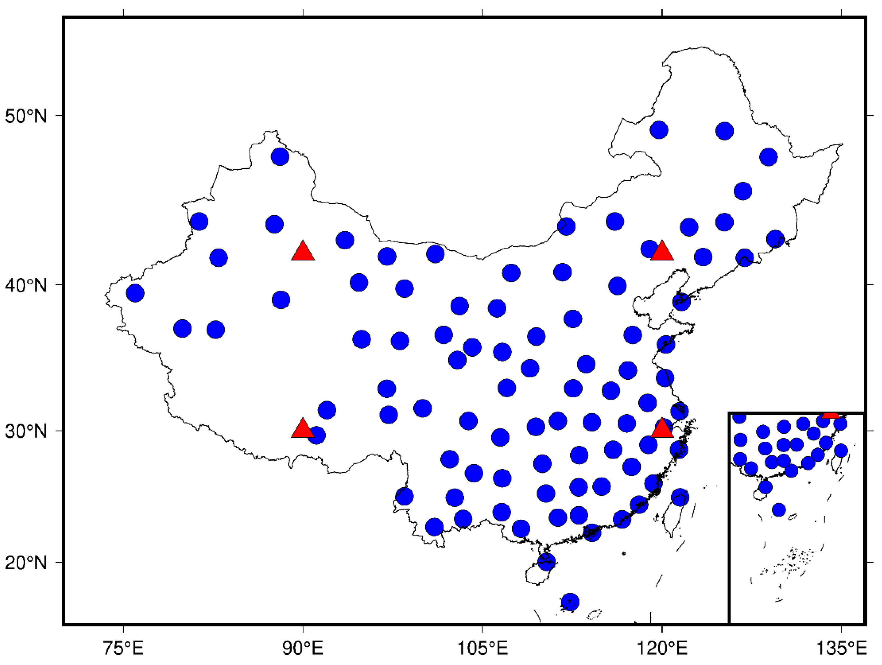
2.1. Radiosonde Data

The radiosonde data provide measured meteorological parameters from the ground to a height of about 30 km at more than 1500 stations around the world. There are 89 radiosonde stations over China as shown in Figure 1. The radiosonde data are obtained based on the actual measurements of meteorological sensors on the sounding balloon, which has high accuracy and credibility. However, radiosonde balloons are extremely susceptible to other disturbance factors, such as weather factors and clouds, during the ascent. Different types of sounding sensors show their own system deviations, as well as equipment failures, which lead to phenomena such as missing data. Although radiosonde data shows some disadvantages, they are still widely used to validate measurement results [27,28].

2.2. MERRA-2 Reanalysis Product Data

MERRA-2 is the latest atmospheric reanalysis product comprising of data beginning in 1980. It is provided by the National Aeronautics and Space Administration (NASA) [29,30] with a spatial resolution of 0.625° × 0.5° (lon. × lat.) and a temporal resolution of 6 h. MERRA-2 replaces the original MERRA reanalysis dataset using an upgraded version of the Goddard Earth Observing System Model, Version 5 (GEOS-5) data assimilation system [31], and the Gridpoint Statistical Interpolation (GSI) analysis scheme [32,33,34]. It is also the first long-term global reanalysis product that assimilates space-based observations of aerosols in the climate system and represents their interactions with physical processes [34]. In addition, MERRA-2 tends to minimize the spurious variations related to inhomogeneity in the observational records and achieves a global balance between evaporation and precipitation through the mass conservation constraint [35]. Temperature, pressure, and specific humidity can be obtained by MERRA-2 data. The water vapor pressure and Tm can be calculated by the following equations:
e = s h · P / 0.622
T m = h e T d h h e T 2 d h
where s h denotes the specific humidity, P is the pressure, h is the height, e is the water vapor pressure, and T is the temperature.

2.3. Analysis of Model Parameters

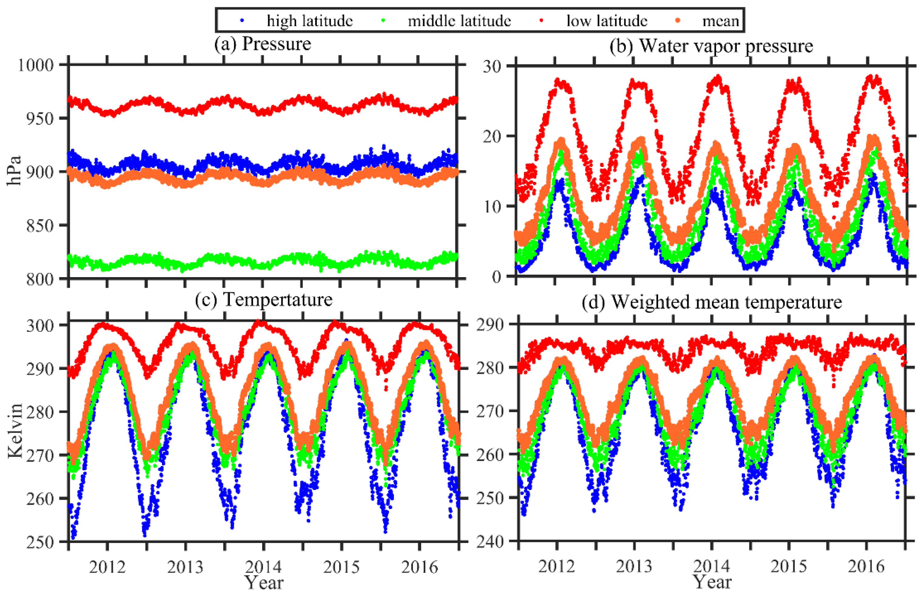
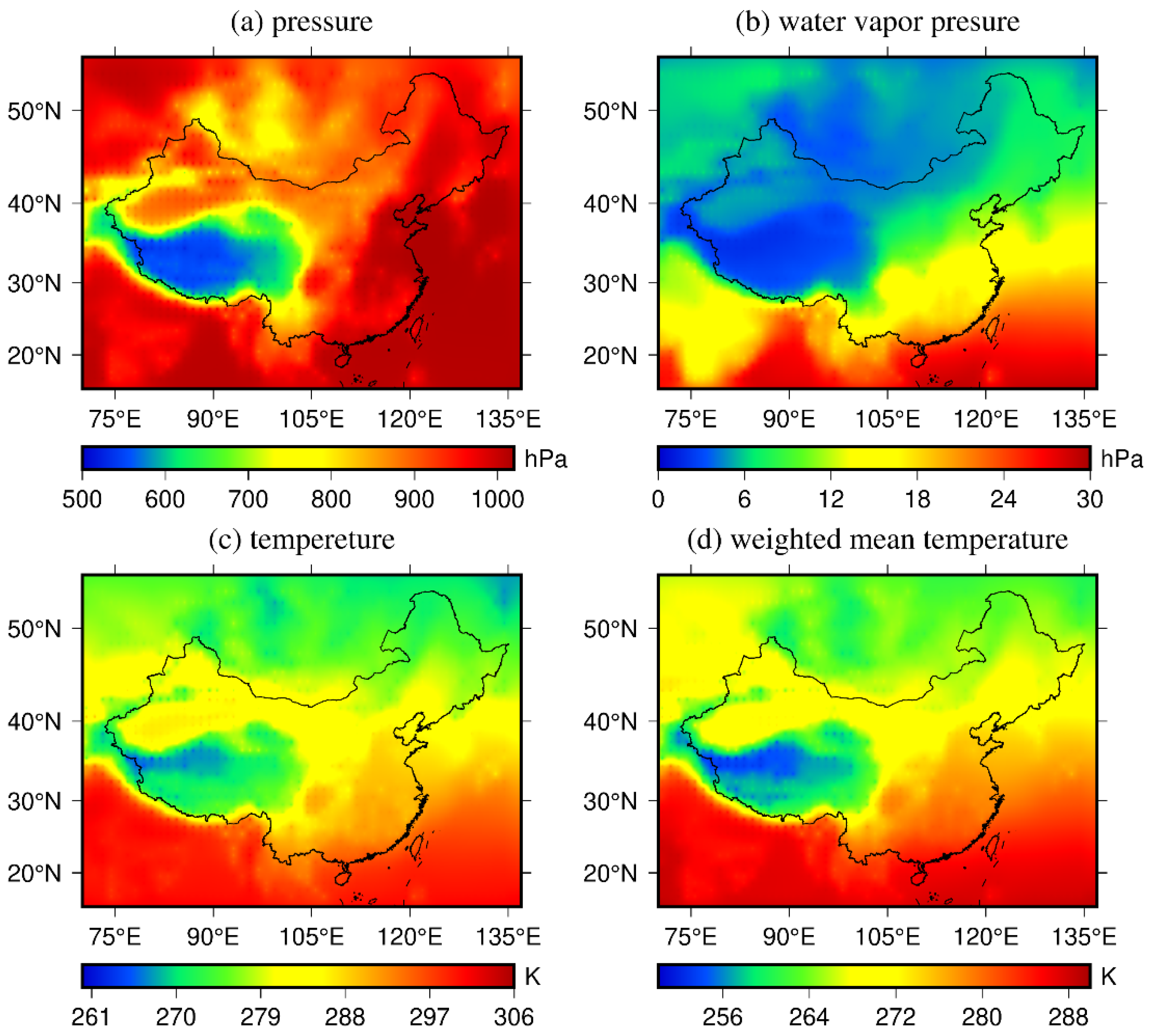
2.3.1. Analysis of Tropospheric Parameters

Analysis of the spatiotemporal characteristics of tropospheric parameters plays an important part in modeling. Some reports have suggested that Tm or temperature are related to height [36,37]. Four representative grid points over China shown in Figure 1 are chosen to determine the daily mean temperature in 2016 for analyzing the correlations between temperature and height. The temperature in each standard pressure level of MERRA-2 is interpolated upon a number of the same heights, and the result is shown in Figure 2. When geopotential height increases, the temperature decreases. There is a correlation between the temperature and the geopotential height of the four grid points over China, which can be expressed as follows:
T = γ · δ h + k
where γ denotes the temperature lapse rate, δ h is the height, and k is a constant.
The Bevis formula [38,39] shows the relationship between the surface temperature and Tm, which can be expressed as Tm = 70.2 + 0.72Ts; thus, the spatial and temporal characteristics of Tm are similar to those of Ts. However, the Bevis formula is only an approximate relationship, and separate models for Tm and temperature are developed in this paper.
Tm, temperature, pressure, and water vapor pressure data provided by the MERRA-2 reanalysis data from 2012 to 2016 are divided into three intervals (15°N–30°N, 30°N–40°N, and 40°N–55°N) according to latitude in order to calculate the time series and to analyze the correlations between the parameters and latitude; the result is shown in Figure 3. All the tropospheric parameters show obvious characteristics of annual and semiannual variations. The peak value of the Tm, temperature, and water vapor pressure in one year appears in the middle of the year, showing symmetrical distribution. In addition, as the latitude increases, the aforementioned values gradually decrease, which indicates the correlation to latitude. The Tm ranges from 245 K to 280 K in the high latitude and middle latitude regions, while it ranges from 280 K to 285 K in the low latitude regions. The temperature ranges from 250 K to 295 K in the high latitude regions and middle latitude areas, while it ranges from 290 K to 300 K in the low latitude regions, which displays more stable temperatures. Pressure shows the largest value in the low latitude regions, while it appears smallest in the middle latitude regions. The water vapor pressure value ranges from 0 hPa to 20 hPa in the high latitude regions and middle latitude areas, while it ranges from 10 hPa to 30 hPa in the low latitude areas, which appears more stable.
MERRA-2 reanalysis data are used to analyze the spatial and temporal characteristics of meteorological parameters. It can be found that these tropospheric parameters are related to latitude and height, and they all have the characteristics of annual and semiannual changes. To further analyze the influence of spatial factors on the tropospheric parameters, the annual mean of the tropospheric parameters at each MERRA-2 grid point over China are determined, and the result is shown in Figure 4. The annual mean values of the tropospheric parameters in the western region are lower than those in other regions over China due to the high altitude in this area. It also has obvious characteristics indicating that the annual average values of the tropospheric parameters in high latitude areas are lower than those in the low- and middle-latitude areas. Furthermore, all the parameters show significant correlations for latitude and longitude.

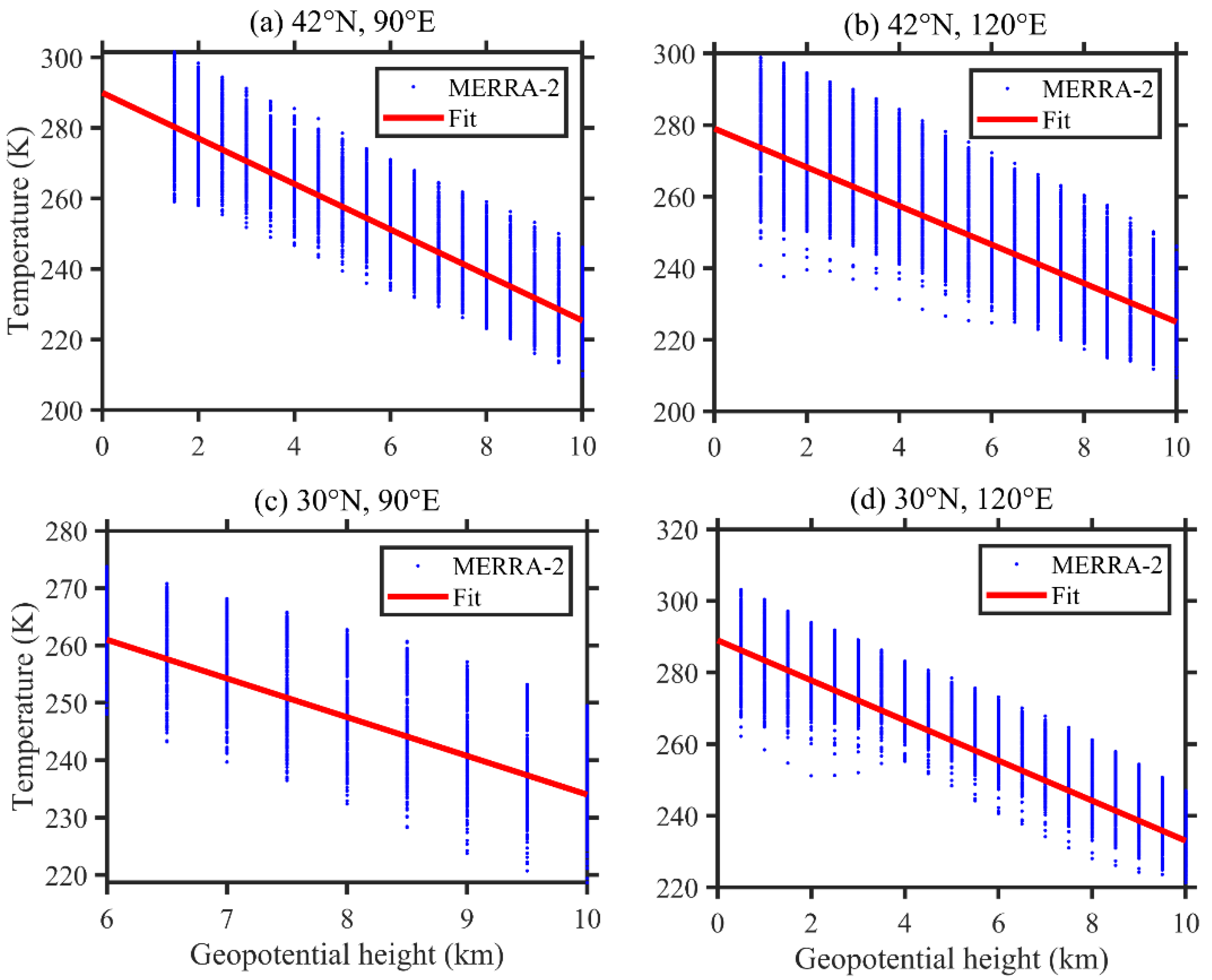
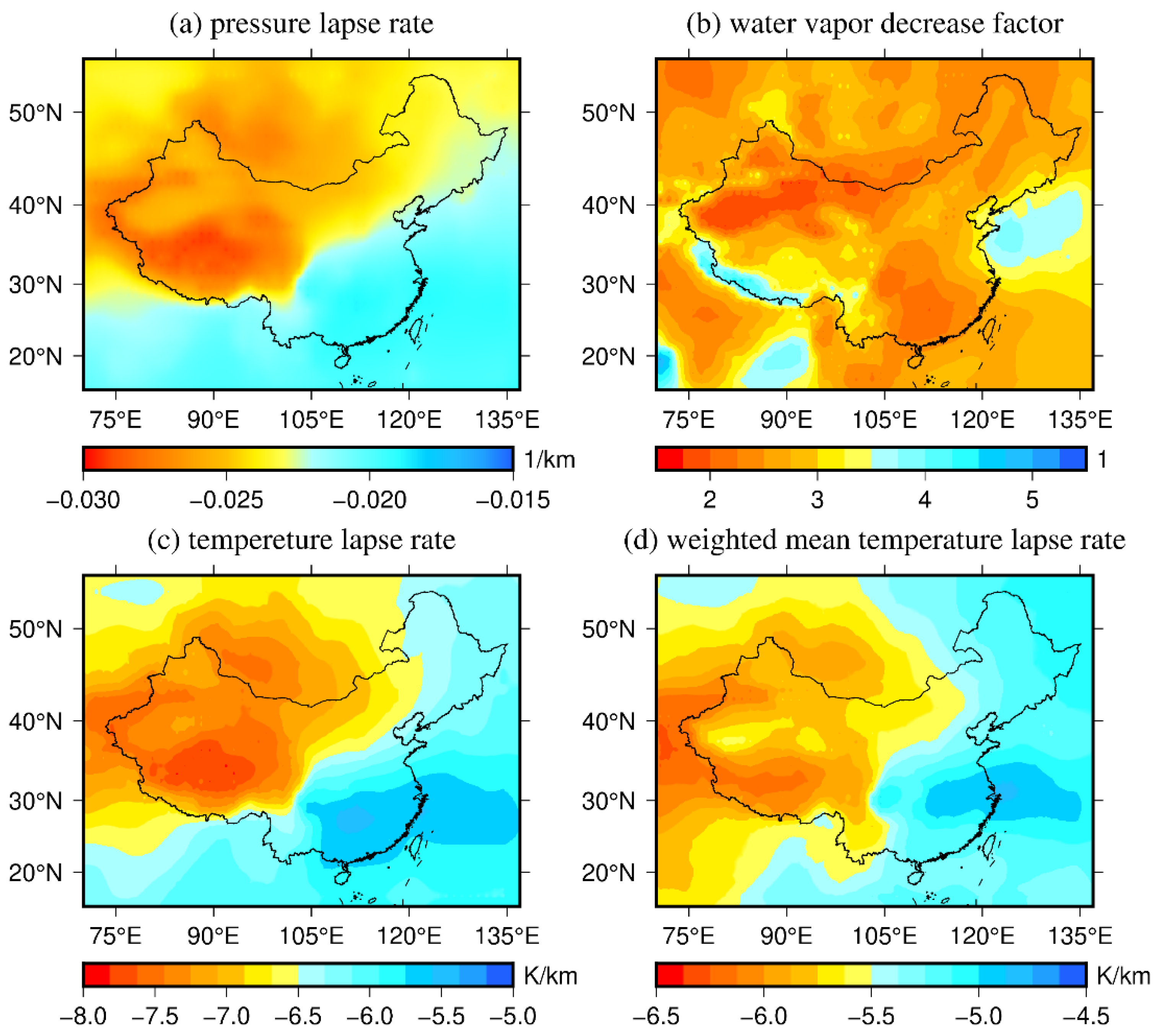
2.3.2. Analysis of the Characteristics of the Lapse Rate

Analysis of the spatiotemporal characteristics of the lapse rate parameters also plays an important part in modeling. When ruling out the differences in elevation data between the different data sources, such as the ellipsoidal height and the geopotential height, the elevation of GNSS and radiosonde stations is inconsistent with the height of the grid point. It must be considered that height correction in the vertical dimension plays an important role in modeling, because these tropospheric parameters are sensitive to height, showing notable changes in the vertical direction. If their vertical changes are properly considered, the model will be able to have better performance at different heights.
The changes in temperature and Tm along the vertical direction are usually adopted to be expressed by the linear function [20,40]. The exponential function is usually adopted to express the changes in pressure [24,25] and water vapor pressure along the vertical direction [21]. In this paper, conventional methods are used to carry out height correction, and they have been adopted in the GPT3 model and other tropospheric delay models. Equations (4)–(7) are for Tm, temperature, pressure, water vapor pressure, and pressure:
T m U = T m G γ · ( H U H G )
T U = T G β · ( H U H G )
e U = e G · ( P U / P G ) λ + 1
P U = P G [ 1 β T G ( H U H G ) ] g · M R · β
where T m U , T U , e U , and P U refer to the meteorological values at the station; T m G , T G , e G , and P G represent the meteorological values at the grid point; H U and H G denote the height at the station and the grid point, respectively; and γ , β , and λ are the lapse rates. M refers to the molar mass of dry air (28.965·10−3 kg/mol), R represents the universal gas constant (8.31432 J/K·mol), and g denotes the gravitational coefficient. A new parameter τ is introduced to show the proportion of temperature and temperature lapse rate, which can be expressed as:
P U = P G [ 1 τ ( H U H G ) ] g · M R · β
λ can be obtained by Equation (6) or (9). In this work, λ is obtained by fitting Equation (9):
Z W D = 10 6 ( k 2 + k 3 / T m ) R d ( λ + 1 ) g e s
where k 2 and k 3 denote the refractive index constants. R d refers to the specific gas constant for the dry constituents [41].
To further analyze the distribution of the annual mean of the lapse rate parameters, the data over China are determined from 2012 to 2016, and the result is shown in Figure 5. The annual mean value of the pressure lapse rate, temperature lapse rate, and Tm lapse rate shows obvious geographical characteristics over China. The values are smaller in the west of China than in other regions, which is due to the higher elevation in the western region. The distribution of the water vapor decrease factor is different from the others, which shows that the values in the northeast and southwest areas are larger than that in the other regions. Furthermore, all the parameters show significant correlations for latitude and longitude.

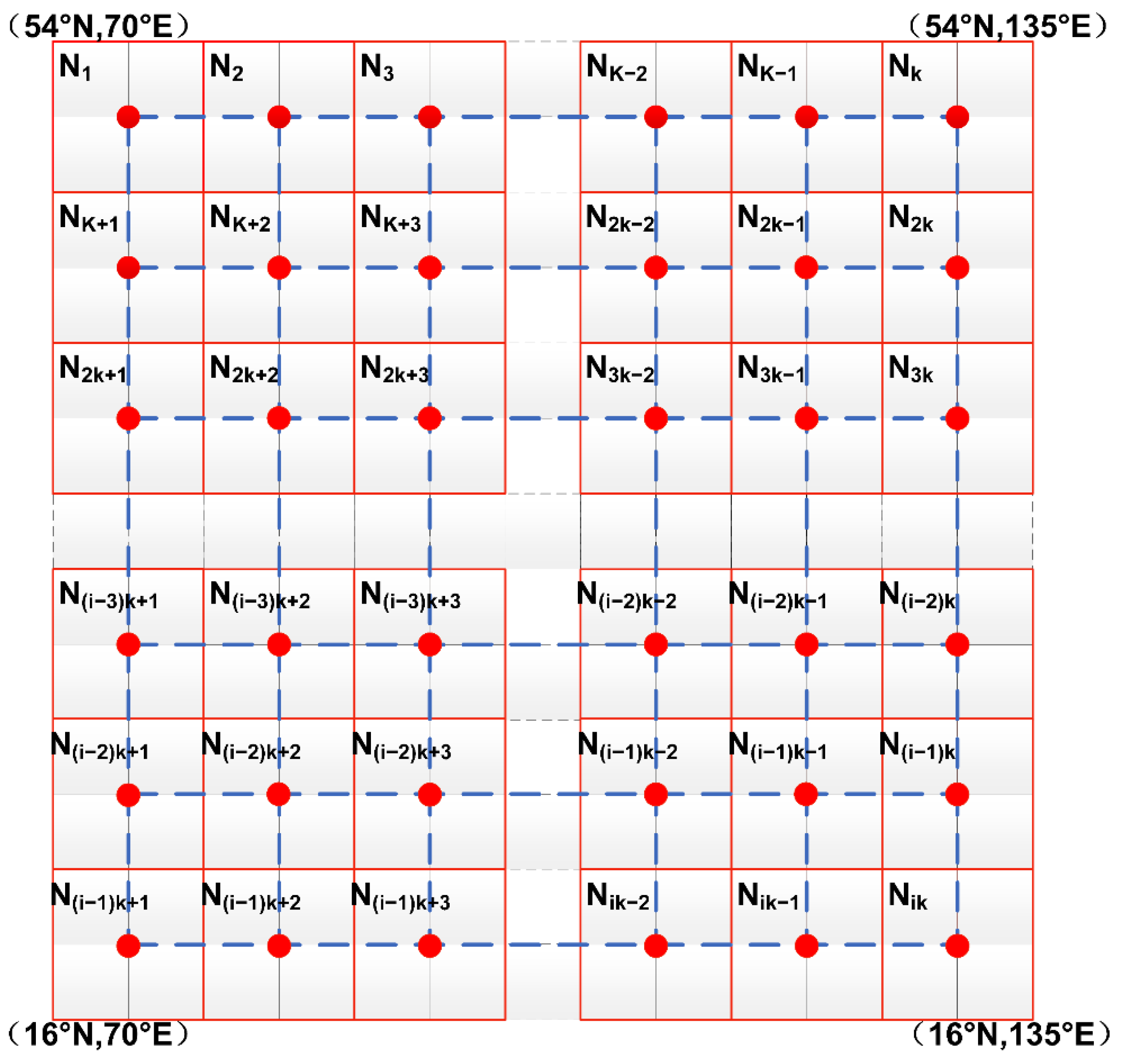
3. Development of the CTrop Model

Some shortcomings still exist in tropospheric models that have been developed, such as only single gridded data used for modeling. In this work, a sliding window algorithm is introduced to develop the tropospheric delay model, as shown in Figure 6. The new approach is instituted to divide the area of China into regular windows of the same size. Model parameters are estimated based on the data in each window to be taken as results of the center point of the sliding window. The realization process of the sliding window algorithm has been described in previous works [36,42].
As mentioned above, temperature, Tm, pressure, and water vapor pressure exhibit evident seasonal, latitudinal, and longitudinal characteristics over China, which should be taken into account to obtain a high-precision model. The equation in each window is expressed as follows:
M P ( φ , θ , D O Y ) = α 1 + α 2 · φ + α 3 · θ + α 4 · cos ( 2 π D O Y 365.25 ) + α 5 · sin ( 2 π D O Y 365.25 ) + α 6 · cos ( 4 π D O Y 365.25 ) + α 7 · sin ( 4 π D O Y 365.25 )
where M P is the meteorological parameters, such as temperature, Tm, pressure, and water vapor pressure; φ is the latitude; θ is the longitude; α 1 is the annual average value of the meteorological parameters; α 2 is the latitude correction; α 3 is the longitude correction; α 4 and α 5 are the annual amplitude coefficients of the meteorological parameters; α 6 and α 7 are the semiannual amplitude coefficients of the meteorological parameters, and D O Y is the day of the year.
The elevation of the grid points in the atmospheric reanalysis data is inconsistent with the elevation of GNSS stations. The height correction plays an important role in modeling, for which the lapse rates of meteorological parameters should be considered for height correction in the vertical dimension. The equation is written as follows:
L R ( φ , θ , D O Y ) = δ 1 + δ 2 · φ + δ 3 · θ + δ 4 · cos ( 2 π D O Y 365.25 ) + δ 5 · sin ( 2 π D O Y 365.25 ) + δ 6 · cos ( 4 π D O Y 365.25 ) + δ 7 · sin ( 4 π D O Y 365.25 )
where L R is the lapse rates of parameters in the vertical dimension, such as γ , β , λ , and τ ; δ 1 is the annual mean value of the lapse rate of parameters; δ 2 is the latitude correction; δ 3 is the longitude correction; δ 4 and δ 5 are the annual amplitude coefficients of the lapse rate parameters; δ 6 and δ 7 are the semiannual amplitude coefficients of the meteorological parameters.
The coefficients are calculated by least-squares adjustment in each window over China from 2012 to 2016, and a grid model calculating tropospheric key parameters over China named the CTrop model is established with a spatial resolution of 1.25 ° × 1 ° .
For horizontal interpolation, the inverse distance weighted and bilinear methods are commonly used. Considering the fact that changes in latitude have an impact on tropospheric parameters when developing the model, the inverse distance weighted method can reduce the impact on the interpolation results in the latitude direction, and grid points farther from the user have less of an impact on the interpolation, so the inverse distance weighted method is used for horizontal interpolation.
Only the day of the year (DOY) and the location of the station are needed when applying this model, which makes it very convenient. First, the four grid points nearest to the location are identified. The parameters of these four points at the height are then calculated. Finally, inverse distance weighted interpolation is employed to interpolate the required parameters at the given location.

4. Results and Discussion

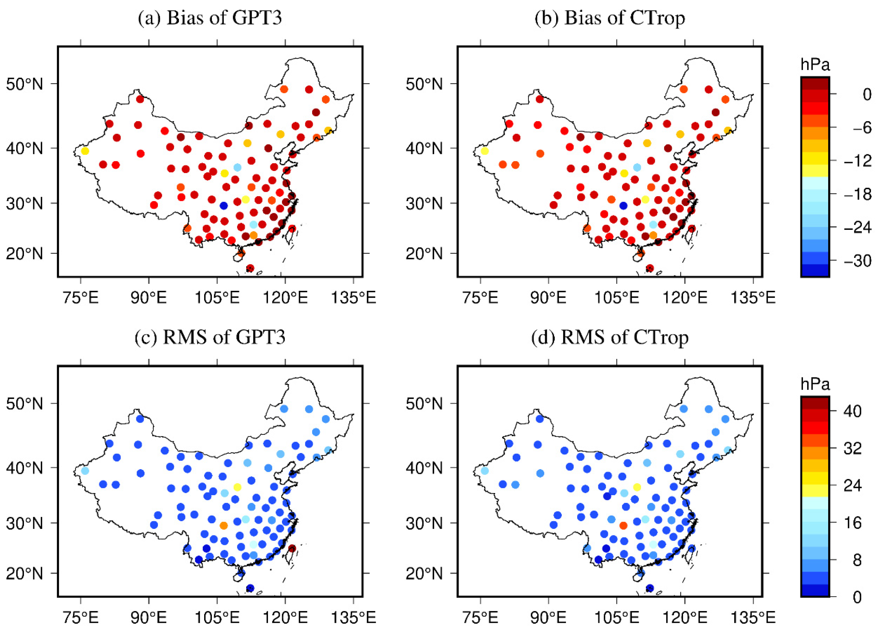
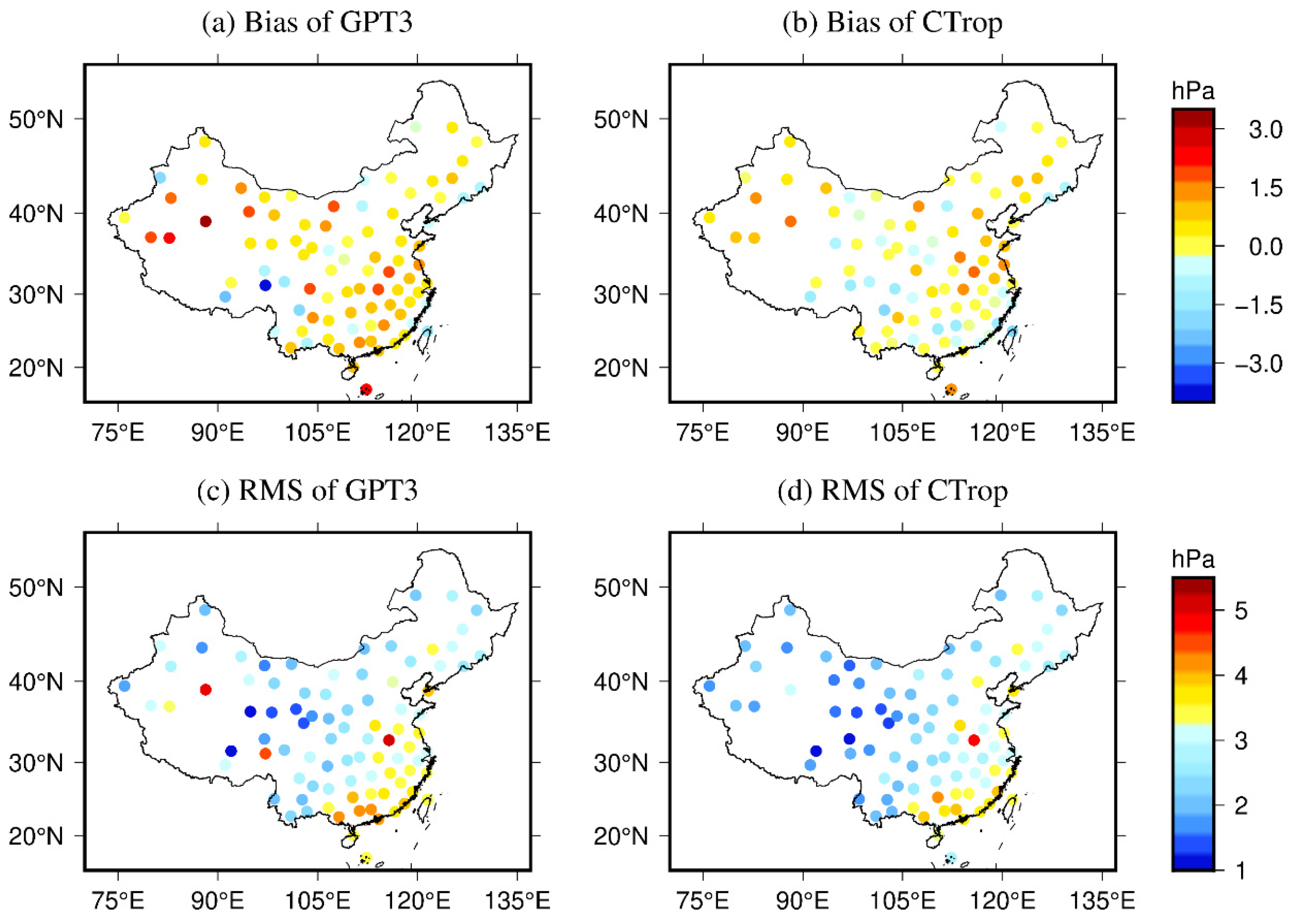
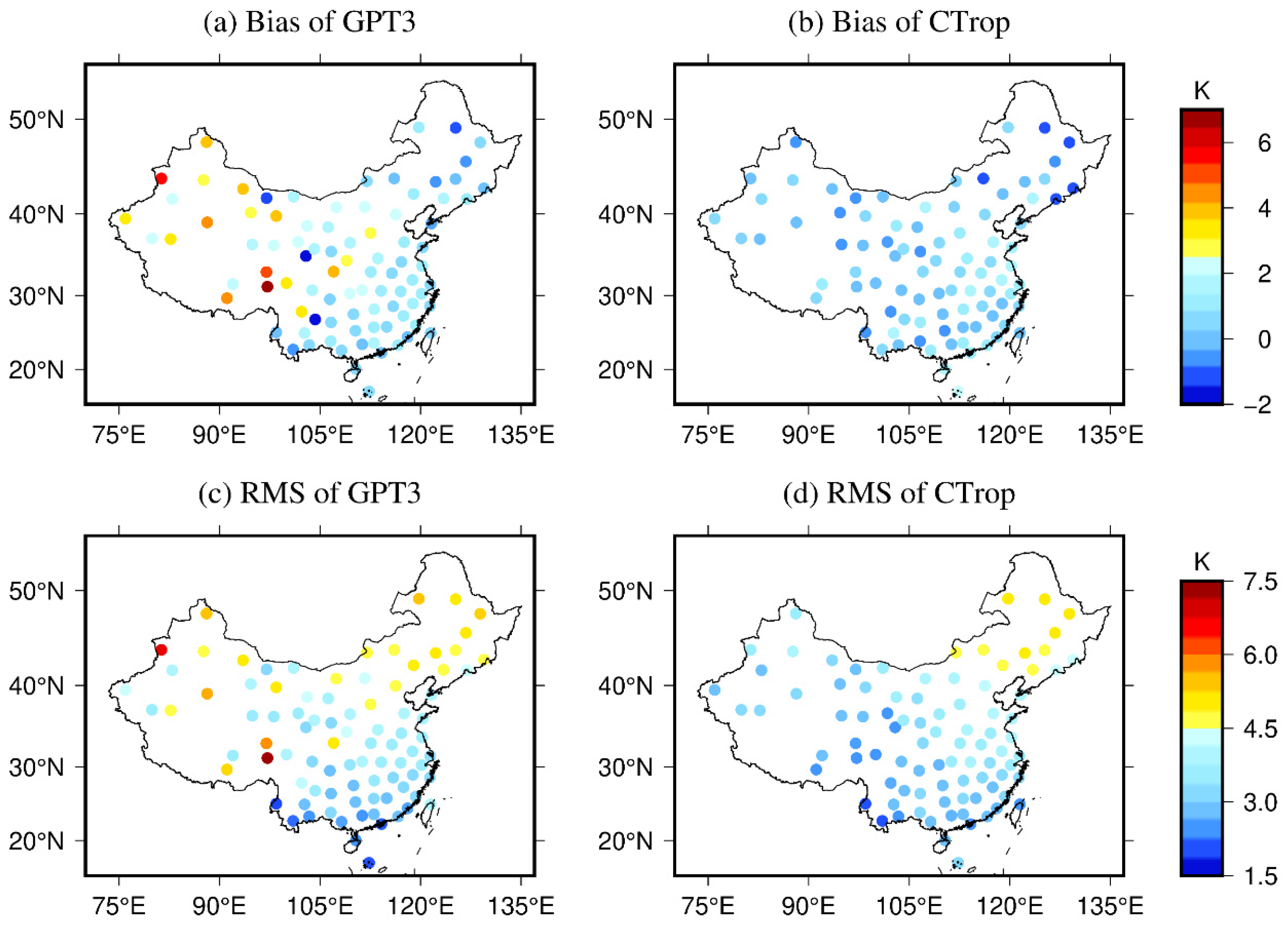
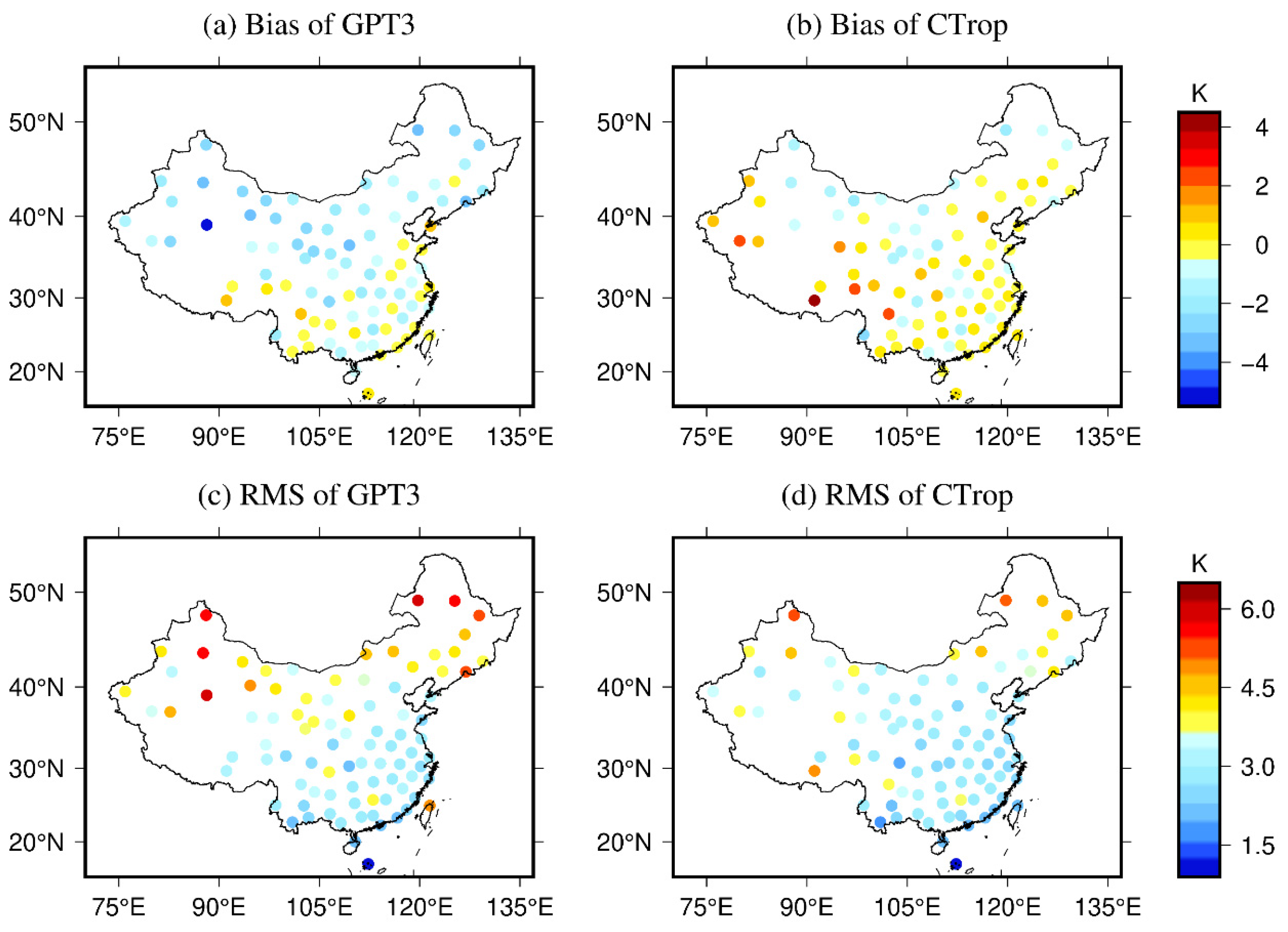
4.1. Analysis of the Accuracy of the CTrop Model

The performance of the CTrop model is validated by radiosonde data over China in 2017 compared with the GPT3 model at a resolution of 1° × 1°. The results are summarized in Table 1.
Table 1 lists the accuracy of the CTrop model for meteorological parameters in comparison with the GPT3 model. In terms of water vapor pressure, the RMS of the CTrop model is 2.60 hPa and is smaller than that of the GPT3 model, which decreases by 9%. As for pressure, both models reveal a negative bias. Although the CTrop model shows a larger bias than that of the GPT3 model, it attains a smaller RMS, which decreases by 6%. In terms of temperature, it also reveals a negative bias, which indicates that the value calculated by the CTrop and GPT3 model is smaller than that of the radiosonde data. The bias of the CTrop model is –0.11 K, which decreases by 91% compared to the GPT3 model. The performance of the CTrop model is superior to that of the GPT3 model, attaining an improvement of 10%. In terms of Tm, the CTrop model exhibits a smaller error than that of the GPT3 model. The bias of the CTrop model is 0.19 K and the RMS of the CTrop model is 3.35 K, with reductions of 87% and 13% compared with that of the GPT3 model, respectively.
To analyze the spatial characteristics of the performance of the CTrop and GPT3 models over China, the accuracy of the tropospheric parameters at each radiosonde site are calculated, and the results are shown in Figure 7, Figure 8, Figure 9 and Figure 10.
As can be observed in Figure 7, the overall distribution of performance of the pressure of the CTrop model is consistent with that of the GPT3 model over China, and the accuracy of both models is high in most radiosonde sites. The largest error of radiosonde sites for the CTrop model is the same as that of the GPT3 model. Furthermore, the performance of the CTrop model in the Taibei radiosonde site (25.03°N, 121.51°E) is better than that of the GPT3 model. Figure 8 shows that the GPT3 model attains the largest positive and negative bias in terms of water vapor pressure. The CTrop model shows a smaller RMS in the western area than in the eastern area. The performance of the CTrop and GPT3 models in the coastal areas is relatively low, the reason for which may be that the rainfall in the coastal areas is high, affected by the ocean climate. Figure 9 shows that both the GPT3 and CTrop models perform well in the southeast area for Tm over China while displaying large errors in the northeast region. The CTrop model attains a smaller error than that of the GPT3 model in the west area over China. Figure 10 shows that most stations show positive bias in the southeast area and negative bias in the northwest area. As the latitude increases, the RMS accuracy shows a downward trend. The CTrop model performs better in high latitude than does the GPT3 model. In short, the CTrop model shows better accuracy in estimating the tropospheric parameters than that of the GPT3 model.
The height of the radiosonde site is divided into three bands, and the performance at different heights of the CTrop and GPT3 models are calculated. The results are listed in Table 2. The precision of the two models is related to height. With the increase in height, the performance of pressure and water vapor pressure is improved, but the temperature decreases. The accuracy of the Tm of the CTrop model is improved with the increase in height, which is contrary to that of the GPT3 model.

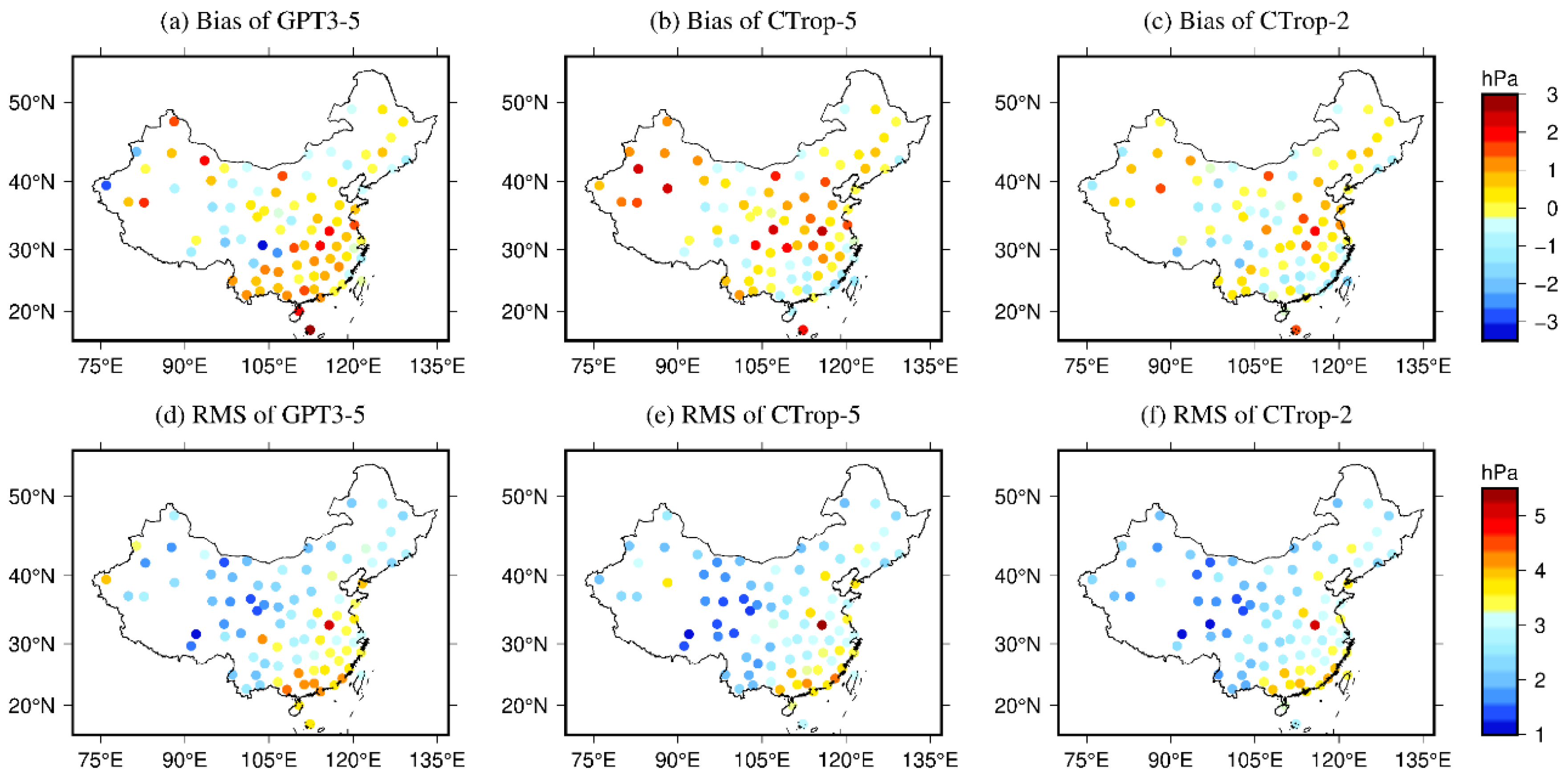
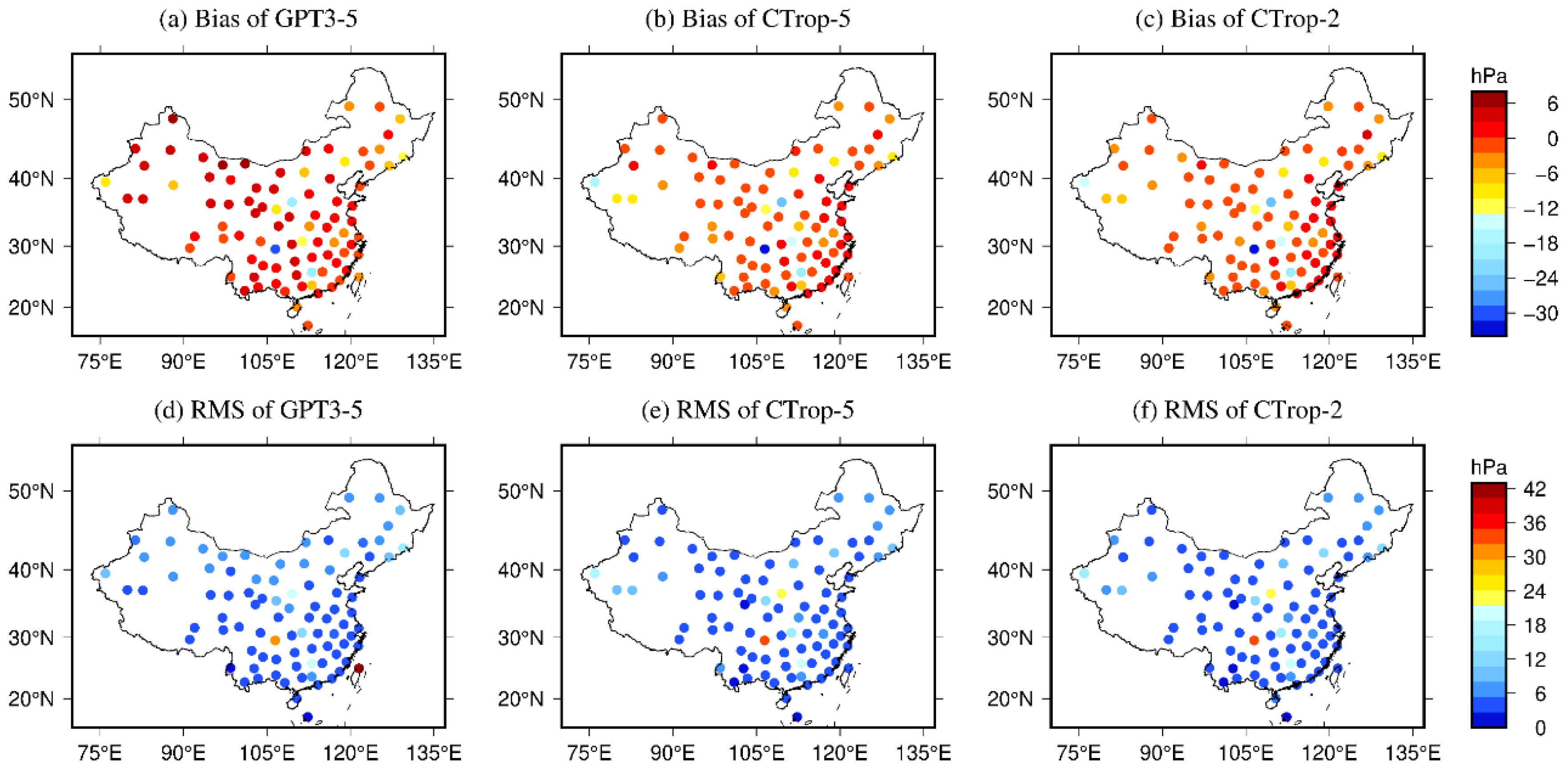
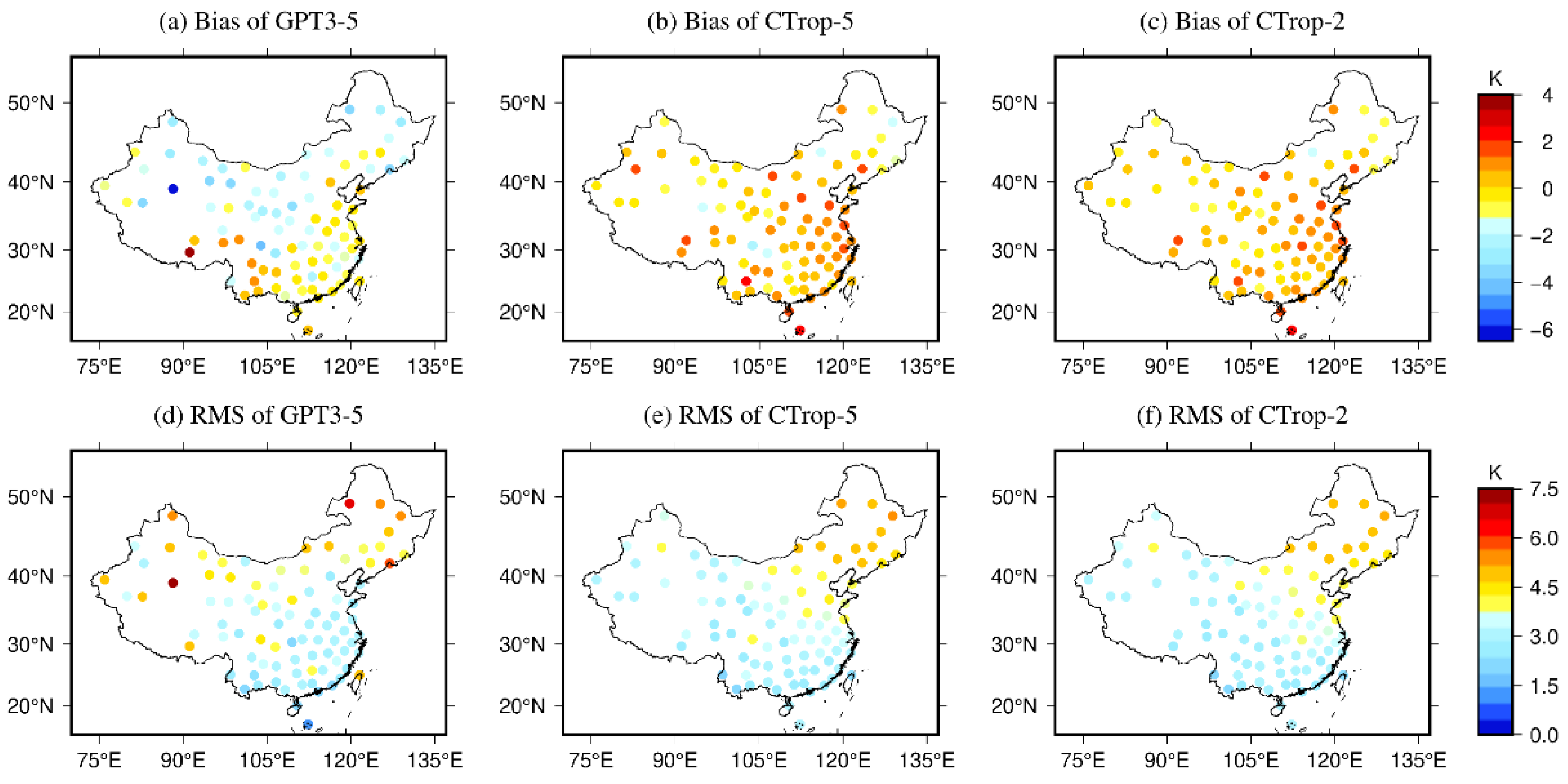
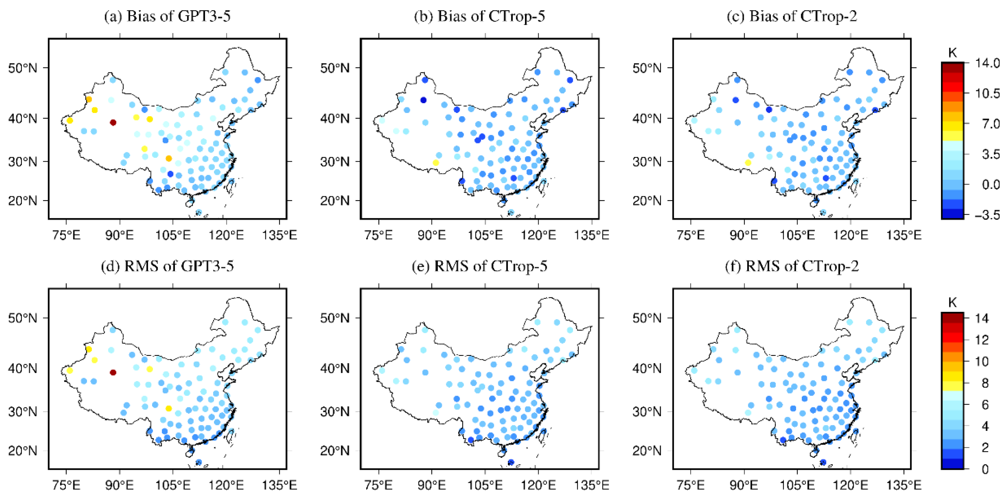
4.2. Analysis of the Accuracy of Different Resolutions of the CTrop Model

From the performance of the CTrop model compared with the GPT3 model, it can be observed that the CTrop model based on the sliding window algorithm performs superiorly to the GPT3 model. Since the resolutions of the GPT3 model are 1° × 1° and 5° × 5°, the applicability of the model is not sufficiently abundant. Based on the sliding window algorithm, users can access model parameters of different resolutions for their requirements, which represents one of its advantages. The goal behind the development of a lower horizontal resolution version of the CTrop model is the reduction in the amount of gridded data provided to users, as well as speeding up the troposphere delay computation process.
To analyze the influence of different resolutions of the CTrop model, window sizes of 2.5° × 2° and 5° × 4° (lon. × lat.) are proposed for the development of models, named CTrop-2 and CTrop-5, respectively. The CTrop model with sparser grids is compared to the 5-degree horizontal resolution version of the GPT3 model, named the GPT3-5 model. In view of the high resolution of the CTrop-2 model, the discussion is limited to the CTrop-5 versus the GPT3-5 model, and the result of the CTrop-2 model is only displayed without discussion. The results are shown in Table 3 and Table 4 and Figure 11, Figure 12, Figure 13 and Figure 14.
Table 3 and Table 4 indicate that as the spatial resolution of the CTrop model decreases, the accuracy gradually decreases. The Ctrop model also has better accuracy than the GPT3-5 model in lower spatial resolution. Regarding the water vapor pressure, the RMS of the Ctrop-5 model is 2.71 hPa, showing an improvement of 5% compared with the GPT3-5 model. Considering the pressure, the CTrop-5 model achieves accuracy improvements of 10% when compared to the GPT3-5 model. Regarding temperature, the bias of the CTrop-5 model appears as a negative value, while the GPT3-5 model displays a positive value. The RMS of the CTrop-5 model is 3.26 K, showing an improvement of 22% when compared with the GPT3-5 model. In terms of Tm, the precision of the CTrop-5 model is 3.43 K, also presenting a slight improvement when compared with the GPT3-5 model.
Figure 11 shows that all models display a large RMS of water vapor pressure in the southeast of China. The CTrop-5 model shows an accuracy improvement in the northeast of China when compared with the GPT3-5 model. Both models show large errors in the southeast of China, which is subject to subtropical monsoons. Water vapor is transported by monsoons from the sea to these areas, resulting in a higher error for modeling [12]. Figure 12 shows that the CTrop-5 model and the GPT3-5 model present positive and negative biases of pressure in the majority of China. The CTrop-5 model presents a slight improvement at a few stations in the northeast of China when compared with the GPT3-5 model. Figure 13 shows that all models have better accuracy of Tm in the south of China than in the north of China. The CTrop-5 model presents an improvement in the west of China when compared with the GPT3-5 model. Figure 14 shows that the CTrop-5 model has better accuracy in the west of China than that of the GPT3-5 model. Consequently, the lower horizontal resolution version of the CTrop model shows better accuracy in estimating the tropospheric parameters than that of the GPT3 model.

5. Conclusions

In this work, the distribution characteristics of meteorological parameters are analyzed, and it is observed that the meteorological parameters exhibit major annual and semiannual periodic variations that are also related to latitude and longitude. Considering the spatial distribution and time-varying characteristics of the meteorological parameters, a refined regional empirical model (CTrop) based on the sliding window algorithm is developed for the estimation of tropospheric key parameters over China. Only the day of the year (DOY) and the location of the station are needed when applying this model, which makes it very convenient. The performance of the CTrop and GPT3 models are validated by radiosonde data. Validation results demonstrate that the CTrop model shows higher precision than that of the GPT3 model in all meteorological parameters. The improvements are 6%, 10%, 9%, and 13% for pressure, temperature, water vapor pressure, and weighted mean temperature, respectively. Three different resolutions of the CTrop model are also developed based on the sliding window algorithm, for which users can access model parameters of different resolutions for their requirements to reduce the amount of gridded data provided to the users, as well as to speed up the troposphere delay computation process. The results demonstrate that the CTrop model realizes better performance than that of the GPT3 model over China, which can meet the needs for GNSS meteorology and GNSS positioning. Although the CTrop model is only developed in regions over China with the aim of meeting the needs for GNSS positioning in China, we intend to expand the model to a global model in future work.

Author Contributions

Conceptualization, L.H. (Liangke Huang) and L.L.; methodology, G.Z. and L.H. (Liangke Huang); validation, C.L., L.H. (Liangke Huang) and L.Z.; formal analysis, G.Z.; writing—original draft preparation, G.Z. and C.L.; writing—review and editing, L.H. (Liangke Huang), J.L., L.H. (Ling Huang) and H.H.; funding acquisition, L.H. (Liangke Huang) and L.L. All authors have read and agreed to the published version of the manuscript.

Funding

This work was sponsored by the National Natural Foundation of China (41864002; 41704027); Guangxi Natural Science Foundation of China (2018GXNSFAA281182; 2020GXNSFBA297145; 2018GXNSFAA281279; 2020GXNSFBA159033); Innovation Project of Guangxi Graduate Education (YCSW2021209); Guangxi Science and Technology Base and Talent Project (AD19245060); The Guangxi Key Laboratory of Spatial Information and Geomatics (19-050-11-24), and the “Ba Gui Scholars” program of the provincial government of Guangxi.

Institutional Review Board Statement

Not applicable.

Informed Consent Statement

Not applicable.

Data Availability Statement

The MERRA-2 data can be freely accessed at https://goldsmr4.gesdisc.eosdis.nasa.gov/data/MERRA2/ (accessed on 16 May 2020). The radiosonde data can be accessed at http://www1.ncdc.noaa.gov/pub/data/igra/ (accessed on 16 May 2020). The parameters of the CTrop model, as well as codes, are available upon request to Liangke Huang ([email protected]).

Acknowledgments

The authors would like to thank NASA for providing the MERRA-2 grid data and IGRA (Integrated Global Radiosonde Archive) for providing the radiosonde data in this study.

Conflicts of Interest

The authors declare no conflict of interest.

References

  1. Saastamoinen, J. Contributions to the theory of atmospheric refraction. Bull. Géodésique 1972, 105, 279–298. [Google Scholar] [CrossRef]
  2. Guo, J.; Hou, R.; Zhou, M.; Jin, X.; Li, C.; Liu, X.; Gao, H. Monitoring 2019 Forest Fires in Southeastern Australia with GNSS Technique. Remote Sens. 2021, 13, 386. [Google Scholar] [CrossRef]
  3. Boutiouta, S.; Lahcene, A. Preliminary study of GNSS meteorology techniques in Algeria. Int. J. Remote Sens. 2013, 34, 5105–5118. [Google Scholar] [CrossRef]
  4. Tunalı, E.; Özlüdemir, M.T. GNSS PPP with different troposphere models during severe weather conditions. GPS Solut. 2019, 23, 82. [Google Scholar] [CrossRef]
  5. Li, Z.; Wen, Y.; Zhang, P.; Liu, Y.; Zhang, Y. Joint Inversion of GPS, Leveling, and InSAR Data for the 2013 Lushan (China) Earthquake and Its Seismic Hazard Implications. Remote Sens. 2020, 12, 715. [Google Scholar] [CrossRef] [Green Version]
  6. Ning, T.; Wickert, J.; Deng, Z.; Heise, S.; Dick, G.; Vey, S.; Schöne, T. Homogenized time series of the atmospheric water vapor content obtained from the GNSS reprocessed data. J. Clim. 2016, 29, 2443–2456. [Google Scholar] [CrossRef]
  7. Hopfield, H.S. Two-Quartic tropospheric refractivity profile for correcting satellite data. J. Geophys. Res. 1969, 74, 4487–4499. [Google Scholar] [CrossRef]
  8. Black, H.D. An easily implemented algorithm for the tropospheric range correction. J. Geophys. Res. 1978, 83, 1825–1828. [Google Scholar] [CrossRef]
  9. Lu, C.; Li, X.; Cheng, J.; Dick, G.; Ge, M.; Wickert, J.; Schuh, H. Real-time tropospheric delay retrieval from multi-GNSS PPP ambiguity resolution: Validation with final troposphere products and a numerical weather model. Remote Sens. 2018, 10, 481. [Google Scholar] [CrossRef] [Green Version]
  10. Cao, L.; Zhang, B.; Li, J.; Yao, Y.; Liu, L.; Ran, Q.; Xiong, Z. A Regional Model for Predicting Tropospheric Delay and Weighted Mean Temperature in China Based on GRAPES_MESO Forecasting Products. Remote Sens. 2021, 13, 2644. [Google Scholar] [CrossRef]
  11. Li, T.; Wang, L.; Chen, R.; Fu, W.; Xu, B.; Jiang, P.; Liu, J.; Zhou, H.; Han, Y. Refining the empirical global pressure and temperature model with the ERA5 reanalysis and radiosonde data. J. Geod. 2021, 95, 31. [Google Scholar] [CrossRef]
  12. Wu, M.; Jin, S.; Li, Z.; Cao, Y.; Ping, F.; Tang, X. High-Precision GNSS PWV and Its Variation Characteristics in China Based on Individual Station Meteorological Data. Remote Sens. 2021, 13, 1296. [Google Scholar] [CrossRef]
  13. Zhang, W.; Lou, Y.; Huang, J.; Liu, W. A refined regional empirical pressure and temperature model over China. Adv. Space Res. 2018, 62, 1065–1074. [Google Scholar] [CrossRef]
  14. Li, J.; Zhang, B.; Yao, Y.; Liu, L.; Sun, Z.; Yan, X. A Refined Regional Model for Estimating Pressure, Temperature, and Water Vapor Pressure for Geodetic Applications in China. Remote Sens. 2020, 12, 1713. [Google Scholar] [CrossRef]
  15. Huang, L.; Liu, L.; Yao, C. A zenith tropospheric delay correction model based on the regional CORS network. Geod. Geodyn. 2012, 3, 53–62. [Google Scholar]
  16. Huang, L.; Xie, S.; Liu, L.; Li, J.; Chen, J.; Kang, C. SSIEGNOS: A New Asian Single Site Tropospheric Correction Model. ISPRS Int. J. Geo-Inf. 2017, 6, 20. [Google Scholar] [CrossRef] [Green Version]
  17. Leandro, R.F.; Santos, M.C.; Langley, R.B. UNB neutral atmosphere models: Development and performance. In Proceedings of the ION NTM 2006, Monterey, CA, USA, 18–20 January 2006; pp. 564–573. [Google Scholar]
  18. Leandro, R.F.; Langley, R.B.; Santos, M.C. UNB3m_pack: A neutral atmosphere delay package for radiometric space techniques. GPS Solut. 2008, 12, 65–70. [Google Scholar] [CrossRef]
  19. Penna, N.; Dodson, A.; Chen, W. Assessment of EGNOS tropospheric correction model. J. Navig. 2001, 54, 37–55. [Google Scholar] [CrossRef] [Green Version]
  20. Krueger, E.; Schüler, T.; Hein, G.; Martellucci, A.; Blarzino, G. Galileo tropospheric correction approaches developed within GSTB-V1. In Proceedings of the ENC-GNSS 2004, Rotterdam, The Netherlands, 16–19 May 2004. [Google Scholar]
  21. Schüler, T. The TropGrid2 standard tropospheric correction model. GPS Solut. 2014, 18, 123–131. [Google Scholar] [CrossRef]
  22. Böhm, J.; Heinkelmann, R.; Schuh, H. Short note: A global model of pressure and temperature for geodetic applications. J. Geod. 2007, 81, 679–683. [Google Scholar] [CrossRef]
  23. Lagler, K.; Schindelegger, M.; Böhm, J.; Krásná, H.; Nilsson, T. GPT2: Empirical Slant Delay Modelfor Radio Space Geodetic Techniques. Geophys. Res. Lett. 2013, 40, 1069–1073. [Google Scholar] [CrossRef] [PubMed] [Green Version]
  24. Böhm, J.; Möller, G.; Schindelegger, M.; Pain, G.; Weber, R. Development of an improved blind model for slant delays in the troposphere (GPT2w). GPS Solut. 2015, 19, 433. [Google Scholar] [CrossRef] [Green Version]
  25. Landskron, D.; Böhm, J. VMF3/GPT3: Refined discrete and empirical troposphere mapping functions. J. Geod. 2018, 92, 349–360. [Google Scholar] [CrossRef]
  26. Ding, J.; Chen, J. Assessment of Empirical Troposphere Model GPT3 Based on NGL’s Global Troposphere Products. Sensors 2020, 20, 3631. [Google Scholar] [CrossRef]
  27. Sun, Z.Y.; Zhang, B.; Yao, Y.B. An ERA5-based model for estimating tropospheric delay and weighted mean temperature over China with improved spatiotemporal resolutions. Earth Space Sci. 2019, 6, 1926–1941. [Google Scholar] [CrossRef]
  28. Gui, K.; Che, H.; Chen, Q.; Zeng, Z.; Liu, H.; Wang, Y.; Zheng, Y.; Sun, T.; Liao, T.; Wang, H.; et al. Evaluation of radiosonde, MODIS-NIR-Clear, and AERONET precipitable water vapor using IGS ground-based GPS measurements over China. Atmos Res. 2017, 197, 461–473. [Google Scholar] [CrossRef]
  29. Randles, C.A.; Da Silva, A.M.; Buchard, V.; Colarco, P.R.; Darmenov, A.; Govindaraju, R.; Smirnov, A.; Holben, B.; Ferrare, R.; Hair, J.; et al. The MERRA-2 Aerosol Reanalysis, 1980 Onward. Part I: System Description and Data Assimilation Evaluation. J. Clim. 2017, 30, 6823–6850. [Google Scholar] [CrossRef]
  30. Gelaro, R.; McCarty, W.; Suárez, M.J.; Todling, R.; Molod, A.; Takacs, L.; Randles, C.A.; Darmenov, A.; Bosilovich, M.G.; Reichle, R.; et al. The Modern-Era Retrospective Analysis for Research and Applications, Version 2 (MERRA-2). J. Clim. 2017, 30, 5419–5454. [Google Scholar] [CrossRef]
  31. Molod, A.; Takacs, L.; Suarez, M.; Bacmeister, J. Development of the GEOS-5 atmospheric general circulation model: Evolution from MERRA to MERRA2. Geosci. Model Dev. 2015, 8, 1339–1356. [Google Scholar] [CrossRef] [Green Version]
  32. Kleist, D.T.; Parrish, D.F.; Derber, J.C.; Treadon, R.; Errico, R.M.; Yang, R. Improving incremental balance in the GSI 3DVAR analysis system. Mon. Weather. Rev. 2009, 137, 1046–1060. [Google Scholar] [CrossRef]
  33. Wu, W.S.; Purser, R.J.; Parrish, D.F. Three-dimensional variational analysis with spatially inhomogeneous covariances. Mon. Weather. Rev. 2002, 130, 2905–2916. [Google Scholar] [CrossRef] [Green Version]
  34. Gupta, P.; Verma, S.; Bhatla, R.; Chandel, A.S.; Singh, J.; Payra, S. Validation of surface temperature derived from MERRA-2 Reanalysis against IMD gridded data set over India. Earth Space Sci. 2020, 7, e2019EA000910. [Google Scholar] [CrossRef] [Green Version]
  35. Huang, L.; Mo, Z.; Liu, L.; Zeng, Z.; Chen, J.; Xiong, S.; He, H. Evaluation of hourly PWV products derived from ERA5 and MERRA-2 over the Tibetan Plateau using ground-based GNSS observations by two enhanced models. Earth Space Sci. 2021, 8, e2020EA001516. [Google Scholar] [CrossRef]
  36. Huang, L.K.; Jiang, W.P.; Liu, L.L.; Chen, H.; Ye, S.R. A new global grid model for the determination of atmospheric weighted mean temperature in GPS precipitable water vapor. J. Geod. 2019, 93, 159–176. [Google Scholar] [CrossRef]
  37. Yao, Y.B.; Zhang, B.; Xu, C.Q.; Chen, J.J. Analysis of the global T m-T s correlation and establishment of the latitude-related linear model. Chin. Sci. Bull. 2014, 59, 2340–2347. [Google Scholar] [CrossRef]
  38. Bevis, M.; Businger, S.; Herring, T.A.; Rocken, C.; Anthes, R.; Ware, R.H. GPS meteorology: Remote sensing of atmospheric water vapor using the Global Positioning System. J. Geophys. Res. 1992, 97, 15787–15801. [Google Scholar] [CrossRef]
  39. Bevis, M.; Businger, S.; Chiswell, S.; Herring, T.A.; Anthes, R.A.; Rocken, C.; Ware, R.H. GPS meteorology: Mapping zenith wet delays onto precipitable water. J. Appl. Meteorol. 1994, 33, 379–386. [Google Scholar] [CrossRef]
  40. Yao, Y.B.; Xu, C.Q.; Shi, J.B.; Cao, N.; Zhang, B.; Yang, J.J. ITG: A New Global GNSS Tropospheric Correction Model. Sci. Rep. 2015, 5, 10273. [Google Scholar] [CrossRef] [Green Version]
  41. Askne, J.; Nordius, H. Estimation of tropospheric delay for microwaves from surface weather data. Radio Sci. 1987, 22, 379–386. [Google Scholar] [CrossRef]
  42. Huang, L.K.; Zhu, G.; Liu, L.L.; Chen, H.; Jiang, W.P. A global grid model for the correction of the vertical zenith total delay based on a sliding window algorithm. GPS Solut. 2021, 25, 98. [Google Scholar] [CrossRef]
Figure 1. Distribution of 89 radiosonde stations over China. Blue dots are radiosonde stations, and red triangles are representative grid points.
Remotesensing 13 03546 g001
Figure 2. Relationships between temperature and geopotential height at four MERRA-2 grid points over China in 2016: (a) 42°N, 90°E; (b) 42°N, 120°E; (c) 30°N, 90°E; (d) 30°N, 120°E. Blue dots are the temperature of MERRA-2 in each height, and red lines are the linear fit to them.
Remotesensing 13 03546 g002
Figure 3. Time series of tropospheric parameters for pressure (a), parameters for water vapor pressure (b), parameters for temperature (c), and parameters for Tm (d) provided by MERRA-2 data from 2012 to 2016. The dots shown are the mean values of each latitude interval for each epoch. Blue dots are at high latitude, green dots are at middle latitude, red dots are at low latitude, and orange dots are the mean value.
Remotesensing 13 03546 g003
Figure 4. Distribution of the annual mean of the tropospheric parameters for pressure (a), parameters for water vapor pressure (b), parameters for temperature (c), and parameters for Tm (d) calculated from MERRA-2 data.
Remotesensing 13 03546 g004
Figure 5. Distribution of the annual mean of the lapse rate for pressure (a), decrease factor for water vapor pressure (b), lapse rate for temperature (c), and lapse rate for Tm (d).
Remotesensing 13 03546 g005
Figure 6. Realization process of the sliding window algorithm over China. The red rectangles denote the size of the sliding windows, and the red dots denote the center point of each window. The new grid over China consists of red dots and blue dashed lines.
Remotesensing 13 03546 g006
Figure 7. Distribution of the performance of pressure at each radiosonde site in 2017 by the CTrop and GPT3 models: (a) Bias of GPT3; (b) Bias of CTrop; (c) RMS of GPT3; (d) RMS of CTrop. The positive bias means the model outputs are larger than the reference values, while the negative bias means they are smaller than the reference values.
Remotesensing 13 03546 g007
Figure 8. Distribution of the performance of water vapor pressure at each radiosonde site in 2017 by the CTrop and GPT3 models: (a) Bias of GPT3; (b) Bias of CTrop; (c) RMS of GPT3; (d) RMS of CTrop.
Remotesensing 13 03546 g008
Figure 9. Distribution of the performance of Tm at each radiosonde site in 2017 by the CTrop and GPT3 models: (a) Bias of GPT3; (b) Bias of CTrop; (c) RMS of GPT3; (d) RMS of CTrop.
Remotesensing 13 03546 g009
Figure 10. Distribution of the performance of temperature at each radiosonde site in 2017 by the CTrop and GPT3 models: (a) Bias of GPT3; (b) Bias of CTrop; (c) RMS of GPT3; (d) RMS of CTrop.
Remotesensing 13 03546 g010
Figure 11. Distribution of the performance of water vapor pressure in different resolutions of the CTrop and GPT3 models validated by radiosonde sites in 2017: (a) Bias of GPT3-5; (b) Bias of CTrop-5; (c) Bias of CTrop-2; (d) RMS of GPT3-5; (e) RMS of CTrop-5; (f) RMS of CTrop-2. The positive bias means the model outputs are larger than the reference values, while the negative bias means they are smaller than the reference values.
Remotesensing 13 03546 g011
Figure 12. Distribution of the performance of pressure in different resolutions of the CTrop and GPT3 models validated by radiosonde sites in 2017: (a) Bias of GPT3-5; (b) Bias of CTrop-5; (c) Bias of CTrop-2; (d) RMS of GPT3-5; (e) RMS of CTrop-5; (f) RMS of CTrop-2.
Remotesensing 13 03546 g012
Figure 13. Distribution of the performance of Tm in different resolutions of the CTrop and GPT3 models validated by radiosonde sites in 2017: (a) Bias of GPT3-5; (b) Bias of CTrop-5; (c) Bias of CTrop-2; (d) RMS of GPT3-5; (e) RMS of CTrop-5; (f) RMS of CTrop-2.
Remotesensing 13 03546 g013
Figure 14. Distribution of the performance of temperature in different resolutions of the CTrop and GPT3 models validated by radiosonde sites in 2017: (a) Bias of GPT3-5; (b) Bias of CTrop-5; (c) Bias of CTrop-2; (d) RMS of GPT3-5; (e) RMS of CTrop-5; (f) RMS of CTrop-2.
Remotesensing 13 03546 g014
Table 1. Accuracy statistics of the meteorological parameters at each radiosonde site by the CTrop and GPT3 models.
ModelCTrop/GPT3
Parameterse (hPa)P (hPa)T (K)Tm (K)
biasmean0.01/0.34–2.35/–2.12–0.11/–1.250.19/1.46
min–2.08/–3.83–31.67/–31.72–2.43/–5.03–0.94/–1.89
max1.59/3.192.14/2.734.15/1.162.31/6.75
RMSmean2.60/2.865.51/5.833.09/3.443.35/3.87
min1.04/1.091.86/2.041.12/1.002.04/1.88
max4.83/5.0632.07/42.715.15/6.015.02/7.27
Table 2. Statistics of performance at different heights of the CTrop and GPT3 models validated by radiosonde data.
ModelCTrop/GPT3
Height (m)e (hPa)P (hPa)T (K)Tm (K)
bias<5000.07/0.47–2.18/–2.05–0.11/–0.880.53/0.88
500~20000.04/0.45–3.57/2.50–0.37/–1.940.19/1.99
>2000–0.38/–0.57–0.91/–1.210.81/–0.800.13/2.45
RMS<5003.20/3.295.69/6.552.84/3.153.48/3.61
500~20002.09/2.475.96/5.513.32/3.913.37/4.13
>20001.50/2.023.14/3.463.43/3.322.67/4.32
Table 3. Statistics of the bias of different resolutions of the CTrop model compared with the GPT3-5 model.
Modelse (hPa)P (hPa)T (K)Tm (K)
Mean [Min, Max]
CTrop-2–0.03
[–1.87, 2.01]
–2.83
[–32.94, 2.79]
–0.05
[–2.85, 5.04]
0.27
[–1.32, 2.39]
CTrop-50.32
[–1.69, 2.53]
–2.78
[–33.17, 2.38]
–0.15
[–3.25, 5.86]
0.30
[–2.32, 2.46]
GPT3-50.16
[–3.45, 2.84]
–0.46
[–29.90, 6.44]
1.76
[–2.22, 13.77]
–1.19
[–6.14, 3.77]
Table 4. Statistic of the RMS of different resolutions of the CTrop model compared with the GPT3-5 model.
Modelse (hPa)P (hPa)T (K)Tm (K)
Mean [Min, Max]
CTrop-22.64
[1.08, 5.02]
5.59
[2.00, 33.15]
3.16
[1.17, 5.72]
3.37
[1.82, 5.11]
CTrop-52.71
[1.13, 5.34]
5.61
[2.00, 33.36]
3.26
[1.24, 6.41]
3.43
[1.87, 5.28]
GPT3-52.84
[1.05, 5.10]
6.18
[1.77, 42.89]
4.20
[2.15, 14.18]
3.52
[1.03, 7.37]
Publisher’s Note: MDPI stays neutral with regard to jurisdictional claims in published maps and institutional affiliations.

