
Modifications of the Multi-Layer Perceptron for Hyperspectral Image Classification


School of Electronics and Information Engineering, Harbin Institute of Technology, Harbin 150001, China
*
Author to whom correspondence should be addressed.
Remote Sens. 2021, 13(17), 3547; https://0-doi-org.brum.beds.ac.uk/10.3390/rs13173547
Submission received: 22 July 2021
/
Revised: 1 September 2021
/
Accepted: 2 September 2021
/
Published: 6 September 2021
(This article belongs to the Special Issue Spectral Data Meets Machine Learning: From Datasets to Algorithms and Applications)
Abstract
:Recently, many convolutional neural network (CNN)-based methods have been proposed to tackle the classification task of hyperspectral images (HSI). In fact, CNN has become the de-facto standard for HSI classification. It seems that the traditional neural networks such as multi-layer perceptron (MLP) are not competitive for HSI classification. However, in this study, we try to prove that the MLP can achieve good classification performance of HSI if it is properly designed and improved. The proposed Modified-MLP for HSI classification contains two special parts: spectral–spatial feature mapping and spectral–spatial information mixing. Specifically, for spectral–spatial feature mapping, each input sample of HSI is divided into a sequence of 3D patches with fixed length and then a linear layer is used to map the 3D patches to spectral–spatial features. For spectral–spatial information mixing, all the spectral–spatial features within a single sample are feed into the solely MLP architecture to model the spectral–spatial information across patches for following HSI classification. Furthermore, to obtain the abundant spectral–spatial information with different scales, Multiscale-MLP is proposed to aggregate neighboring patches with multiscale shapes for acquiring abundant spectral–spatial information. In addition, the Soft-MLP is proposed to further enhance the classification performance by applying soft split operation, which flexibly capture the global relations of patches at different positions in the input HSI sample. Finally, label smoothing is introduced to mitigate the overfitting problem in the Soft-MLP (Soft-MLP-L), which greatly improves the classification performance of MLP-based method. The proposed Modified-MLP, Multiscale-MLP, Soft-MLP, and Soft-MLP-L are tested on the three widely used hyperspectral datasets. The proposed Soft-MLP-L leads to the highest OA, which outperforms CNN by 5.76%, 2.55%, and 2.5% on the Salinas, Pavia, and Indian Pines datasets, respectively. The obtained results reveal that the proposed models provide competitive results compared to the state-of-the-art methods, which shows that the MLP-based methods are still competitive for HSI classification.
1. Introduction
Hyperspectral sensors are able to capture hyperspectral image (HSI) with abundant spectral and spatial information, which could accurately characterize and identify different land-covers. The valuable source of the rich information makes the HSI useful in a wide range of applications, including agriculture (e.g., crops classification [1] and detection of water quality conditions [2]), the food industry (e.g., characterizing product quality [3]), water and maritime resources management (e.g., water quality analysis [4] and sea ice detection [5]), forestry and environmental management (e.g., health of forests [6] and infestations in plantation forestry [7]), security and defense applications (e.g., identification of man-made materials [8]), and vision technology (e.g., 3D reconstruction [9] and image detection [10]).
HSI classification refers to a task of assigning a category to each pixel in the scene. Due to the fact that it is a basic procedure in many applications, HSI classification is a fundamental and hot topic in the remote sensing community [11].
A large number of methods have been proposed for HSI classification and most of them are supervised learning-based methods [12]. There are two important parts for accurate HSI classification: discriminative feature extraction and robust classifier. For feature extraction of HSI, many morphological operations, including morphological profiles (MPs) [13], extended MPs (EMPs) [14], extended multi-attribute profile (EMAP) [15], and extinction profiles (EPs) [16], have been developed to extract the HSI features. For a robust classifier of HSI, due to its low sensitivity to high dimensionality, support vector machine (SVM) was widely used as a good classifier [17].
Recently, various studies applied for HSI classification have demonstrated the success of deep learning-based methods, such as stacked auto-encoder [18] and deep belief network [19]. Moreover, recurrent neural network has promising performance in learning hyperspectral image with sequential data [20]. Among the deep learning-based methods for HSI classification, convolutional neural network (CNN) with the local-connection and shared-weight architecture has become the mainstream approach for classifying HSI [21].
Depending on the input information of models, the HSI classification methods based on the CNN methods can be divided into three types: the spectral CNN, spatial CNN, and spectral–spatial CNN [22]. The spectral CNN-based approaches adopted CNN on the spectral of HSI to extract discriminative spectral features. For instance, in [23], the spectral information of each pixel is extracted by the CNN with only five convolutional layers. Besides, Li et al. presented a novel pixel-pairs strategy for HSI classification by utilizing the deep CNN, which provides excellent performance [24].
The second type of CNN-based approaches for HSI classification is named the spatial CNN. Since there exist amounts of spatial information in the HSI, the 2D convolution layer is designed in many studies to extract the spatial features of HSI from a local cube in the spatial domain [25,26,27]. For instance, in [27], principal component analysis was first applied to reduce the dimension of the HSI, then, 2D convolution layer was utilized to extract the spatial features of fixed neighborhood of each pixel.
The last type based on the CNN for classifying HSI is called the spectral–spatial CNN, which extracts the spectral and spatial HSI features in a uniform framework [28,29]. Here, 3D convolutions have been used to extract the spectral and spatial features of HSI simultaneously [30,31,32,33,34]. In [30], a 3D CNN was utilized in a range of effective spectral–spatial representative band groups to extract spectral–spatial features. In addition, spectral–spatial residual network is designed through identity mapping to improve accuracy [31]. Because there are many parameters in the model, a light 3D CNN has been proposed to reduce the computational cost [34]. Recent works have demonstrated that the CNNs have enabled many breakthroughs in HSI classification tasks, yielding great successes [35,36].
Although CNN-based methods have achieved good performance for HSI classification, questions still remain. Firstly, CNN is a kind of network which is inspired by biological visual system; therefore, it is proper for image feature extraction. However, HSI, which contains spectral–spatial information, is quite different from an “ordinary” image. Specifically, CNN uses local connection and shared weights to efficiently extract the features of images [37]. The effectiveness of this mechanism for HSI processing should be investigated. Secondly, CNN has the ability to capture local structure with inductive bias, but there are no advantages of handling long-range interactions at any position in a single input, since the receptive fields are limited [38]. Thus, in this study, MLP [39], which is a kind of neural network with fewer constraints, is investigated for HSI classification.
MLP is one type of basic neural networks. In recent years, CNNs usually obtain better classification performance compared with other types of deep learning. However, MLP has been proven as a promising machine learning technique [40,41,42]. For example, in [41], an artificial neural network MLP architecture was presented with time optimization, which demonstrates the best time results. Furthermore, Kalaiarasi et al. proposed a frost filtered scale-invariant feature transformation-based MLP classification technique by applying the frost filtering technique and Euclidian distance between the feature vectors, which improved the classification accuracy with minimum time [42]. However, the aforementioned studies are still in the traditional architecture of the MLP with a few hidden layers.
In this paper, we show that while convolutions are sufficient for good performance, they are not necessary. We present that CNN has inductive bias by localized processing, while the proposed MLP could learn long-range interactions of different patches by allowing various patches to communicate with each other. Instead of simply reusing the traditional MLP, the proposed MLP-based methods adopt new architecture and achieve significant performance, which leads to better results than CNN for HSI classification.
As a summary, the following are the main contributions of this study.
- (1)
- Instead of simply applying the traditional MLP for HSI classification, a modified MLP is investigated for HSI classification with ingenious architecture in a unified framework (i.e., normalization layer, residual connections, and gaussian error linear unit operations). The Modified-MLP not only extracts discriminative features independently through spectral–spatial feature mapping, but also captures interactions with each patch by spectral–spatial information mixing for effective HSI classification.
- (2)
- To obtain the spectral–spatial information in each sample sufficiently, a simple yet effective Multiscale-MLP is proposed to classify HSI with various scales, which divides an HSI sample into various equal-sized patches without overlapping to aggregate multiple spectral–spatial interactions of different patches in HSI sample.
- (3)
- Another method, flexible Soft-MLP, is proposed with soft split operation to solve the limitations caused by the predefined patch size in MLP-based methods, which transforms a single sample of HSI with different orders and sizes with overlapping by applying soft split operation. Therefore, the Soft-MLP can model the global spectral–spatial relations of different patches to further boost the HSI classification performance.
- (4)
- Finally, label smoothing has been used for HSI classification combined with the proposed Soft-MLP, which leads to higher accuracies and indicates that the proposed MLP-based methods can be improved as CNN-based methods.
2. The MLP-Based Methods for HSI Classification
2.1. The Proposed Modified-MLP for HSI Classification
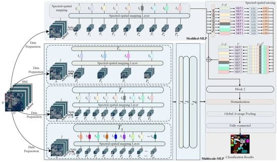
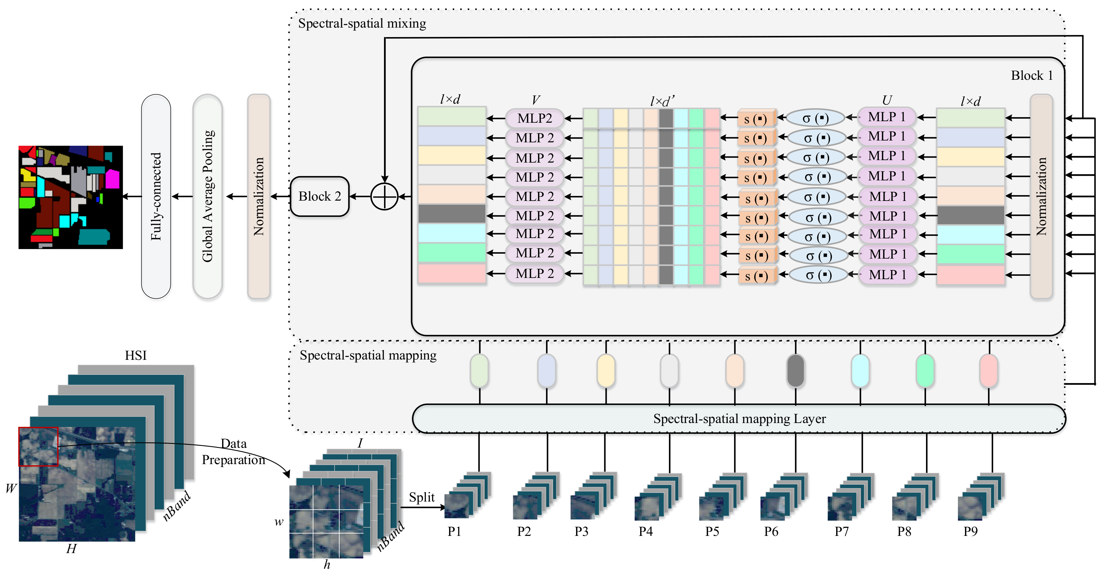
Figure 1 shows the overview architecture of the proposed Modified-MLP for HSI classification. There are three core parts in the Modified-MLP: spectral–spatial feature mapping, spectral–spatial information mixing, and following clssification. We split each input HSI sample into fixed-size 3D patches. Then, each is linearly projected by the spectral–spatial feature mapping layer, resulting in a series of spectral–spatial features. Next, these features are fed into the spectral–spatial information mixing for capturing the spectral–spatial feature interactions of different patches. After that, the classification results are obtained by the fully connected layer. The detailed description is explained as follows.
Suppose the HSI dataset is of size , where and indicate the spatial height and width, respectively, and is the band number. Firstly, a single sample (i.e., ) is generated by processing each pixel in the HSI with a fixed window size, whose shape is .
Secondly, a sample of the HSI is split into patches (i.e., ) without overlapping, , and is calculated as Equation (1). Each patch has a shape of , the size of the clipped patch (i.e., ) is determined empirically. For instance, if the size of a single HSI sample, i.e., , is 3232 (i.e., = 32, = 32), the fixed patch size is set to 4, thus, 64.
Thirdly, all the patches are fed into a spectral–spatial mapping layer independently, here, each patch is linearly projected into an optimal hidden -dimensional spectral–spatial feature space. Here, let represent the output features obtained by the spectral–spatial mapping layer of the Modified-MLP, where is the number of patches and indicates the hidden dimension of the proposed Modified-MLP.
Then, these obtained features are passed through the well-designed Modified-MLP for spectral–spatial information mixing. There are blocks with the same size and structure, and each block is composed of two different MLPs (i.e., MLP1 and MLP2). The number of represents different depth of the model. Figure 1 shows the two blocks (i.e., = 2) as an example. Each block is connected with a layer normalization at the beginning, and every block is followed by the residual connections. Every block can be defined as follows:
where indicates the gaussian error linear unit (GELU) [43] activation function, indicates the weight matrix of MLP 1 with -dimensional output, and refers to the weight matrix of MLP 2. Different from the classical MLP architecture, skip-connections and normalization layer [44] are considered in this study to ensure stable training.
In particular, is the key element to capture the spectral–spatial interactions of different patches in the proposed Modified-MLP, which is built out of basic MLP layers with gating. To capture the crossed spectral–spatial information, it is necessary for to consist of operation over the spectral–spatial dimension. The simplistic option could be described as follows, which is a linear projection:
where , indicates the number of patches, is the bias.
In this study, the crossed information is defined as follows:
where indicates the element-wise multiplication. This operation is inspired by the Gated Linear Units (GLUs) [45], which defines as a spatial depth-wise convolution. Instead of using the convolution operation, we redefine the operation by element-wise multiplicative interaction to capture crossed spectral–spatial information. Similar to the LSTMs, these gates multiply each element of the weight matrix and controls the information passed on. Here, is split into two independent elements formed along the channel dimension to capture the spectral–spatial relationships effectively. The shape of and is the same, which divide the channel dimension of equally. Thus, we set to maintain the value of the input dimension. can be viewed as the gating function, because each value of elements in would be changed according to the by the multiplicative gating. Therefore, the features have strong correction with each other.
Finally, the proposed Modified-MLP applies a normalization layer to alleviate the vanishing problem in the training procedure. At last, average pooling layer and a fully connected layer are used for classifying HSI.
Specifically, the normalization layer is used to normalize the input features, which not only reduces the training time by normalizing neurons, but also alleviates the vanishing or exploding gradient problem [44].
For the average pooling layer, it sums out the spectral–spatial information and takes the average of each feature map. The advantage of the average pooling layer is that there is no parameter to optimize.
The outputs of the average pooling layer are vectorized and fed into fully connected layers and then a softmax layer is used to finish the HSI classification task.
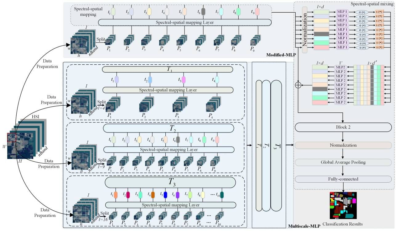
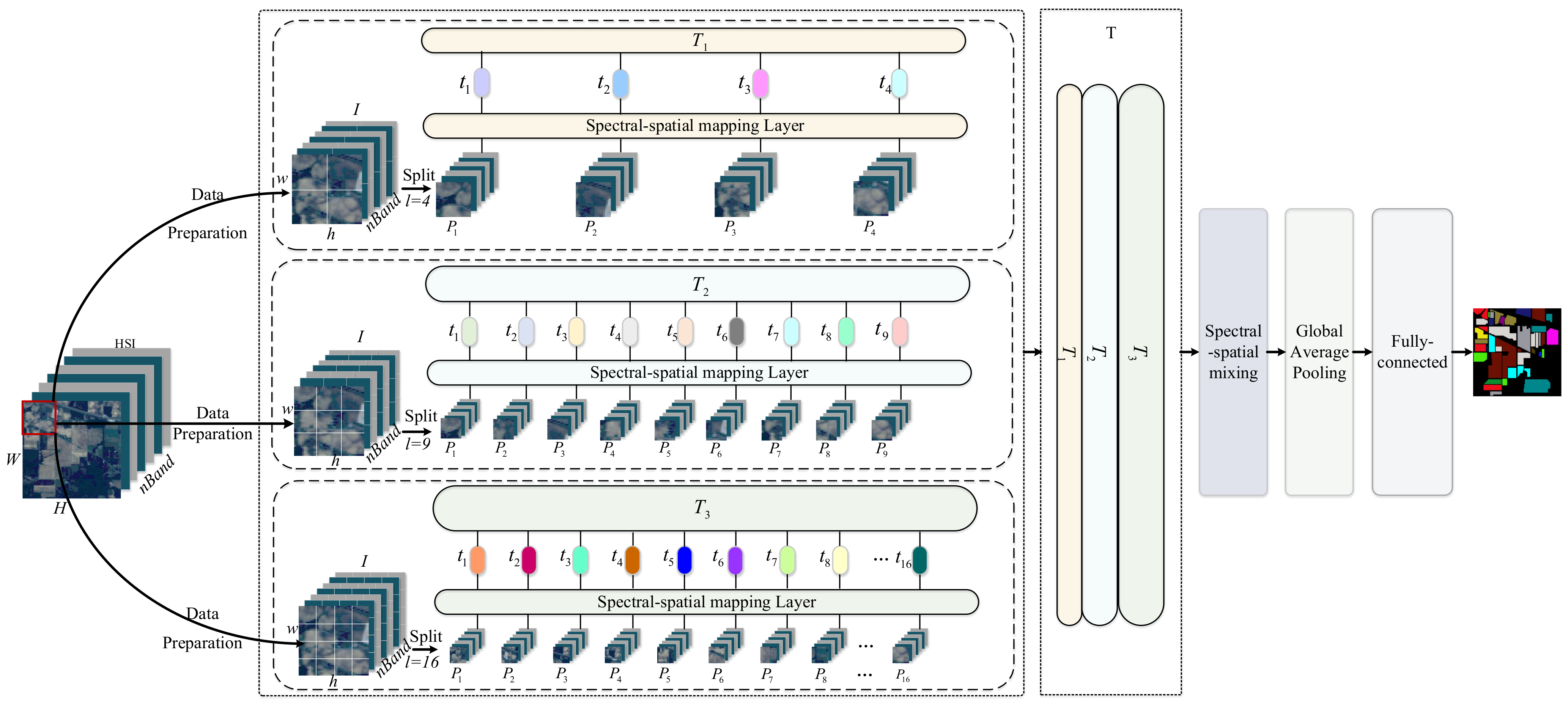
2.2. The Proposed Multiscale-MLP for HSI Classification
The proposed Modified-MLP extracts the spectral–spatial features of each patch independently. However, Modified-MLP uses a fixed scale (i.e., ) to prepare training data. Therefore, Modified-MLP can be enhanced with different scales to fully extract the multiscale spectral–spatial features of HSI inputs. In this section, Multiscale-MLP is proposed, which aims to capture the spectral–spatial information in patches with different scales. Figure 2 shows the framework of the proposed Multiscale-MLP for HSI classification. Specifically, an input HSI sample is divided into fixed-size 3D patches with different patch sizes. Next, each patch is linearly projected by the spectral–spatial feature mapping layer. Then, the obtained features in different scales are fused in different scales so that the patch-level spectral–spatial features can be represented in a multiple scale manner. After that, these features are sent to the spectral–spatial information mixing and the following classification. The detailed steps are explicitly explained as follows.
Firstly, a value of the patch size is set. Thus, there are patches, which can be calculated by Equation (1).
Secondly, a spectral–spatial mapping layer is applied to project each into a fixed dimension.
where is the spectral–spatial mapping operation, refers to the output features of each , and indicates a mapping set with -dimension, whose length and output hidden layer -dimension are both determined by the experiments.
Thirdly, we reset the patch size with different values and repeat the above two steps, hence, there are several with different scales (i.e., = 3, and = 4, 9, and 16) in Figure 2, which is determined by the number of different values of patch sizes. is fused to generate , which can be defined as follows:
Finally, is fed into the spectral–spatial mixing and finish the HSI classification task. The proposed Multiscale-MLP could obtain abundant spectral–spatial information with multiple patches with different sizes.
2.3. The Proposed Soft-MLP for HSI Classification
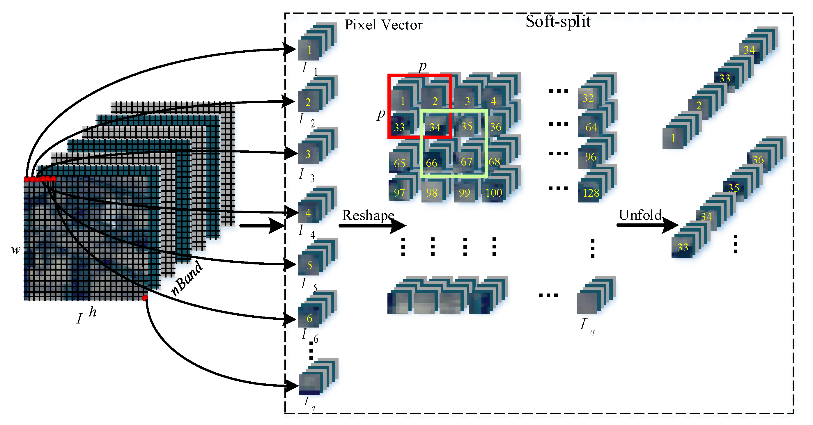
To further improve the HSI classification performance and make full use of different scale information in the network, here, Soft-MLP is proposed with a key part named soft split operation, which not only structurizes the input to patches with variable length, but also fully uses the spectral–spatial information with an overlapping style. Figure 3 displays the detail description of the soft split. Each patch is produced by combining overlapped pixel vectors. Details of the proposed soft split operation are described as follows.
The input HSI sample can be described as , where represents a pixel vector of the given and. Suppose a sample has the shape of 3232, therefore, a single sample contains (i.e., 1024) pixel vectors and all the pixel vectors can be reshaped with any combination.
Next, a patch can be formed by combining different pixel vectors. In Figure 3, four pixel vectors (i.e., 1, 2, 33, and 34) in the input HSI sample are concatenated to form a new patch with size. By applying the soft split, can be calculated as follows:
where is the patch size and and are the spatial height and width of a HSI sample, respectively. refers to the stride (i.e., ) in Figure 3. Since the proposed Soft-MLP splits the input HSI sample into patches with overlapping, each patch is correlated with surrounding patches to establish prior knowledge that there should be stronger correlations between surrounding patches. Thus, the local information can be aggregated from surrounding patches, which is helpful to extract features with multiscale information.
Finally, all the patches are fed into the spectral–spatial mapping layer and spectral–spatial mixing layer to finish HSI classification task, which is similar to the Multiscale-MLP. The proposed Soft-MLP can transform the input HSI sample with different orders and sizes with overlap; therefore, the Soft-MLP helps to make full use of the global relations of different pathes on the input HSI sample.
2.4. The Proposed Soft-MLP-L for HSI Classification
There always exists many learnable parameters in the MLP-based methods with limited samples, which results in an overfitting problem. In order to mitigate this problem, we introduce label smoothing to the proposed MLP-based methods.
For HSI classification, let represent a HSI training sample, and its corresponding label , where indicates the number of classes. Here, can be represented in a one-hot vector with -dimension:
where , indicates the discrete Dirac delta function, and equals 1 for and 0 otherwise.
When we apply label smoothing for HSI classification, is used as the label instead of the original label .
where is a mixture of the original label and the fixed uniform distribution of the number of classes and represents the smoothing factor [46].
3. Experimental Results
3.1. Data Description
The three widely used datasets, including the Salinas, Pavia University (Pavia), and Indian Pines datasets, are used to test the effectiveness of the proposed methods. The detailed information of each dataset is presented as follows.
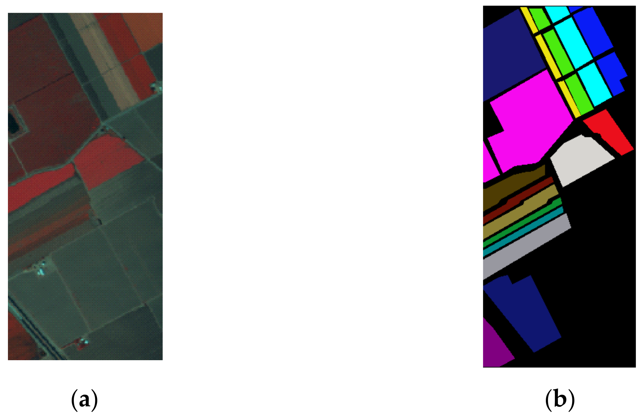
The Salinas dataset was obtained by the Airborne Visible-Infrared Imaging Spectrometer (AVIRIS) sensor over Salinas Valley. This dataset includes 512 × 217 pixels, and its spatial resolution is 3.7 m. The 20 noisy spectral bands have been removed, leading to 204 bands in the range of 0.2–2.4 m. The ground truth consists of 16 classes of interest. Figure 4 displays the false-color composite image and the available ground-truth map. Table 1 gives the number of samples for each class.
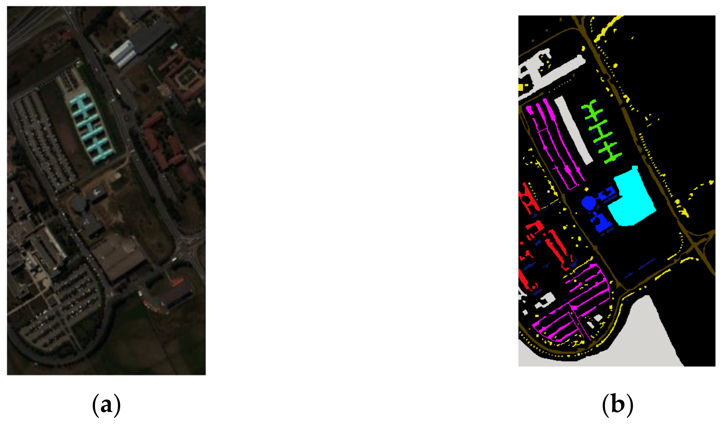
The Pavia dataset was captured by the ROSIS-3 sensor over Pavia University, composed of 103 bands with 610 × 340 pixels after removing the low signal-to-noise ratio (SNR) bands. The spatial resolution of this dataset is 3.7 m, and nine classes were chosen in the ground truth in the experiments. The false-color composite image and the reference map are shown in Figure 5. The samples are reported in Table 2.
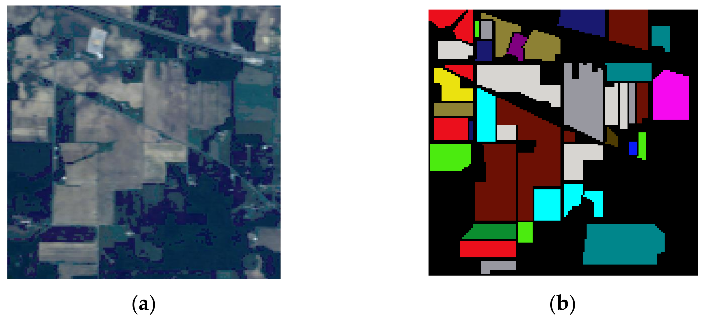
The Indian Pines dataset was acquired by the AVIRIS sensor in 1992. This dataset is 145 × 145 pixels with 103 bands ranging from 0.2–2.4 μm. The water absorption and low signal-to-noise ratio bands (bands 104–108, 150–163, and 220) lead to 200 bands. The ground truth contains 16 land cover types. Figure 6 displays the false-color composite image and the ground truth map. The detailed number of available pixels in each class is reported in Table 3.
3.2. Implementation Details
In the experiments, the dataset is separated into three parts, including the training samples, validation samples, and the test samples. We randomly choose 200 training samples from all the labeled samples, and 50 samples are randomly selected from the remaining as the validation samples; the remaining samples are considered as the test samples. The best model on the validate samples is used to evaluate on the test samples.
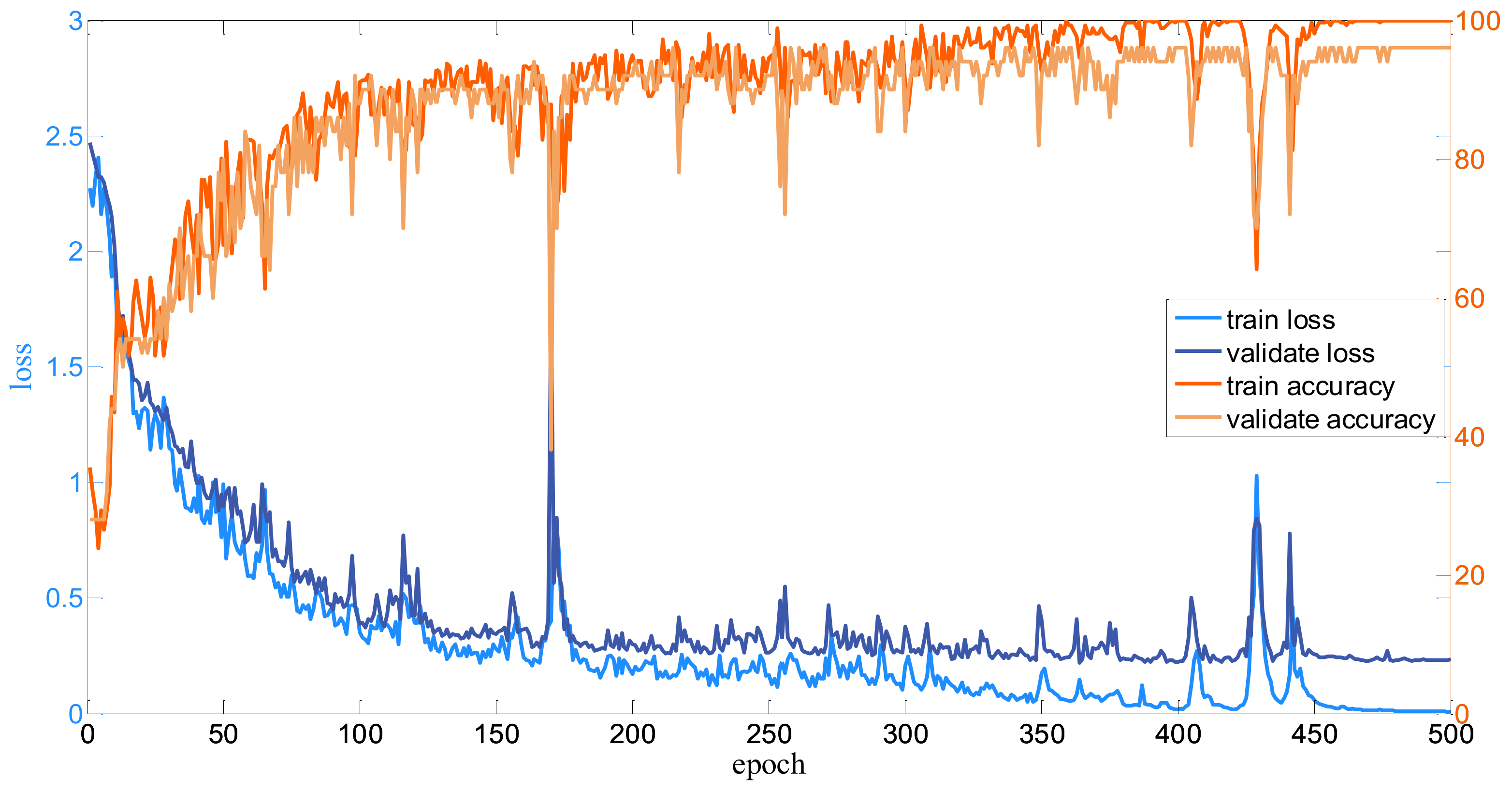
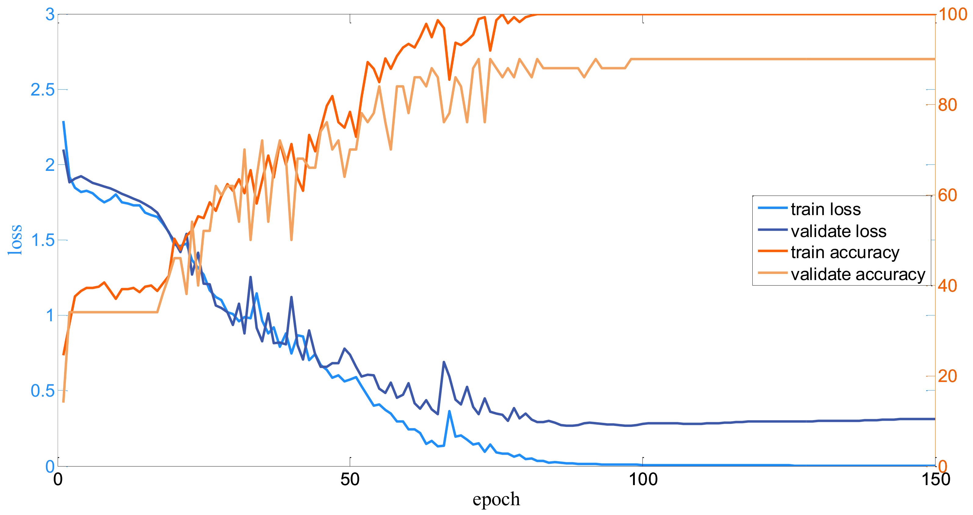
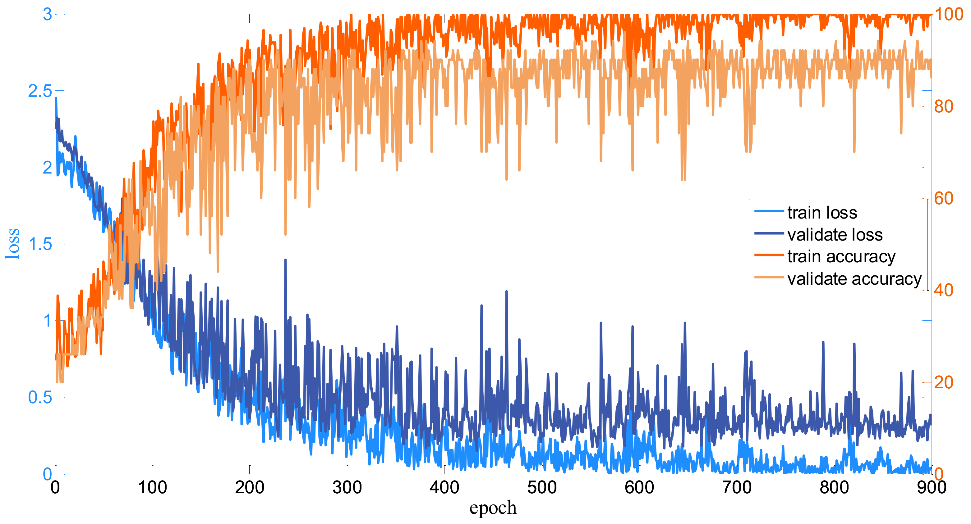
For each dataset, firstly, the input HSI is normalized into [−0.5, 0.5]. Then, the neighbors of each pixel to be classified are set to 3232 as the input of the well-designed model. Since the number of samples are different, the batch size for all the datasets is various. For the Salinas dataset, the bath size is set to 256; for the Pavia dataset, the batch size is set to 128; and for the Indian Pines dataset, the batch size is set to 100. Besides, for the proposed Modified-MLP, the numbers of training epochs are 500, 150, and 900 for the Salinas, Pavia, and Indian Pines datasets, respectively. The number of training epochs is determined by observing the curve of the loss function on the validated samples. To clearly display the training process, take the Modified-MLP as an example. The curves of the proposed Modified-MLP including the loss and accuracy of the training and test for all the datasets are shown in Figure 7, Figure 8 and Figure 9. Thus, the number of epochs is set to 500, 150, and 900 for the Salinas, Pavia, and Indian Pines datasets, respectively, when the learning curve is stable. In addition, for the proposed Multiscale-MLP, Soft-MLP and Soft-MLP-L epochs are both set to 300, 300, and 200 for the Salinas, Pavia, and Indian Pines datasets, respectively. In order to update the training parameters rapidly, the Adam optimizer [47] and decay learning rate are utilized; specifically, initial learning rates are set to 1, 8, and 2 for the Salinas, Pavia, and Indian Pines, respectively. The decay rate every 300 epochs is set to 1/3 for the proposed Modified-MLP. For the Soft-MLP, the learning rate is 8, 8, and 6 for the Salinas, Pavia, and Indian Pines datasets, respectively. To measure the performance of all the methods, overall accuracy (OA), average accuracy (AA), and kappa coefficient (K) are used as the evaluation indexes.
3.3. Parameter Analysis
In order to find the optimal architecture, ablations on scaling different main parameters including the patch sizes, hidden dimensions, and number of blocks are run. The selection of these parameters plays an essential role in model size and the complexity of the proposed Modified-MLP, which should be specially discussed.
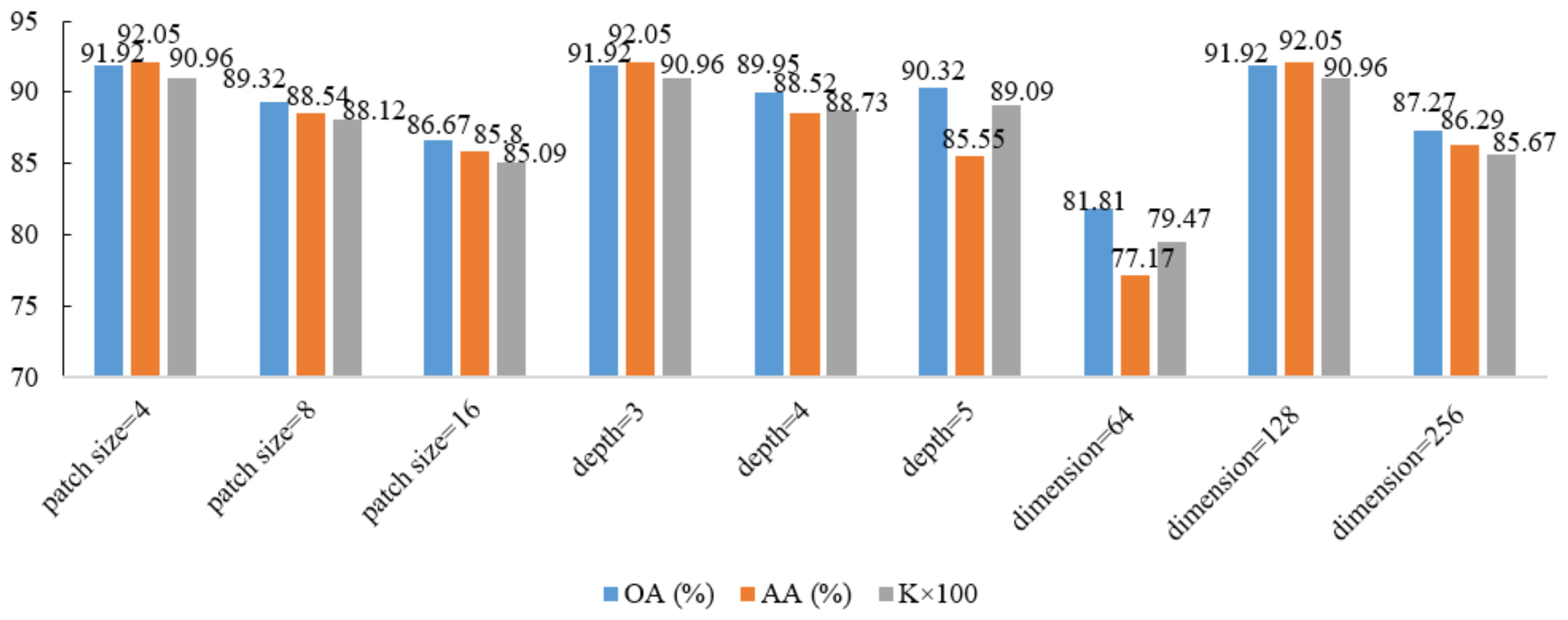
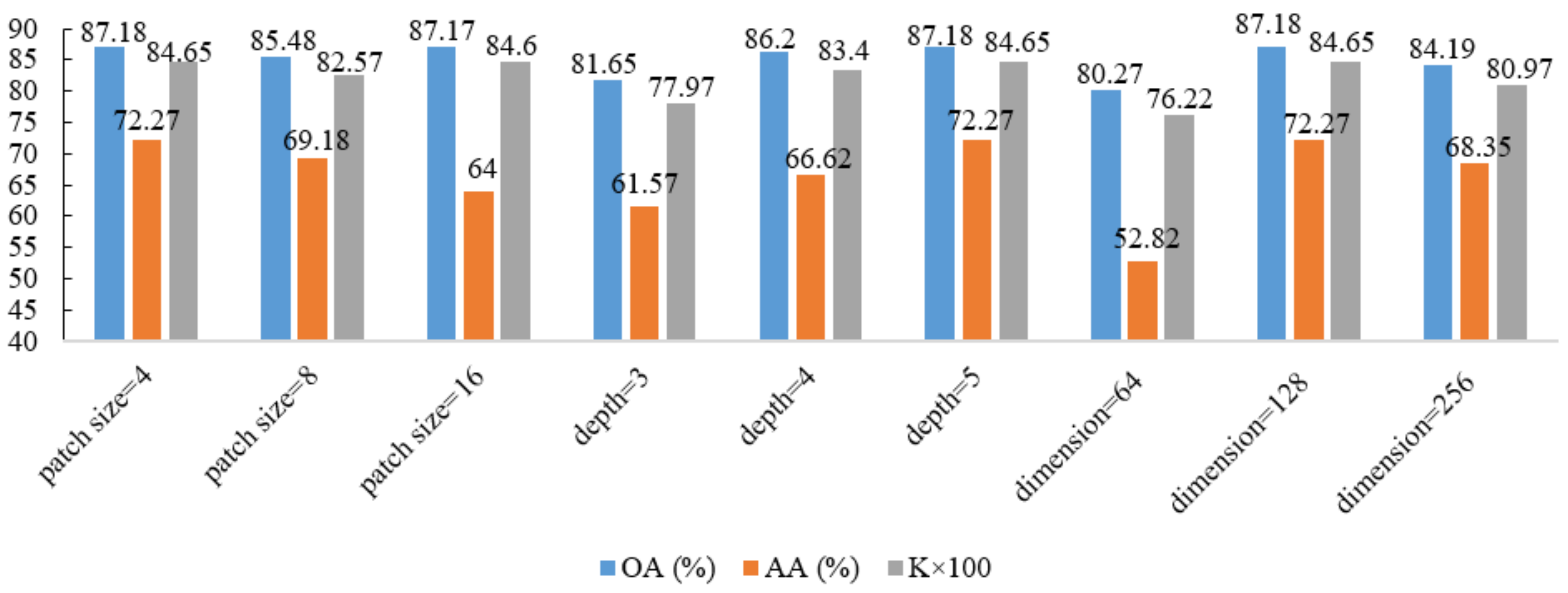
The first parameter is validated on the patch sizes. To capture the relationships of different patches, the input (e.g., 3232) of the proposed Modified-MLP is split into fixed-size patches (e.g., 44, 88, and 1616) for all the datasets, which represent spectral–spatial information at different positions of the input HSI. Meanwhile, the dimensions and number of layers of the proposed Modified-MLP are kept the same. The second parameter is analyzed on the number of blocks of the Modified-MLP, which controls the depth of the model, which we call depth for short. The value of the depth is varied from three to five of the Modified-MLP to find the appropriate value of depth. In addition, the third main parameter is named the dimension of the proposed Modified-MLP. Here, the dimension of the proposed Modified-MLP indicates the hidden dimension in the MLP. With the increment of the model dimension, it is easy for the model to encounter the overfitting problem; thus, different numbers of dimension (i.e., 64, 128, and 256) are chosen to search the optimal value for HSI classification.
The performance of the proposed Modified-MLP of different parameters with 200 training samples is shown in Figure 10, Figure 11 and Figure 12 for the Salinas, Pavia, and Indian Pines datasets, respectively. In the experiments, we use the control variable method for all the datasets. For the case of the model depth, the value of patch size and dimension of the model are fixed, set to 4 and 128, respectively. For the case of patch size, the value of model depth and dimension of the model are also fixed, set to 3 and 128, respectively. Similarly, for the case of dimension of the model, the value of patch size and model depth are fixed, set to 4 and 3, respectively. As shown in Figure 10, Figure 11 and Figure 12, it can be easily seen that for the Salinas and Pavia datasets, with increasing the value of patch size, the accuracies are decreased. In terms of the depth of the proposed Modified-MLP, for the Pavia and Indian Pines datasets, when the value of depth is larger, there are bigger improvements. For the Salinas dataset, when the value of depth is three, Modified-MLP achieves the best classification accuracy. Because there are more bands in the Salinas dataset compared to other datasets, increasing the depth results in more parameters in the MLP, which makes it easier to generate the overfitting problem. In addition, by scaling the width of the hidden layer in the proposed Modified-MLP, Modified-MLP with 128 dimensions reaches the highest OA, AA, and . These results suggest that the proposed Modified-MLP with five layers, dimension = 128, and a patch size of 4 for the Pavia and Indian Pines datasets obtain the highest accuracies, and with three layers, dimension = 128, and a patch size of 4 for the Salinas dataset achieves the best performance.
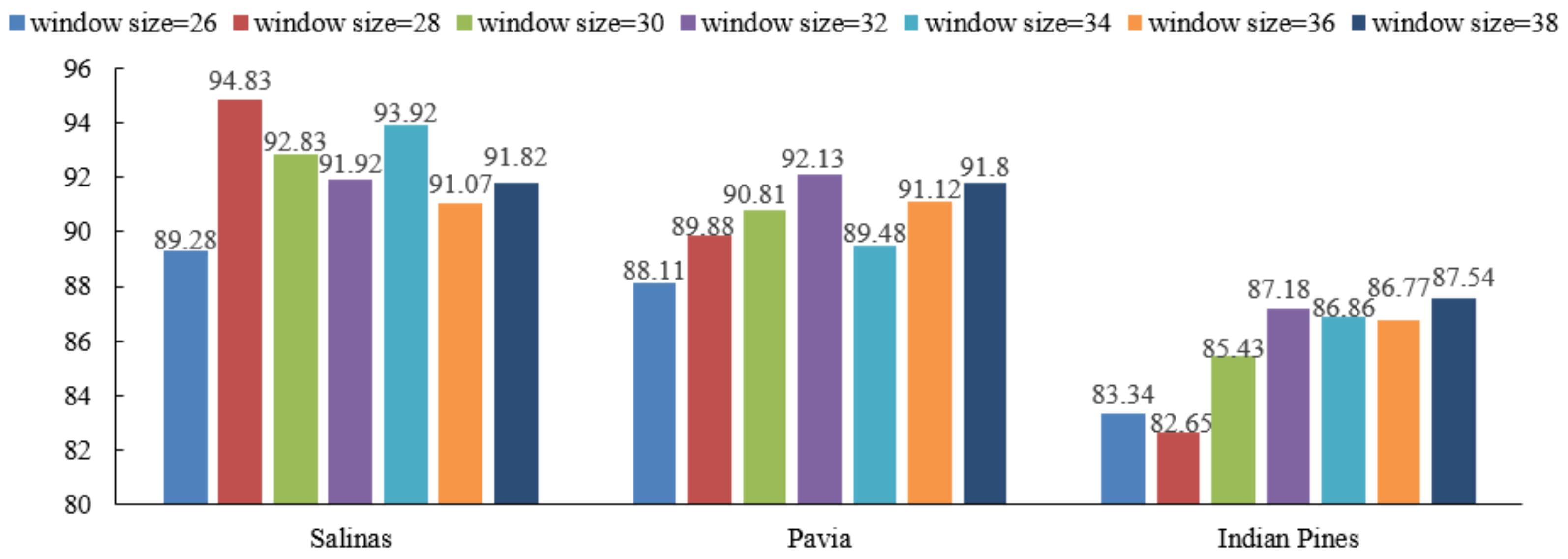
Furthermore, the proposed Multiscale-MLP uses different scales (i.e., scales) to fully extract the multiscale spectral–spatial features with different scales of the HSI inputs. To validate the impact of input size, different spatial window sizes (i.e., 26 × 26, 28 × 28, 30 × 30, 32 × 32, 34 × 34, 36 × 36, and 38 × 38) are used in the experiment, and the results of the proposed Multiscale-MLP on the three datasets are shown in Figure 13.
With different window sizes, there exists a peak. The best spatial window size depends on different datasets. The proposed Multiscale-MLP achieves the best performance concerning the 2828 window size on the Salinas dataset, and the 3232 window size on the Pavia and Indian Pines datasets. If the spatial window size increases, more pixels are used to extract spectral–spatial features; thus, the OA of the proposed Multiscale-MLP increases, too. However, the accuracies begin to decline when the window size reaches a certain value, because more heterogeneous pixels confuse the feature extraction. In the experiments, all the proposed methods are evaluated with 3232 window size to maintain the same setting.
3.4. Comparison of the Proposed Methods with the State-of-the-Art Methods
In the experiments, two classical methods including RBF-SVM [14] and EMP-SVM [48] and four state-of-the-art methods including the CNN [49], SSRN [31], VGG [50], and HybridSN [51] are considered for comparison. For the radial basis function (RBF)-SVM, the optimal value of and are the key parameters, which are searched by the grid searched method in the range of {, ,…, }. In addition, for the extended morphological profiles (EMP)-SVM, in order to extract the spatial information of the HSI, the morphological opening and closing operations are applied. We adopt the disk-shaped structuring element, whose sizes are increasing from two to eight. Then, the generated features are used as the input for the RBF-SVM to finish the final classification task.
The experimental performance of the proposed Modified-MLP, Multiscale-MLP, Soft-MLP, and Soft-MLP-L for hyperspectral classification with 200 training samples are reported in Table 4, Table 5 and Table 6. Compared with the RBF-SVM and EMP-SVM, the proposed Modified-MLP achieves the highest accuracies. For example, compared with the RBF-SVM, the proposed Modified-MLP has superior performance, according to OA, AA, and . Besides, compared to the EMP-SVM, OA, AA, and on the Salinas dataset are increased by 4.33%, 3.4%, and 4.81%, respectively. In addition, compared to the classical methods, the deep learning-based methods generally obtain better performance. The proposed Modified-MLP also has the superiority of the deep learning-based methods. Take the Salinas dataset as an example; compared to the CNN, the OA of the proposed Modified-MLP is increased by 3.52%. Besides, the proposed Modified-MLP exhibits the best OA with the improvement of 3.19% and 2.67% in comparison with the SSRN and VGG, respectively. The classification results on the Pavia and Indian Pines also have the similar situation. All the experimental results reveal the superiority of the proposed Modified-MLP.
Furthermore, different from the proposed Modified-MLP, the proposed Multiscale-MLP achieves 92.25%, 93.50%, and 91.33% in terms of OA, AA, and on the Salinas dataset, respectively. The results demonstrate the superiority of the proposed Multiscale-MLP with multiscale patch sizes. In addition, the proposed Soft-MLP obtains the highest results. For the Salinas dataset, the proposed Soft-MLP is 1.56% and 1.23% higher than Modified-MLP and Multiscale-MLP, respectively. Besides, compared to the classical methods (i.e., RBF-SVM and EMP-SVM) and deep learning-based methods (i.e., CNN, SSRN, VGG, and HybridSN), the proposed Soft-MLP has obvious improvements. Specifically, compared to RBF-SVM and EMP-SVM, the proposed Soft-MLP increases accuracies by 10.39% and 5.89%; 12.96% and 3.59%; 8.62% and 6.84% in terms of OA on the Salinas, Pavia, and Indian Pines, respectively. In addition, for the Indian Pines dataset, compared to the CNN and VGG, the proposed Soft-MLP increases OA by about 2%; for the SSRN and HybridSN, the Soft-MLP has an improvement of nearly 5%. All the results indicate that the proposed Soft-MLP is an effective method. Likewise, the performance of the Pavia and Indian Pines datasets follows the similar trends as the Salinas dataset. The results demonstrate that the proposed Soft-MLP, which applies the soft split operation by separating the input HSI sample into fixed patches with overlapping, is effective.
In addition, the proposed Soft-MLP-L has the best performance of all methods on all datasets. Specifically, the proposed Soft-MLP-L boosts OA by 2.24% for the Salinas dataset, 1.83% for the Pavia dataset, and 2.13% for the Indian Pines dataset, compared to the proposed Modified-MLP with 200 training samples. The proposed Soft-MLP-L also exceeds HybridSN by 3.35%, 2.15%, and 6.23% on the Salinas, Pavia, and Indian Pines datasets, respectively. These results indicate that the proposed MLP-based methods are effective. In the future, we will explore more new ideas in deep learning methods to further improve the classification performance of the MLP-based method.
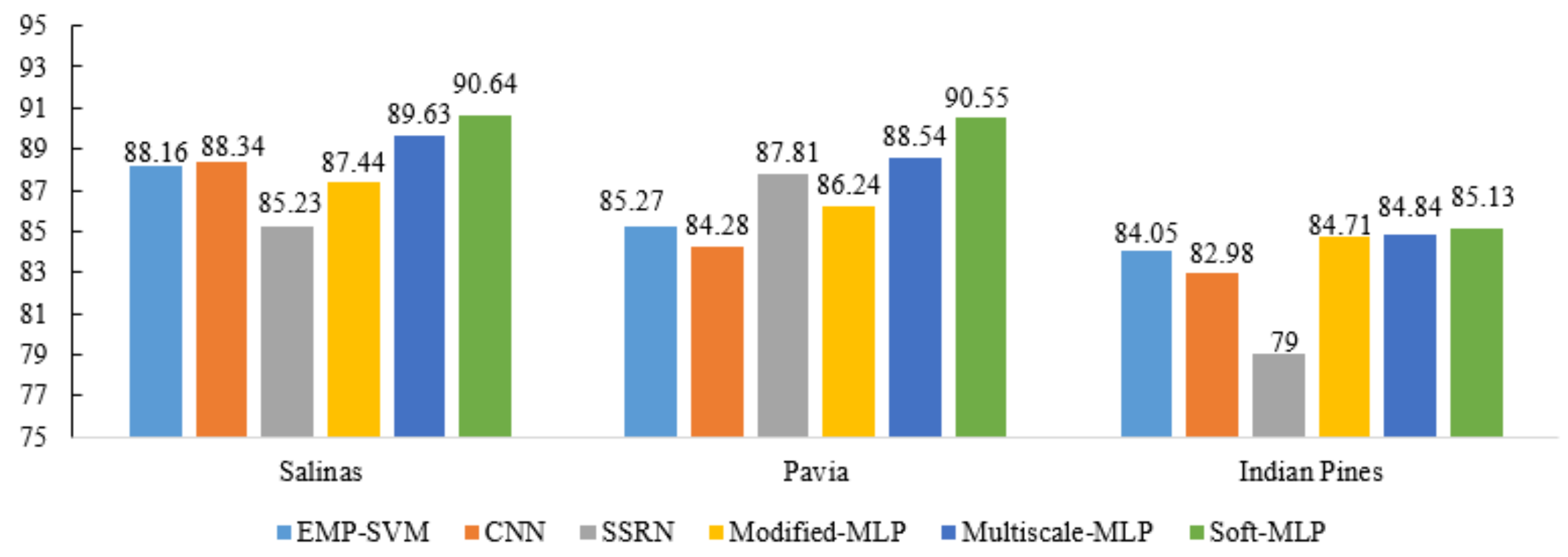
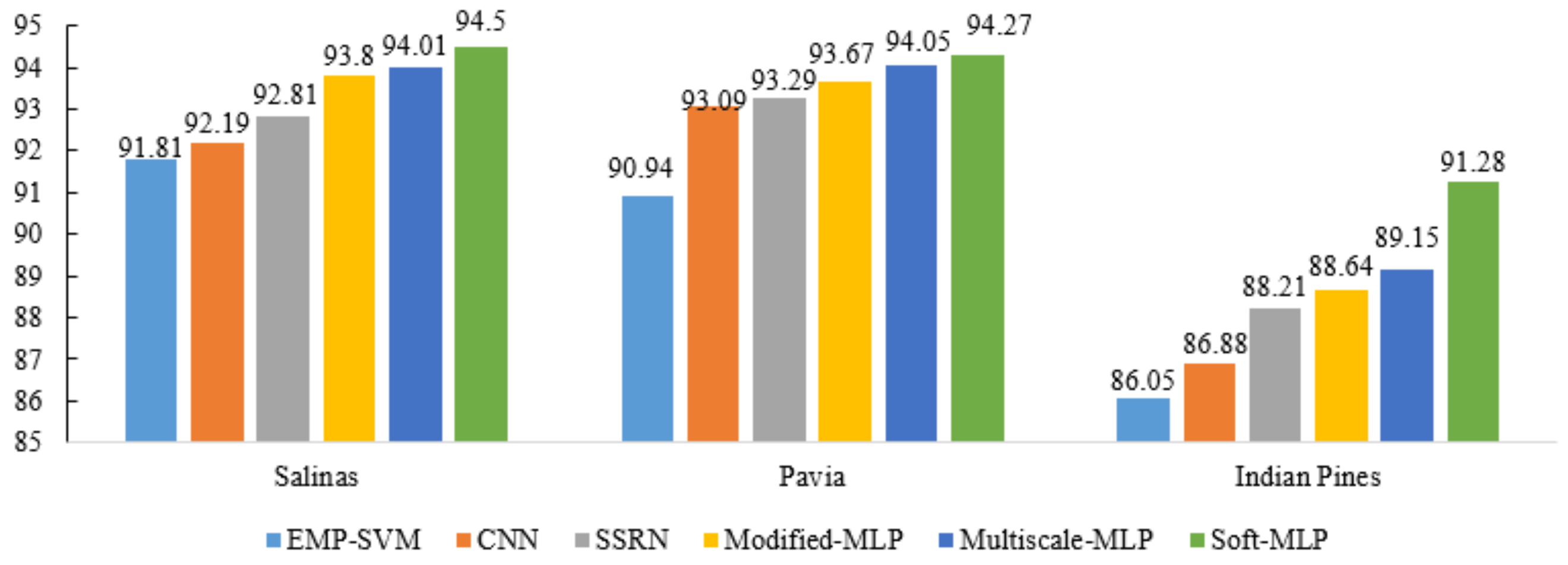
In addition, to validate the proposed methods are effective with different training samples, Figure 14 and Figure 15 show the OA of different methods (i.e., EMP-SVM, CNN, SSRN, Modified-MLP, Multiscale MLP, and Soft-MLP) on the different datasets with 150 and 300 training samples, respectively. Specifically, the proposed Soft-MLP achieves the best performance on the three datasets, which reaches 90.64%, 90.55%, and 85.13% on the Salinas, Pavia, and Indian Pines datasets, respectively, with only 150 training samples. In addition, when 300 training samples are used in the experiments, the proposed MLP-based methods have also achieved better results compared to comparison methods. Especially, for the Indian Pines dataset, the proposed Soft-MLP improves the classification accuracy by 5.23%, 4.4%, and 3.07% compared to EMP-SVM, CNN, and SSRN, respectively. All the results demonstrate that the proposed methods are effective.
3.5. Comparison with Different Methods with Cross-Validation Strategy
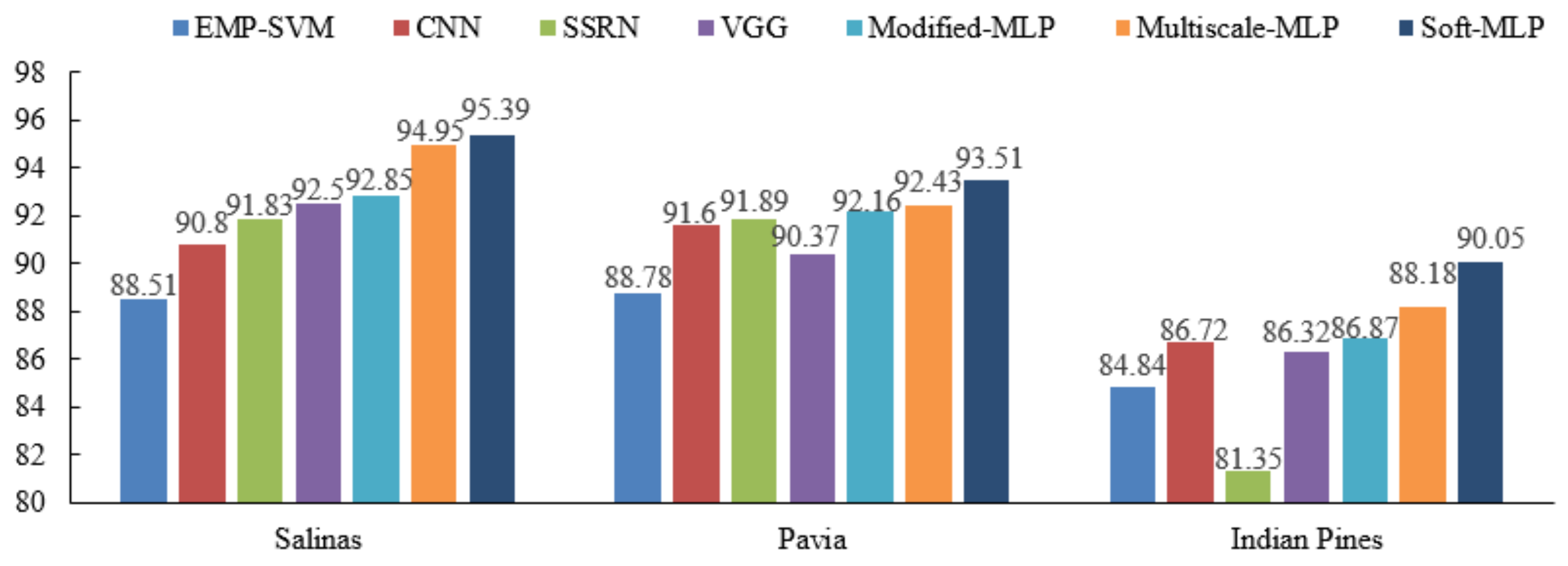
Cross-validation is a popular strategy for model selection, which relies on a preliminary partitioning of the data into subsamples, and each subsample can be selected as the validation sample. In the experiments, the fivefold cross-validation is used with the sum of 200 labeled samples on the three datasets. The results of the corresponding experiments are shown in Figure 16.
One can see that the proposed MLP-based methods also yield the highest OA on the three datasets. Take the Salinas dataset as an example; compared to the other methods (i.e., EMP-SVM, CNN, SSRN, and VGG), the proposed Soft-MLP improves the OA by 6.88%, 4.59%, 3.56%, and 2.89%, respectively. The results demonstrate that the proposed methods (i.e., Modified-MLP, Multiscale-MLP, and Soft-MLP) have better performance compared with other comparison methods.
3.6. Comparison the Running Time and Computational Complexity of the Proposed Methods with the State-of-the-Art Methods
In order to comprehensively analyze the proposed approaches and the state-of-the-art methods, here, computational cost of different methods is analyzed, which is reported in Table 7. All the experiments are conducted on a computer with an Intel Xeon Silver 4210R processor with 2.4 GHz, 128GB of DDR4 RAM, and an NVIDIA Tesla V100 graphical processing unit (GPU). From the view of the running time, the proposed Soft-MLP consumes more time compared to other deep learning-based methods on all the datasets, due to each input of the model being split into several fixed patches with overlapping. Thus, the number of the patches is larger than other methods, which adds the dimension of the input of the proposed Soft-MLP. For the proposed Modified-MLP method, compared to the SSRN, the training time is shorter. Take the Salinas dataset as an example; due to the fact that the number of epochs of Modified-MLP is smaller than SSRN, the training time reduces by 77.55 s. Compared to CNN and VGG, the training time of Modified-MLP takes longer on the three datasets. In addition, compared to the Modified-MLP, the training time and test time of the proposed Soft-MLP and Soft-MLP-L are longer, but these methods obtain better classification performance.
In addition, the number of floating-point operations (FLOPs) [52] of different methods is also reported in Table 7. Compared to the VGG and SSRN, the proposed Modified-MLP has smaller FLOPs on the Salinas dataset. The proposed Modified-MLP needs fewer FLOPs compared to the VGG on the Pavia and Indian Pines datasets. Besides, the number of parameters of various approaches is also computed, which is shown in the last column in Table 7. From the results, compared to the VGG, there are fewer parameters in the proposed Modified-MLP, Multiscale-MLP, Soft-MLP, and Soft-MLP-L on all the datasets. Compared to the CNN and SSRN, the proposed methods have more total parameters because the depth and width of the proposed methods are larger, which results in increasing FLOPs and total parameters, but the accuracies of the proposed methods are the highest. Specifically, compared to the Modified-MLP, Multiscale-MLP increases the FLOPs by 75.89 Mbytes, 43.12 Mbytes, and 62.26 Mbytes, and increases the total parameters by 8.45 Mbytes, 4.32 Mbytes, and 7.98 Mbytes on the Salinas, Pavia, and Indian Pines datasets, respectively. Because the proposed Multiscale-MLP aims to capture the spectral–spatial information in patches with different scales and the proposed Soft-MLP transforms the input HSI sample with an overlap style, there are larger FLOPs and total parameters compared to the proposed Modified-MLP. For the proposed Soft-MLP-L, it is similar to the Soft-MLP in terms of FLOPs and total parameters on the three datasets, which demonstrates that Soft-MLP-L is an effective method for HSI classification.
3.7. Classification Maps
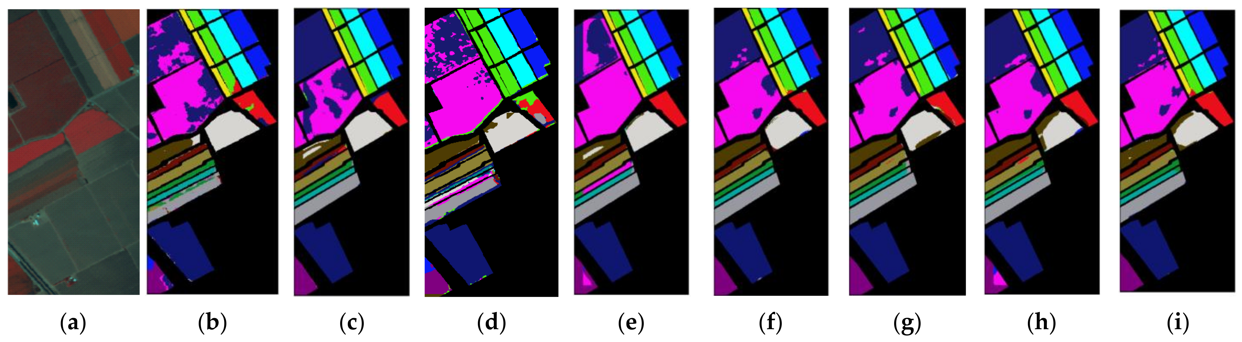
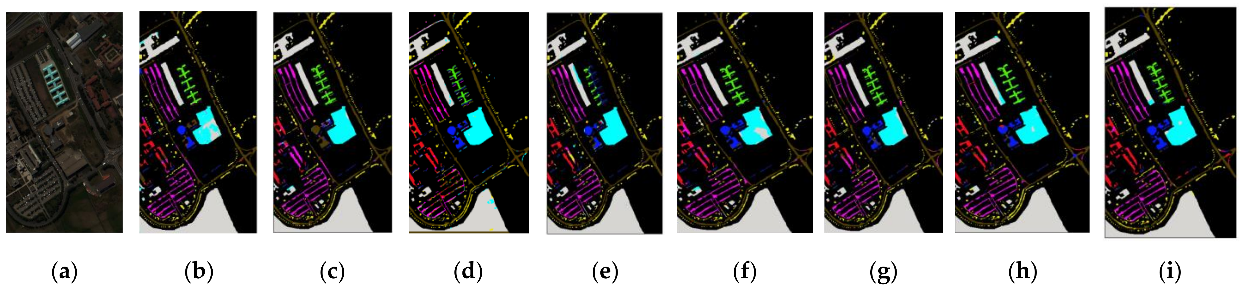
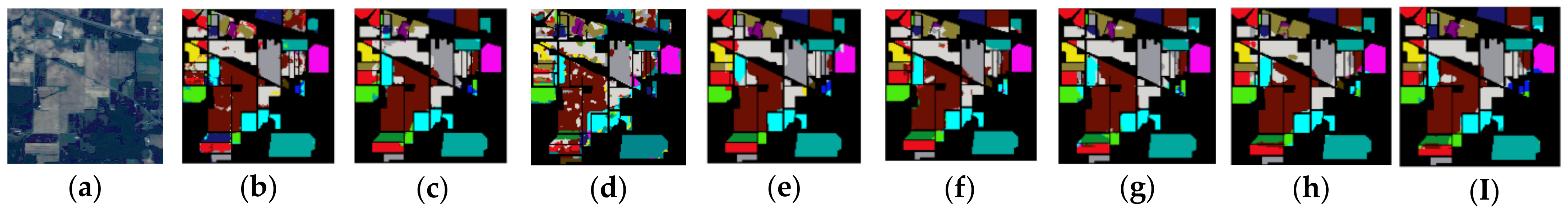
To facilitate visual comparison, the classification maps of different approaches for all the datasets with 200 training samples are displayed in Figure 17, Figure 18 and Figure 19. As can be seen from these figures, compared to the classical method EMP-SVM and deep learning-based methods including CNN, SSRN, VGG, our proposed methods have more precise classification results. More specifically, there are noisier scatter points in the classification map of EMP-SVM compared to deep learning-based methods on the three datasets. Take the Pavia dataset as an example; for the class of Bitumen color in blue shown in Figure 17b–i, the proposed Modified-MLP appears to be more smoothing. Furthermore, metal sheets color in green depicts more errors compared to the proposed Modified-MLP, Multiscale-MLP, and Soft-MLP. All the figures reveal that the proposed methods (i.e., Modified-MLP, Multiscale-MLP, Soft-MLP, and Soft-MLP-L) stand out from other competitors.
3.8. Experimental Summary
Overall, compared to the traditional methods (i.e., RBF-SVM and EMP-SVM) and deep learning-based approaches (i.e., CNN, VGG, SSRN, and HybridSN), the overall accuracies of all the proposed methods (i.e., Modified-MLP, Multiscale-MLP, Soft-MLP, and Soft-MLP-L) have improvements on the three public HSI datasets and the corresponding classification maps have also demonstrated that the proposed methods achieve competitive performance. In addition, the total parameters, FLOPs, and time of the proposed methods are larger compared to other methods, but the accuracies of the proposed methods are the highest. To some extent, the proposed methods based on the well-designed MLPs have potential for HSI classification.
4. Conclusions
This study presented modified MLP-based methods for HSI classification, which demonstrated that the proposed MLPs obtained good classification performance compared with state-of-the-art CNNs.
Specifically, compared to the traditional MLP architecture, the Modified-MLP was composed of the spectral–spatial feature mapping and spectral–spatial information mixing with a new architecture (i.e., normalization layer, residual connections, and GELU operations). Modified-MLP learned long-range spectral–spatial feature interactions in and among different patches, which were useful for HSI classification. Moreover, the Multiscale-MLP was exploited to capture adaptive spectral–spatial information with multiple scales, which was conveyed by patch-level input sufficiently. Furthermore, another Soft-MLP was investigated to enhance classification results flexibly by applying soft split operation, which was able to change the fixed-size patch into variable size with overlapping at any length; therefore, each patch is correlated with its surrounding patches. Compared to the popular spectral–spatial extraction methods, the proposed MLP-based approaches (i.e., Modified-MLP, Multiscale-MLP, and Soft-MLP) led to better results with limited training samples. This study demonstrates that the solely MLP-based HSI classification methods have obtained impressive results without convolution operation. Most of all, this study opens a new window for further research of HSI classification, which demonstrates that the well-designed MLPs can also obtain remarkable classification performance of HSI.
Although it is an early try of MLP-based HSI classification, the modified MLPs obtained better classification performance compared to traditional methods (i.e., RBF-SVM and EMP-SVM) and many recently proposed deep learning-based methods such as CNN, SSRN, VGG, and HybridSN.
Recently, much progress has been achieved in the machine learning community and some of them, such as transfer learning, can be combined with MLP to further improve the performance of MLP-based HSI classification.
Author Contributions
Conceptualization: Y.C.; methodology: X.H. and Y.C.; writing—original draft preparation: X.H. and Y.C. Both authors have read and agreed to the published version of the manuscript.
Funding
This research was funded by the Natural Science Foundation of China under the Grant 61971164.
Data Availability Statement
Publicly available datasets were analyzed in this study. This data can be found here: http://www.ehu.eus/ccwintco/index.php?title=Hyperspectral_Remote_Sensing_Scenes accessed on 15 July 2018.
Conflicts of Interest
The authors declare no conflict of interest.
References
- Rußwurm, M.; Körner, M. Temporal vegetation modelling using long short-term memory networks for crop identification from medium-resolution multi-spectral satellite images. In Proceedings of the 2017 IEEE Conference on Computer Vision and Pattern Recognition Workshops (CVPRW), Honolulu, HI, USA, 21–26 July 2017; pp. 1496–1504. [Google Scholar]
- El-Magd, I.A.; El-Zeiny, A. Quantitative hyperspectral analysis for characterization of the coastal water from Damietta to Port Said, Egypt. Egypt. J. Remote Sens. Space Sci. 2014, 17, 61–76. [Google Scholar] [CrossRef] [Green Version]
- Tang, Y.; Chen, M.; Wang, C.; Luo, L.; Li, J.; Lian, G.; Zou, X. Recognition and localization methods for vision-based fruit picking robots: A review. Front. Plant Sci. 2020, 11, 510. [Google Scholar] [CrossRef]
- Hestir, E.; Brando, V.; Bresciani, M.; Giardino, C.; Matta, E.; Villa, P.; Dekker, A. Measuring freshwater aquatic ecosystems: The need for a hyperspectral global mapping satellite mission. Remote Sens. Environ. 2015, 167, 181–195. [Google Scholar] [CrossRef] [Green Version]
- Han, Y.; Li, J.; Zhang, Y.; Hong, Z.; Wang, J. Sea ice detection based on an improved similarity measurement method using hyperspectral data. Sensors 2017, 17, 1124. [Google Scholar] [CrossRef] [Green Version]
- Shang, X.; Chisholm, L. Classification of Australian native forest species using hyperspectral remote sensing and ma-chine-learning classification algorithms. IEEE J. Sel. Topics Appl. Earth Observ. Remote Sens. 2014, 7, 2481–2489. [Google Scholar] [CrossRef]
- Peerbhay, K.; Mutanga, O.; Ismail, R. Random Forests Unsupervised Classification: The Detection and Mapping of Solanum mauritianum Infestations in Plantation Forestry Using Hyperspectral Data. IEEE J. Sel. Top. Appl. Earth Obs. Remote Sens. 2015, 8, 3107–3122. [Google Scholar] [CrossRef]
- Shimoni, M.; Haelterman, R.; Perneel, C. Hypersectral imaging for military and security applications: Combining myriad processing and sensing techniques. IEEE Geosci. Remote Sens. Mag. 2019, 7, 101–117. [Google Scholar] [CrossRef]
- Chen, M.; Tang, Y.; Zou, X.; Huang, Z.; Zhou, H.; Chen, S. 3D global mapping of large-scale unstructured orchard integrating eye-in-hand stereo vision and SLAM. Comput. Electron. Agric. 2021, 187, 106237. [Google Scholar] [CrossRef]
- Chen, M.; Tang, Y.; Zou, X.; Huang, K.; Li, L.; He, Y. High-accuracy multi-camera reconstruction enhanced by adaptive point cloud correction algorithm. Opt. Lasers Eng. 2019, 122, 170–183. [Google Scholar] [CrossRef]
- Audebert, N.; Le Saux, B.; Lefevre, S. Deep Learning for Classification of Hyperspectral Data: A Comparative Review. IEEE Geosci. Remote Sens. Mag. 2019, 7, 159–173. [Google Scholar] [CrossRef] [Green Version]
- Rasti, B.; Hong, D.; Hang, R.; Ghamisi, P.; Kang, X.; Chanussot, J.; Benediktsson, J.A. Feature Extraction for Hyperspectral Imagery: The Evolution From Shallow to Deep: Overview and Toolbox. IEEE Geosci. Remote Sens. Mag. 2020, 8, 60–88. [Google Scholar] [CrossRef]
- Fauvel, M.; Benediktsson, J.A.; Chanussot, J.; Sveinsson, J.R. Spectral and Spatial Classification of Hyperspectral Data Using SVMs and Morphological Profiles. IEEE Trans. Geosci. Remote Sens. 2008, 46, 3804–3814. [Google Scholar] [CrossRef] [Green Version]
- Benediktsson, J.A.; Palmason, J.; Sveinsson, J.R. Classification of hyperspectral data from urban areas based on extended morphological profiles. IEEE Trans. Geosci. Remote Sens. 2005, 43, 480–491. [Google Scholar] [CrossRef]
- Mura, M.D.; Villa, A.; Benediktsson, J.A.; Chanussot, J.; Bruzzone, L. Classification of Hyperspectral Images by Using Extended Morphological Attribute Profiles and Independent Component Analysis. IEEE Geosci. Remote Sens. Lett. 2011, 8, 542–546. [Google Scholar] [CrossRef] [Green Version]
- Fang, L.; He, N.; Li, S.; Ghamisi, P.; Benediktsson, J.A. Extinction Profiles Fusion for Hyperspectral Images Classification. IEEE Trans. Geosci. Remote Sens. 2018, 56, 1803–1815. [Google Scholar] [CrossRef]
- Gualtieri, J.A.; Cromp, R.F. Support vector machines for hyperspectral remote sensing classification. In Proceedings of the Inter-National Society for Optical Engineering, Santa Clara, CA, USA, 8–10 February 1999; Volume 3584, pp. 221–232. [Google Scholar] [CrossRef] [Green Version]
- Chen, Y.; Lin, Z.; Zhao, X.; Wang, G.; Gu, Y. Deep Learning-Based Classification of Hyperspectral Data. IEEE J. Sel. Top. Appl. Earth Obs. Remote Sens. 2014, 7, 2094–2107. [Google Scholar] [CrossRef]
- Zhong, P.; Gong, Z.; Li, S.; Schönlieb, C.-B. Learning to diversify deep belief networks for hyperspectral image classification. IEEE Trans. Geosci. Remote Sens. 2017, 55, 3516–3530. [Google Scholar] [CrossRef]
- Mou, L.; Ghamisi, P.; Zhu, X.X. Deep recurrent neural networks for hyperspectral image classification. IEEE Trans. Geosci. Remote Sens. 2017, 55, 3639–3655. [Google Scholar] [CrossRef] [Green Version]
- Chen, Y.; Jiang, H.; Li, C.; Jia, X.; Ghamisi, P. Deep Feature Extraction and Classification of Hyperspectral Images Based on Convolutional Neural Networks. IEEE Trans. Geosci. Remote Sens. 2016, 54, 6232–6251. [Google Scholar] [CrossRef] [Green Version]
- He, N.; Paoletti, M.; Haut, J.; Fang, L.; Li, S.; Plaza, A.; Plaza, J. Feature extraction with multiscale covariance maps for hyperspectral image classification. IEEE Trans. Geosci. Remote Sens. 2019, 57, 202–216. [Google Scholar] [CrossRef]
- Hu, W.; Huang, Y.; Wei, L.; Zhang, F.; Li, H.-C. Deep convolutional neural networks for hyperspectral image classification. J. Sens. 2015, 2015, 1–12. [Google Scholar] [CrossRef] [Green Version]
- Li, W.; Wu, G.; Zhang, F.; Du, Q. Hyperspectral image classification using deep pixel-pair features. IEEE Trans. Geosci. Remote Sens. 2016, 55, 844–853. [Google Scholar] [CrossRef]
- Kang, X.; Zhuo, B.; Duan, P. Dual-path network-based hyperspectral image classification. IEEE Geosci. Remote Sens. Lett. 2019, 16, 447–451. [Google Scholar] [CrossRef]
- Haut, J.M.; Paoletti, M.E.; Plaza, J.; Plaza, A.; Li, J. Visual Attention-Driven Hyperspectral Image Classification. IEEE Trans. Geosci. Remote Sens. 2019, 57, 8065–8080. [Google Scholar] [CrossRef]
- Ghamisi, P.; Plaza, J.; Chen, Y.; Li, J.; Plaza, A.J. Advanced spectral classifiers for hyperspectral images: A review. IEEE Geosci. Remote Sens. Mag. 2017, 5, 8–32. [Google Scholar] [CrossRef] [Green Version]
- Ma, W.; Yang, Q.; Wu, Y.; Zhao, W.; Zhang, X. Double-branch multi-attention mechanism network for hyperspectral image classification. Remote Sens. 2019, 11, 1307. [Google Scholar] [CrossRef] [Green Version]
- Li, R.; Zheng, S.; Duan, C.; Yang, Y.; Wang, X. Classification of Hyperspectral Image Based on Double-Branch Dual-Attention Mechanism Network. Remote Sens. 2020, 12, 582. [Google Scholar] [CrossRef] [Green Version]
- Alam, F.; Zhou, J.; Liew, A.; Jia, X.; Chanussot, J.; Gao, Y. Conditional random field and deep feature learning for hyper-spectral image classification. IEEE Trans. Geosci. Remote Sens. 2019, 57, 8065–8080. [Google Scholar] [CrossRef] [Green Version]
- Zhong, Z.; Li, J.; Luo, Z.; Chapman, M. Spectral-spatial residual network for hyperspectral image classification: A 3-D deep learning framework. IEEE Trans. Geosci. Remote Sens. 2018, 56, 847–858. [Google Scholar] [CrossRef]
- Song, M.; Shang, X.; Chang, C.-I. 3-D receiver operating characteristic analysis for hyperspectral image classification. IEEE Trans. Geosci. Remote Sens. 2020, 58, 8093–8115. [Google Scholar] [CrossRef]
- Tang, X.; Meng, F.; Zhang, X.; Cheung, Y.-M.; Ma, J.; Liu, F.; Jiao, L. Hyperspectral image classification based on 3-D octave convolution with spatial-spectral attention network. IEEE Trans. Geosci. Remote Sens. 2021, 59, 2430–2447. [Google Scholar] [CrossRef]
- Li, Y.; Zhang, H.; Shen, Q. Spectral-spatial classification of hyperspectral imagery with 3D convolutional neural network. Remote Sens. 2017, 9, 67. [Google Scholar] [CrossRef] [Green Version]
- Li, S.; Song, W.; Fang, L.; Chen, Y.; Ghamisi, P.; Benediktsson, J.A. Deep learning for hyperspectral image classification: An overview. IEEE Trans. Geosci. Remote Sens. 2019, 57, 6690–6709. [Google Scholar] [CrossRef] [Green Version]
- Lu, W.; Wang, X. Overview of hyperspectral image classification. J. Sens. 2020, 2020, 4817234. [Google Scholar]
- Oquab, M.; Bottou, L.; Laptev, I.; Sivic, J. Learning and transferring mid-level image representations using convolutional neural networks. In Proceedings of the 2014 IEEE Conference on Computer Vision and Pattern Recognition, Columbus, OH, USA, 23–28 June 2014; pp. 1717–1724. [Google Scholar] [CrossRef] [Green Version]
- Tang, G.; Mathias, M.; Rio, A.; Sennrich, R. Why self-attention? A targeted evaluation of neural machine translation architectures. arXiv 2018, arXiv:1808.08946v3. Available online: https://arxiv.org/pdf/1808.08946v3.pdf (accessed on 11 November 2020).
- Rumelhart, D.E.; Hinton, G.E.; Williams, R.J. Learning internal representations by error propagation. In Readings in Cognitive Science; Elsevier: Amsterdam, The Netherlands, 1985. [Google Scholar] [CrossRef]
- Thakur, A.; Mishra, D. Hyper spectral image classification using multilayer perceptron neural network & functional link ANN. In Proceedings of the 2017 7th International Conference on Cloud Computing, Data Science & Engineering—Confluence, Noida, India, 12–13 January 2017; pp. 639–642. [Google Scholar] [CrossRef]
- Garcia, B.; Ponomaryov, V.; Robles, M. Parallel multilayer perceptron neural network used for hyperspectral image classification. In Proceedings of the Real-Time Image and Video Processing 2016 International Society for Optics and Photonics, Boulder, CO, USA, 25–28 September 2016; pp. 1–14. [Google Scholar]
- Kalaiarasi, G.; Maheswari, S. Frost filtered scale-invariant feature extraction and multilayer perceptron for hyperspectral image classification. arXiv 2020, arXiv:2006.12556. Available online: https://arxiv.org/ftp/arxiv/papers/2006/2006.12556.pdf (accessed on 2 November 2012).
- Hendrycks, D.; Gimpel, K. Gaussian error linear units (GELUs). arXiv 2020, arXiv:1606.08415. Available online: https://arxiv.org/pdf/1606.08415.pdf (accessed on 8 July 2020).
- Ba, J.; Kiros, J.; Hinton, G. Layer normalization. arXiv 2016, arXiv:1607.06450. Available online: https://arxiv.org/pdf/1607.06450v1.pdf (accessed on 21 July 2016).
- Dauphin, Y.; Fan, A.; Auli, M.; Grangier, D. Language modeling with gated convolutional networks. In Proceedings of the International Conference on Machine Learning, Sydney, Australia, 6–11 August 2017; pp. 10–19. [Google Scholar]
- Muller, R.; Kornblith, S.; Hinton, G. When does label smoothing help? In Proceedings of the NeurIPS, Vancouver, BC, Canada, 8–14 December 2019; pp. 4696–4705. [Google Scholar]
- Aurelio, Y.S.; Almeida, G.; De Castro, C.L.; Braga, A.P. Learning from imbalanced data sets with weighted cross-entropy function. Neural Process. Lett. 2019, 50, 1937–1949. [Google Scholar] [CrossRef]
- Melgani, F.; Lorenzo, B. Classification of hyperspectral remote sensing images with support vector machines. IEEE Trans. Geosci. Remote Sens. 2004, 42, 1778–1790. [Google Scholar] [CrossRef] [Green Version]
- Chen, Y.; Zhu, L.; Ghamisi, P.; Jia, X.; Li, G.; Tang, L. Hyperspectral Images Classification With Gabor Filtering and Convolutional Neural Network. IEEE Geosci. Remote Sens. Lett. 2017, 14, 2355–2359. [Google Scholar] [CrossRef]
- Simonyan, K.; Zisserman, A. Very deep convolutional networks for large-scale image recognition. In Proceedings of the Interna-tional Conference on Learning Representations, San Diego, CA, USA, 7–9 May 2015; pp. 1–14. [Google Scholar]
- Roy, S.K.; Krishna, G.; Dubey, S.R.; Chaudhuri, B.B. HybridSN: Exploring 3-D–2-D CNN Feature Hierarchy for Hyperspectral Image Classification. IEEE Geosci. Remote Sens. Lett. 2020, 17, 277–281. [Google Scholar] [CrossRef] [Green Version]
- Molchanov, P.; Tyree, S.; Karras, T.; Aila, T.; Kautz, J. Pruning convolutional neural networks for resource efficient inference. arXiv 2017, arXiv:1611.06440. Available online: https://arxiv.org/pdf/1611.06440.pdf (accessed on 8 June 2017).
Figure 1.
The overview architecture of the proposed Modified-MLP for HSI classification.

Figure 2.
The framework of the proposed Multiscale-MLP for HSI classification.

Figure 3.
An example of the soft split operation in the Soft-MLP.

Figure 4.
The Salinas dataset. (a) False-color composite image; (b) ground truth map.

Figure 5.
The Pavia University dataset. (a) False-color composite image; (b) ground truth map.

Figure 6.
The Indian Pines dataset. (a) False-color composite image; (b) ground truth map.

Figure 7.
Curves on the Salinas dataset.

Figure 8.
Curves on the Pavia dataset.

Figure 9.
Curves on the Indian Pines dataset.

Figure 10.
Test accuracy of key parameters on the Salinas dataset.

Figure 11.
Test accuracy of key parameters on the Pavia dataset.

Figure 12.
Test accuracy of key parameters on the Indian dataset.

Figure 13.
Results of Multiscale-MLP with different window sizes.

Figure 14.
Test accuracy (%) comparisons under different methods on the three datasets with 150 training samples.
Figure 14.
Test accuracy (%) comparisons under different methods on the three datasets with 150 training samples.

Figure 15.
Test accuracy (%) comparisons under different methods on the three datasets with 300 training samples.
Figure 15.
Test accuracy (%) comparisons under different methods on the three datasets with 300 training samples.

Figure 16.
Results of different methods with cross-validation.

Figure 17.
Salinas. (a) False-color composite image. The classification maps using (b) EMP-SVM; (c) CNN; (d) SSRN; (e) VGG; (f) Modified-MLP; (g) Multiscale-MLP; (h) Soft-MLP; (i) Soft-MLP-L.
Figure 17.
Salinas. (a) False-color composite image. The classification maps using (b) EMP-SVM; (c) CNN; (d) SSRN; (e) VGG; (f) Modified-MLP; (g) Multiscale-MLP; (h) Soft-MLP; (i) Soft-MLP-L.

Figure 18.
Pavia. (a) False-color composite image. The classification maps using (b) EMP-SVM; (c) CNN; (d) SSRN; (e) VGG; (f) Modified-MLP; (g) Multiscale-MLP; (h) Soft-MLP; (i) Soft-MLP-L.
Figure 18.
Pavia. (a) False-color composite image. The classification maps using (b) EMP-SVM; (c) CNN; (d) SSRN; (e) VGG; (f) Modified-MLP; (g) Multiscale-MLP; (h) Soft-MLP; (i) Soft-MLP-L.

Figure 19.
Indian Pines. (a) False-color composite image. The classification maps using (b) EMP-SVM; (c) CNN; (d) SSRN; (e) VGG; (f) Modified-MLP; (g) Multiscale-MLP; (h) Soft-MLP; (I) Soft-MLP-L.
Figure 19.
Indian Pines. (a) False-color composite image. The classification maps using (b) EMP-SVM; (c) CNN; (d) SSRN; (e) VGG; (f) Modified-MLP; (g) Multiscale-MLP; (h) Soft-MLP; (I) Soft-MLP-L.


Table 1.
Salinas labeled sample counts.
| Class | Sample Numbers | ||
|---|---|---|---|
| No. | Color | Name | |
| 1 |  | Brocoli_green_weeds_1 | 1977 |
| 2 |  | Brocoli_green_weeds_2 | 3726 |
| 3 |  | Fallow | 1976 |
| 4 |  | Fallow_rough_plow | 1394 |
| 5 |  | Fallow_smooth | 2678 |
| 6 |  | Stubble | 3959 |
| 7 |  | Celery | 3579 |
| 8 |  | Grapes_untrained | 11,213 |
| 9 |  | Soil_vinyard_develop | 6197 |
| 10 |  | Corn_senesced_green_weeds | 3249 |
| 11 |  | Lettuce_romaine_4wk | 1058 |
| 12 |  | Lettuce_romaine_5wk | 1908 |
| 13 |  | Lettuce_romaine_6wk | 909 |
| 14 |  | Lettuce_romaine_7wk | 1061 |
| 15 |  | Vinyard_untrained | 7164 |
| 16 |  | Vinyard_vertical_trellis | 1737 |
| Total | 53,785 | ||
Table 2.
Pavia University labeled sample counts.
| Class | Sample Numbers | ||
|---|---|---|---|
| No. | Color | Name | |
| 1 |  | Asphalt | 6851 |
| 2 |  | Meadows | 18,686 |
| 3 |  | Gravel | 2207 |
| 4 |  | Trees | 3436 |
| 5 |  | Metal sheets | 1378 |
| 6 |  | Bare soil | 5104 |
| 7 |  | Bitumen | 1356 |
| 8 |  | Bricks | 3878 |
| 9 |  | Shadow | 1026 |
| Total | 43,922 | ||
Table 3.
Indian Pines labeled sample counts.
| Class | Sample Numbers | ||
|---|---|---|---|
| No. | Color | Name | |
| 1 |  | Alfalfa | 46 |
| 2 |  | Corn-notill | 1428 |
| 3 |  | Corn-min | 830 |
| 4 |  | Corn | 237 |
| 5 |  | Grass-pasture | 483 |
| 6 |  | Grass-trees | 730 |
| 7 |  | Grass-pasture-mowed | 28 |
| 8 |  | Hay-windrowed | 478 |
| 9 |  | Oats | 20 |
| 10 |  | Soybean-notill | 972 |
| 11 |  | Soybean-mintill | 2455 |
| 12 |  | Soybean-clean | 593 |
| 13 |  | Wheat | 205 |
| 14 |  | Woods | 1265 |
| 15 |  | Buildings-Grass-Trees | 386 |
| 16 |  | Stone-Steel-Towers | 93 |
| Total | 10,249 | ||
Table 4.
Classification results on the Salinas dataset.
| Method | RBF-SVM | EMP-SVM | CNN | SSRN | VGG | HybridSN | Modified-MLP | Multiscale-MLP | Soft- MLP | Soft- MLP-L |
|---|---|---|---|---|---|---|---|---|---|---|
| OA (%) | 83.09 ± 1.08 | 87.59 ± 2.39 | 88.40 ± 2.13 | 88.73 ± 2.06 | 89.25 ± 5.20 | 90.81 ± 2.87 | 91.92 ± 2.45 | 92.25 ± 2.57 | 93.48 ± 1.30 | 94.16 ± 0.71 |
| AA (%) | 85.46 ± 2.06 | 88.65 ± 1.93 | 92.48 ± 2.79 | 92.63 ± 1.47 | 90.16 ± 4.81 | 90.77 ± 3.27 | 92.05 ± 3.41 | 93.50 ± 2.22 | 94.21 ± 2.76 | 93.94 ± 1.43 |
| K × 100 | 81.07 ± 1.19 | 86.15 ± 2.75 | 88.27 ± 2.73 | 87.51 ± 2.26 | 88.05 ± 5.82 | 89.90 ± 3.25 | 90.96 ± 2.74 | 91.33 ± 2.51 | 92.70 ± 1.46 | 93.46 ± 0.81 |
| Brocoli_ green_weeds_1 | 94.15 ± 0.50 | 95.28 ± 4.21 | 81.75 ± 5.36 | 100.00 ± 0.00 | 82.46 ± 17.94 | 99.53 ± 0.68 | 87.56 ± 17.77 | 93.31 ± 17.69 | 99.87 ± 21.95 | 95.24 ± 6.23 |
| Brocoli_ green_weeds_2 | 98.57 ± 0.89 | 98.49 ± 0.28 | 88.89 ± 7.69 | 100.00 ± 0.00 | 88.85 ± 2.11 | 99.88 ± 0.21 | 91.52 ± 4.04 | 91.75 ± 4.98 | 87.27 ± 6.53 | 85.46 ± 6.82 |
| Fallow | 90.56 ± 0.50 | 70.53 ± 22.58 | 89.35 ± 3.85 | 72.85 ± 13.98 | 92.04 ± 1.61 | 87.06 ± 16.91 | 87.03 ± 15.21 | 95.73 ± 4.71 | 97.21 ± 5.23 | 95.20 ± 2.69 |
| Fallow_rough_plow | 98.93 ± 0.40 | 99.80 ± 0.12 | 80.01 ± 5.86 | 99.78 ± 2.15 | 89.86 ± 0.37 | 86.68 ± 14.06 | 97.15 ± 3.94 | 93.14 ± 8.40 | 99.68 ± 1.71 | 97.27 ± 2.17 |
| Fallow_smooth | 95.23 ± 0.63 | 93.34 ± 4.40 | 88.40 ± 2.57 | 98.68 ± 0.54 | 98.32 ± 3.18 | 92.29 ± 9.29 | 95.19 ± 4.88 | 95.46 ± 5.57 | 97.68 ± 5.41 | 96.96 ± 1.50 |
| Stubble | 99.25 ± 0.91 | 99.36 ± 0.22 | 90.45 ± 6.38 | 99.85 ± 0.89 | 99.97 ± 1.53 | 98.26 ± 2.48 | 99.53 ± 0.98 | 99.86 ± 0.18 | 99.89 ± 0.50 | 99.67 ± 0.40 |
| Celery | 98.82 ± 0.33 | 97.48 ± 1.84 | 97.96 ± 2.79 | 99.43 ± 0.43 | 96.98 ± 3.36 | 97.66 ± 2.51 | 96.42 ± 3.54 | 96.65 ± 3.15 | 99.68 ± 0.32 | 95.09 ± 3.84 |
| Grapes_untrained | 78.50 ± 0.57 | 90.09 ± 7.83 | 69.63 ± 9.62 | 62.90 ± 14.95 | 75.66 ± 11.52 | 88.21 ± 4.01 | 88.51 ± 6.99 | 84.56 ± 10.12 | 88.34 ± 4.30 | 92.70 ± 0.63 |
| Soil_vinyard_develop | 94.11 ± 0.50 | 98.89 ± 0.08 | 89.33 ± 9.79 | 97.87 ± 3.96 | 98.44 ± 0.13 | 99.73 ± 0.56 | 99.32 ± 0.67 | 99.93 ± 0.20 | 100.00 ± 0.00 | 99.87 ± 0.18 |
| Corn_senesced _green_weeds | 85.56 ± 0.36 | 90.74 ± 2.23 | 85.75 ± 9.08 | 88.08 ± 5.20 | 96.76 ± 13.29 | 85.54 ± 12.82 | 98.22 ± 1.50 | 98.78 ± 2.23 | 97.05 ± 2.76 | 97.49 ± 4.22 |
| Lettuce_romaine_4wk | 90.63 ± 0.78 | 93.06 ± 2.02 | 88.92 ± 9.72 | 86.54 ± 7.17 | 95.72 ± 28.25 | 78.36 ± 11.74 | 98.54 ± 2.18 | 94.25 ± 12.50 | 97.85 ± 3.56 | 99.08 ± 1.62 |
| Lettuce_romaine_5wk | 99.48 ± 0.03 | 99.98 ± 0.04 | 82.07 ± 9.37 | 99.41 ± 5.75 | 97.41± 1.01 | 90.06 ± 8.95 | 96.43 ± 2.46 | 98.58 ± 1.97 | 95.59 ± 3.70 | 98.53 ± 1.07 |
| Lettuce_romaine_6wk | 20.08 ± 2.47 | 77.91 ± 39.03 | 82.65 ± 8.30 | 84.74 ± 7.69 | 96.82 ± 37.37 | 79.08 ± 16.67 | 93.21 ± 6.55 | 88.29 ± 13.54 | 95.54 ± 11.66 | 92.43 ± 6.93 |
| Lettuce_romaine_7wk | 66.29 ± 1.67 | 98.34 ± 0.99 | 85.41 ± 9.25 | 99.33 ± 1.18 | 98.23 ± 1.40 | 91.44 ± 8.47 | 85.59 ± 19.38 | 95.49 ± 4.83 | 84.14 ± 8.47 | 92.73 ± 9.19 |
| Vinyard_untrained | 59.14 ± 1.06 | 35.73 ± 30.40 | 76.80 ± 18.48 | 93.40 ± 12.17 | 84.13 ± 35.13 | 83.29 ± 7.32 | 79.57 ± 11.79 | 83.28 ± 19.88 | 85.40 ± 7.80 | 88.17 ± 5.88 |
| Vinyard_vertical_ trellis | 66.96 ± 0.78 | 79.35 ± 6.22 | 56.06 ± 12.02 | 98.71 ± 2.58 | 50.94 ± 41.64 | 90.23 ± 11.11 | 78.98 ± 18.37 | 87.00 ± 15.40 | 82.20 ± 36.36 | 77.18 ± 20.27 |
Table 5.
Classification results on the Pavia dataset.
| Method | RBF-SVM | EMP-SVM | CNN | SSRN | VGG | HybridSN | Modified-MLP | Multiscale-MLP | Soft- MLP | Soft- MLP-L |
|---|---|---|---|---|---|---|---|---|---|---|
| OA (%) | 80.06 ± 1.52 | 89.43 ± 1.20 | 91.41 ± 1.44 | 91.59 ± 3.57 | 91.72 ± 2.12 | 91.81 ± 1.35 | 92.13 ± 2.76 | 92.22 ± 1.32 | 93.02 ± 1.64 | 93.96 ± 2.11 |
| AA (%) | 69.48 ± 3.03 | 80.37 ± 3.60 | 81.03 ± 4.99 | 87.56 ± 3.57 | 84.13 ± 5.41 | 84.73 ± 1.81 | 88.48 ± 3.94 | 87.15 ± 2.09 | 88.38 ± 3.36 | 88.77 ± 3.76 |
| K × 100 | 74.19 ± 2.02 | 85.81 ± 1.64 | 89.12 ± 1.83 | 88.96 ± 1.56 | 89.53 ± 2.70 | 89.22 ± 1.82 | 90.07 ± 3.48 | 90.17 ± 1.66 | 91.13 ± 1.70 | 92.39 ± 2.70 |
| Asphalt | 88.75 ± 2.70 | 91.84 ± 1.75 | 92.36 ± 5.62 | 99.62 ± 2.57 | 89.85 ± 2.05 | 89.34 ± 3.64 | 92.68 ± 4.40 | 91.52 ± 4.18 | 93.11 ± 3.75 | 91.55 ± 6.27 |
| Meadows | 94.94 ± 1.47 | 98.02 ± 0.68 | 98.85 ± 1.04 | 98.85 ± 4.91 | 98.68 ± 1.23 | 99.55 ± 1.36 | 97.20 ± 1.62 | 98.06 ± 1.57 | 97.04 ± 1.43 | 98.48 ± 1.89 |
| Gravel | 34.89 ± 15.46 | 66.63 ± 14.10 | 42.94 ± 22.88 | 90.99 ± 25.41 | 68.99 ± 11.70 | 71.10 ± 9.07 | 79.84 ± 6.59 | 77.87 ± 10.70 | 73.10 ± 11.29 | 89.19 ± 16.83 |
| Trees | 64.11 ± 9.76 | 92.10 ± 5.14 | 93.52 ± 3.53 | 94.13 ± 8.55 | 86.72 ± 2.18 | 91.08 ± 6.13 | 94.53 ± 1.02 | 84.05 ± 5.60 | 84.72 ± 6.67 | 91.39 ± 6.78 |
| Metal sheets | 89.35 ± 8.20 | 86.26 ± 21.92 | 99.33 ± 0.72 | 99.63 ± 2.74 | 99.71 ± 0.21 | 99.93 ± 0.67 | 98.49 ± 1.11 | 97.40 ± 5.49 | 98.15 ± 3.55 | 90.80 ± 3.07 |
| Bare soil | 66.54 ± 6.15 | 78.66 ± 7.12 | 98.62 ± 1.54 | 77.72 ± 8.91 | 91.36 ± 3.23 | 99.09 ± 1.90 | 86.72 ± 3.97 | 91.20 ± 2.98 | 90.21 ± 6.43 | 96.23 ± 5.64 |
| Bitumen | 55.77 ± 22.79 | 74.43 ± 10.12 | 45.56 ± 27.30 | 59.63 ± 15.34 | 75.24 ± 22.87 | 73.33 ± 5.83 | 88.23 ± 11.54 | 90.16 ± 5.96 | 90.69 ± 8.28 | 88.34 ± 14.86 |
| Bricks | 73.39 ± 7.31 | 90.92 ± 3.70 | 90.60 ± 5.68 | 67.52 ± 23.28 | 97.24 ± 1.59 | 71.74 ± 13.24 | 88.25 ± 6.61 | 92.94 ± 2.84 | 91.50 ± 6.19 | 93.59 ± 7.51 |
| Shadow | 57.61 ± 21.51 | 74.11 ± 22.21 | 67.52 ± 33.51 | 99.90 ± 2.89 | 49.41 ± 26.69 | 67.38 ± 14.03 | 70.38 ± 14.97 | 61.16 ± 16.23 | 40.67 ± 28.98 | 48.73 ± 20.27 |
Table 6.
Classification results on the Indian Pines dataset.
| Method | RBF-SVM | EMP-SVM | CNN | SSRN | VGG | HybridSN | Modified-MLP | Multiscale-MLP | Soft-MLP | Soft- MLP-L |
|---|---|---|---|---|---|---|---|---|---|---|
| OA (%) | 79.75 ± 1.89 | 81.53 ± 2.39 | 86.81 ± 1.28 | 83.21 ± 1.25 | 86.80 ± 1.08 | 83.08 ± 2.85 | 87.18 ± 1.53 | 87.59 ± 1.75 | 88.37 ± 1.31 | 89.31 ± 0.78 |
| AA (%) | 60.11 ± 2.56 | 72.43 ± 6.35 | 68.30 ± 4.82 | 62.88 ± 7.12 | 63.18 ± 1.98 | 70.38 ± 5.17 | 72.27 ± 4.54 | 67.26 ± 5.07 | 72.17 ± 5.29 | 76.23 ± 3.22 |
| K × 100 | 75.82 ± 2.35 | 78.87 ± 2.78 | 84.20 ± 1.57 | 80.86 ± 1.39 | 84.10 ± 1.29 | 81.65 ± 2.60 | 84.65 ± 1.85 | 85.09 ± 2.14 | 86.07 ± 1.59 | 87.20 ± 0.90 |
| Alfalfa | 38.67 ± 26.66 | 50.27 ± 41.37 | 38.70 ± 32.39 | 25.00 ± 35.08 | 35.56 ± 9.07 | 36.89 ± 13.20 | 60.69 ± 40.45 | 46.15 ± 31.40 | 50.45 ± 37.67 | 54.54 ± 50.43 |
| Corn-notill | 80.01 ± 9.17 | 72.43 ± 7.51 | 84.64 ± 6.07 | 87.16 ± 12.44 | 90.74 ± 1.98 | 73.12 ± 6.58 | 89.16 ± 4.33 | 88.03 ± 3.60 | 88.26 ± 5.39 | 92.14 ± 3.11 |
| Corn-min | 52.50 ± 11.83 | 80.77 ± 5.42 | 63.15 ± 22.10 | 95.61 ± 20.25 | 38.80 ± 20.66 | 72.04 ± 5.73 | 59.89 ± 17.34 | 53.83 ± 21.43 | 60.24 ± 22.20 | 47.85 ± 18.06 |
| Corn | 23.85 ± 22.71 | 74.44 ± 19.28 | 55.37 ± 45.79 | 20.60 ± 17.82 | 55.32 ± 27.30 | 59.01 ± 9.70 | 44.68 ± 38.53 | 50.63 ± 35.28 | 49.90 ± 38.15 | 82.94 ± 14.47 |
| Grass-pasture | 61.00 ± 16.10 | 77.04 ± 8.10 | 56.41 ± 10.40 | 84.93 ± 21.91 | 51.24 ± 11.62 | 79.04 ± 12.82 | 65.29 ± 12.39 | 55.64 ± 27.08 | 71.06 ± 15.30 | 71.60 ± 14.29 |
| Grass-trees | 91.76 ± 4.49 | 95.27 ± 3.54 | 96.90 ± 3.94 | 99.71 ± 6.22 | 94.21 ± 2.60 | 96.12 ± 3.01 | 93.30 ± 3.13 | 93.56 ± 3.66 | 89.95 ± 7.86 | 95.46 ± 2.50 |
| Grass-pasture-mowed | 16.58 ± 23.12 | 49.63 ± 49.64 | 42.54 ± 38.16 | 28.70 ± 48.04 | 13.58 ± 19.21 | 59.99 ± 23.05 | 21.28 ± 39.84 | 3.09 ± 10.69 | 42.07 ± 45.77 | 51.76 ± 48.25 |
| Hay-windrowed | 87.89 ± 8.56 | 97.43 ± 2.90 | 85.84 ± 27.28 | 97.65 ± 2.15 | 73.44 ± 18.42 | 99.87 ± 0.28 | 90.05 ± 7.87 | 94.40 ± 6.84 | 91.50 ± 10.38 | 82.75 ± 20.05 |
| Oats | 42.21 ± 37.64 | 28.95 ± 39.68 | 12.75 ± 18.33 | 9.28 ± 43.22 | 24.07 ± 34.05 | 15.79 ± 35.30 | 44.01 ± 47.16 | 13.96 ± 32.61 | 12.11 ± 25.79 | 35.79 ± 39.28 |
| Soybean-notill | 74.57 ± 8.69 | 74.92 ± 7.72 | 90.33 ± 6.48 | 80.77 ± 8.61 | 85.78 ± 4.08 | 85.56 ± 1.95 | 86.01 ± 9.06 | 89.57 ± 3.49 | 87.91 ± 2.85 | 92.81 ± 3.63 |
| Soybean-mintill | 92.74 ± 3.23 | 85.30 ± 4.85 | 94.21 ± 3.32 | 83.09 ± 6.57 | 95.70 ± 1.82 | 92.04 ± 3.49 | 91.82 ± 2.53 | 95.10 ± 1.57 | 94.85 ± 0.95 | 93.69 ± 1.85 |
| Soybean-clean | 48.60 ± 13.61 | 60.49 ± 10.01 | 58.07 ± 12.47 | 70.77 ± 21.72 | 69.35 ± 8.91 | 60.89 ± 14.47 | 65.56 ± 17.23 | 71.56 ± 20.86 | 75.11 ± 16.39 | 73.89 ± 13.50 |
| Wheat | 61.59 ± 25.50 | 75.54 ± 37.88 | 85.99 ± 14.62 | 98.48 ± 12.96 | 96.75 ± 2.72 | 77.88 ± 13.08 | 83.02 ± 16.25 | 77.20 ± 22.52 | 90.13 ± 9.74 | 83.77 ± 22.68 |
| Woods | 94.26 ± 2.15 | 96.56 ± 3.24 | 96.63 ± 2.53 | 96.99 ± 3.86 | 98.02 ± 1.93 | 96.30 ± 2.68 | 96.30 ± 2.46 | 96.67 ± 3.15 | 96.50 ± 2.68 | 94.39 ± 4.84 |
| Buildings-Grass-Trees | 52.78 ± 28.23 | 73.77 ± 9.55 | 67.38 ± 28.38 | 38.76 ± 18.17 | 58.04 ± 42.38 | 65.92 ± 17.24 | 84.59 ± 23.84 | 79.38 ± 18.41 | 77.92 ± 29.59 | 89.03 ± 19.96 |
| Stone-Steel-Towers | 42.78 ± 34.42 | 66.09 ± 43.03 | 63.96 ± 33.59 | 53.85 ± 44.51 | 30.22 ± 12.73 | 55.70 ± 12.43 | 66.36 ± 30.98 | 67.44 ± 36.81 | 75.20 ± 28.75 | 77.29 ± 31.60 |
Table 7.
Time consumption and computational complexity on the three datasets.
| Datasets | Methods | Training Time (s) | Test Time (s) | FLOPs (M) | Total Parameters (M) |
|---|---|---|---|---|---|
| Salinas | CNN | 28.99 | 82.52 | 13.25 | 0.13 |
| SSRN | 141.57 | 66.69 | 47.13 | 0.24 | |
| VGG | 63.62 | 88.43 | 442.65 | 14.85 | |
| Modified-MLP | 64.02 | 63.24 | 45.62 | 0.72 | |
| Multiscale-MLP | 105.4 | 63.81 | 121.51 | 9.17 | |
| Soft-MLP | 164.57 | 93.92 | 524.45 | 9.27 | |
| Soft-MLP-L | 169.93 | 94.56 | 524.45 | 9.27 | |
| Pavia | CNN | 18.52 | 28.77 | 9.726 | 0.13 |
| SSRN | 76.82 | 20.58 | 29.12 | 0.14 | |
| VGG | 26.56 | 30.61 | 379.29 | 14.79 | |
| Modified-MLP | 59.45 | 49.23 | 38.67 | 0.61 | |
| Multiscale-MLP | 51.34 | 21.77 | 81.79 | 4.93 | |
| Soft-MLP | 206.97 | 65.41 | 317.61 | 4.99 | |
| Soft-MLP-L | 230.95 | 61.88 | 317.61 | 5.01 | |
| Indian Pines | CNN | 23.50 | 9.23 | 13.11 | 0.13 |
| SSRN | 132.51 | 3.68 | 46.19 | 0.23 | |
| VGG | 32.28 | 10.32 | 440.14 | 14.85 | |
| Modified-MLP | 126.09 | 5.43 | 57.67 | 0.91 | |
| Multiscale-MLP | 80.40 | 7.27 | 119.93 | 8.89 | |
| Soft-MLP | 116.41 | 11.23 | 516.26 | 9.00 | |
| Soft-MLP-L | 153.54 | 13.64 | 516.26 | 9.09 |
Publisher’s Note: MDPI stays neutral with regard to jurisdictional claims in published maps and institutional affiliations. |
© 2021 by the authors. Licensee MDPI, Basel, Switzerland. This article is an open access article distributed under the terms and conditions of the Creative Commons Attribution (CC BY) license (https://creativecommons.org/licenses/by/4.0/).
Share and Cite
MDPI and ACS Style
He, X.; Chen, Y. Modifications of the Multi-Layer Perceptron for Hyperspectral Image Classification. Remote Sens. 2021, 13, 3547. https://0-doi-org.brum.beds.ac.uk/10.3390/rs13173547
AMA Style
He X, Chen Y. Modifications of the Multi-Layer Perceptron for Hyperspectral Image Classification. Remote Sensing. 2021; 13(17):3547. https://0-doi-org.brum.beds.ac.uk/10.3390/rs13173547
Chicago/Turabian StyleHe, Xin, and Yushi Chen. 2021. "Modifications of the Multi-Layer Perceptron for Hyperspectral Image Classification" Remote Sensing 13, no. 17: 3547. https://0-doi-org.brum.beds.ac.uk/10.3390/rs13173547
Note that from the first issue of 2016, this journal uses article numbers instead of page numbers. See further details here.