
Can the Structure Similarity of Training Patches Affect the Sea Surface Temperature Deep Learning Super-Resolution?


1
School of Earth System Science, Institute of Surface-Earth System Science, Tianjin University, Tianjin 300072, China
2
National Marine Data and Information Service, Tianjin 300171, China
3
Aerospace Information Research Institute, University of the Chinese Academy of Sciences, Beijing 100094, China
4
Institute of Geographic Sciences and Natural Resources Research, University of the Chinese Academy of Sciences, Beijing 100101, China
*
Author to whom correspondence should be addressed.
Remote Sens. 2021, 13(18), 3568; https://0-doi-org.brum.beds.ac.uk/10.3390/rs13183568
Submission received: 12 August 2021
/
Revised: 4 September 2021
/
Accepted: 6 September 2021
/
Published: 8 September 2021
(This article belongs to the Special Issue GIS and RS in Ocean, Island and Coastal Zone)
Abstract
:Meso- and fine-scale sea surface temperature (SST) is an essential parameter in oceanographic research. Remote sensing is an efficient way to acquire global SST. However, single infrared-based and microwave-based satellite-derived SST cannot obtain complete coverage and high-resolution SST simultaneously. Deep learning super-resolution (SR) techniques have exhibited the ability to enhance spatial resolution, offering the potential to reconstruct the details of SST fields. Current SR research focuses mainly on improving the structure of the SR model instead of training dataset selection. Different from generating the low-resolution images by downscaling the corresponding high-resolution images, the high- and low-resolution SST are derived from different sensors. Hence, the structure similarity of training patches may affect the SR model training and, consequently, the SST reconstruction. In this study, we first discuss the influence of training dataset selection on SST SR performance, showing that the training dataset determined by the structure similarity index (SSIM) of 0.6 can result in higher reconstruction accuracy and better image quality. In addition, in the practical stage, the spatial similarity between the low-resolution input and the objective high-resolution output is a key factor for SST SR. Moreover, the training dataset obtained from the actual AMSR2 and MODIS SST images is more suitable for SST SR because of the skin and sub-skin temperature difference. Finally, the SST reconstruction accuracies obtained from different SR models are relatively consistent, yet the differences in reconstructed image quality are rather significant.
1. Introduction
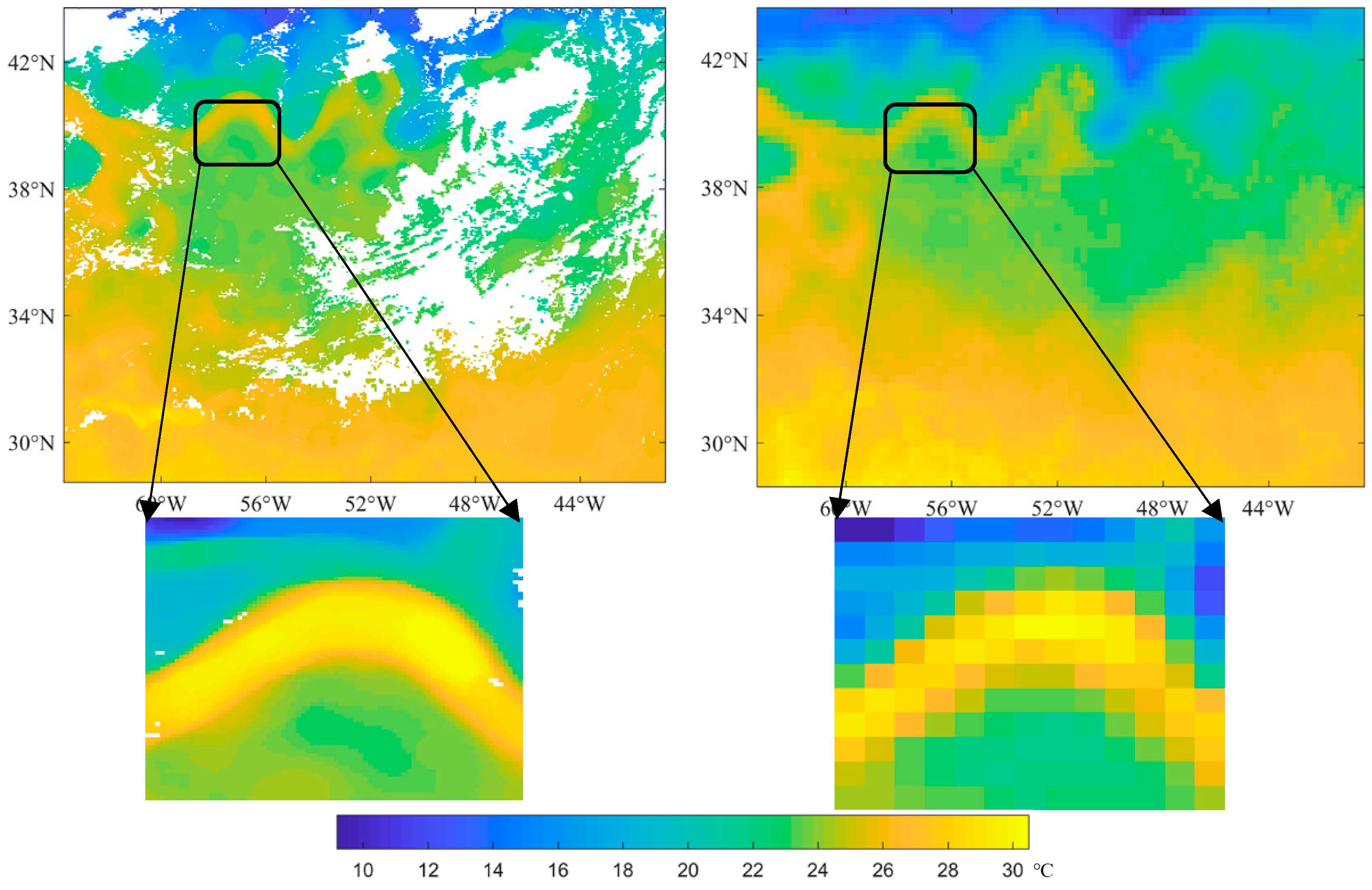
Meso- and fine-scale sea surface temperature (SST) is a key parameter for the research of the sub-mesoscale oceanic dynamic process, as well as the basic data for mesoscale oceanic front and eddy detection. The remote sensing technique is an efficient way to acquire global SST. Generally, there are two kinds of satellite-derived SST, including infrared-based SST, such as the moderate resolution imaging spectroradiometer (MODIS) data, and microwave-based SST, such as the advanced microwave scanning radiometer 2 (AMSR2) data. However, as shown in Figure 1, single infrared-based and microwave-based satellite-derived SST cannot obtain complete coverage and high-resolution SST simultaneously. Hence, complete and high-resolution SST reconstruction is an essential topic in oceanographical remote sensing. Multi-source SST fusion methods, such as the optimal interpolation method [1,2,3], and SST spatio-temporal reconstruction methods, such as the data interpolating empirical orthogonal functions (DINEOF) [4,5,6,7,8,9,10,11], are two main SST reconstruction methods. However, the optimal interpolation method may smooth small-scale features and the DINEOF method cannot reconstruct small-scale SST features contained in the nondominant EOF modes [12]. Therefore, meso- and small-scale SST features’ reconstruction becomes necessary.
With the arrival of the big data era, the deep learning super-resolution (SR) technique has exhibited its progressiveness in image resolution enhancement and has been widely used for natural pictures and remote sensing images to acquire clear and detailed maps [13,14,15,16,17,18,19,20,21,22,23,24,25,26,27,28]. The SR technique can enhance the resolution of low-resolution images and yet still preserve the meso- and small-scale details by multi-scale structure features’ learning. Due to the spatial similarity of infrared-based and microwave-based SST (Figure 1), it is possible to train an SR model based on these two satellite-derived SST data and then to enhance the resolution of low-resolution microwave-based SST using the trained model, thereby obtaining complete and high-resolution SST. According to the previous research [29], the SR technique can obtain better reconstruction accuracies than the bicubic interpolation method in four different oceanic regions.
Currently, the development of the SR technique is mainly focused on the structure improvement of the SR model, however, the training dataset could affect the SR performance. Commonly, the low-resolution images are first generated by downscaling the corresponding high-resolution images, and then the high- and simulated low-resolution images are used to train the SR models. In this study, the high- and low-resolution SST data are derived from two different sensors, so their structure similarities are lower than those of simulated images, which may affect the reconstruction accuracy. Hence, in this study, we discussed the influence of structure similarities of training patches on SST deep learning SR based on four classic SR models for four different oceanic regions.
In the remainder of the paper, the high- and low-resolution SST data and the SR models are introduced in Section 2; then, the experimental results are exhibited in Section 3, the performances of the training dataset selection strategy and different SR models on SST reconstruction are discussed in Section 4, and finally, a concise conclusion is provided in the last section.
2. Data and Methods
2.1. Experimental Data
The 3-day averaged AMSR2 SST data with spatial resolution of 0.25° from 2013 to 2019 were used as the low-resolution images in this study because of their relatively complete spatial coverage. They can be downloaded from Remote Sensing Systems (https://data.remss.com/amsr2/ocean/L3/, accessed on 7 September 2021). In addition, daily 4 km L3 mapped MODIS/Terra SST data covering the same period, downloaded from NASA Ocean Color Web (https://oceandata.sci.gsfc.nasa.gov/directaccess/MODIS-Terra/Mapped/Daily/4km/sst/, accessed on 7 September 2021), were selected as the high-resolution maps. To reduce the temporal difference, similar to the AMSR2 SST, the daily MODIS SST on the target date and two days before the target date were averaged to generate 3-day averaged MODIS SST. Then, the 3-day MODIS SST were filtered by a median filtering to eliminate the abnormal values. The SST data from 2013 to 2018 were used to train the SR models, and the SST data in 2019 were used as test data to assess the trained models. Since the AMSR2 data from 11 to 13 May 2013 and MODIS data from 19 to 24 February 2016 and 15 December 2016 are nonexistent, the total number of low- and high-resolution image pairs in the training and testing datasets is 2181 and 365, respectively.
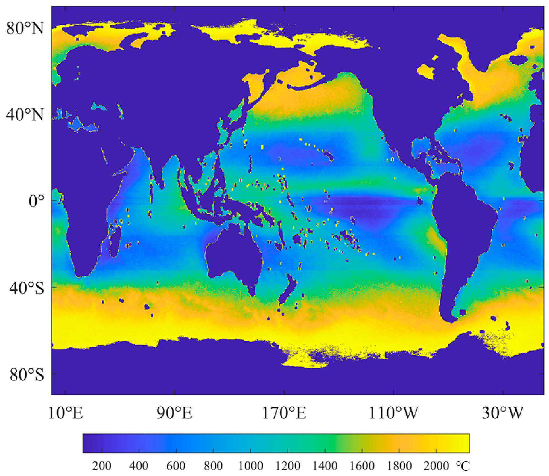
The AMSR2 data values less than 250 can be linearly transformed into actual SST with a slope of 0.15 and an intercept of −3, and values larger than 250 are deemed as missing or land pixels. In addition, the missing or land pixels in the MODIS data are already assigned to the NaN values. The number of missing pixels in either AMSR2 or MODIS SST for a given location in the training dataset was counted and the spatial distribution of missing data is shown in Figure 2. As shown in Figure 2, at the low latitudes, the influence of missing data is lower than that at the middle and high latitudes, which means the training patches are more likely derived from these regions.
There are two preprocesses before generating the training dataset, including: (1) the bicubic interpolation method, which was used to upscale the AMSR2 SST to the same size as MODIS SST, and (2) the MODIS data were shifted 180 degrees in longitude because of the spatial offset of 180 degrees in longitude between two experimental datasets. The size of training patches was set to 40 in this study and there is no spatial overlap among different patches. The total number of trainable pairs without missing data in the training dataset is 408,536. Due to the requirements of the Caffe package [30], all the training data were normalized into [0,1]. The structure similarity index (SSIM) was used to evaluate the structure similarities of training pairs. The SSIM can be calculated as follows:
where and are the mean values of the AMSR2 and MODIS training patches, denotes the covariance of the corresponding training patches, and are the standard deviations of the AMSR2 and MODIS patches, and C1, C2 are two small constants to avoid outliers.
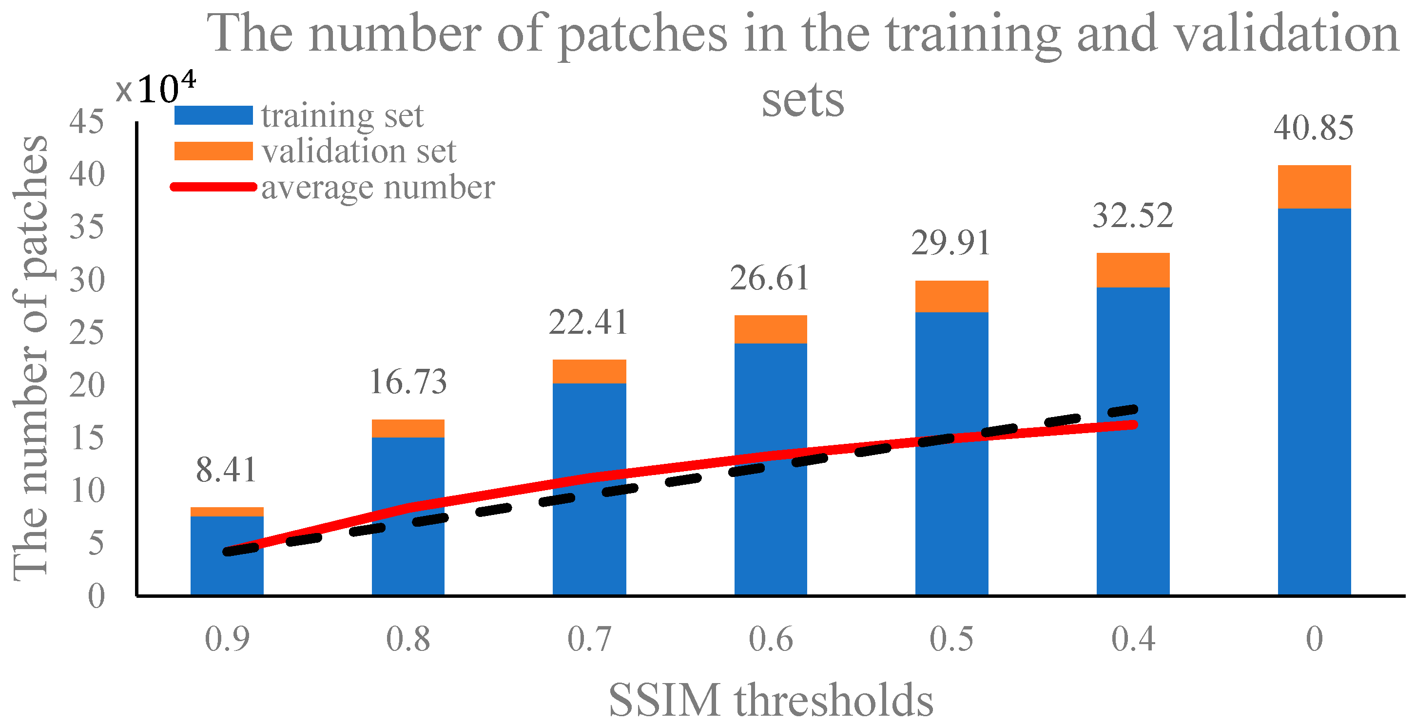
The AMSR2 and MODIS SST pairs in the training dataset have different SSIM values, so we used various SSIM thresholds to determine the corresponding training datasets for SR models’ training, which means the samples with SSIM values lower than the corresponding thresholds were discarded from the training set. The SSIM thresholds in this study were set to 0, and from 0.4 to 0.9 with an interval 0.1. In addition, 90% of the corresponding training pairs were randomly selected to form the training set and the rest were distributed into the validation set. The distribution of the number of training pairs in the training and validation sets with different SSIM thresholds is shown in Figure 3. As shown in Figure 3, with the decrease of the SSIM thresholds, the number of training pairs increases from 8.41 × 10⁴ to 40.85 × 10⁴. The red line in Figure 3 represents the trend of the average number of training pairs with different SSIM thresholds and the black dotted line is the 1:1 line. We can see that when the SSIM thresholds vary from 0.9 to 0.5, the enhancement of the number of training pairs surpasses the 1:1 line, however, when the SSIM thresholds are less than 0.5, the enhancement is below the 1:1 line. In addition, more than 73% of training pairs have SSIM values greater than 0.5. Hence, we can deduce that most training pairs have relatively large SSIM values.
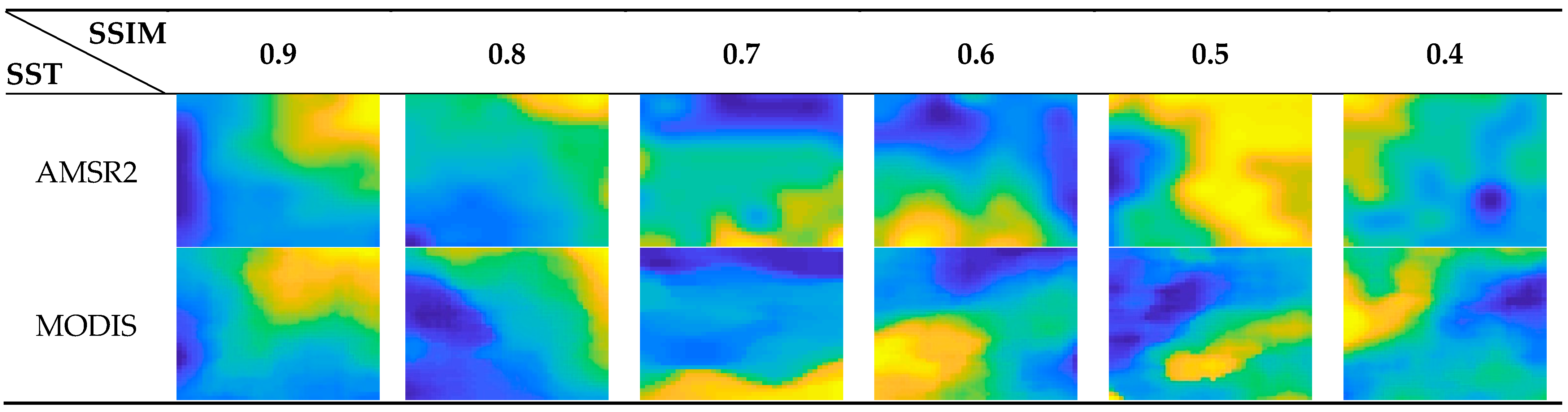
The examples of the AMSR2 and MODIS SST patches with different SSIM values in the training set are shown in Figure 4. As shown in Figure 4, the SSIM value can effectively mirror the structure features of training patches. Since the deep learning SR technique enhances the resolution of low-resolution images by multi-scale structure features’ learning, a suitable training set determined by the SSIM value is necessary for SST SR reconstruction.
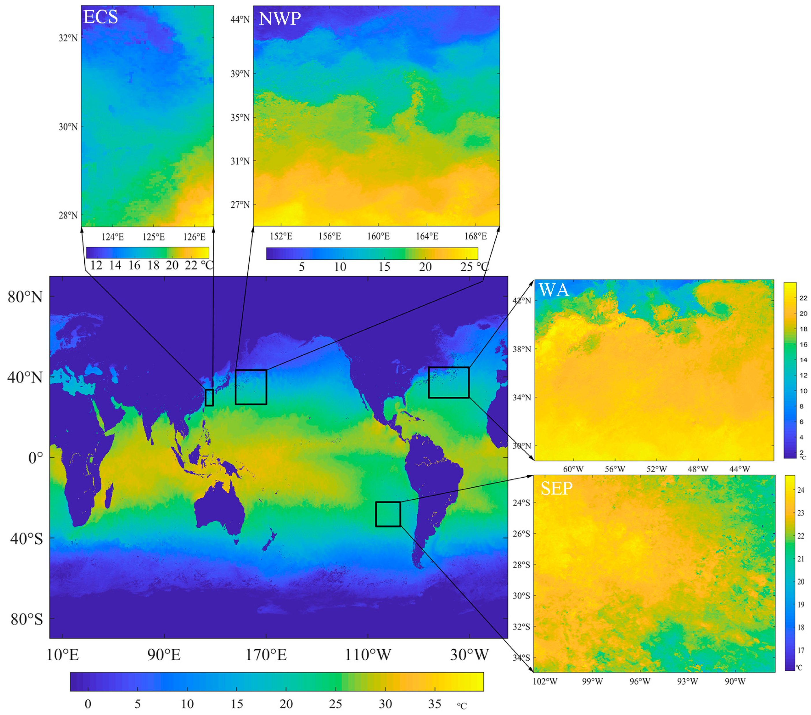
At the test stage, in this study, four representative areas (Figure 5) were chosen to evaluate the performances of the selected SR models. The East China Sea (ECS), a marginal sea east of China, was selected as the first experimental area, covering from 123.27°–126.48°E to 27.77°–32.73°N. The second and the third areas are in the northwest Pacific (NWP), ranging from 149.77°–169.98°E to 25.02°–45.23°N, and in the west Atlantic (WA), ranging from 40.77°–63.73°W to 28.77°–43.73°N, respectively. The variations of SST in these two regions are noticeable. The last one is in the southeast Pacific (SEP) covered by less varied SST, ranging from 87.52°–102.73°W to 22.27°–34.98°S.
Overall, the average percentages of missing data in the testing dataset for AMSR2 and MODIS SST are 1.18% and 47.40%, respectively. As shown in Table 1, due to the influence of microwave radiation from the land, the percentage of missing data for AMSR2 SST in ECS is greater than 2%, and yet for the rest of the experimental regions, the percentages of missing data are all less than 1%. In addition, the percentages of missing data for MODIS SST in the four experimental areas are all greater than 40%, ranging from 41.77% in SEP to 54.19% in NWP. Since complete SST input is necessary for SST SR, the linear interpolation method was employed to complete the input for AMSR2 SST.
2.2. SR Models
In this study, we selected four classical deep learning SR models, including the super-resolution convolutional neural network (SRCNN), the deep recursive residual network (DRRN), the symmetrical dilated residual convolution networks (FDSR), and the oceanic data reconstruction network (ODRE), for SST reconstruction. The codes of SRCNN and DRRN models were downloaded directly from GitHub (https://github.com/SolessChong/srcnn-caffe; https://github.com/tyshiwo/DRRN_CVPR17, accessed on 7 September 2021) and the codes of FDSR and ODRE models were accomplished based on the published manuscripts of [29,31]. All these models can be considered as early up-sampling methods, which means the bicubic interpolation is used first to upscale the low-resolution input to the same size as the high-resolution output. Though the late up-sampling methods, in which the nonlinear convolutions are operated directly in low-resolution space, can be more efficient, they are probably not suitable for SST reconstruction. In the late up-sampling methods, the low-resolution input, i.e., AMSR2 SST, should be large enough to extract features, however, due to the large scaling factor (about ×6) and the missing data in the high-resolution output, i.e., MODIS SST, the number of trainable patches will be reduced. For example, if the size of AMSR2 SST patches is 40 × 40, the size of the corresponding MODIS SST patches will be approximately 240 × 240. The number of MODIS SST patches with size of 240 × 240 and without missing data is relatively small, so the number of trainable pairs may be insufficient for model training. Hence, only early up-sampling methods were used in this study. Next, we briefly introduce these four SR models.
2.2.1. Super-Resolution Convolutional Neural Network (SRCNN) Model
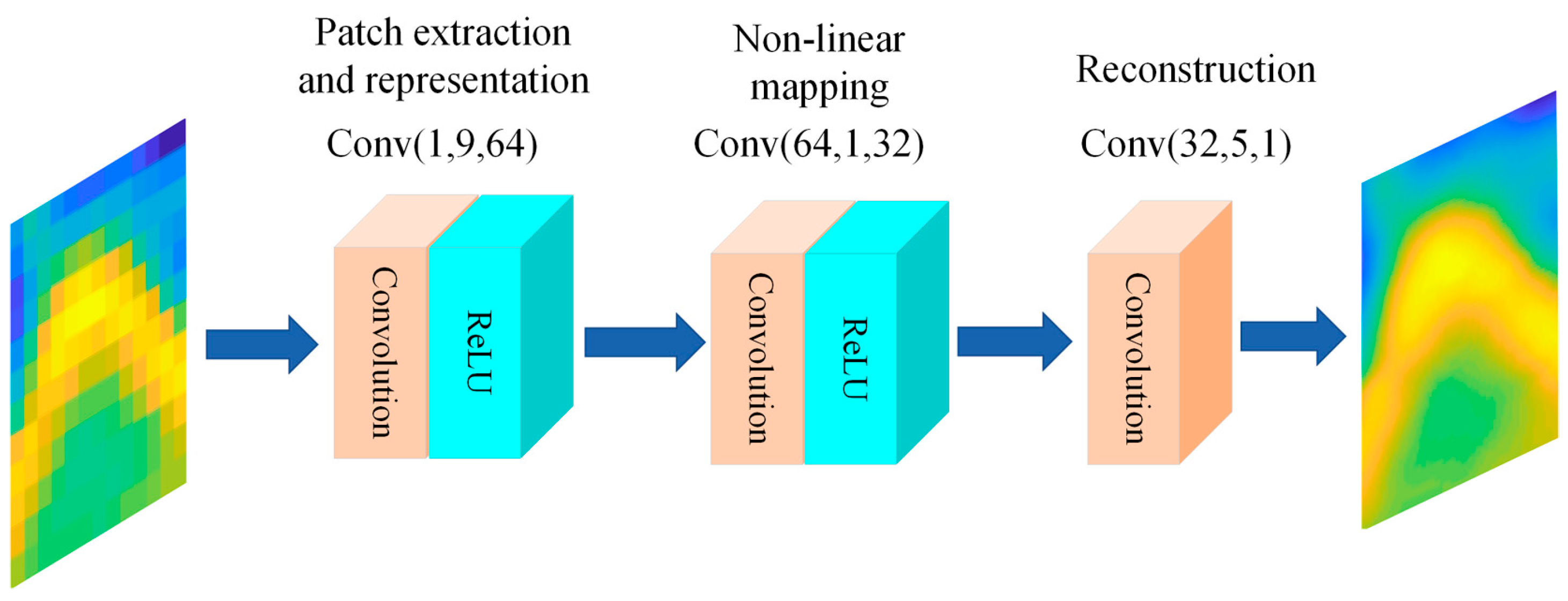
Dong et al. [32] proposed the SRCNN model, which can be deemed as the first SR model based on deep learning. As shown in Figure 6, it has three convolution layers for patches’ extraction and representation, non-linear mapping, and reconstruction. The outputs of the first two convolution layers are nonlinear transformed by using the rectified linear unit (ReLU) layer. Similar to the previous study [32], in this study, the kernel sizes in these three convolution layers are 9, 1, and 5, and the number of the output channels in each convolution layer is 64, 32, and 1. The numbers in the brackets in Figure 5 denote the number of the input channel, the kernel size, and the number of the output channel in sequence.
2.2.2. Deep Recursive Residual Network (DRRN) Model
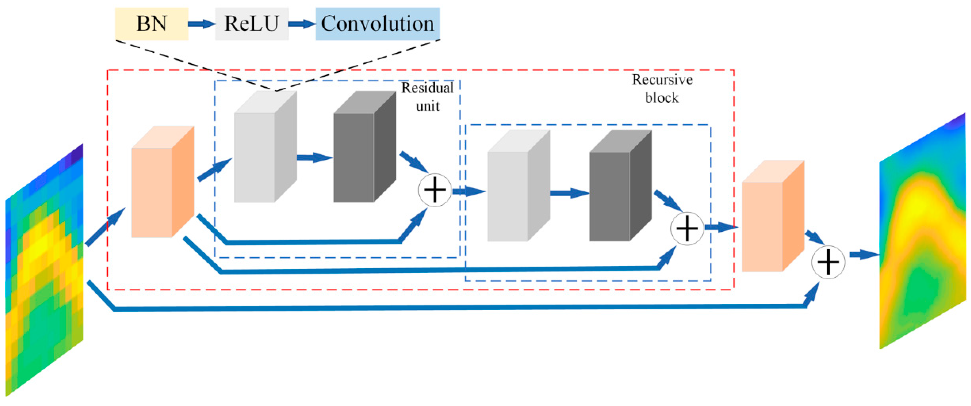
Tai et al. [33] proposed the DRRN model for single-image SR. As shown in Figure 7, the basic structure of DRRN is a recursive block containing several residual units. Three stacked layers, including a batch normalization (BN) layer, a ReLU activation layer, and a convolution layer, in sequence, form a group. The input of the recursive block is first processed through a group and the result, H, is used as the input of each residual unit based on multi-path mode. There are two groups in each residual unit, and the weight sharing strategy is used for each residual unit within a recursive block. The output of the second group in a residual unit is added to the result, H, as the input for the next residual unit. There is a group at the end of DRRN to reconstruct the residual between the low- and high-resolution images, and then the residual image is added to the original input to acquire the final high-resolution map. The number of recursive blocks, Nb, and the number of residual units, Nu, in each recursive block are two key parameters of DRRN, and the depth, d, of the network is determined by these two parameters, as follows:
In this study, we used the same parameters as the original manuscript, i.e., Nu is 9 and Nb is 1. The kernel size in all convolution layers is 3, and except for the first and the last convolution layers of DRRN, the input and output channels in all convolution layers are set to 64.
2.2.3. Symmetrical Dilated Residual Convolution Networks (FDSR) Model
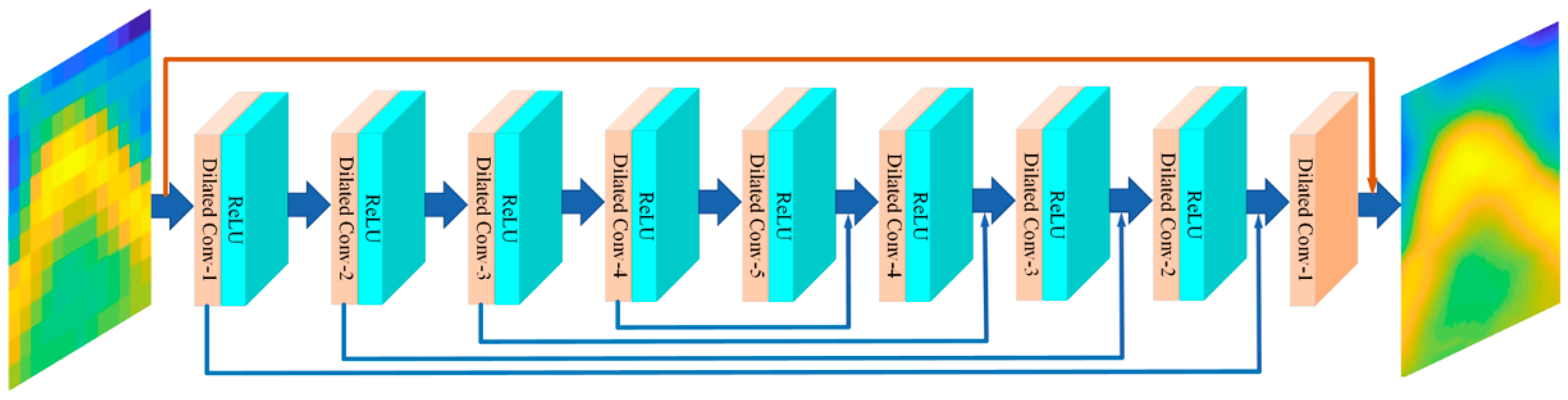
The FDSR model was proposed by Zhang et al. [31] for single-image SR. As shown in Figure 8, the main structure of FDSR contains cascade dilated convolution layers followed by the ReLU layers, and skip connections (blue line) are used to link the symmetrical dilated convolution layers. Global residual learning (red line) is also used in FDSR. The kernel size of all convolution layers is set to 3, and to maintain the output image size, the dilation factor and the zero-padding in each layer are both set to 1, 2, 3, 4, 5, 4, 3, 2, 1. Hence, the receptive field of each layer is 3, 7, 13, 21, 31, 39, 45, 51, 55. Except for the first and the last convolution layers, the input and output channels in all convolution layers are set to 64.
2.2.4. Oceanic Data Reconstruction Network (ODRE) Model
The ODRE model proposed by Ping et al. [29] aims to reconstruct low-resolution SST images using the deep learning SR technique. As shown in Figure 9, there are two parts in ODRE, including multi-scale features’ extraction and multi-receptive field mapping. In the multi-scale features’ extraction, three convolution layers with kernel size 3, 5, and 7 are used to extract oceanic features. The ReLU layer is then employed for non-linear transformation. The outputs of multi-scale features’ extraction are concatenated, and a bottleneck layer with 1 × 1 convolution is used to shrink the channels down to 64. The multi-receptive field mapping part is similar to the FDSR model except the largest dilation factor is set to 4. Except for the first and the last convolution layers and the bottleneck layer, the input and output channels in all convolution layers are set to 64.
2.3. Network Training
In this study, the average squared error was utilized as the loss function for all selected models, and the loss function was optimized by using the mini-batch gradient descent algorithm with back-propagation. Due to the lack of global residual learning, Equation (3) is the loss function of the SRCNN model and Equation (4) is the loss function of the other three models:
where p and q indicate the upscaled AMSR2 and actual MODIS SST respectively, f is the selected SR models, and N represents the number of training pairs in a mini-batch, and it was set to 64 in this study. All SR models were trained using the corresponding training datasets for up to 100 epochs. In addition, the convolutional filters in the DRRN, FDSR, and ODRE models were initialized by using “MSRA” [26] and in the SRCNN model were initialized by using “gaussian”. The initial learning rates of the SRCNN model and the other three models are 1 × 10⁻⁵ and 1 × 10⁻⁶ respectively, and they are all halved after 50 epochs.
2.4. Quantitative Evaluation
Three indices, including the root mean squared error (RMSE), the mean absolute error (MAE), and the peak signal-to-noise ratio (PSNR), were used to analyze the performances of the trained SR models based on the actual MODIS SST in the testing dataset and the corresponding reconstructed SST. For clarification, the smaller MAE and RMSE values and the higher PSNR value signify better-reconstructed performance. The RMSE, MAE, and PSNR can be calculated as follows:
where r and a represent the reconstructed SST and the actual MODIS SST, s indicates the existing pixels in SST images, m indicates the maximum value, and {} is the number of elements in a set.
3. Results
3.1. Statistical Results
In this section, we calculated the RMSEs, MAEs, and PSNRs for the four experimental regions using the selected SR models trained based on different training datasets determined by various SSIM thresholds.
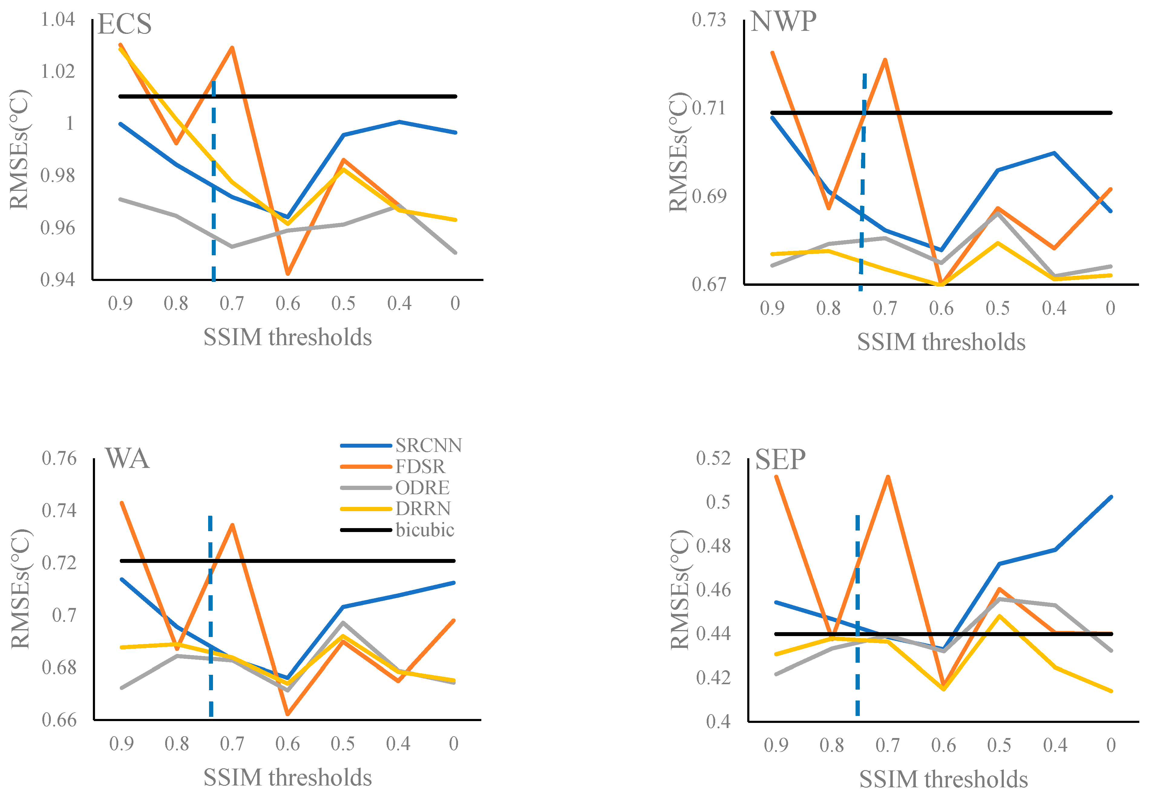
3.1.1. RMSEs in Four Regions
The RMSEs for the four experimental regions obtained from the selected SR models trained based on different training datasets determined by various SSIM thresholds are shown in Figure 10. Generally, the SR models trained using the training dataset determined by the SSIM value of 0.6 can acquire relatively lower RMSEs (blue dotted line) for the four experimental regions. The amplitudes of variations of RMSEs from the FDSR model (orange line) are the largest with different training datasets, ranging from 0.94 to 1.03 in ECS, from 0.67 to 0.72 in NWP, from 0.66 to 0.74 in WA, and from 0.42 to 0.51 in SEP. In addition, the ODRE (green line) and DRRN (yellow line) models seem to be less affected by the training dataset. For the ODRE model, the RMSEs range from 0.95 to 0.97 in ECS, from 0.67 to 0.69 in NWP, from 0.67 to 0.70 in WA, and from 0.42 to 0.46 in SEP. For the DRRN model, the RMSEs range from 0.96 to 1.03 in ECS, from 0.67 to 0.68 in NWP, from 0.67 to 0.69 in WA, and from 0.41 to 0.45 in SEP. In most cases, compared with the bicubic interpolation method (black line), the SR models can obtain lower RMSEs in ECS, NWP, and WA, where the SST variations are relatively large, and yet in SEP where SST is more stable, the superiority of SR models is not as obvious as that in the other three regions. The SR technique can enhance the spatial resolution of low-resolution images by multi-scale structure features’ learning, so the SR models may be more practical for the regions with large SST spatial variations because of the apparent SST structures.
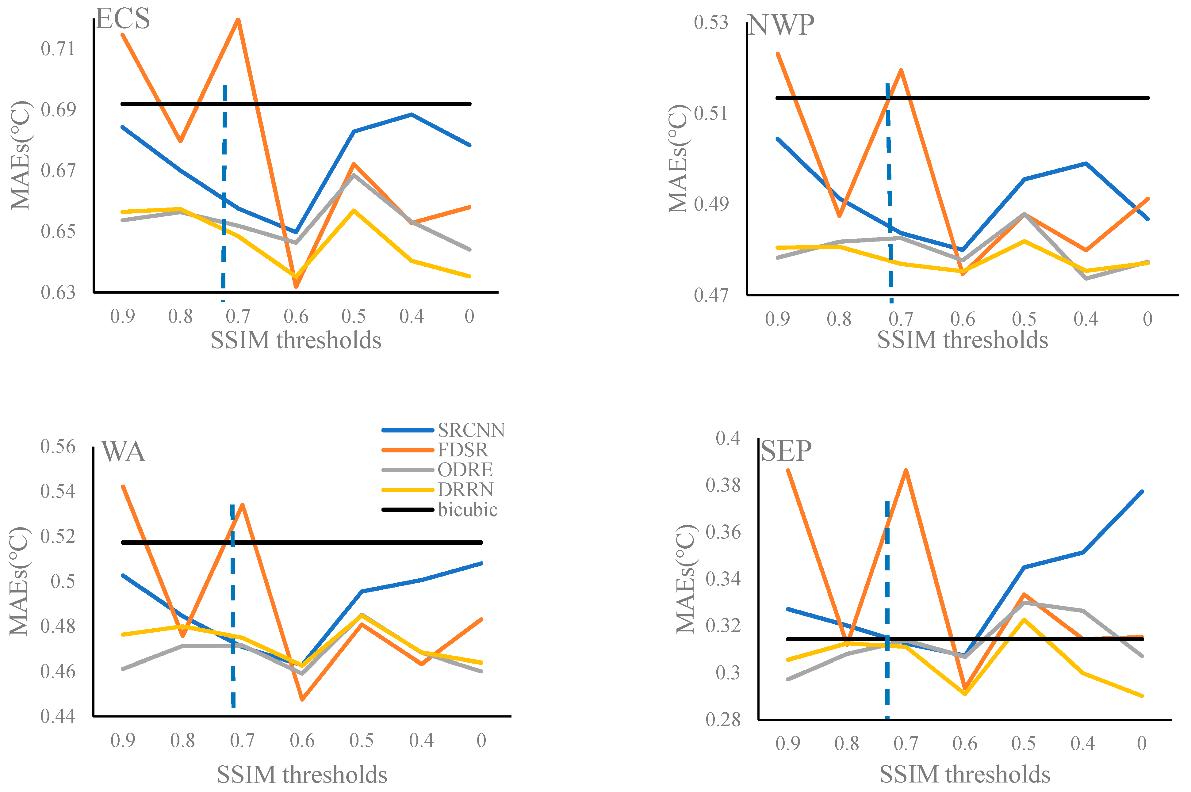
3.1.2. MAEs in Four Regions
As shown in Figure 11, similar to the RMSEs, the training dataset determined by the SSIM value of 0.6 is the most suitable for SR training due to the lowest MAE values for the four experimental regions. In addition, the FDSR model is the most sensitive to the training dataset with MAEs ranging from 0.63 to 0.72 in ECS, from 0.47 to 0.52 in NWP, from 0.45 to 0.54 in WA, and from 0.29 to 0.39 in SEP. The MAEs obtained from the ODRE and DRRN models are more stable. For the ODRE model, the MAEs range from 0.64 to 0.67 in ECS, from 0.47 to 0.49 in NWP, from 0.46 to 0.49 in WA, and from 0.30 to 0.33 in SEP, and for the DRRN model, the MAEs range from 0.64 to 0.66 in ECS, from 0.47 to 0.48 in NWP, from 0.46 to 0.48 in WA, and from 0.29 to 0.32 in SEP. In ECS, NWP, and WA, except for the FDSR model, the SR models have better performances than the bicubic interpolation method for all training datasets. In SEP, all SR models trained using the training dataset determined by the SSIM value of 0.6 can obtain lower MAE values than the bicubic interpolation method.
In conclusion, the training datasets determined by different SSIM thresholds can affect SR model training, and consequentially, affect the SST reconstruction. From the point of reconstruction accuracy, an SSIM value of 0.6 is a good choice for the SST training dataset determination, which can ensure that high- and low-resolution SST training pairs in the training dataset are structurally similar, and still provide sufficient data for SR model training.
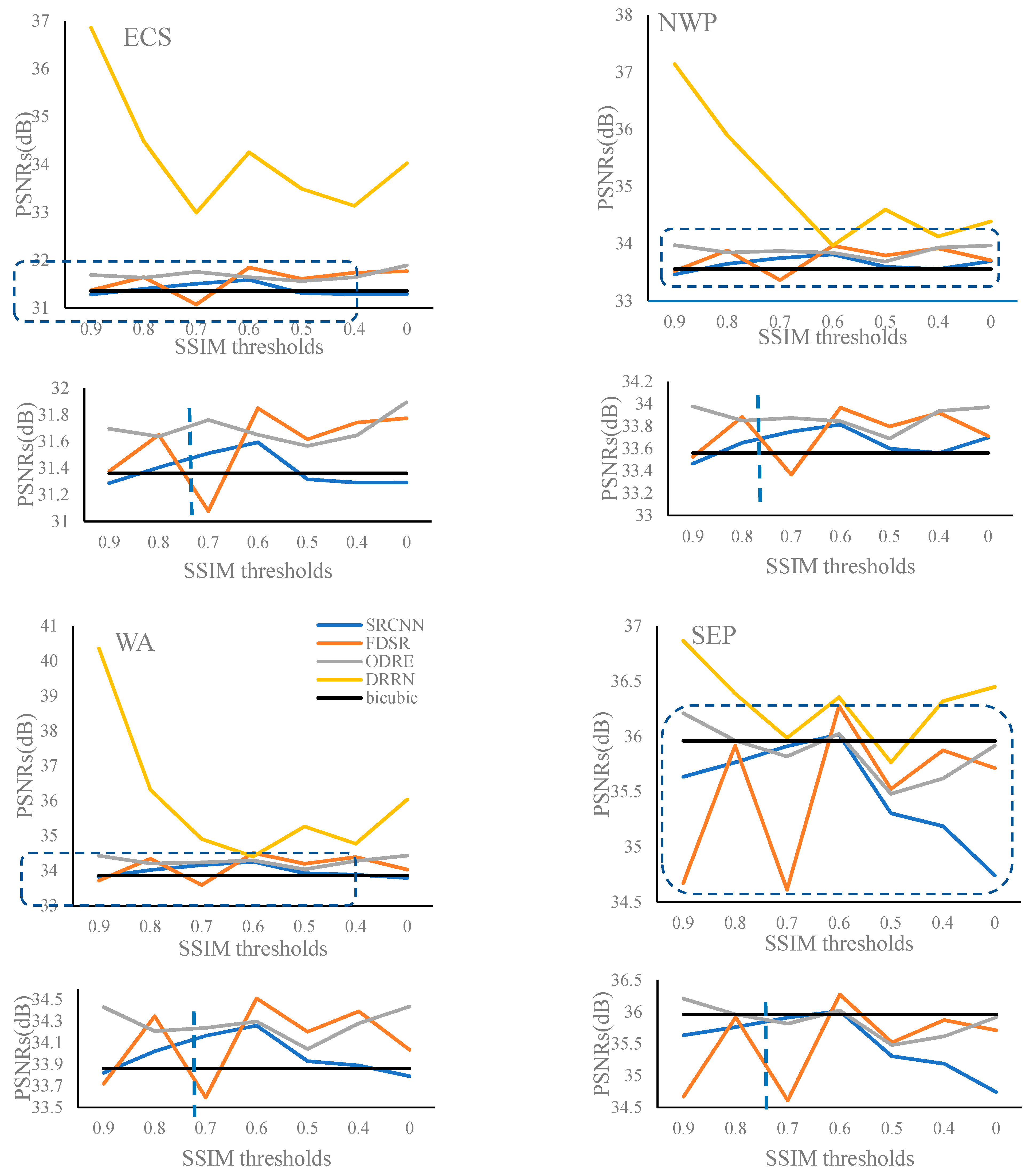
3.1.3. PSNRs in Four Regions
As shown in Figure 12, compared with the other three models, the DRRN model has the highest PSNRs for the four experimental regions, which complies with the “the deeper, the better” conception proposed by Kim et al. [14]. For better comparison, the distributions of PSNRs from the other three models (black dotted square) are enlarged below the corresponding images. Generally, the DRRN model trained using the training dataset determined by relatively large SSIM thresholds can acquire high PSNRs, however, when the SSIM threshold decreases to 0.7, the PSNRs from the DRRN model are stable for the four experimental regions, and meanwhile, the differences of PSNRs obtained from these four SR models are reduced in NWP, WA, and SEP. Except for the DRRN model, the amplitudes of variations of PSNRs from the FDSR model are relatively larger than those from the SRCNN and ODRE models. For the FDSR model, the PSNRs range from 31.08 to 31.85 in ECS, from 33.37 to 33.97 in NWP, from 33.59 to 34.51 in WA, and from 34.61 to 36.28 in SEP.
In addition, except for the DRRN and ODRE models, the other two SR models trained using the training dataset determined by the SSIM value of 0.6 can acquire higher PSNR values. Actually, the ODRE model with the SSIM value of 0.6 can still obtain a comparable PSNR value. Compared with the bicubic interpolation method (black line), in most cases, the SR models can obtain higher PSNRs in ECS, NWP, and WA, where SST is less uniform. However, in SEP, where the variation of SST is not obvious, training dataset selection is necessary and the SSIM value of 0.6 is a reasonable option.
In summary, to balance the reconstruction errors (RMSE and MAE) and image quality (PSNR), the training dataset determined by the SSIM value of 0.6 was recommended and selected in this study.
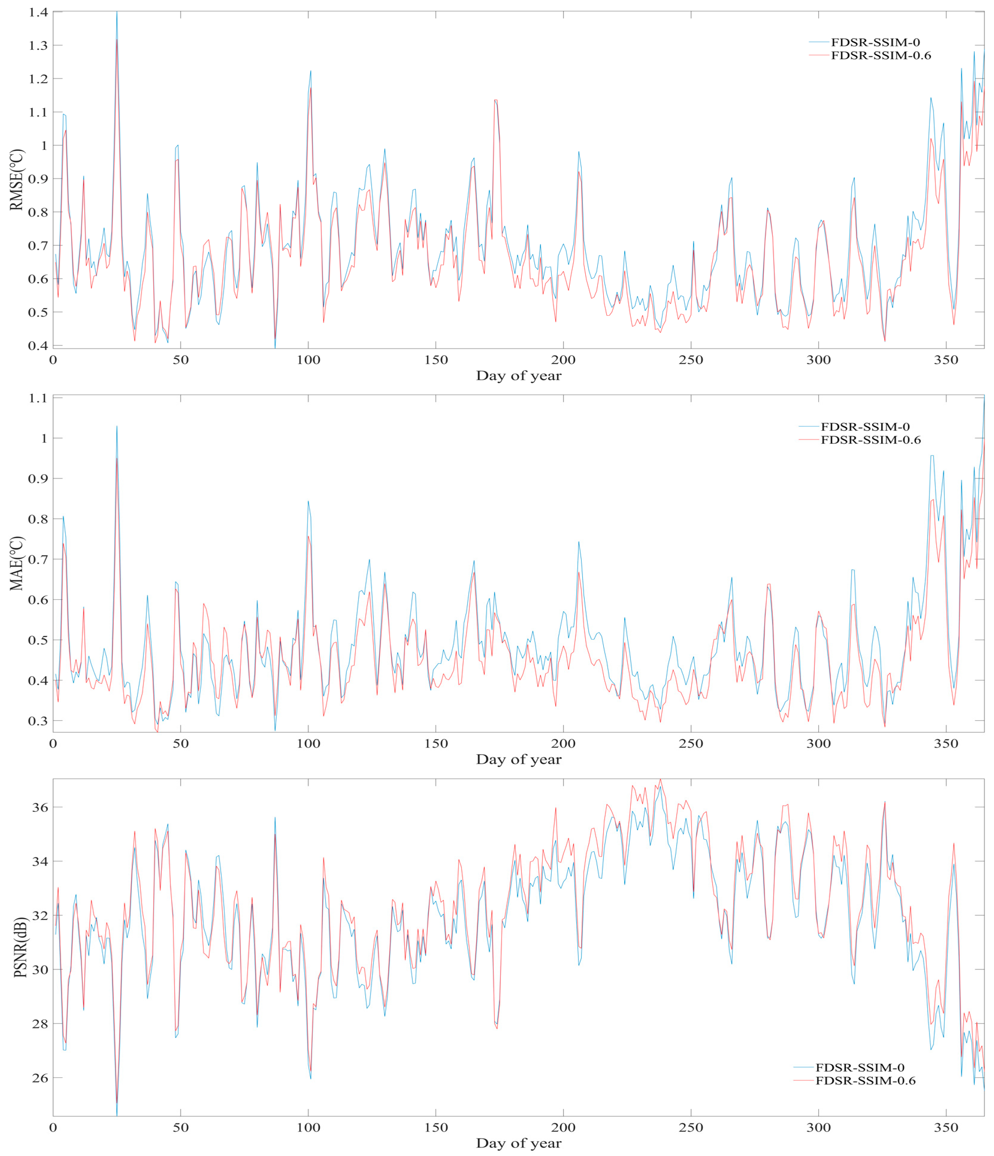
3.2. Daily Differences Based on Different Training Datasets
To better exhibit the necessity of training dataset selection, in this section, we selected the WA region as an example to show the daily differences obtained from the FDSR model trained using the 0 and 0.6 SSIM datasets. As shown in Figure 13, we can see that the trends of RMSEs, MAEs, and PSNRs based on these two training datasets are in general quite similar. In most cases, the FDSR model trained using the 0.6 SSIM dataset results in lower RMSEs as well as MAEs and higher PSNRs, which indicates that compared with the training based on the 0 SSIM dataset (without SSIM determination), the training dataset selection can improve the reconstruction accuracy.
3.3. A Case Study
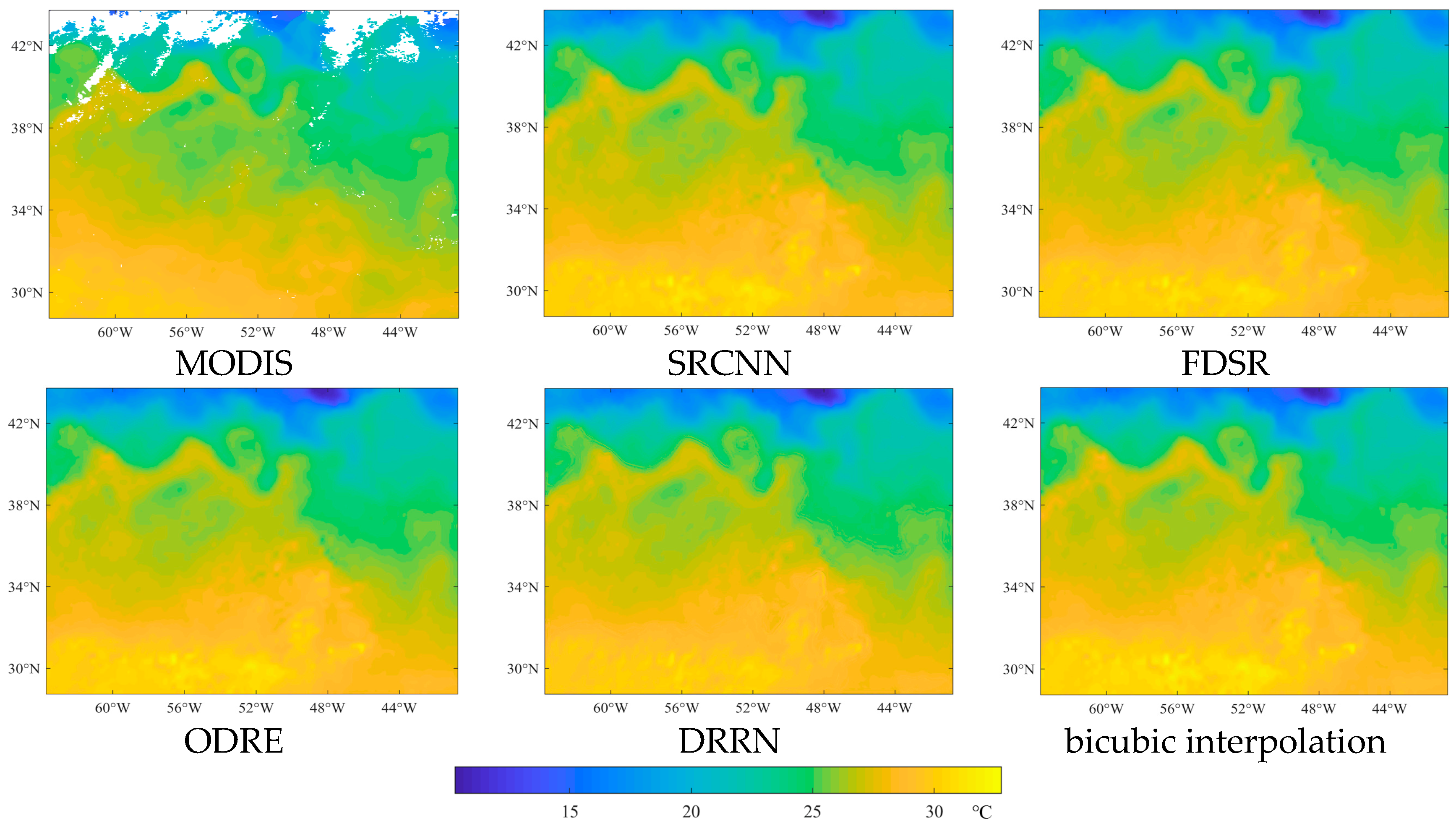
As shown in Figure 14, the original MODIS SST with missing pixels in WA on 25 July 2019, and its reconstructed SST obtained from the SR models and the bicubic interpolation method, were used as an example to make a visual comparison. The SR models were trained using the dataset determined by the SSIM value of 0.6. Generally, the reconstructed SST images obtained from different SR models and the bicubic interpolation method are visually similar, and the main spatial structure of SST is suitably reconstructed. The main reason is that the details of SST are not so abundant as those in the natural images, so the SST reconstructions with different SR models are visually similar. However, it is noteworthy that similar spatial structure does not mean similar reconstruction accuracy.
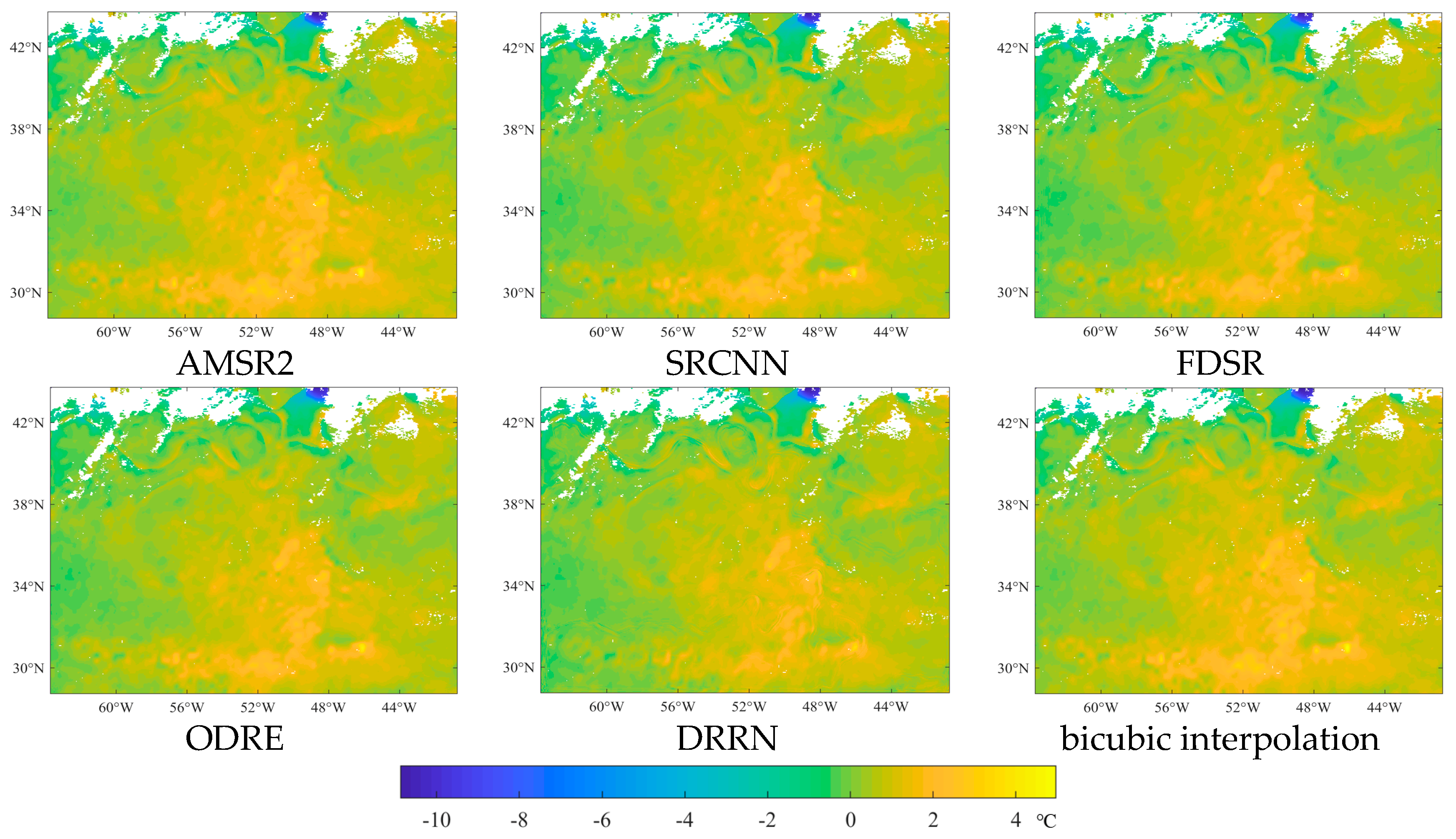
The differences between the up-sampled AMSR2 SST image as well as the reconstructed SST images and the original MODIS SST image are shown in Figure 15. We can see that the reconstructed SST in the middle of the image is higher than the original SST, and the largest negative difference can be found around clouds. In addition, the difference between the up-sampled AMSR2 SST and the original MODIS SST has a significant impact on the difference between the reconstructed SST and the original MODIS SST, which means at the practical stage, the spatial similarity between the low-resolution input and the objective high-resolution output is a key factor influencing the SR reconstruction.
4. Discussion
4.1. Training Dataset Obtained from Single MODIS SST
In this section, we discuss another SR training strategy, i.e., instead of generating the training dataset based on the AMSR2 and MODIS SST fields (referred to as the original strategy), the training dataset was generated only based on the MODIS SST field (referred to as the simulation strategy). First, the MODIS SST were downscaled by using the local mean method and a scaling factor of 6, and then the downscaled SST were up-sampled to the original size by bicubic interpolation. The original MODIS SST and the simulated SST were used as high- and low-resolution SST to train the SR models. The size of the training patches was set to 40 with no spatial overlap among different patches. Training patches with missing data were excluded and the remaining training pairs were divided by 9:1 to form the training and validation sets. The number of training pairs in the training and validation sets is 444,792 and 49,980, respectively. Since the low-resolution SST images are generated based on the corresponding high-resolution MODIS SST, it is not necessary to select a training dataset based on structure similarity.
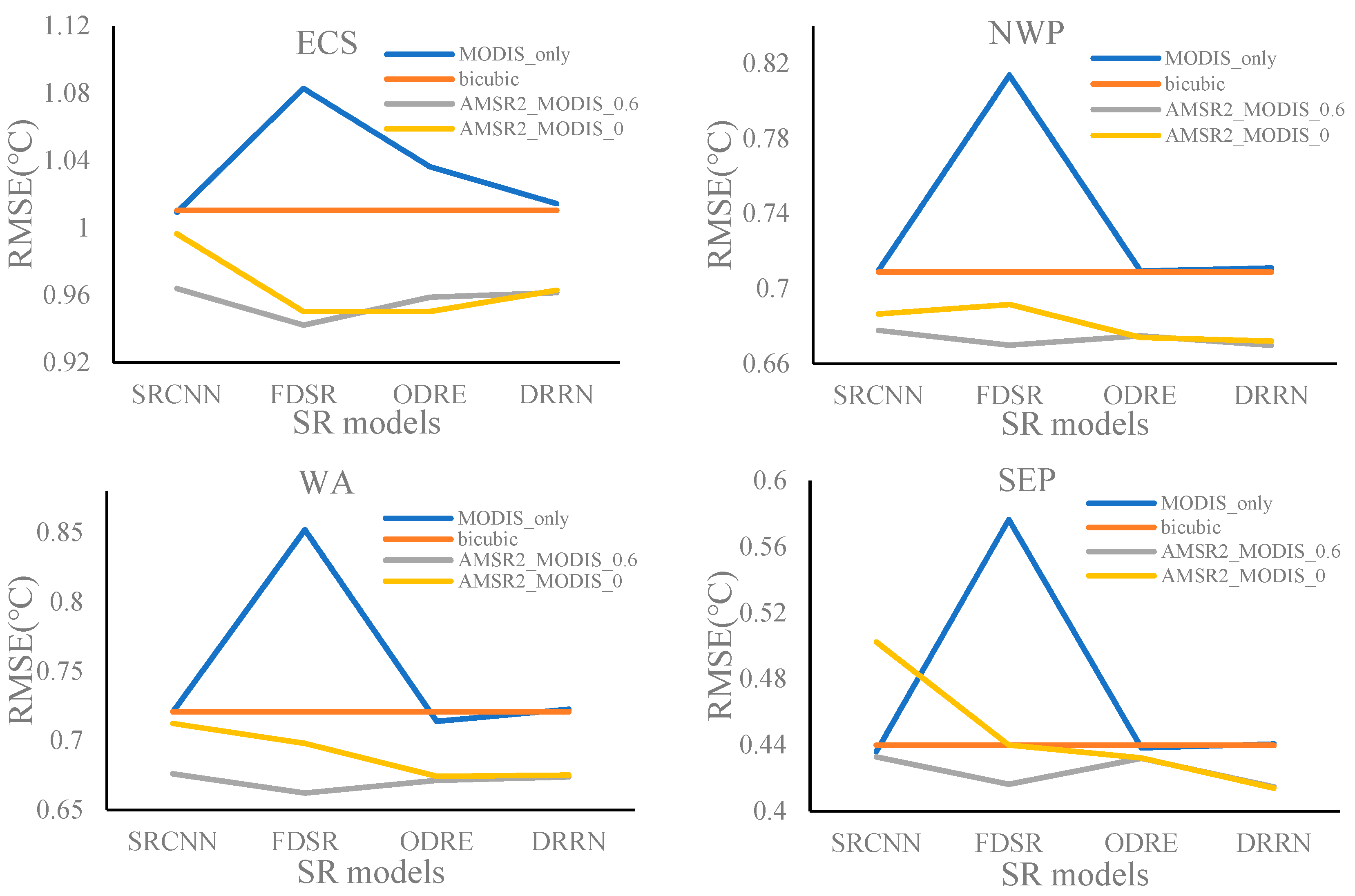
As shown in Figure 16, the RMSEs obtained from the simulation strategy (blue line) are all larger than those obtained from the original strategy in ECS, NWP, and WA, even than the 0 SSIM training set (yellow line) in the original strategy. In SEP, the original strategy based on the 0.6 SSIM training set results in lower RMSEs for all SR models, and except for the SRCNN model, the original strategy based on the 0 SSIM training set also results in better reconstruction accuracy. In addition, in most cases, the RMSEs obtained from the simulation strategy are higher than the bicubic interpolation method, especially for the FDSR model.
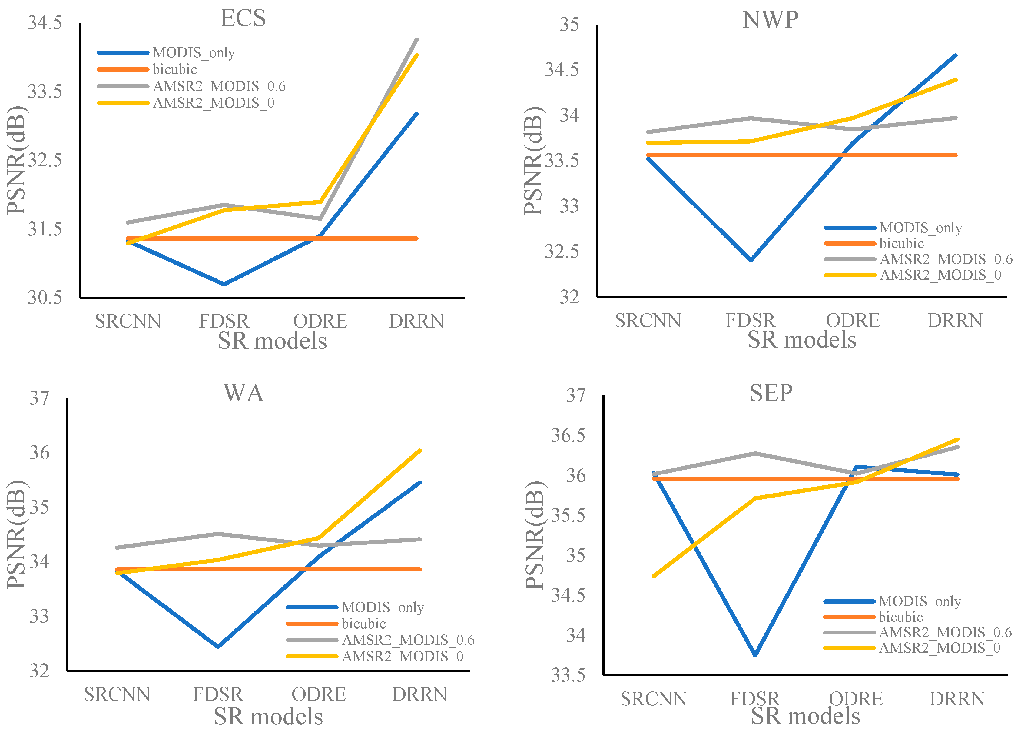
As shown in Figure 17, compared with the simulation strategy, except for the DRRN model, the original strategy with SSIM values of 0 and 0.6 results in higher PSNRs in NWP and WA. In ECS, the original strategy with SSIM values of 0 and 0.6 both acquire higher PSNRs than the simulation strategy for all the SR models. In SEP, the FDSR and DRRN models result in higher PSNRs. In addition, for the simulation strategy, the PSNRs from the FDSR model are lower than the bicubic interpolation method, and the DRRN model results in relatively higher PSNRs than the bicubic interpolation method. The differences between the other two models and the bicubic interpolation method are not obvious for the four experimental regions.
Hence, we can conclude that the training dataset obtained from the actual low- and high-resolution SST images is more suitable for SST SR. Actually, there is a temperature difference between the skin SST measured by the infrared radiometer and the sub-skin SST measured by the microwave radiometer. This difference can be reduced through the multi-source SST learning process, however, when the low-resolution SST images are simulated based on the high-resolution SST, the temperature difference cannot be effectively learned and reduced. In addition, the footprint of simulated low-resolution SST derived from the MODIS product is different from that of real AMSR2 SST, which may have an adverse influence on SST reconstruction. The AMSR2-MODIS datasets will take the footprint problem into account.
4.2. The Comparisons between Different SR Models
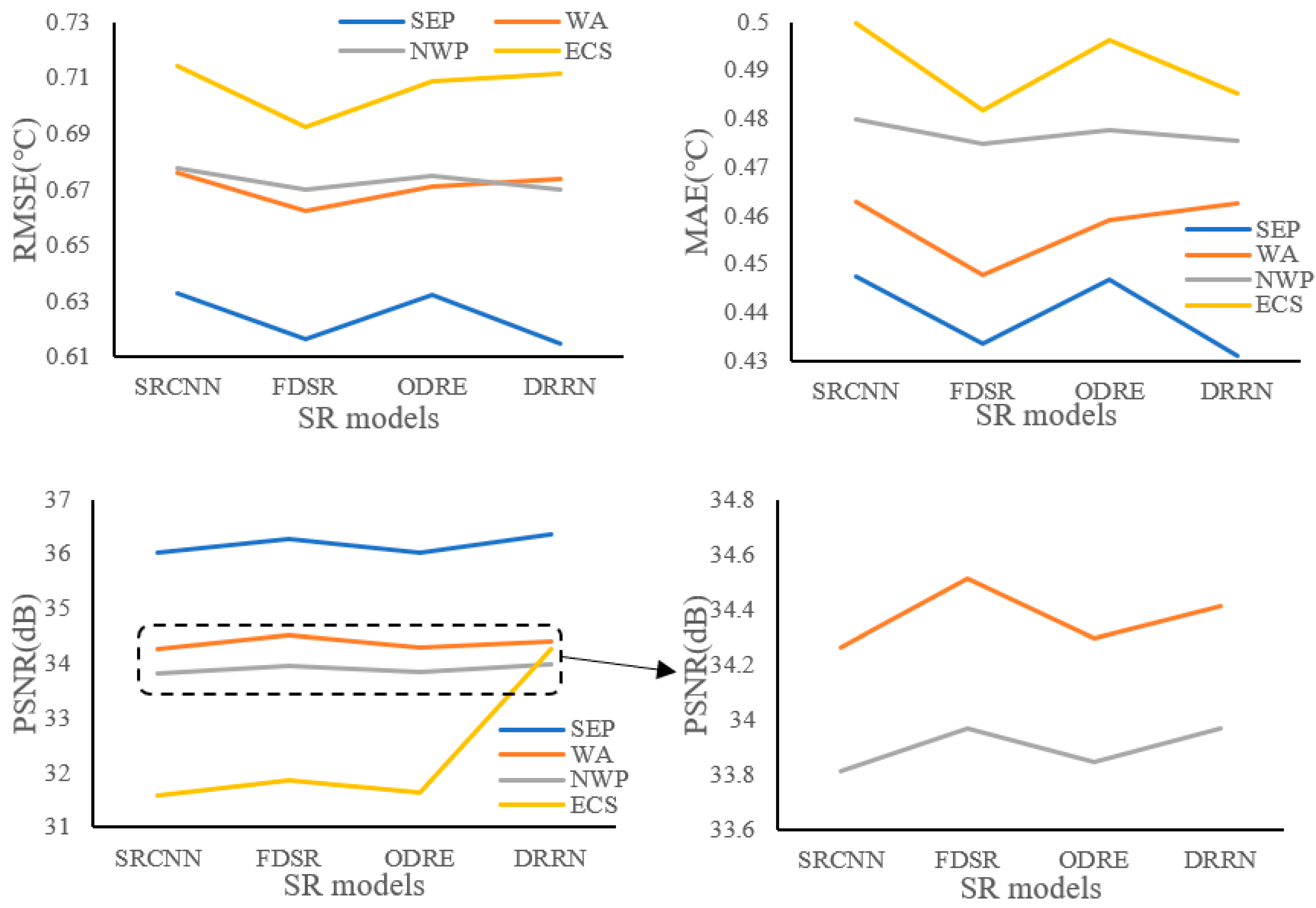
We used the 0.6 SSIM training set to train the four SR models, and then the statistical indices were employed to make comparisons between these SR models. To facilitate the comparison, 0.2 °C was added to the original RMSEs for SEP and 0.25 °C was subtracted from the original RMSEs for ECS. Similarly, 0.14 (0.15) °C was added to (subtracted from) the original MAEs for SEP and ECS, respectively. The statistical indices with these offsets are shown in Figure 18. As is evident in the figure for NWP and SEP, the FDSR and DRRN models resulted in relatively lower RMSE values, and in ECS and WA, the FDSR model resulted in the lowest RMSE values. Similarly, the FDSR and DRRN models obtained lower MAEs in ECS, NWP, and SEP, and the FDSR model obtained the lowest MAE in WA.
The PSNRs obtained in WA and NWP (black dotted square in Figure 18) are enlarged and shown next to the original image. Generally, except for the ECS (yellow line), the distributions of PSNRs obtained from the other three regions are similar, i.e., the FDSR and DRRN models resulted in relatively higher PSNR values. In ECS, the distributions of PSNRs obtained from the SRCNN, FDSR, and ODRE models are similar to those in the other three regions, however the DRRN model resulted in a higher PSNR value in ECS, which means that the DRRN model may be more suitable for marginal seas.
In addition, the largest differences of RMSEs and MAEs between these four SR models were 2.18 × 10⁻² °C and 1.79 × 10⁻² °C in ECS, 0.8 × 10⁻² °C and 0.53 × 10⁻² °C in NWP, 1.39 × 10⁻² °C and 1.52 × 10⁻² °C in WA, and 1.81 × 10⁻² °C and 1.63 × 10⁻² °C in SEP. Additionally, the largest difference of PSNRs was 2.66 in ECS, 0.16 in NWP, 0.25 in WA, and 0.34 in SEP. Hence, we can see that the SST reconstruction accuracies (RMSE and MAE) obtained from different SR models for the four experimental regions were relatively consistent, yet the differences in image quality (PSNR) were rather significant.
5. Conclusions
Deep learning SR has been widely used for enhancing the resolution of natural images and remote sensing images. Currently, most studies focus on improving the structure of the SR model, yet training dataset selection is largely ignored. Commonly, the high-resolution images in the training dataset are first downscaled to simulate the corresponding low-resolution images, and then the low- and high-resolution images are used to train the SR models. However, for SST SR, the low- and high-resolution SST are derived from different sensors, so the influence of the structure similarities of training patches on SST SR performance should be analyzed. In this study, we first discussed the necessity of training dataset selection for SST SR. Then, through reconstructing AMSR2 SST in four different regions, a suitable SSIM threshold for the training dataset selection was determined. In addition, visual comparisons between the reconstructed SST and the original MODIS SST were analyzed. Furthermore, two training dataset generation strategies were compared. Finally, the SST SR performances among four selected SR models were discussed. In summary, the conclusions are summarized as follows:
- (1)
- The training dataset determined by a SSIM value of 0.6 generally resulted in the lowest RMSEs as well as MAEs, and the highest PSNRs for the four experimental areas.
- (2)
- SR reconstruction was more successful for regions with large SST spatial variations, such as ECS, NWP, and WA, because of the apparent SST structures.
- (3)
- Spatial similarity between the low-resolution input and the objective high-resolution output is a key factor affecting the quality of the SST SR reconstruction.
- (4)
- The training dataset obtained from the actual AMSR2 and MODIS SST images is more suitable for SST SR, probably caused by the skin and sub-skin temperature difference and the footprint difference between the simulated and real low-resolution SST images.
- (5)
- The SST reconstruction accuracies (RMSE and MAE) obtained from different SR models for the four experimental regions were quite consistent, while the differences in image quality (PSNR) were rather significant.
- (6)
- The SSIM was used to determine the training dataset, yet whether this index is the best option for SST SR is still an open question.
Author Contributions
Conceptualization, B.P. and F.S.; data curation, B.P. and Y.M.; methodology, B.P.; supervision, F.S.; writing—review and editing, Y.M., C.X. and F.S.; funding acquisition, B.P. and C.X. All authors have read and agreed to the published version of the manuscript.
Funding
This work was partly supported by the Open Research Fund of Key Laboratory of Digital Earth Science, Institute of Remote Sensing and Digital Earth, Chinese Academy of Sciences (2020LDE006), partly supported by the National Natural Science Foundation of China (4210010434), and partly supported by the Strategic Priority Research Program of the Chinese Academy of Sciences (XDA 19060103).
Data Availability Statement
Publicly available datasets were analyzed in this study. This data can be found here: [https://data.remss.com/amsr2/ocean/L3/; https://oceandata.sci.gsfc.nasa.gov/directaccess/MODIS-Terra/Mapped/Daily/4km/sst/, accessed on 7 September 2021].
Acknowledgments
The authors would like to thank the Institute of Geographic Sciences and Natural Resources Research, University of the Chinese Academy of Sciences, Aerospace Information Research Institute, University of the Chinese Academy of Sciences, the National Marine Data and Information Service, and Tianjin University for their support.
Conflicts of Interest
The authors declare no conflict of interest.
References
- Reynolds, R.W.; Smith, T.M. Improved global sea surface temperature analyses using optimum interpolation. J. Clim. 1994, 7, 929–948. [Google Scholar] [CrossRef] [Green Version]
- Reynolds, R.W.; Rayner, N.A.; Smith, T.M.; Stokes, D.C.; Wang, W. An improved in situ and satellite SST analysis for climate. J. Clim. 2002, 15, 1609–1625. [Google Scholar] [CrossRef]
- Reynolds, R.W.; Smith, T.M.; Liu, C.; Chelton, D.B.; Casey, K.; Schlax, M.G. Daily high-resolution-blended analyses for sea surface temperature. J. Clim. 2007, 20, 5473–5496. [Google Scholar] [CrossRef]
- Alvera-Azcarate, A.; Barth, A.; Rixen, M.; Beckers, J.-M. Reconstruction of incomplete oceanographic data sets using empirical orthogonal functions: Application to the Adriatic Sea surface temperature. Ocean. Model. 2005, 9, 325–346. [Google Scholar] [CrossRef] [Green Version]
- Alvera-Azcarate, A.; Barth, A.; Beckers, J.M.; Weisberg, R.H. Multivariate reconstruction of missing data in sea surface temperature, chlorophyll, and wind satellite fields. J. Geophys. Res. -Ocean. 2007, 112, C03008. [Google Scholar]
- Alvera-Azcarate, A.; Vanhellemont, Q.; Ruddick, K.; Barth, A.; Beckers, J.-M. Analysis of high frequency geostationary ocean colour data using DINEOF. Estuar. Coast. Shelf Sci. 2015, 159, 28–36. [Google Scholar] [CrossRef] [Green Version]
- Alvera-Azcárate, A.; Barth, A.; Parard, G.; Beckers, J.-M. Analysis of SMOS sea surface salinity data using DINEOF. Remote Sens. Environ. 2016, 180, 137–145. [Google Scholar] [CrossRef] [Green Version]
- Ping, B.; Su, F.Z.; Meng, Y.S. Reconstruction of satellite-derived sea surface temperature data based on an improved DINEOF algorithm. IEEE J. Sel. Top. Appl. Earth Obs. Remote Sens. 2015, 8, 4181–4188. [Google Scholar] [CrossRef]
- Ping, B.; Su, F.Z.; Meng, Y.S. An improved DINEOF algorithm for filling missing values in spatio-temporal sea surface temperature data. PLoS ONE 2016, 11, e0155928. [Google Scholar] [CrossRef] [PubMed] [Green Version]
- Liu, D.Y.; Wang, Y.Q. Trends of satellite derived chlorophyll-a (1997–2011) in the Bohai and Yellow Seas, China: Effects of bathymetry on seasonal and inter-annual patterns. Prog. Oceanogr. 2013, 116, 154–166. [Google Scholar] [CrossRef]
- Wang, Y.Q.; Gao, Z.Q.; Liu, D.Y. Multivariate DINEOF reconstruction for creating long-term cloud-free chlorophyll-a data records from SeaWiFS and MODIS: A case study in Bohai and Yellow Seas, China. IEEE J. Sel. Top. Appl. Earth Obs. Remote Sens. 2019, 12, 1383–1395. [Google Scholar] [CrossRef]
- Barth, A.; Alvera-Azcárate, A.; Licer, M.; Beckers, J.-M. DINCAE 1.0: A convolutional neural network with error estimates to reconstruct sea surface temperature satellite observations. Geosci. Model Dev. 2020, 13, 1609–1622. [Google Scholar] [CrossRef] [Green Version]
- Kim, J.; Lee, J.K.; Lee, K.M. Deeply-recursive convolutional network for image super-resolution. In Proceedings of the IEEE Conference on Computer Vision and Pattern Recognition, Las Vegas, NV, USA, 27–30 June 2016; pp. 1637–1645. [Google Scholar]
- Kim, J.; Lee, J.K.; Lee, K.M. Accurate image super-resolution using very deep convolutional networks. In Proceedings of the IEEE Conference on Computer Vision and Pattern Recognition, Las Vegas, NV, USA, 27–30 June 2016; pp. 1646–1654. [Google Scholar]
- Lim, B.; Son, S.; Kim, H.; Nah, S.; Lee, K.M. Enhanced deep residual networks for single image super-resolution. In Proceedings of the IEEE Computer Society Conference on Computer Vision and Pattern Recognition Workshops, Honolulu, HI, USA, 21–26 July 2017; pp. 1132–1140. [Google Scholar]
- Hui, Z.; Wang, X.M.; Gao, X.B. Fast and accurate single image super-resolution via information distillation network. In Proceedings of the IEEE Conference on Computer Vision and Pattern Recognition, Salt Lake City, UT, USA, 18–23 June 2018; pp. 723–731. [Google Scholar]
- Zhang, Y.L.; Li, K.P.; Li, K.; Wang, L.C.; Zhong, B.N.; Fu, Y. Image super-resolution using very deep residual channel attention networks. In Proceedings of the European Conference on Computer Vision, Munich, Germany, 8–14 September 2018; Volume 11211, pp. 294–310. [Google Scholar]
- Chang, Y.P.; Luo, B. Bidirectional convolutional LSTM neural network for remote sensing image super-resolution. Remote Sens. 2019, 11, 2333. [Google Scholar] [CrossRef] [Green Version]
- Gargiulo, M.; Mazza, A.; Gaetano, R.; Ruello, G.; Scarpa, G. Fast super-resolution of 20 m Sentinel-2 bands using convolutional neural networks. Remote Sens. 2019, 11, 2635. [Google Scholar] [CrossRef] [Green Version]
- Li, Z.; Yang, J.L.; Liu, Z.; Yang, X.M.; Jeon, G.; Wu, W. Feedback network for image super-resolution. In Proceedings of the IEEE Conference on Computer Vision and Pattern Recognition, Long Beach, CA, USA, 16–20 June 2019; pp. 3862–3871. [Google Scholar]
- Galar, M.; Sesma, R.; Ayala, C.; Albizua, L.; Aranda, C. Super-resolution of sentinel-2 images using convolutional neural networks and real ground truth data. Remote Sens. 2020, 12, 2941. [Google Scholar] [CrossRef]
- He, Z.W.; Cao, Y.P.; Du, L.; Xu, B.; Yang, J.; Cao, Y.; Tang, S.; Zhuang, Y. MRFN: Multi-receptive-field network for fast and accuracy single image super-resolution. IEEE Trans. Multimed. 2020, 22, 1042–1054. [Google Scholar] [CrossRef]
- Jiang, K.; Wang, Z.; Yi, P.; Jiang, J. Hierarchical dense recursive network for image super-resolution. Pattern Recognit. 2020, 107, 107475. [Google Scholar] [CrossRef]
- Shen, H.; Lin, L.; Li, J.; Yuan, Q.; Zhao, L. A residual convolutional neural network for polarimetric SAR image super-resolution. ISPRS J. Photogramm. Remote Sens. 2020, 161, 90–108. [Google Scholar] [CrossRef]
- Tian, C.; Zhuge, R.; Wu, Z.; Xu, Y.; Zuo, W.; Chen, C.; Lin, C.-W. Lightweight image super-resolution with enhanced CNN. Knowl.-Based Syst. 2020, 205, 106235. [Google Scholar] [CrossRef]
- Yang, A.; Yang, B.; Ji, Z.; Pang, Y.; Shao, L. Lightweight group convolutional network for single image super-resolution. Inf. Sci. 2020, 516, 220–233. [Google Scholar] [CrossRef]
- Dong, X.; Sun, X.; Jia, X.; Xi, Z.; Gao, L.; Zhang, B. Remote sensing image super-resolution using novel dense-sampling networks. IEEE Trans. Geosci. Remote Sens. 2021, 59, 1618–1633. [Google Scholar] [CrossRef]
- Lan, R.; Sun, L.; Liu, Z.; Lu, H.; Pang, C.; Luo, X. MADNet: A fast and lightweight network for single-image super resolution. IEEE Trans. Cybern. 2021, 51, 1443–1453. [Google Scholar] [CrossRef] [PubMed]
- Ping, B.; Su, F.; Han, X.; Meng, Y. Applications of deep learning-based super-resolution for sea surface temperature reconstruction. IEEE J. Sel. Top. Appl. Earth Obs. Remote Sens. 2021, 14, 887–896. [Google Scholar] [CrossRef]
- Jia, Y.; Shelhamer, E.; Donahue, J.; Karayev, S.; Long, J.; Girshick, R.; Guadarrama, S.; Darrell, T. Caffe: Convolutional architecture for fast feature embedding. In Proceedings of the 22nd ACM international conference on Multimedia, Univ Cent Florida, Orlando, FL, USA, 3–7 November 2014; pp. 675–678. [Google Scholar]
- Zhang, L.; Zhang, Y.; Peng, Y.L.; Li, S.G.; Wu, X.J.; Gang, L.; Yuan, R. Fast single image super-resolution via dilated residual networks. IEEE Access 2018, 6, 109729–109738. [Google Scholar]
- Dong, C.; Loy, C.C.; He, K.M.; Tang, X. Image super-resolution using deep convolutional networks. IEEE Trans. Pattern Anal. Mach. Intell. 2016, 38, 295–307. [Google Scholar] [CrossRef] [PubMed] [Green Version]
- Tai, Y.; Yang, J.; Liu, X.M. Image super-resolution via deep recursive residual network. In Proceedings of the IEEE Conference on Computer Vision and Pattern Recognition, Honolulu, HI, USA, 21–26 July 2017; pp. 2790–2798. [Google Scholar]
Figure 1.
MODIS/Terra SST (left) and the corresponding AMSR2 SST (right) in the west Atlantic of 6 July 2019. The white areas are the missing points.
Figure 1.
MODIS/Terra SST (left) and the corresponding AMSR2 SST (right) in the west Atlantic of 6 July 2019. The white areas are the missing points.

Figure 2.
Spatial distribution of missing data in either AMSR2 or MODIS SST in the training dataset.
Figure 2.
Spatial distribution of missing data in either AMSR2 or MODIS SST in the training dataset.

Figure 3.
The number of training pairs in the training and validation sets with various SSIM thresholds. The red line represents the trend of the average number of training pairs and the black dotted line is the 1:1 line. The numbers above the bar chart are the total numbers of training pairs.
Figure 3.
The number of training pairs in the training and validation sets with various SSIM thresholds. The red line represents the trend of the average number of training pairs and the black dotted line is the 1:1 line. The numbers above the bar chart are the total numbers of training pairs.

Figure 4.
Examples of AMSR2 and MODIS SST patches with different SSIM values in the training set.

Figure 5.
Four experimental areas, including the East China Sea (ECS), the northwest Pacific (NWP), the west Atlantic (WA), and the southeast Pacific (SEP). The SST map is the monthly MODIS Terra SST product of January 2020.
Figure 5.
Four experimental areas, including the East China Sea (ECS), the northwest Pacific (NWP), the west Atlantic (WA), and the southeast Pacific (SEP). The SST map is the monthly MODIS Terra SST product of January 2020.

Figure 6.
The structure of SRCNN.

Figure 7.
The structure of DRRN.

Figure 8.
The structure of FDSR.

Figure 9.
The structure of ODRE.

Figure 10.
Distributions of RMSEs for the four experimental regions obtained from the selected SR models trained using different training datasets determined by various SSIM thresholds.
Figure 10.
Distributions of RMSEs for the four experimental regions obtained from the selected SR models trained using different training datasets determined by various SSIM thresholds.

Figure 11.
Distributions of MAEs for the four experimental regions obtained from the selected SR models trained using different training datasets determined by various SSIM thresholds.
Figure 11.
Distributions of MAEs for the four experimental regions obtained from the selected SR models trained using different training datasets determined by various SSIM thresholds.

Figure 12.
Distributions of PSNRs for the four experimental regions obtained from the selected SR models trained using different training datasets determined by various SSIM thresholds.
Figure 12.
Distributions of PSNRs for the four experimental regions obtained from the selected SR models trained using different training datasets determined by various SSIM thresholds.

Figure 13.
Daily differences for WA obtained from the FDSR model trained using the datasets determined by SSIM values of 0 and 0.6.
Figure 13.
Daily differences for WA obtained from the FDSR model trained using the datasets determined by SSIM values of 0 and 0.6.

Figure 14.
The original MODIS SST image in WA of 25 July 2019, and the corresponding reconstructed SST images obtained from the SR models and the bicubic interpolation method.
Figure 14.
The original MODIS SST image in WA of 25 July 2019, and the corresponding reconstructed SST images obtained from the SR models and the bicubic interpolation method.

Figure 15.
The difference between the original MODIS SST WA image of 25 July 2019 and the corresponding reconstructed SST images, as well as the up-sampled AMSR2 SST image.
Figure 15.
The difference between the original MODIS SST WA image of 25 July 2019 and the corresponding reconstructed SST images, as well as the up-sampled AMSR2 SST image.

Figure 16.
RMSEs obtained from the simulation strategy, the bicubic interpolation method, and the original strategy with SSIM values of 0 and 0.6.
Figure 16.
RMSEs obtained from the simulation strategy, the bicubic interpolation method, and the original strategy with SSIM values of 0 and 0.6.

Figure 17.
PSNRs obtained from the simulation strategy, the bicubic interpolation method, and the original strategy with SSIM values of 0 and 0.6.
Figure 17.
PSNRs obtained from the simulation strategy, the bicubic interpolation method, and the original strategy with SSIM values of 0 and 0.6.

Figure 18.
Distributions of statistical indices for the four experimental regions obtained from the SR models trained using the training dataset determined by the SSIM value of 0.6.
Figure 18.
Distributions of statistical indices for the four experimental regions obtained from the SR models trained using the training dataset determined by the SSIM value of 0.6.


Table 1.
The average percentages of missing data for the four selected areas in the testing dataset.
Table 1.
The average percentages of missing data for the four selected areas in the testing dataset.
| ECS | NWP | WA | SEP | |
|---|---|---|---|---|
| AMSR2 | 2.26% | 0.89% | 0.94% | 0.61% |
| MODIS | 46.90% | 54.19% | 46.74% | 41.77% |
Publisher’s Note: MDPI stays neutral with regard to jurisdictional claims in published maps and institutional affiliations. |
© 2021 by the authors. Licensee MDPI, Basel, Switzerland. This article is an open access article distributed under the terms and conditions of the Creative Commons Attribution (CC BY) license (https://creativecommons.org/licenses/by/4.0/).
Share and Cite
MDPI and ACS Style
Ping, B.; Meng, Y.; Xue, C.; Su, F. Can the Structure Similarity of Training Patches Affect the Sea Surface Temperature Deep Learning Super-Resolution? Remote Sens. 2021, 13, 3568. https://0-doi-org.brum.beds.ac.uk/10.3390/rs13183568
AMA Style
Ping B, Meng Y, Xue C, Su F. Can the Structure Similarity of Training Patches Affect the Sea Surface Temperature Deep Learning Super-Resolution? Remote Sensing. 2021; 13(18):3568. https://0-doi-org.brum.beds.ac.uk/10.3390/rs13183568
Chicago/Turabian StylePing, Bo, Yunshan Meng, Cunjin Xue, and Fenzhen Su. 2021. "Can the Structure Similarity of Training Patches Affect the Sea Surface Temperature Deep Learning Super-Resolution?" Remote Sensing 13, no. 18: 3568. https://0-doi-org.brum.beds.ac.uk/10.3390/rs13183568
Note that from the first issue of 2016, this journal uses article numbers instead of page numbers. See further details here.