
Decision-Level Fusion with a Pluginable Importance Factor Generator for Remote Sensing Image Scene Classification


1
Unmanned System Research Institute, Northwestern Polytechnical University, Xi’an 710072, China
2
China Academy of Launch Vehicle Technology, Beijing 100076, China
3
Engineering Research Center of Cyberspace, School of Software, Yunnan University, Kunming 650504, China
*
Author to whom correspondence should be addressed.
Remote Sens. 2021, 13(18), 3579; https://0-doi-org.brum.beds.ac.uk/10.3390/rs13183579
Submission received: 9 July 2021
/
Revised: 29 August 2021
/
Accepted: 2 September 2021
/
Published: 8 September 2021
(This article belongs to the Special Issue A Review of Computer Vision for Remote Sensing Imagery)
Abstract
:Remote sensing image scene classification acts as an important task in remote sensing image applications, which benefits from the pleasing performance brought by deep convolution neural networks (CNNs). When applying deep models in this task, the challenges are, on one hand, that the targets with highly different scales may exist in the image simultaneously and the small targets could be lost in the deep feature maps of CNNs; and on the other hand, the remote sensing image data exhibits the properties of high inter-class similarity and high intra-class variance. Both factors could limit the performance of the deep models, which motivates us to develop an adaptive decision-level information fusion framework that can incorporate with any CNN backbones. Specifically, given a CNN backbone that predicts multiple classification scores based on the feature maps of different layers, we develop a pluginable importance factor generator that aims at predicting a factor for each score. The factors measure how confident the scores in different layers are with respect to the final output. Formally, the final score is obtained by a class-wise and weighted summation based on the scores and the corresponding factors. To reduce the co-adaptation effect among the scores of different layers, we propose a stochastic decision-level fusion training strategy that enables each classification score to randomly participate in the decision-level fusion. Experiments on four popular datasets including the UC Merced Land-Use dataset, the RSSCN 7 dataset, the AID dataset, and the NWPU-RESISC 45 dataset demonstrate the superiority of the proposed method over other state-of-the-art methods.

1. Introduction
The rapid development of sensor technology enables us to easily collect a large number of high-resolution optical remote sensing images, which contain rich spatial details. How to efficiently understand and recognize the semantic contents in these images has become a popular research topic in recent years. As one of the basic tasks of understanding and recognizing remote sensing images, optical remote sensing image scene classification targets at automatically labelling the scene category (such as airport, forest, residential area, church) according to the semantic content of each image [1], which plays an important role in the application fields including natural hazards detection, vegetation mapping [2], environment monitoring [3], geospatial object detection [4], and LULC determination [5].
While the high-resolution of remote sensing images is a valuable property for subsequent vision tasks, the complex image details and structures pose a difficult problem in the modelling of feature representation. The traditional methods [6,7,8,9] based on handcrafted features exhibit limited ability in understanding the remote sensing images. By contrast, the deep learning-based methods [10,11,12,13,14,15] achieve superior performance on remote sensing scene classification by benefiting from the powerful capability of extracting hierarchical semantic features. Especially, the convolutional neural network (CNN) is a typical deep model that dominates the recent research on remote sensing image scene classification.
Remote sensing images possess intrinsic characteristics that are different from natural images. Hence, the CNN-based models that perform well on natural images cannot be directly used in remote sensing images. As shown in Figure 1, the small objects are crucial to correctly classify the image scenes, but only occupy small areas of the whole images, which is a general case in the remote sensing data. This informs us that it is necessary to carefully consider the small objects in remote sensing image scene classification. However, in most of the existing CNN-based models, the features of small objects are easily lost during the convolution or the subsampling operations, especially in the deep layers. Hence, using deep CNN features is not sufficient to accurately recognize the content of the input image. Considering the impact of the small-scale details in remote sensing images, it is encouraged to utilize not only the deep features which have high-level semantics but also the shallow features which contain positional and fine information. Fusing shallow and deep features is a possible way to improve the feature representation of the remote sensing images.
In recent years, different strategies of feature-level fusion have already been investigated [16,17,18,19,20], which could produce more discriminative features and better performance than the methods that only utilize deep features. Nevertheless, such feature-level fusion still has shortcomings. On one hand, the sizes of the feature maps at different layers are inconsistent, so it is necessary to adjust the sizes via deconvolution or interpolation before fusion, which increases the computation cost. On the other hand, the value range of the feature maps at different layers may also be different, so normalizing is usually acquired before feature fusion which, however, could be harmful to the discriminativity in the resultant feature space. Both factors suggest that the feature-level fusion strategy produces extra computational cost, which inevitably reduces the efficiency of the model on the low-end devices that have limited resources, such as embedded devices.
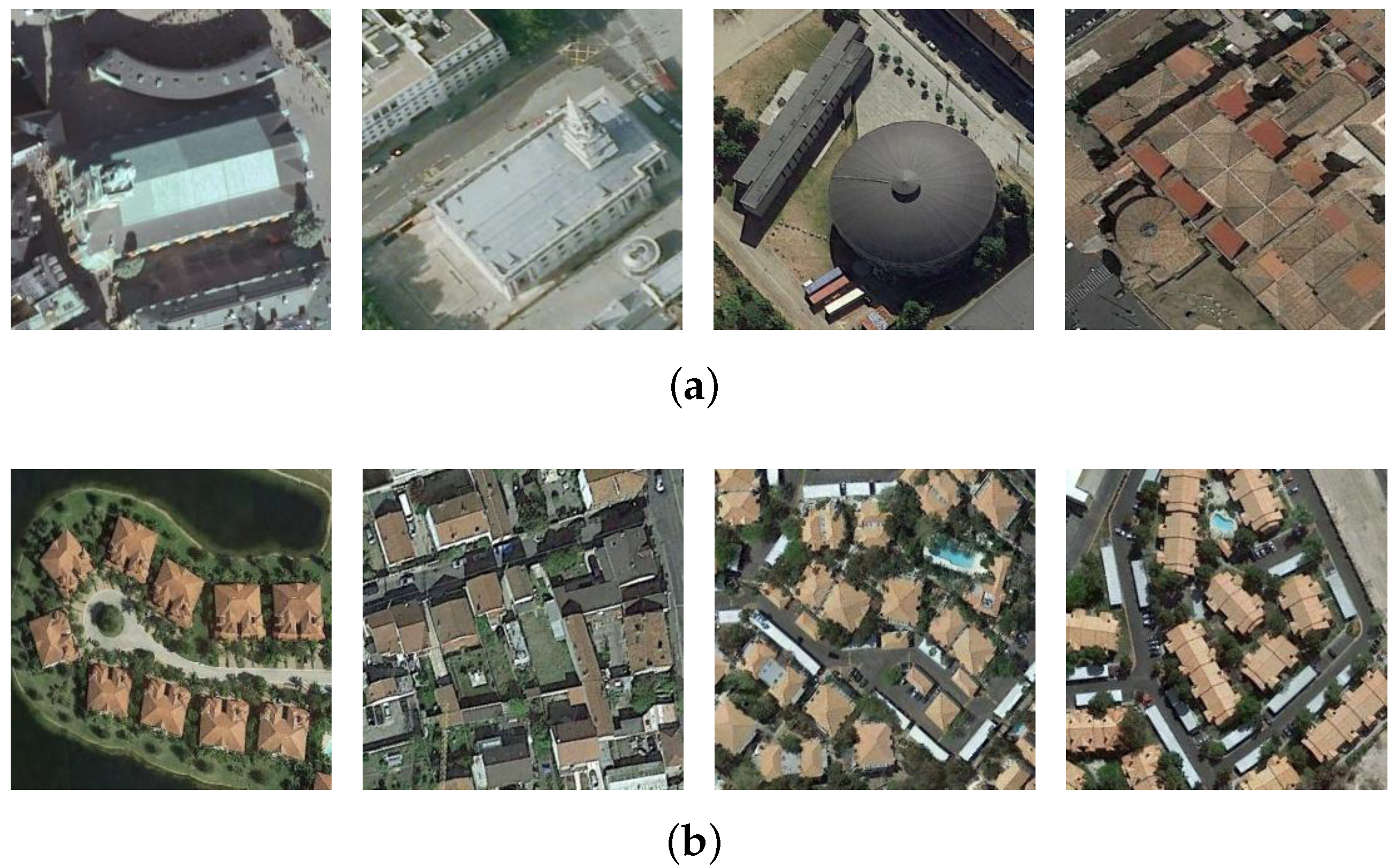
One important characteristic of remote sensing images is that they contain kinds of objects with different poses, shapes, and illuminations, which leads to high intra-class variance in the same object category. As shown in Figure 2a, the four images with very different shapes and layouts are all labelled as a church. Another characteristic states that the images with similar appearances can be labelled as different categories, which causes high inter-class similarity between different categories. As shown in Figure 2b, although the four images have similar views, the left two examples belong to dense residential while the right two belong to medium residential. Therefore, the properties of high inter-class similarity and high intra-class variance pose a great difficulty to remote sensing image scene classification, which is addressed through metric learning in most of the existing methods. For example, Cheng et al. [21] optimized a distance function on the CNN features, such that the distances between the object features in the same category were suppressed, while the distances between the object features in different categories were maximized. Wei et al. [22] proposed an adaptive marginal centre loss function to enhance the contribution of hard samples during the training process.
The above-discussed issues have been tackled by the existing methods which, however, only focused on a certain issue rather than developing a unified pipeline for solving all issues. In this paper, we propose an end-to-end adaptive decision-level fusion framework, which can simultaneously address the issues of information fusion, high inter-class similarity, and high intra-class variance in remote sensing image scene classification. Specifically, the fusion is conducted among the classification scores produced by different layers, meaning that the information with different levels of semantics is fused. In this way, it is not necessary to adjust the dimensions of the classification scores before fusion, nor need to consider the normalization operation for constraining the value range, where hence a natural fusion process is obtained. To implement an adaptive fusion strategy, we propose an importance factor generator that can dynamically assign an importance factor to the corresponding score of each category, which could help to decrease the high inter-class similarity and the high intra-class variance in the score space. To further improve the performance, we develop a stochastic decision-level fusion training strategy that allows each classification score to participate in the decision-level fusion with a certain probability in each training iteration, which is inspired by the idea of Dropout [23]. Experimental results compared with the state-of-the-art methods on four popular remote sensing scene classification datasets demonstrate the superiority of the proposed method. The main contributions of this paper can be summarized as follows:
- We propose an end-to-end adaptive decision-level information fusion strategy, which not only overcomes the problems brought by feature-level fusion, but also solves the issues of high inter-class similarity and high intra-class variance in remote sensing images.
- An importance factor generator is developed to support the decision-level fusion, which can adaptively generate importance factors for different categories in the classification score.
- Through improving Dropout, we propose a stochastic training strategy for the decision-level fusion, which is empirically proved effective.
- Extensive experiments on public datasets illustrate the state-of-the-art performance of our method.
2. Related Work
In this section, we briefly review the related work of remote sensing scene classification. The existing methods with CNN could be divided into three categories: the conventional CNN features-based methods [12,24], the feature-level fusion-based methods [16,17,18,19,20,25,26,27,28,29,30,31,32,33,34], and the decision-level fusion-based methods [35,36].
2.1. The Conventional CNN Features-Based Methods
Among the recent competitive models, CNN has been widely applied in remote sensing image scene classification due to its strong nonlinear representation ability. Early applications of CNN employed simple convolutional architectures to classify remote sensing images directly. For example, Dimitrios et al. [24] applied the model pretrained on ImageNet to the task of remote sensing image scene classification, which alleviated the problem of limited training samples in remote sensing datasets. Cheng et al. [12] used the pretrained model to extract features which were then classified by linear SVM. This method also empirically verified the effectiveness of model fine-tuning via transfer learning. Compared with the handcrafted feature-based methods, these deep learning-based methods have achieved a great improvement in classification performance.
2.2. The Feature-Level Fusion-Based Methods
To improve the discriminativity of deep features, information fusion has been integrated into the elaborated CNN architectures. Feature-level fusion is a typical option for information fusion in remote sensing scene classification. Zhang et al. [25] proposed an efficient multi-network integration method for the first time through parameter sharing, resulting in significant improvement of the classification performance compared with a single network. Zhang et al. [27] combined the features extracted from VGG-16 and Inception V3, which were then fed into the capsule network to obtain better classification results. Muhammet et al. [28] proposed a network integration strategy based on Snapshot and Homogeneous, which only fused the information of the last convolutional layer of each network, overcoming the problem of costly computation in multi-network integration. These feature-level fusion strategies based on multiple networks could yield pleasing classification performance, but bring heavy computation cost, hence being inefficient.
Other forms of feature-fusion are also common in remote sensing image scene classification. Fang et al. [18] explored the features of remote sensing images in the frequency domain, which were fused with the spatial-domain features to obtain better robustness. Dong et al. [16] fused the deep CNN features with the GIST features before the classification by LSTM. Xu et al. [17] proposed a two-stream feature fusion method, where one stream provided features using a pretrained CNN while the other output the multi-scale unsupervised MNBOVW features. Shi et al. [19] proposed a network with several groups, each of which had two branches for feature extraction and fusion respectively. Xu et al. [20] fused four groups of intermediate feature maps of the network through pooling, transformation, and other operations, to encourage efficient adoption among multi-layer features. Lu et al. [30] claimed that the label information was crucial to the effect of feature fusion, and proposed to supervise the softmax outputs of the fused features by semantic labels.
In remote sensing scene classification, the semantic features of an image may be closely correlated with local regions, which suggests that different regions in a remote sensing image are of different importance for accurate classification. However, the above-reviewed methods ignore this fact. To solve this problem, Sun et al. [31] proposed a gating mechanism, allowing the network to determine which area is suitable to be fused. Based on the attention mechanism, Ji et al. [32] drove the network to focus on the features of the most attractive regions in an image such that redundant features could be removed and the classification performance was then improved. Yu et al. [33] adopted ResNet-50 to extract features which were then adaptively enhanced by a channel attention module and finally fused by bilinear pooling. Zhang et al. [34] proposed a location-context fusion module, which could not only distinguish different regions but also met the translation invariance that was very helpful for image scene classification.
2.3. The Decision-Level Fusion-Based Methods
In addition to model fusion and feature fusion, the decision-level information fusion methods have also been applied in remote sensing scene classification. Li et al. [35] used a CNN model to get the top-N categories, and then input the features extracted by the dual networks into SVM to obtain the final category. The method involves multi-step operations and does not provide end-to-end training. Wang et al. [36] proposed a dual-stream architecture, in which one stream used the SKAL strategy to extract features of interested areas while the other stream extracted the global features. These features were respectively classified, the results being averaged to get the final score. Note that the fusion strategy in this method was rough since there was no difference between the contributions of the local features and the global features. In our work, the proposed architecture solves the problem of contribution allocation and adaptive decision-level fusion simultaneously.
3. The Proposed Method
In this section, we first illustrate the overall framework of the proposed method and then introduce the importance factor generator and the adaptive decision-level fusion method in detail. Finally, the stochastic decision-level fusion training strategy is presented.
3.1. Framework
Most of the existing CNN models have a typical architecture that can be divided into the feature extraction backbone and the classification head. The feature extraction backbone involves a hierarchical structure that tends to extract the semantics of different levels through subsampling or pooling in different depths. We could regard the layers between adjacent subsampling or pooling layers as a stage. To be explicit, the width and the height of the feature maps in all layers of a stage are consistent. As is well known, the features in shallow stages have low-level semantics while the deep stages provide high-level semantics.
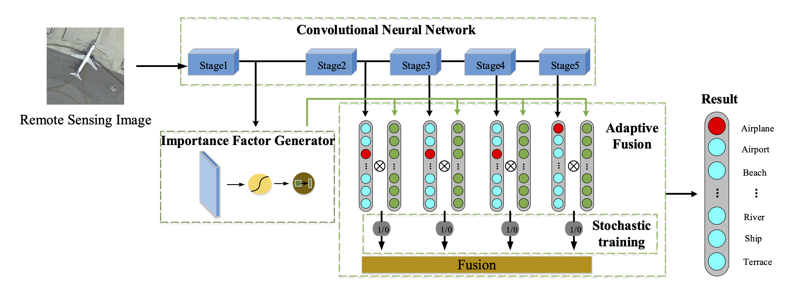
The proposed framework aims at exploiting the discriminativity of the features in different stages. As shown in Figure 3, we group the stages of the CNN backbone as stages (where in the figure). In each of the last n stages, the sizes of the feature maps of all layers keep consistent. The first stage contains all the remained shallow layers, where the sizes of the feature maps may vary. The outputs of the last n stages are employed for classification, where each output produces a classification score. The output of the first stage is fed into the importance factor generator for generating the importance factors (s). These important factors diversify the importance of each category in the classification scores as well as the importance of different stages. Specifically, the importance factor generator generates n factors with each having the same dimension as the classes of the interested task. The n factors correspond to the last n stages. The values of the factors range from 0 to 1, hence being viewed as weights for the classification scores. The n factors and the n classification score vectors are element-wisely multiplied, followed by a class-wise summation of all the processed score vectors. Finally, a fused classification score vector is obtained. Note that the importance factors produced by the importance factor generator are determined by the input image, or specifically its shallow features, which means that the decision-level fusion process can be adjusted adaptively.
3.2. Importance Factor Generator
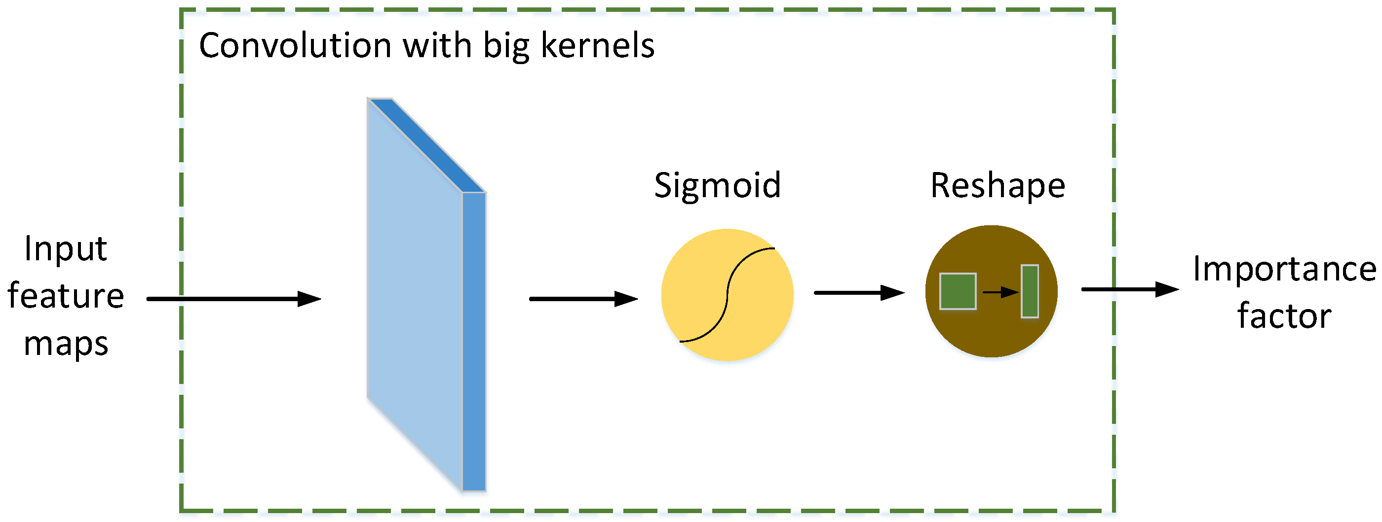
The function of the importance factor generator is to process the feature maps produced by the first stage and generate an importance factor matrix to adaptively fuse the classification scores. For example, for an N-classification problem, the importance factor generator produces an importance factor matrix with the size of . As shown in Figure 4, the implementation is to pass the feature maps of the first stage through a convolutional layer with big kernels where the kernel size is related to the size of the feature maps and the number of the categories in the task. The following is the sigmoid activation layer and the dimension reshape layer. Mathematically, the importance factor matrix A can be written as:
where is the feature maps of the first stage, and are the weight and bias of the convolutional layer, respectively, and is the sigmoid function.
3.3. Adaptive Decision-Level Fusion
In the fusion process, the classifier of each stage is composed of a global pooling layer, a convolutional layer, and a softmax layer. The global pooling layer is implemented as average pooling, i.e., averaging all pixels along the width and height dimensions of the feature maps. The global pooling is robust to the spatial translation of the input image.
Concretely, the output feature maps of the stage which have a size of are passed through the global average pooling layer, resulting in a tensor with a size of . We denote as the element in column j and row k of the feature maps of the stage. Then,
The tensor is then processed by convolution which transforms the channel dimension from to the number of categories N, and then followed by the softmax layer to get the corresponding classification score , i.e.,
where and are the weight and bias of the convolutional layer for the stage.
Once the importance factor matrix and the classification scores are obtained, the decisions are fused as follows. As shown in Figure 3, we first multiply each classification score vector (i.e., ) with the corresponding importance factor by elements, which produces a weighted classification score. Then, the weighted scores of all stages are summed up to complete the decision-level fusion. Finally, the softmax layer is adopted to convert the fused score to the final classification result Y. The above fusion process can be expressed as
where , v is a n-dimensional vector full of 1 and ⊙ is element-wise multiplication.
This decision-level fusion method not only realizes the fusion of hierarchical information, but also alleviates the problem caused by high inter-class similarity and high intra-class variance in remote sensing images, which are discussed in the following.
- (1)
- Discussion on reduction of intra-class variance
The intra-class variance refers to the difference between the images belonging to the same category. In remote sensing image scene classification, the images generally exhibit high intra-class variance in which case the deep model predicts diverse scores on the ground-truth class for different images of the same category, hence posing a great difficulty for classification.
Let denotes score of the category in the stage and be the adaptively fused classification score of the category which can be expressed as
where g represents the softmax operation to normalize the scores.
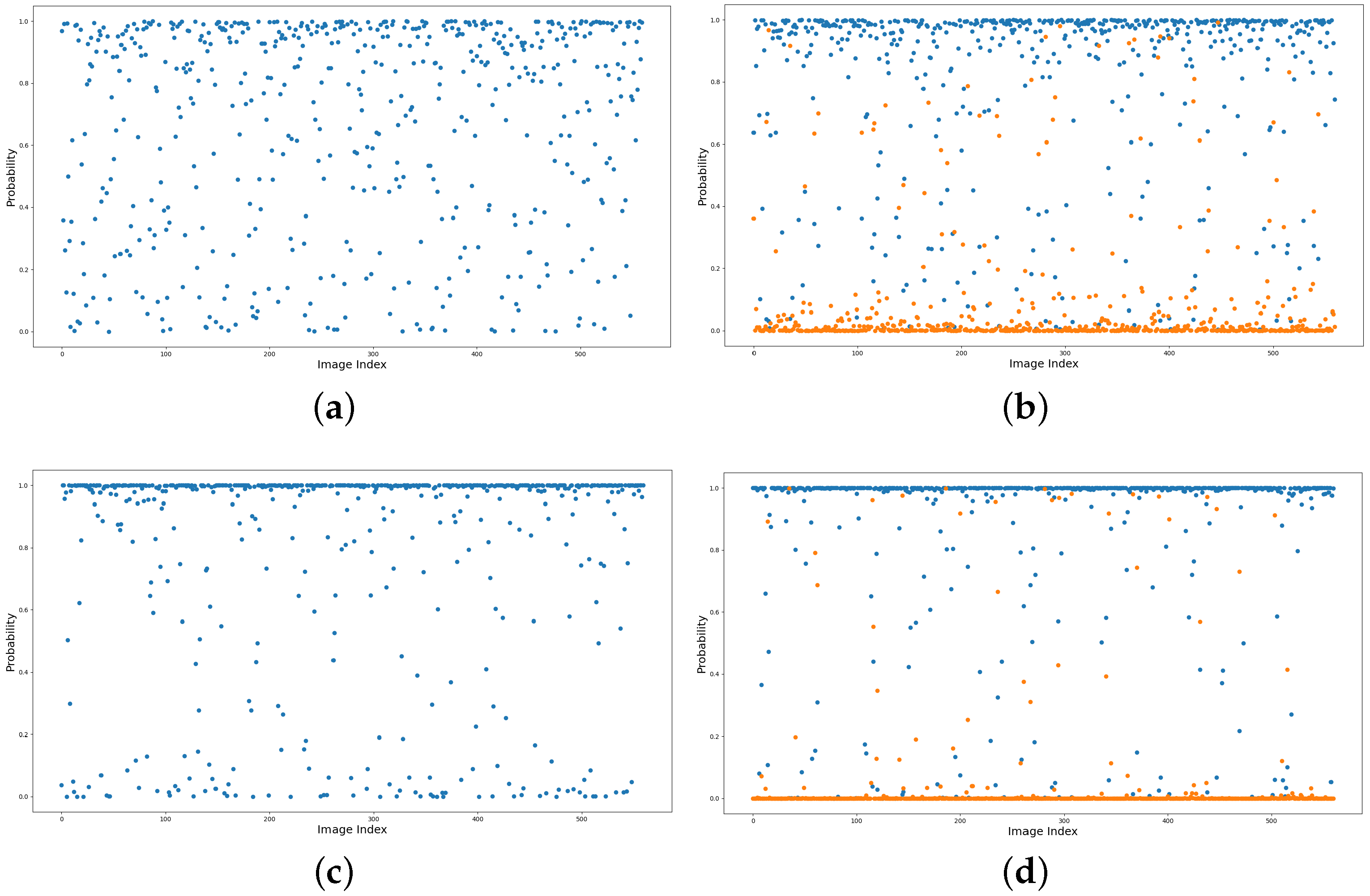
The existing studies show that the discrimination ability of the feature representation in a single layer of a deep CNN model is insufficient for accurate classification, mainly because of the complex scene conditions (e.g., diverse shapes, illuminations, and textures). As shown in Figure 5a, the output score of ResNet-50 varies diversely for different images of the same class, in this case church. Instead, by taking the importance factor into consideration, the model tends to generate high factors for the important features while suppressing the useless features, which can yield a more accurate result as shown in Figure 5c.
- (2)
- Discussion on reduction of inter-class similarity
Inter-class similarity refers to the similarity between the images belonging to different categories. In remote sensing image scene classification, the deep model could predict similar scores on a certain category for two images of different classes; generally, the category is the ground-truth label for one of the two images.
Let and denote the stage scores of the and categories, respectively. The distance which can be expressed below will be small if these two classes have high inter-class similarity:
Let and be the adaptively fused classification score of the and categories, respectively. According to Equation (5), the distance between and can be written as:
Similarly, a single layer of a deep model is insufficient to predict reliably for these classes. As shown in Figure 5b, the output scores of dense residential and medium residential are partially mixed, indicating that the boundary between these two classes is not clear enough. After the adaptive fusion, the importance factors help to produce high scores for the interested classes. It is seen from Figure 5d that the score margin between the two classes become clearer than the case without score fusion. This also indicates the validity of the proposed fusion strategy.
3.4. Stochastic Decision-Level Fusion Training Strategy
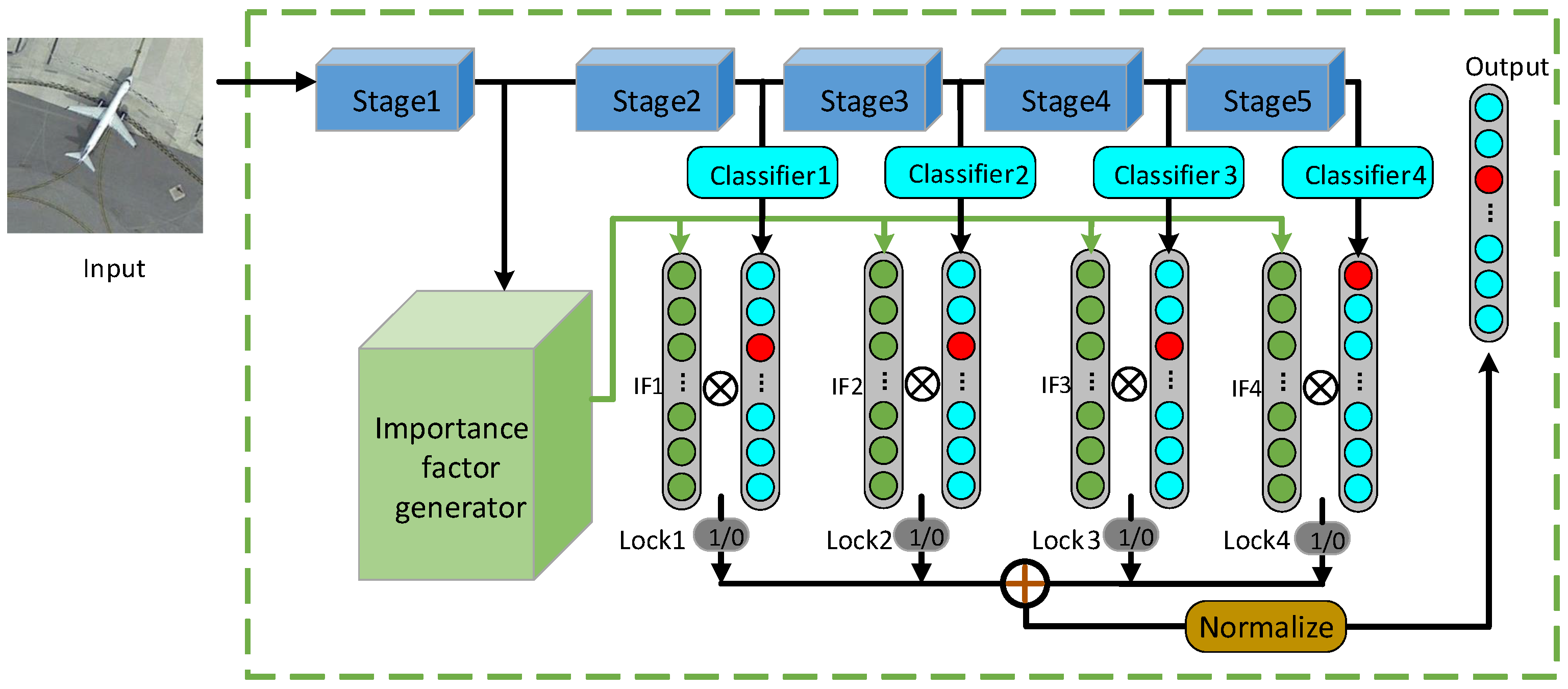
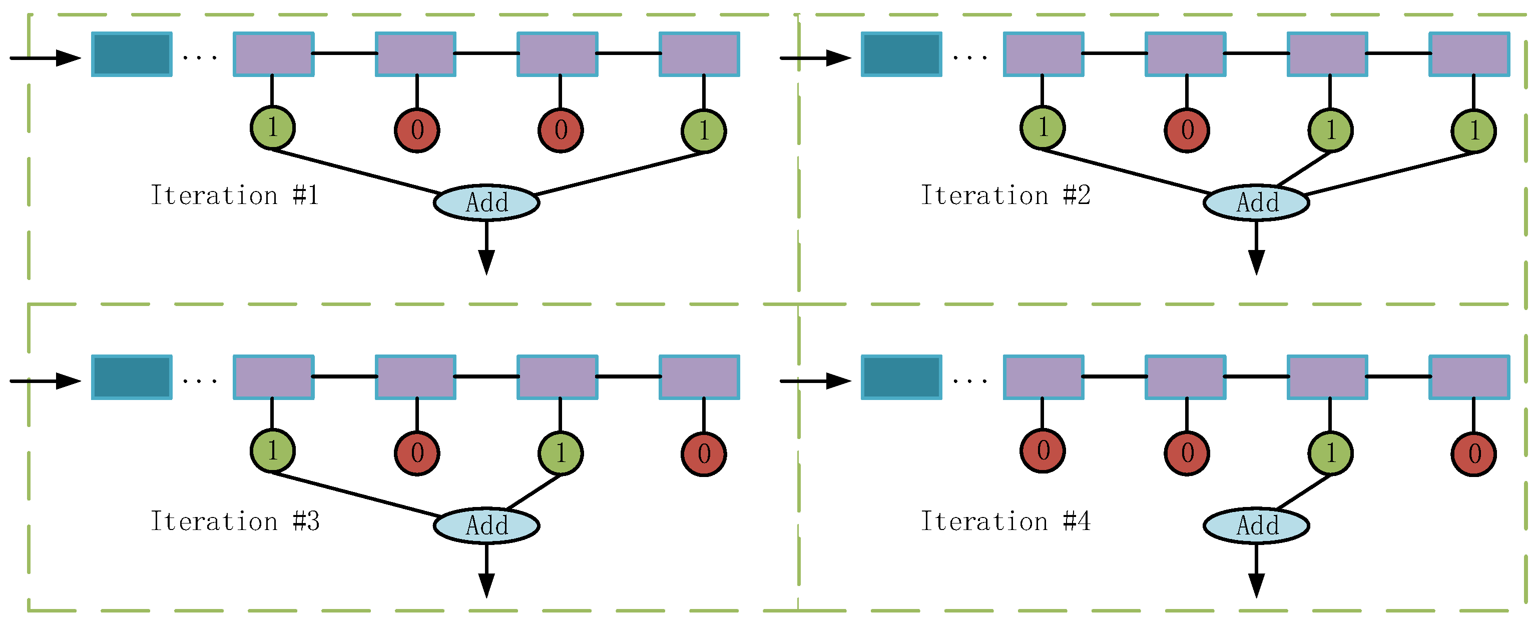
Dropout informs us that during the training process, by ignoring a neuron with a certain probability, this neuron would be independent from other neurons of the same layer, and this operation can reduce the co-adaptation between different neurons and enhance the representation ability of each neuron. This idea drives us to propose a stochastic decision-level fusion training strategy. As shown in Figure 6, in each training iteration, the classifiers will stochastically participate in the adaptive decision-level fusion process with a certain probability which is called survival rate.
Specifically, we set the same initial survival rate for all classifiers, which is fixed for the first epochs of training. Then, the survival rate is increased gradually in a sinusoidal way as the training goes on to improve the stability of the training process. We use to denote the survival rate at the epoch, which can be expressed as
where T is the total training epochs.
In this way, each classifier could participate in the final decision process with a certain probability. The optimization encourages that different classifiers are independent from each other, where each tends to produce an accurate result. Hence, the stochastic training strategy improves the performance of the fused decision.
4. Experiments
In this section, we present the details of the experiments to validate the effectiveness of the proposed framework.
4.1. Datasets
We employ four public and popular datasets for remote sensing scene classification, which are introduced as follows.
- UC Merced Land-Use Dataset (UCM) [37]: This dataset is collected from the USGS National Map Urban Area Image series. The dataset contains 2100 scene images of 21 categories, including 100 images for each category. The image resolution is , and the spatial resolution of each pixel is 1 foot. In the experiment, we randomly choose 50% and 80% of the samples as the training set, and the rest is the test set.
- RSSCN 7 Dataset [38]: This dataset contains 2800 remote sensing images from 7 typical scene categories including grassland, forest, farmland, parking lot, residential area, industrial area, river, and lake. Each category contains 400 images. The resolution of each image in this dataset is . These images are photographed in different seasons and weathers, and sampled in different proportions, thus making the scenes very diverse and challenging. In the experiment, 50% of the samples are randomly selected as the training set, while the rest is regarded as the test set.
- Aerial Image Dataset (AID) [39]: It is collected from Google Earth, which contains 10000 images of 30 categories, where each category has about 220 to 420 images. Each image has a resolution of . The images are collected in different locations, weathers, and other conditions, hence posing the challenge of high inter-class similarity. In the experiment, we randomly take 20% and 50% of the samples as the training set, and the rest is the test set.
- NWPU-RESISC 45 Dataset (NWPU 45) [1]: It contains 31,500 remote sensing images with the resolution of , belonging to 45 scene categories with each consisting of 700 images. The dataset has the properties of high inter-class similarity and high intra-class variance. In the experiment, we randomly select 10% and 20% of the samples as the training set and keep the rest as the test set.
4.2. Evaluation Metrics
To make a quantitative comparison, we adopt the widely used overall accuracy and the confusion matrix to evaluate the performance of all the competitors.
- The overall accuracy (OA) is obtained by dividing the number of correctly classified images by the number of all images in the test set, which demonstrates the overall classification performance of the model.
- The confusion matrix (CM) is a matrix where N is the number of categories. The value at the row and the column indicates the proportion of the samples in class i being predicted as class j. The confusion matrix clearly shows which two categories are difficult to be distinguished from each other.
4.3. Experimental Settings
All experiments are carried out by using the open-source deep-learning library Pytorch. Unless noted otherwise, we adopt ResNet-50 [40] as the backbone to examine the performance of the proposed framework. The pre-trained weights of ResNet-50 on ImageNet are employed as the initialization of the model parameters, which are then fine-tuned on the corresponding dataset. In the RSSCN 7 and AID datasets, we resize the images to . While the input size of the model is set to , all images with the size of are randomly cropped to . The batch size is set to 32 and the number of training epochs is set to 200. SGD optimizer is employed while the momentum is set to 0.9 and the regularization coefficient is set to 0.0005. The initial learning rate is 0.001, which is then adjusted according to the cosine annealing strategy. In addition, we use the data augmentation options to enhance the generalization performance of the model, such as random horizontal flip, vertical flip, and 90° rotation. All the implementations are conducted on the Ubuntu 16.04 operating system equipped with a 3.3 GHz CORE i9-7900x CPU and two NVIDIA 2080Ti GPUs.
4.4. Ablation Study
- (1)
- Investigation on model size and efficiency
The proposed importance factor generator involves very limited parameters but brings a noticeable improvement in performance. To validate this, we first examine how the model size and FLOPs change when the backbone is equipped with the decision-level fusion plugin. The model size is measured using the number of parameters. Considering that the execution time of the model on different devices is different, FLOPs instead of latency is used to represent the model efficiency. The results are shown in Table 1 and Table 2. It is seen that the improved model has a very limited increase in the number of parameters and FLOPs compared with the original ResNet-50. The differences across the datasets are caused by the different numbers of categories.
- (2)
- Investigation on different backbones
The proposed importance factor generator is the key to improve the performance of the deep models. To validate the effectiveness of this plugin, we employ multiple backbones including VGG-16, MobileNet V2, ResNet-50, and ResNet-152. The RSSCN 7 dataset is used with a training ratio of 50%. The survival rate is set to 0.8 for VGG-16 and 0.9 for MobileNet V2 and ResNet-152, respectively. As seen from Table 3, compared with the original models, the accuracies are improved by 1.75%, 1.72%, 2.86%, and 3.73%, respectively. Moreover, the stochastic decision-level fusion training strategy further increases the accuracies by 0.38%, 0.98%, 0.34%, and 0.67%, respectively, which demonstrates the effectiveness. It is known that MobileNet V2 is a popular lightweight model which is opposite to VGG-16 that has 138 MB parameters. Hence, this indicates that our method works well with models of different sizes.
- (3)
- Investigation on survival rate
To examine how the proposed stochastic training strategy performs, here we conduct experiments with different survival rates and compare the corresponding classification performance. The AID dataset is employed in the case of 50% training samples. The candidate survival rate ranges from 0.4 to 1 and the same value is set for each classifier. To reduce the deviation, the experiment in each case is conducted ten times, and the averaged performance is used for comparison.
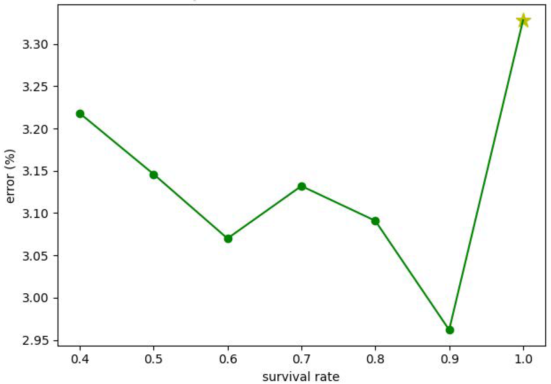
Figure 7 illustrates the error rate under different survival rates, in which the yellow star (i.e., the survival rate is 1.0) corresponds to the performance of the model trained without the stochastic decision-level fusion training strategy. It is clearly seen that the stochastic training strategy can improve the classification accuracy. According to the rationale of Dropout, we understand that the stochastic training strategy reduces the co-adaptation effect between different classifiers and hence the performance is improved. We also note that when the survival rate is reduced smaller than 0.9, the accuracy gradually decreases. This is because when the survival rate is too small, the error is difficult to be backpropagated, affecting the optimization of model parameters.
From the viewpoint of optimization, a good optimization method possesses a good balance between the global exploration capability and the local exploitation capability. The purpose of global exploration is to explore as large areas as possible in the solution space, while local exploitation is to exploit the fine structures of the known areas to obtain a better solution. In our method, by randomly ignoring the classification results during fusion, the proposed strategy could diversify the solution space, which corresponds to the global exploration. When the global structure of the solution space has been explored sufficiently, the fine-tuning process means exploiting the fine structures. Therefore, the stochastic decision-level fusion training strategy can be regarded as a trade-off between global exploration and local exploitation.
In subsequent experiments, we set different survival rates for different datasets and different training-test split ratios. Generally, the datasets with a large number of samples need global exploration, whereas the datasets with limited samples require local exploitation. The survival rates for different cases are listed in Table 4.
4.5. Comparison with State-of-the-Art Methods
We compare the proposed method with the state-of-the-art methods on the four datasets. To reduce the deviation, the experiment in each case is conducted ten times, and the averaged result is used for comparison.
- Experimental results for the UC Merced Land-Use dataset
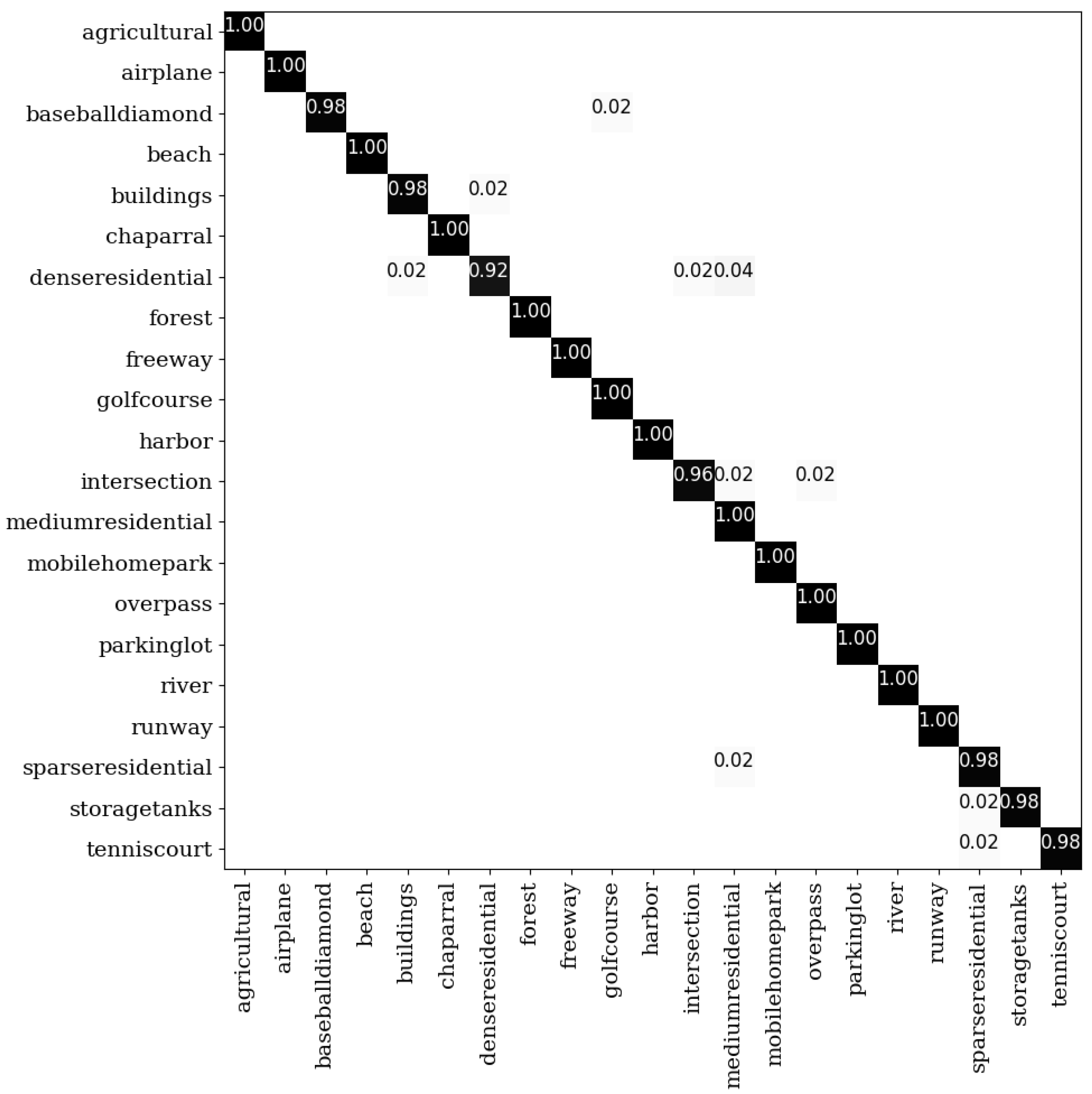
The comparison with the state-of-the-art methods for the UC Merced land-use dataset is shown in Table 5. The classification accuracies of the proposed method in the cases of both 50% and 80% training samples are 98.65% and 99.71%, respectively, which surpass most of the competitors. ADFF [43] and ResNet_LGFFE [44] are based on feature-level fusion, and their backbones are both ResNet-50. In the case of 50% training samples, the accuracy of our method is 1.43% higher than that of ADFF; in the case of 80% training samples, the accuracy of our method is increased by 0.9% and 1.09% compared with ADFF and ResNet_LGFFE, respectively. This shows the superiority of the adaptive decision-level fusion in our method. With the stochastic decision-level fusion training strategy, the accuracy under 50% training samples is improved by 0.25%, while the accuracy under 80% training samples is slightly reduced. The main reason is that the performance under 80% training samples nearly reaches the perfect, which is difficult to improve.
The confusion matrix in Figure 8 shows the detailed classification result of each category when 50% samples are used for training. As shown, the accuracies of all categories are above 92%, or even close to 100%. As mentioned above, dense residential and medium residential have high inter-class similarity, which leads to a great challenge. Clearly, our method achieves 92% and 100% accuracies for both scenes, which validates the effectiveness of the adaptive decision-level fusion on reducing the inter-class similarity.
- Experimental results for the RSSCN 7 dataset
Table 6 shows the comparison for the RSSCN 7 dataset. Under 50% training samples, the classification accuracy of our method reaches 95.15%, which surpasses all the competitors including the basic ResNet-50. ADFF [43] achieves the second highest accuracy in the table where the backbone is also ResNet-50 and SVM is adopted for classification. With end-to-end learning, the accuracy of our method is even higher. With the stochastic decision-level fusion training strategy, the performance is further improved by 0.34% and is also more stable.
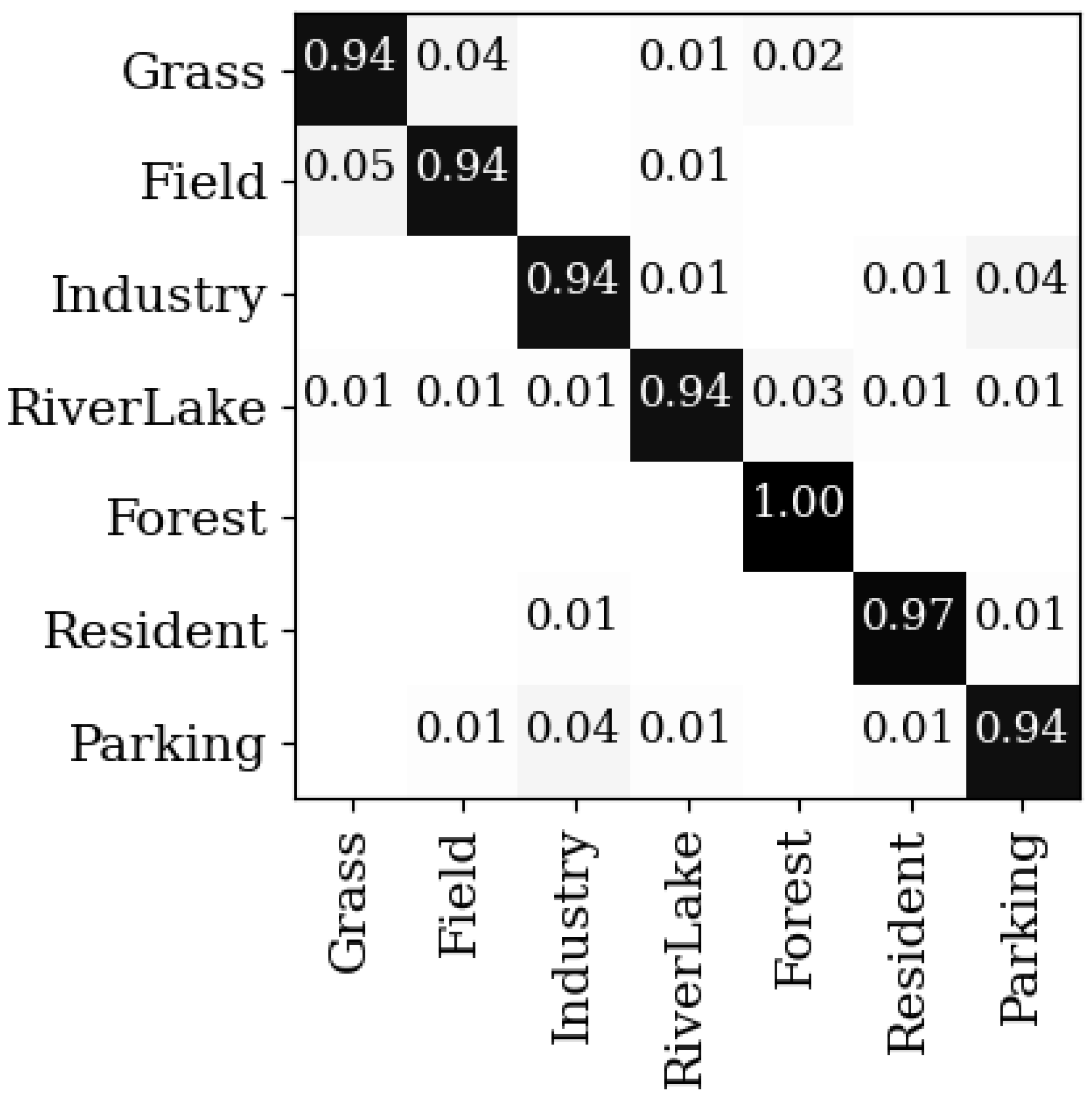
Figure 9 shows the confusion matrix on the RSSCN 7 dataset. The grass class and the field class have high inter-class similarity, and hence low classification accuracies. By contrast, the classification accuracies of ResNet-50 in the grass class and the field class are 85% and 88% which are surpassed by 9% and 6%, respectively [42]. This comparison validates that the proposed method is effective in reducing the inter-class similarity and the intra-class variance.
- Experimental results for the AID dataset
The comparison for the AID dataset is listed in Table 7. It can be seen that there is a clear gap between the proposed method and the other competitors. Our performance reaches 94.69% and 96.67% when the training samples are 20% and 50%, respectively, which are 8.21% and 7.45% higher than ResNet-50. Moreover, the stochastic decision-level fusion training strategy further improves the results by 0.36% and 0.37%.
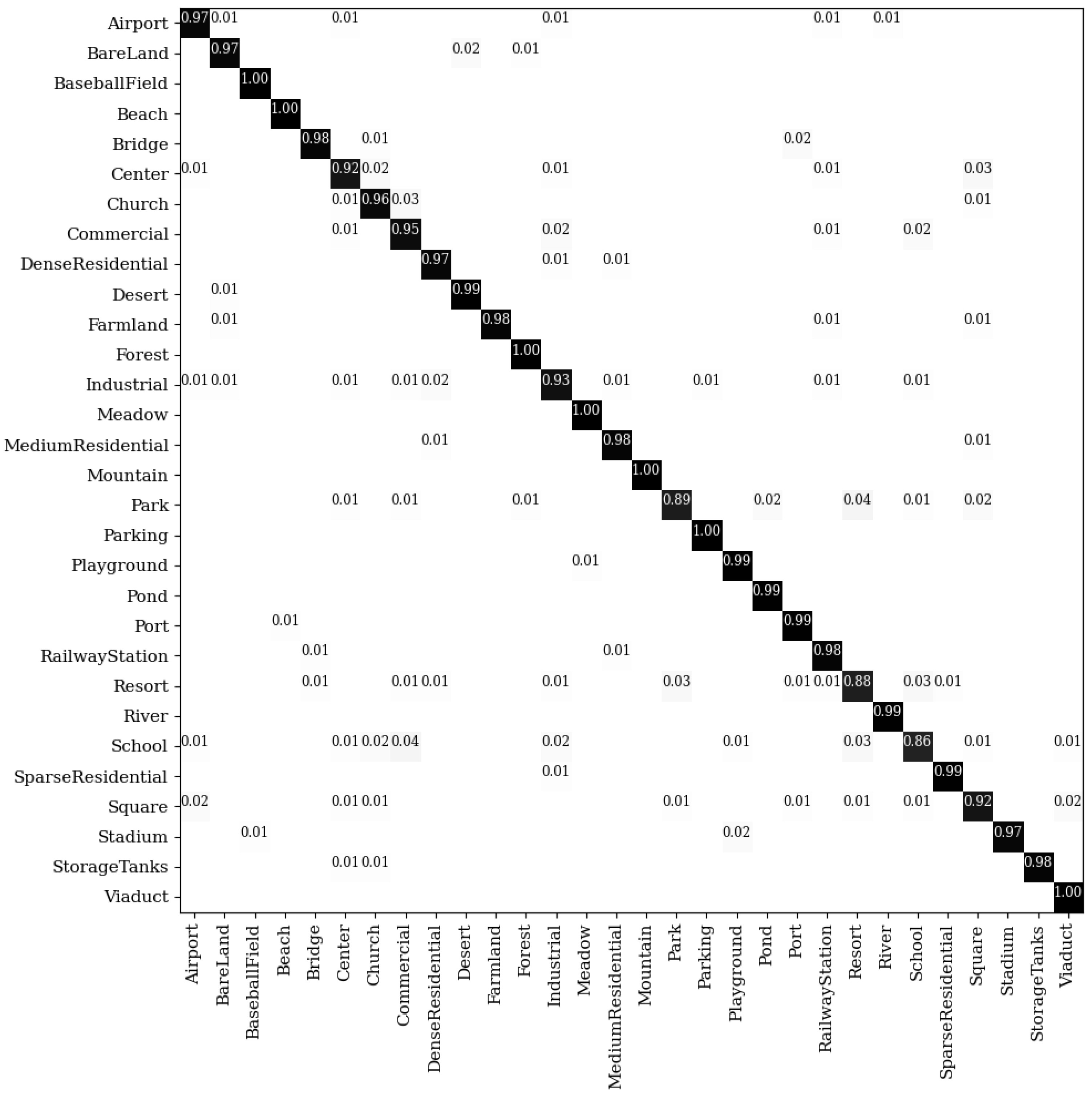
Figure 10 shows the detailed accuracy of each category when the training sample is 50%. Except for the school class and the resort class, the accuracies of other categories are higher than 90%. The resort class has a high similarity relative to other classes such as square, so the classification accuracy is low. Compared with ResNet_LGFFE [44] which adopts ResNet-50 as the backbone, the accuracies on the school class and the resort class are improved by 56% and 28%, respectively. In addition, the accuracies of our method on dense residential areas and medium residential areas are 97% and 98%, respectively, which shows that our method greatly reduces the similarity between these two classes.
- Experimental results for the NWPU-RESISC 45 dataset
Table 8 shows the comparison for the NWPU-RESISC 45 dataset. This dataset is the largest dataset in the remote sensing image scene classification at present. The proportion of the training set is usually low, posing the request of high generalization ability by the model. As seen, the proposed method surpasses most of the other methods. Our accuracy is similar to that of RIR [49] under 10% training samples and is better than RIR in the case of 20% training samples. Similar effects with the stochastic decision-level fusion training strategy are again observed.
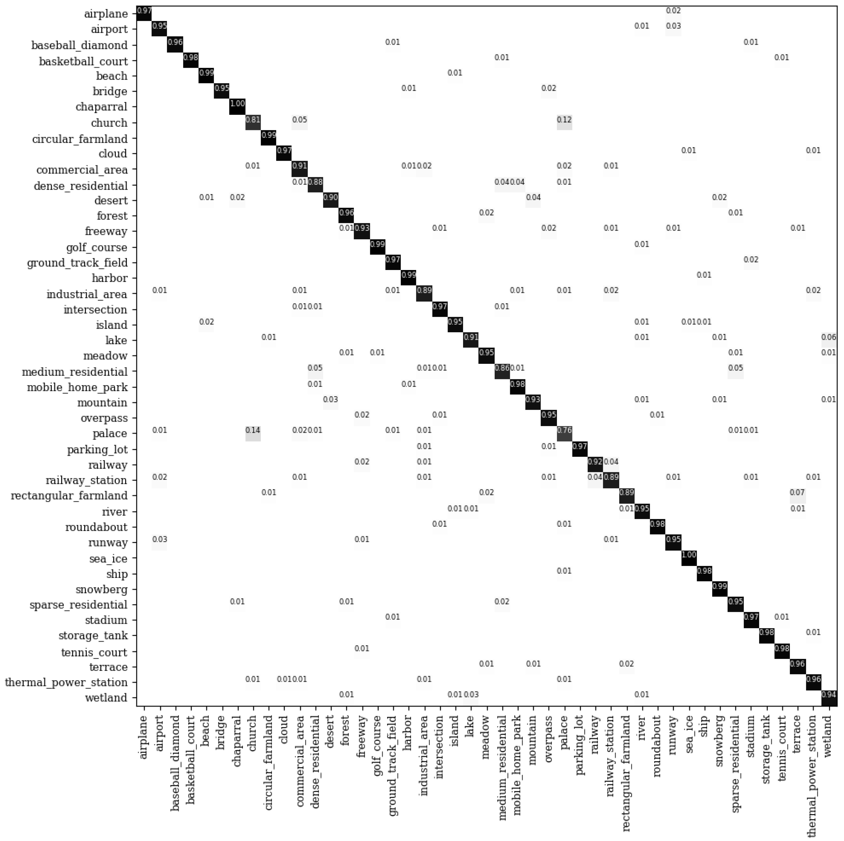
Figure 11 shows the confusion matrix in the NWPU-RESISC 45 dataset. It is observed that our method performs well in all categories except for those with great intra-class variance and inter-class similarity such as church, palace, and commercial area. However, compared with DCNN [21] which focuses on inter-class similarity and intra-class variance, the accuracies of our method in the commercial area and palace classes are still increased by 6% and 3%, respectively, which further verifies the superiority of our method in reducing intra-class variance and inter-class similarity.
4.6. Analysis about the Fusion Strategy
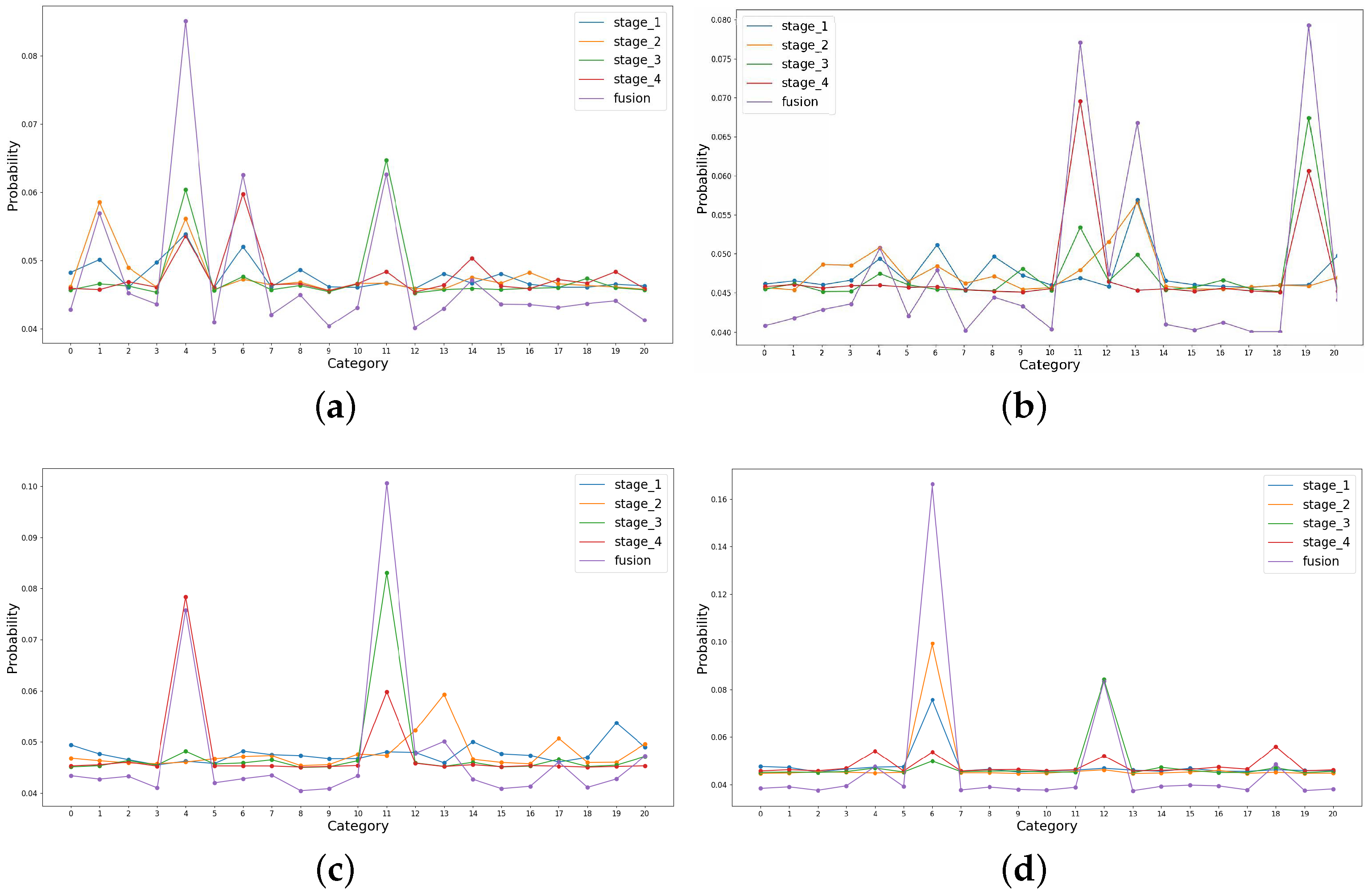
Through extensive experiments, our proposed adaptive decision-level fusion based-method has shown superior performance. Here, we detail the varied scores before and after the fusion process. Specifically, we randomly select four examples that belong to #4 (buildings), #19 (storage tanks), #11 (intersection), and #6 (dense residential), respectively, from the UC Merced Land-Use dataset. The output scores of different stages are shown in Figure 12.
As seen, the output scores vary significantly in different stages. For example, in Figure 12a, the predicted classes in the four stages are #4 (buildings), #1 (airplane), #11 (intersection), and #6 (dense residential), respectively, while the fused probability results in the correct prediction. Considering that different stages of the deep CNN model may produce different classes, the average fusion or the max fusion strategy is also applicable but not necessarily effective. For example, if we regard the max score in Figure 12b, the image is mistakenly classified as #11 (intersection). Instead, the proposed importance factor generator can predict the weights adaptively according to the image itself, encouraging proper supervision during the model training. In other words, our method can be viewed as a generalization of the conventional decision-level fusion strategies, which possess high adaptivity to the image content and hence, can improve the fault tolerance of the model.
5. Discussion
In this section, we present a detailed discussion on how the proposed information fusion strategy alleviates the issues caused by the loss of small objects, high inter-class similarity, and high intra-class variance. Specifically, the discussion starts from the comparison of different layers between the original ResNet-50 and the proposed method. All test examples are selected from the NWPU-RESISC 45 dataset.
5.1. Avoiding the Loss of Small Objects
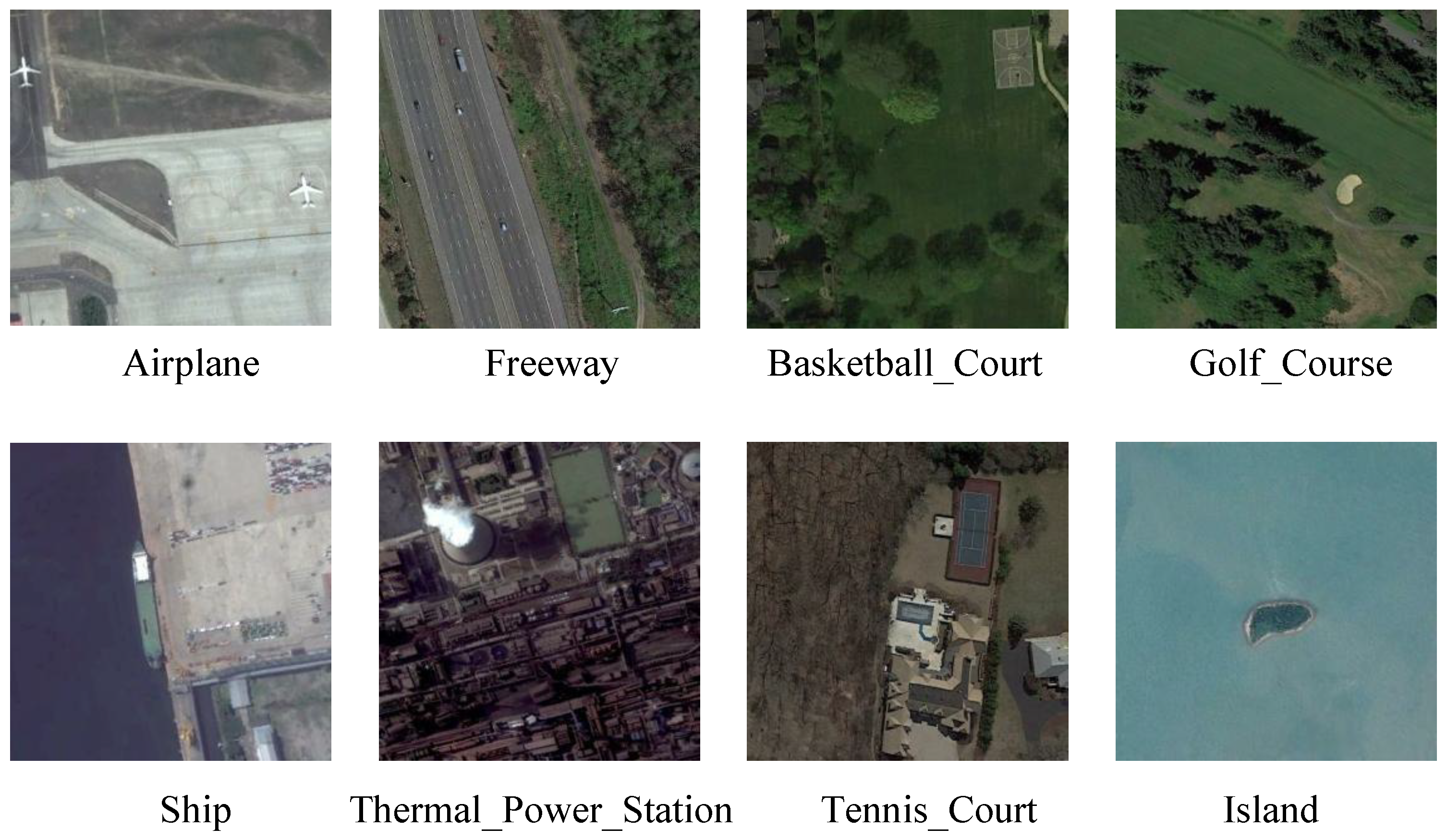
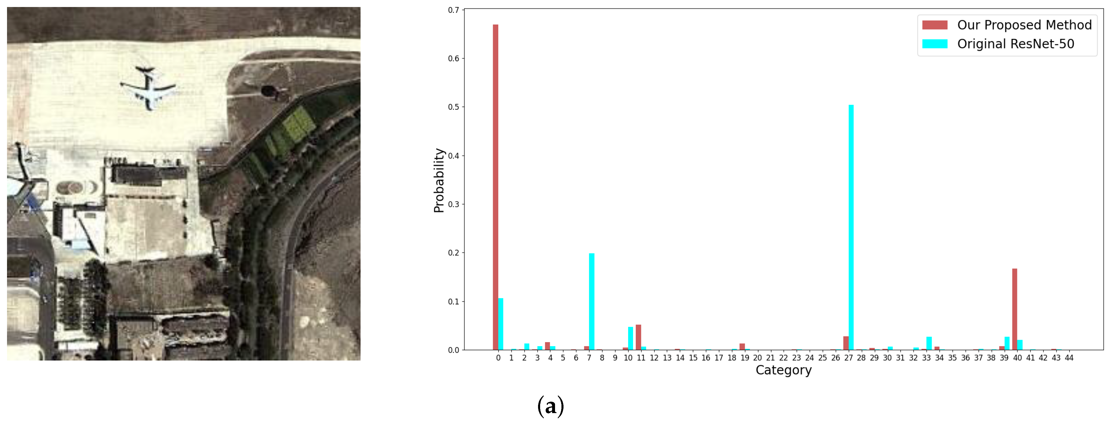
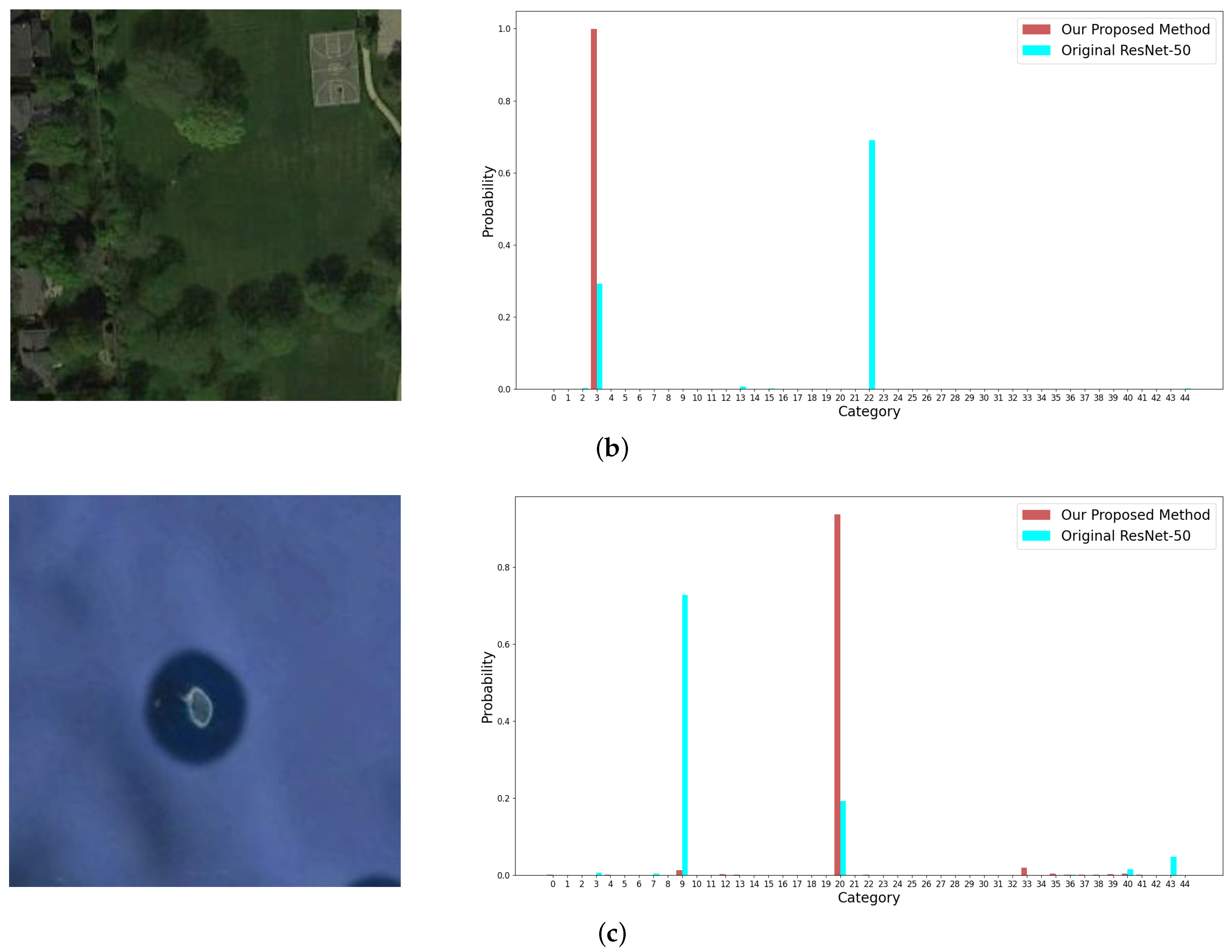
It is common in remote sensing datasets that objects occupying small areas are usually discriminative to classify the images. As shown in Figure 13, three remote sensing images with small objects, which are labelled as airplane, basketball court, and island, respectively, are used to validate that the proposed fusion strategy can avoid the loss of small objects in feature extraction and hence, improve the performance.
The images are misclassified as #27 (palace), #22 (meadow), and #9 (cloud), respectively, by ResNet-50, which only pays attention to the background and ignores the small objects in deep CNN layers. By contrast, our method fuses the information from the shallow layers to the deep layers adaptively, which preserves the features of small objects in the final feature representation, thus correcting the classification results.
5.2. Reducing the Inter-Class Similarity and Intra-Class Variance
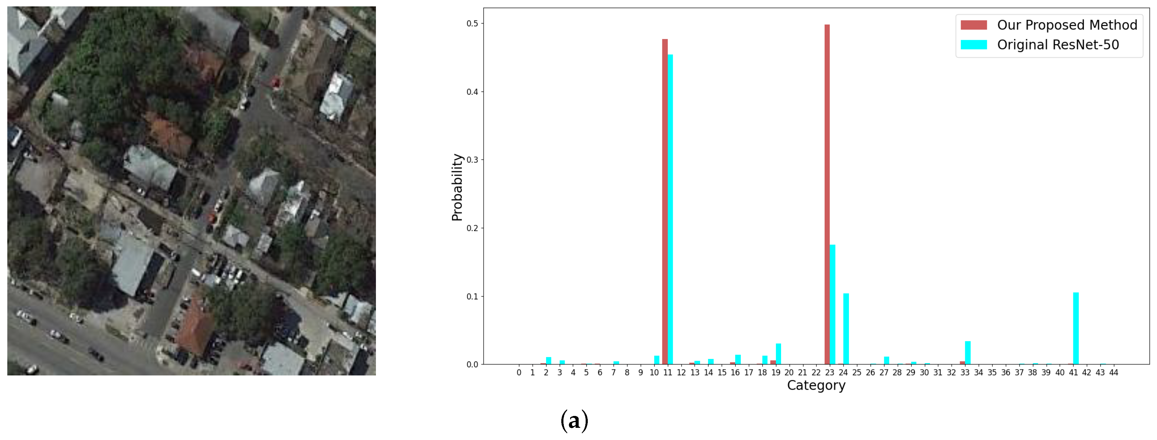
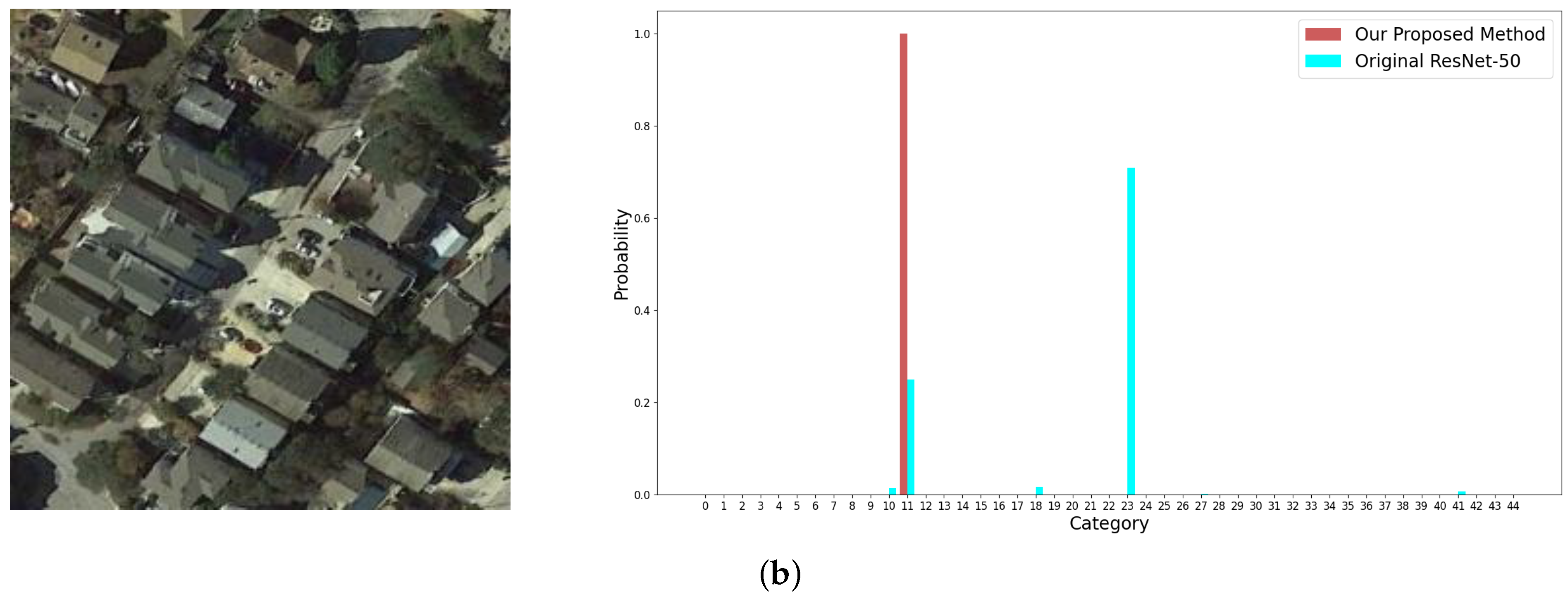
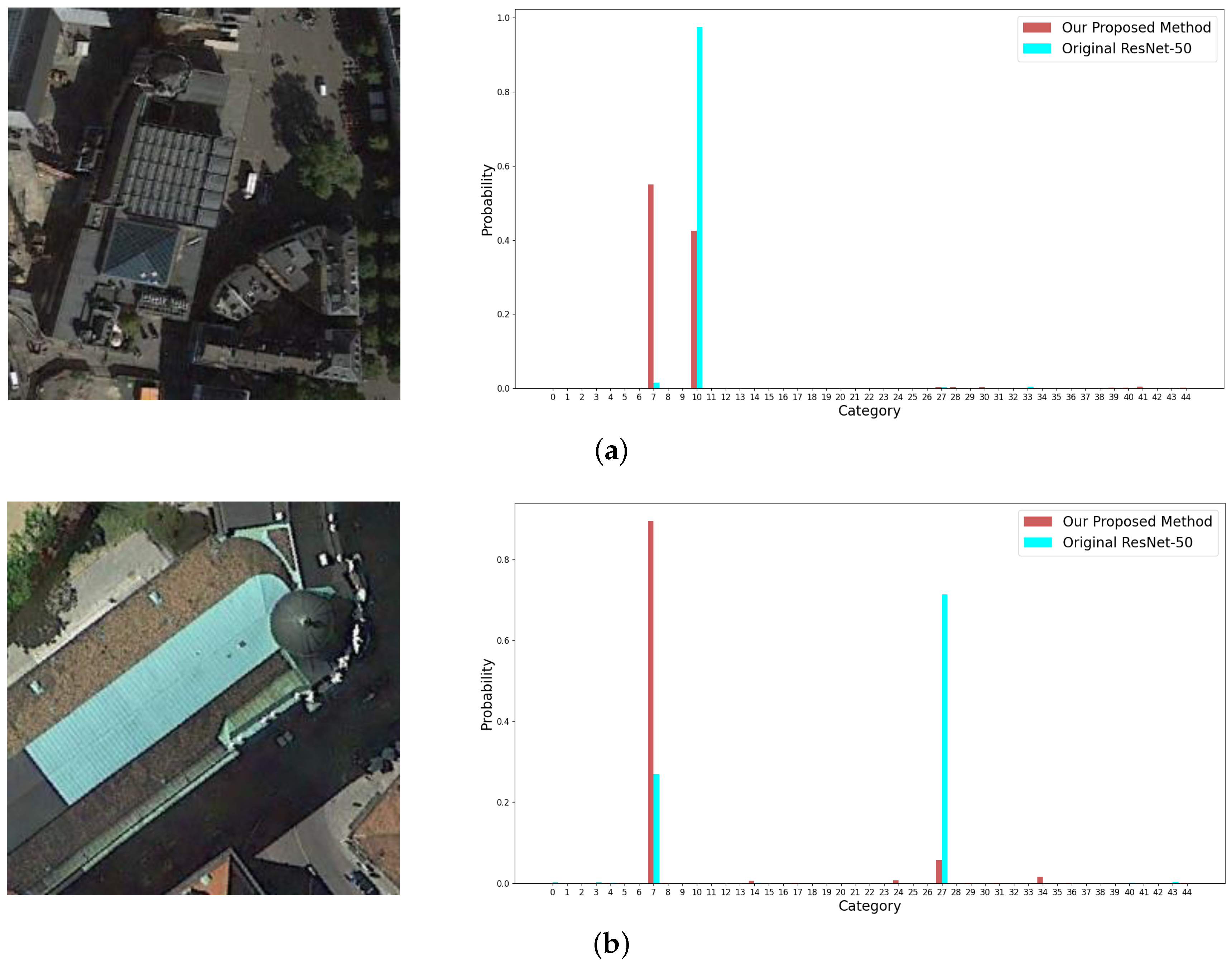
The issues of high inter-class similarity and high intra-class variance are challenging to remote sensing scene image classification. In Figure 14, two images labelled as medium residential and dense residential are tested to show the proposed strategy can reduce the inter-class similarity. In Figure 15, the reduction of intra-class variance is validated.
The images from top to bottom in Figure 14 are misclassified as #11 (dense residential) and #23 (medium residential) by ResNet-50 which is difficult to discriminate the samples between the two categories because of high inter-class similarity. By contrast, our method produces a very high score for the correct category in Figure 14b, which demonstrates the ability to learn a more proper decision boundary between the two categories than ResNet-50. Regarding the image in Figure 14a which exhibits a challenging case, our method can still present a correct prediction.
The images from top to bottom in Figure 15 are misclassified as #10 (commercial area) and #27 (palace) by ResNet-50 due to high intra-class variance of the church category. Instead, in Figure 15b, our method learns the universal features of the church category and thus, produces a very high score on the correct category. In Figure 15a, our method obtains a correct result on the challenging sample, where the top two scores are very close to each other.
6. Conclusions
In this paper, we propose an adaptive decision-level fusion framework to improve the performance of the existing deep CNN models in remote sensing image scene classification. The architecture consists of a backbone network, a pluginable importance factor generator, multiple classifiers, and a decision fusion module. Each sub-classifier predicts the classification scores based on the features of different stages. The importance factor generator is used to adaptively assign an importance factor to each classification score in each stage. The factors and the scores are then fused to produce the final classification result. This framework not only achieves information fusion across different scales but also reduces the inter-class similarity and the intra-class variance which are obstacles in remote sensing scene classification. In addition, we further propose the stochastic decision-level fusion training strategy, which selectively enables the classification scores of each stage to participate in the decision-level fusion process during training. Experiments on four popular remote sensing image datasets validate the superiority of our adaptive decision-level fusion architecture and the stochastic decision-level fusion training strategy.
Author Contributions
Conceptualization, J.S. and R.W.; methodology, J.S., C.Z. and R.W.; software, C.Z.; validation, C.Z.; formal analysis, J.S., R.W. and Y.Z.; investigation, J.S. and Y.Z.; resources, R.W. and Y.Z.; data curation, Y.Z.; writing—original draft preparation, J.S.; writing—review and editing, R.W.; visualization, C.Z.; supervision, J.S., R.W. and Y.Z.; project administration, J.S. and R.W.; funding acquisition, J.S. All authors have read and agreed to the published version of the manuscript.
Funding
This research was funded by National Natural Science Foundation of China grant numbers 61603233 and 51909206, and the Project for “1000 Talents Plan for Young Talents of Yunnan Province”.
Institutional Review Board Statement
Not applicable.
Informed Consent Statement
Not applicable.
Data Availability Statement
The data used to support the findings of this study are available from the corresponding author upon request.
Acknowledgments
The authors wish to acknowledge the Key Laboratory of Underwater Intelligent Equipment of Henan Province for offering strong support throughout the experiments.
Conflicts of Interest
The authors declare no conflict of interest.
References
- Cheng, G.; Han, J.; Lu, X. Remote sensing image scene classification: Benchmark and state of the art. Proc. IEEE 2017, 105, 1865–1883. [Google Scholar] [CrossRef] [Green Version]
- Martha, T.R.; Kerle, N.; van Westen, C.J.; Jetten, V.; Kumar, K.V. Segment optimization and data-driven thresholding for knowledge-based landslide detection by object-based image analysis. IEEE Trans. Geosci. Remote Sens. 2011, 49, 4928–4943. [Google Scholar] [CrossRef]
- Kim, M.; Madden, M.; Warner, T.A. Forest type mapping using object-specific texture measures from multispectral Ikonos imagery. Photogramm. Eng. Remote Sens. 2009, 75, 819–829. [Google Scholar] [CrossRef] [Green Version]
- Cheng, G.; Han, J.; Zhou, P.; Guo, L. Multi-class geospatial object detection and geographic image classification based on collection of part detectors. ISPRS J. Photogramm. Remote Sens. 2014, 98, 119–132. [Google Scholar] [CrossRef]
- Zhu, Q.; Zhong, Y.; Zhao, B.; Xia, G.S.; Zhang, L. Bag-of-visual-words scene classifier with local and global features for high spatial resolution remote sensing imagery. IEEE Geosci. Remote Sens. Lett. 2016, 13, 747–751. [Google Scholar] [CrossRef]
- Chaib, S.; Gu, Y.; Yao, H. An informative feature selection method based on sparse PCA for VHR scene classification. IEEE Geosci. Remote Sens. Lett. 2015, 13, 147–151. [Google Scholar] [CrossRef]
- Ke, Y.; Sukthankar, R. PCA-SIFT: A more distinctive representation for local image descriptors. In Proceedings of the 2004 IEEE Computer Society Conference on Computer Vision and Pattern Recognition (CVPR), Washington, DC, USA, 27 June–2 July 2004; Volume 2, pp. 506–513. [Google Scholar]
- Dalal, N.; Triggs, B. Histograms of oriented gradients for human detection. In Proceedings of the 2005 IEEE Computer Society Conference on Computer Vision and Pattern Recognition (CVPR), San Diego, CA, USA, 20–25 June 2005; Volume 1, pp. 886–893. [Google Scholar]
- Zhao, F.; Sun, H.; Liu, S.; Zhou, S. Combining low level features and visual attributes for VHR remote sensing image classification. In Proceedings of the MIPPR 2015: Remote Sensing Image Processing, Geographic Information Systems, and Other Applications, International Society for Optics and Photonics, Enshi, China, 14 December 2015; Volume 9815, p. 98150C. [Google Scholar]
- Yu, X.; Wu, X.; Luo, C.; Ren, P. Deep learning in remote sensing scene classification: A data augmentation enhanced convolutional neural network framework. GISci. Remote Sens. 2017, 54, 741–758. [Google Scholar] [CrossRef] [Green Version]
- Zhou, W.; Shao, Z.; Cheng, Q. Deep feature representations for high-resolution remote sensing scene classification. In Proceedings of the 2016 IEEE International Workshop on Earth Observation and Remote Sensing Applications (EORSA), Guangzhou, China, 4–6 June 2016; pp. 338–342. [Google Scholar]
- Cheng, G.; Ma, C.; Zhou, P.; Yao, X.; Han, J. Scene classification of high resolution remote sensing images using convolutional neural networks. In Proceedings of the 2016 IEEE International Geoscience and Remote Sensing Symposium (IGARSS), Beijing, China, 10–15 July 2016; pp. 767–770. [Google Scholar]
- Lan, M.; Zhang, Y.; Zhang, L.; Du, B. Global context based automatic road segmentation via dilated convolutional neural network. Inf. Sci. 2020, 535, 156–171. [Google Scholar] [CrossRef]
- Liu, J.; Zhong, Q.; Yuan, Y.; Su, H.; Du, B. SemiText: Scene text detection with semi-supervised learning. Neurocomputing 2020, 407, 343–353. [Google Scholar] [CrossRef]
- Hu, M.; Wu, C.; Zhang, L.; Du, B. Hyperspectral Anomaly Change Detection Based on Autoencoder. IEEE J. Sel. Top. Appl. Earth Obs. Remote Sens. 2021, 14, 3750–3762. [Google Scholar] [CrossRef]
- Dong, Y.; Zhang, Q. A Combined Deep Learning Model for the Scene Classification of High-Resolution Remote Sensing Image. IEEE Geosci. Remote Sens. Lett. 2019, 16, 1540–1544. [Google Scholar] [CrossRef]
- Xu, K.; Huang, H.; Deng, P.; Shi, G. Two-stream feature aggregation deep neural network for scene classification of remote sensing images. Inf. Sci. 2020, 539, 250–268. [Google Scholar] [CrossRef]
- Fang, J.; Yuan, Y.; Lu, X.; Feng, Y. Robust space–frequency joint representation for remote sensing image scene classification. IEEE Trans. Geosci. Remote Sens. 2019, 57, 7492–7502. [Google Scholar] [CrossRef]
- Shi, C.; Wang, T.; Wang, L. Branch Feature Fusion Convolution Network for Remote Sensing Scene Classification. IEEE J. Sel. Top. Appl. Earth Obs. Remote Sens. 2020, 13, 5194–5210. [Google Scholar] [CrossRef]
- Xu, K.; Huang, H.; Li, Y.; Shi, G. Multilayer feature fusion network for scene classification in remote sensing. IEEE Geosci. Remote Sens. Lett. 2020, 17, 1894–1898. [Google Scholar] [CrossRef]
- Cheng, G.; Yang, C.; Yao, X.; Guo, L.; Han, J. When deep learning meets metric learning: Remote sensing image scene classification via learning discriminative CNNs. IEEE Trans. Geosci. Remote Sens. 2018, 56, 2811–2821. [Google Scholar] [CrossRef]
- Wei, T.; Wang, J.; Liu, W.; Chen, H.; Shi, H. Marginal center loss for deep remote sensing image scene classification. IEEE Geosci. Remote Sens. Lett. 2019, 17, 968–972. [Google Scholar] [CrossRef]
- Hinton, G.E.; Srivastava, N.; Krizhevsky, A.; Sutskever, I.; Salakhutdinov, R.R. Improving neural networks by preventing co-adaptation of feature detectors. arXiv 2012, arXiv:1207.0580. [Google Scholar]
- Nogueira, K.; Penatti, O.A.; Dos Santos, J.A. Towards better exploiting convolutional neural networks for remote sensing scene classification. Pattern Recognit. 2017, 61, 539–556. [Google Scholar] [CrossRef] [Green Version]
- Zhang, F.; Du, B.; Zhang, L. Scene classification via a gradient boosting random convolutional network framework. IEEE Trans. Geosci. Remote Sens. 2016, 54, 1793–1802. [Google Scholar] [CrossRef]
- Shen, J.; Zhang, T.; Wang, Y.; Wang, R.; Wang, Q.; Qi, M. A Dual-Model Architecture with Grouping-Attention-Fusion for Remote Sensing Scene Classification. Remote Sens. 2021, 13, 433. [Google Scholar] [CrossRef]
- Zhang, W.; Tang, P.; Zhao, L. Remote sensing image scene classification using CNN-CapsNet. Remote Sens. 2019, 11, 494. [Google Scholar] [CrossRef] [Green Version]
- Dede, M.A.; Aptoula, E.; Genc, Y. Deep network ensembles for aerial scene classification. IEEE Geosci. Remote Sens. Lett. 2018, 16, 732–735. [Google Scholar] [CrossRef]
- Shi, C.; Zhao, X.; Wang, L. A Multi-Branch Feature Fusion Strategy Based on an Attention Mechanism for Remote Sensing Image Scene Classification. Remote Sens. 2021, 13, 1950. [Google Scholar] [CrossRef]
- Lu, X.; Sun, H.; Zheng, X. A feature aggregation convolutional neural network for remote sensing scene classification. IEEE Trans. Geosci. Remote Sens. 2019, 57, 7894–7906. [Google Scholar] [CrossRef]
- Sun, H.; Li, S.; Zheng, X.; Lu, X. Remote sensing scene classification by gated bidirectional network. IEEE Trans. Geosci. Remote Sens. 2019, 58, 82–96. [Google Scholar] [CrossRef]
- Ji, J.; Zhang, T.; Jiang, L.; Zhong, W.; Xiong, H. Combining multilevel features for remote sensing image scene classification with attention model. IEEE Geosci. Remote Sens. Lett. 2019, 17, 1647–1651. [Google Scholar] [CrossRef]
- Yu, D.; Guo, H.; Xu, Q.; Lu, J.; Zhao, C.; Lin, Y. Hierarchical Attention and Bilinear Fusion for Remote Sensing Image Scene Classification. IEEE J. Sel. Top. Appl. Earth Obs. Remote Sens. 2020, 13, 6372–6383. [Google Scholar] [CrossRef]
- Zhang, D.; Li, N.; Ye, Q. Positional context aggregation network for remote sensing scene classification. IEEE Geosci. Remote Sens. Lett. 2019, 17, 943–947. [Google Scholar] [CrossRef]
- Li, X.; Jiang, B.; Sun, T.; Wang, S. Remote sensing scene classification based on decision-level fusion. In Proceedings of the 2018 IEEE Information Technology and Mechatronics Engineering Conference (ITOEC), Chongqing, China, 14–16 December 2018; pp. 393–397. [Google Scholar]
- Wang, Q.; Huang, W.; Xiong, Z.; Li, X. Looking Closer at the Scene: Multiscale Representation Learning for Remote Sensing Image Scene Classification. IEEE Trans. Neural Netw. Learn. Syst. 2020, 1, 1–15. [Google Scholar]
- Yang, Y.; Newsam, S. Bag-of-visual-words and spatial extensions for land-use classification. In Proceedings of the 18th SIGSPATIAL International Conference on Advances in Geographic Information Systems (ACM SIGSPATIAL), San Jose, CA, USA, 2–5 November 2010; pp. 270–279. [Google Scholar]
- Zou, Q.; Ni, L.; Zhang, T.; Wang, Q. Deep learning based feature selection for remote sensing scene classification. IEEE Geosci. Remote Sens. Lett. 2015, 12, 2321–2325. [Google Scholar] [CrossRef]
- Xia, G.S.; Hu, J.; Hu, F.; Shi, B.; Bai, X.; Zhong, Y.; Zhang, L.; Lu, X. AID: A benchmark data set for performance evaluation of aerial scene classification. IEEE Trans. Geosci. Remote Sens. 2017, 55, 3965–3981. [Google Scholar] [CrossRef] [Green Version]
- He, K.; Zhang, X.; Ren, S.; Sun, J. Deep residual learning for image recognition. In Proceedings of the IEEE Conference on Computer Vision and Pattern Recognition (CVPR), Las Vegas, NV, USA, 27–30 June 2016; pp. 770–778. [Google Scholar]
- Zhang, B.; Zhang, Y.; Wang, S. A lightweight and discriminative model for remote sensing scene classification with multidilation pooling module. IEEE J. Sel. Top. Appl. Earth Obs. Remote Sens. 2019, 12, 2636–2653. [Google Scholar] [CrossRef]
- Song, S.; Yu, H.; Miao, Z.; Zhang, Q.; Lin, Y.; Wang, S. Domain adaptation for convolutional neural networks-based remote sensing scene classification. IEEE Geosci. Remote Sens. Lett. 2019, 16, 1324–1328. [Google Scholar] [CrossRef]
- Li, B.; Su, W.; Wu, H.; Li, R.; Zhang, W.; Qin, W.; Zhang, S. Aggregated deep fisher feature for VHR remote sensing scene classification. IEEE J. Sel. Top. Appl. Earth Obs. Remote Sens. 2019, 12, 3508–3523. [Google Scholar] [CrossRef]
- Lv, Y.; Zhang, X.; Xiong, W.; Cui, Y.; Cai, M. An end-to-end local-global-fusion feature extraction network for remote sensing image scene classification. Remote Sens. 2019, 11, 3006. [Google Scholar] [CrossRef] [Green Version]
- Anwer, R.M.; Khan, F.S.; van de Weijer, J.; Molinier, M.; Laaksonen, J. Binary patterns encoded convolutional neural networks for texture recognition and remote sensing scene classification. ISPRS J. Photogramm. Remote Sens. 2018, 138, 74–85. [Google Scholar] [CrossRef] [Green Version]
- Liu, X.; Zhou, Y.; Zhao, J.; Yao, R.; Liu, B.; Zheng, Y. Siamese convolutional neural networks for remote sensing scene classification. IEEE Geosci. Remote Sens. Lett. 2019, 16, 1200–1204. [Google Scholar] [CrossRef]
- Liu, B.D.; Meng, J.; Xie, W.Y.; Shao, S.; Li, Y.; Wang, Y. Weighted spatial pyramid matching collaborative representation for remote-sensing-image scene classification. Remote Sens. 2019, 11, 518. [Google Scholar] [CrossRef] [Green Version]
- Zhou, Y.; Liu, X.; Zhao, J.; Ma, D.; Yao, R.; Liu, B.; Zheng, Y. Remote sensing scene classification based on rotation-invariant feature learning and joint decision making. EURASIP J. Image Video Process. 2019, 2019, 1–11. [Google Scholar] [CrossRef] [Green Version]
- Qi, K.; Yang, C.; Hu, C.; Shen, Y.; Shen, S.; Wu, H. Rotation Invariance Regularization for Remote Sensing Image Scene Classification with Convolutional Neural Networks. Remote Sens. 2021, 13, 569. [Google Scholar] [CrossRef]
- He, N.; Fang, L.; Li, S.; Plaza, A.; Plaza, J. Remote sensing scene classification using multilayer stacked covariance pooling. IEEE Trans. Geosci. Remote Sens. 2018, 56, 6899–6910. [Google Scholar] [CrossRef]
- Wang, Q.; Liu, S.; Chanussot, J.; Li, X. Scene classification with recurrent attention of VHR remote sensing images. IEEE Trans. Geosci. Remote Sens. 2018, 57, 1155–1167. [Google Scholar] [CrossRef]
- Zeng, D.; Chen, S.; Chen, B.; Li, S. Improving remote sensing scene classification by integrating global-context and local-object features. Remote Sens. 2018, 10, 734. [Google Scholar] [CrossRef] [Green Version]
- Li, Z.; Xu, K.; Xie, J.; Bi, Q.; Qin, K. Deep multiple instance convolutional neural networks for learning robust scene representations. IEEE Trans. Geosci. Remote Sens. 2020, 58, 3685–3702. [Google Scholar] [CrossRef]
Figure 1.
Examples from the NWPU-RESISC 45 dataset. The small objects in the images are critical to the classification of the scene.
Figure 1.
Examples from the NWPU-RESISC 45 dataset. The small objects in the images are critical to the classification of the scene.

Figure 2.
Illustration of the high inter-class similarity and high intra-class variance in the remote sensing image dataset. (a) Illustrates four images with different appearances, which are labelled as church. (b) Shows dense residential in the left two images, and medium residential in the right two images.

Figure 3.
The framework of the proposed adaptive decision-level fusion method. From top to bottom, the blue blocks represent different stages of a deep CNN backbone; the light blue rectangles with round corners are the classifiers based on the features of different stages; the green block is the importance factor generator, which is used to generate the importance factor matrix composed from “” to “”; the grey blocks named as “Lock 1” to “Lock 4” represent the stochastic decision-level fusion process.

Figure 4.
The importance factor generator.

Figure 5.
An exemplar demonstration of the intra-class variance and inter-class similarity. The figures plot the output scores by ResNet-50 in (a,b) and that by our method in (c,d) for all images in the NWPU-RESISC 45 dataset. In (a,c), the blue points represent the predicted church probability of each image belonging on the true church class. In (b,d), the blue and yellow points represent the predicted probabilities on dense residential and medium residential, respectively, where the images actually belong to the dense residential class.

Figure 6.
The stochastic decision-level fusion training strategy. The detailed backbones and classifiers are omitted. The blue and purple rectangles represent different stages. The green circles with “1” indicate the classification scores that participate in the fusion process, while the red circles with “0” do not participate.

Figure 7.
The performance of the proposed method with different survival rates.

Figure 8.
The confusion matrix on the UCM dataset under the 50% training samples.

Figure 9.
The confusion matrix on the RSSCN 7 dataset under the 50% training samples.

Figure 10.
The confusion matrix on the AID dataset under the 50% training samples.

Figure 11.
The confusion matrix for the NWPU-RESISC 45 dataset under the 20% training samples.

Figure 12.
Visualization of the output scores in different stages. (a–d) illustrate the results of the images belonging to buildings, storage tanks, intersection, and dense residential respectively. All the selected images are correctly classified by the adaptive fusion method, as indicated by the purple lines.

Figure 13.
Examples from the NWPU-RESISC 45 dataset with small objects and the corresponding output probabilities of categories by the original ResNet-50 (plotted in blue columns) and by our proposed method (plotted in red columns). The images in (a–c) are labelled as airplane, basketball court, and island, respectively.


Figure 14.
Examples from the NWPU-RESISC 45 dataset and the corresponding output probabilities of categories by the original ResNet-50 (plotted in blue columns) and by our proposed method (plotted in red columns). The images in (a,b) are labelled as medium residential and dense residential, respectively.


Figure 15.
Examples from the NWPU-RESISC 45 dataset and the corresponding output probabilities of categories by the original ResNet-50 (plotted in blue columns) and by our proposed method (plotted in red columns). The images in (a,b) are both labelled as church.
Figure 15.
Examples from the NWPU-RESISC 45 dataset and the corresponding output probabilities of categories by the original ResNet-50 (plotted in blue columns) and by our proposed method (plotted in red columns). The images in (a,b) are both labelled as church.


Table 1.
Comparison of sizes of the models before and after improvement.
| Model | Parameters (MB) | |||
|---|---|---|---|---|
| UCM | RSSCN 7 | AID | NWPU 45 | |
| ResNet-50 | 23.55 | 23.52 | 23.57 | 23.60 |
| Ours | 24.11 | 24.25 | 24.01 | 23.85 |
| Increment (%) | 2.4 | 3.1 | 1.9 | 1.1 |
Table 2.
Comparison of the FLOPs of the models before and after improvement.
| Model | FLOPs (MB) | |||
|---|---|---|---|---|
| UCM | RSSCN 7 | AID | NWPU 45 | |
| ResNet-50 | 4087.18 | 4087.15 | 4087.20 | 4087.23 |
| Ours | 4098.06 | 4092.18 | 4098.86 | 4095.05 |
| Increment (%) | 0.3 | 0.1 | 0.3 | 0.2 |
Table 3.
The performance comparison on RSSCN 7 dataset with different backbones. SDFTS represents the stochastic decision-level fusion training strategy. The bold values denote the best performance on different backbones.
Table 3.
The performance comparison on RSSCN 7 dataset with different backbones. SDFTS represents the stochastic decision-level fusion training strategy. The bold values denote the best performance on different backbones.
| Method | 50% for Training |
|---|---|
| Fine_tune MobileNet V2 [41] | 92.46 ± 0.66 |
| Ours (MobileNet V2) | 94.21 ± 0.56 |
| Ours+SDFTS (MobileNet V2) | 94.59 ± 0.32 |
| Fine_tune VGG-16 [42] | 93.00 |
| Ours (VGG-16) | 94.72 ± 0.42 |
| Ours+SDFTS (VGG-16) | 95.70 ± 0.28 |
| Fine_tune ResNet-50 [42] | 92.29 |
| Ours (ResNet-50) | 95.15 ± 0.64 |
| Ours+SDFTS (ResNet-50) | 95.49 ± 0.55 |
| Fine_tune ResNet-152 [42] | 91.36 |
| Ours (ResNet-152) | 95.09 ± 0.47 |
| Ours+SDFTS (ResNet-152) | 95.76 ± 0.34 |
Table 4.
The setting of survival rate in different classification tasks.
| Dataset | UCM | RSSCN7 | AID | NWPU 45 | |||
|---|---|---|---|---|---|---|---|
| Training ratio | 50% | 80% | 50% | 20% | 50% | 10% | 20% |
| Survival rate | 0.9 | 0.8 | 0.8 | 0.8 | 0.9 | 0.8 | 0.6 |
Table 5.
The performance comparison on the UC Merced Land-Use dataset. SDFTS represents the stochastic decision-level fusion training strategy. The bold values denote the best performance of different training ratio.
Table 5.
The performance comparison on the UC Merced Land-Use dataset. SDFTS represents the stochastic decision-level fusion training strategy. The bold values denote the best performance of different training ratio.
| Method | 50% for Training | 80% for Training |
|---|---|---|
| ResNet-50 | 97.22 ± 0.45 | 98.81 ± 0.51 |
| ADFF [43] | 97.22 ± 0.45 | 98.81 ± 0.51 |
| Standard RGB [45] | 96.22 ± 0.38 | 96.80 ± 0.51 |
| TEX-Net-LF [45] | 96.91 ± 0.36 | 97.72 ± 0.54 |
| SiameseNet [46] | 90.95 | 94.29 |
| PANet50 [34] | - | 99.21 ± 0.18 |
| HABFNet [33] | 98.47 ± 0.47 | 99.29 ± 0.35 |
| SPM-CRC [47] | - | 97.95 |
| WSPM-CRC [47] | - | 97.95 |
| R.D [48] | 91.71 | 94.76 |
| RIR+ResNet50 [49] | 98.28 ± 0.34 | 99.15 ± 0.40 |
| GBNet [31] | 97.05 ± 0.19 | 98.57 ± 0.48 |
| MSCP+MRA [50] | - | 98.40 ± 0.34 |
| FACNN [30] | - | 98.81 ± 0.24 |
| ResNet_LGFFE [44] | - | 98.62 ± 0.88 |
| ARCNet [51] | 96.81 ± 0.14 | 99.12 ± 0.40 |
| DCNN [21] | - | 98.93 ± 0.10 |
| Proposed [52] | 97.37 ± 0.44 | 99 ± 0.35 |
| Ours | 98.65 ± 0.49 | 99.71 ± 0.21 |
| Ours+SDFTS | 98.90 ± 0.47 | 99.64 ± 0.16 |
Table 6.
The performance comparison on the RSSCN 7 dataset. SDFTS represents the stochastic decision-level fusion training strategy. The bold values denote the best performance of different training ratio.
Table 6.
The performance comparison on the RSSCN 7 dataset. SDFTS represents the stochastic decision-level fusion training strategy. The bold values denote the best performance of different training ratio.
| Method | 50% for Training |
|---|---|
| VGG 16 | 93.00 |
| ResNet-50 | 92.29 |
| Standard RGB [45] | 93.12 ± 0.55 |
| TEX-Net-LF [45] | 94.00 ± 0.57 |
| SPM-CRC [47] | 93.86 |
| WSPM-CRC [47] | 93.9 |
| Proposed [42] | 93.14 |
| ADFF [43] | 95.21 ± 0.50 |
| LCNN-BFF [19] | 94.64 ± 0.21 |
| Ours | 95.15 ± 0.64 |
| Ours+SDFTS | 95.49 ± 0.55 |
Table 7.
The performance comparison for the AID dataset. SDFTS represents the stochastic decision-level fusion training strategy. The bold values denote the best performance of different training ratio.
Table 7.
The performance comparison for the AID dataset. SDFTS represents the stochastic decision-level fusion training strategy. The bold values denote the best performance of different training ratio.
| Method | 20% for Training | 50% for Training |
|---|---|---|
| ResNet50 | 86.48 ± 0.49 | 89.22 ± 0.34 |
| Standard RGB [45] | 88.79 ± 0.19 | 92.33 ± 0.13 |
| TEX-Net-LF [45] | 93.81 ± 0.12 | 95.73 ± 0.16 |
| SPM-CRC [47] | - | 95.1 |
| WSPM-CRC [47] | - | 95.11 |
| GBNet [31] | 92.20 ± 0.23 | 95.48 ± 0.12 |
| MSCP+MRA [50] | 92.21 ± 0.17 | 96.56 ± 0.18 |
| FACNN [30] | - | 95.45 ± 0.11 |
| MF2Net [20] | 93.82 ± 0.26 | 95.93 ± 0.23 |
| TFADNN [17] | 93.21 ± 0.32 | 95.64 ± 0.16 |
| ARCNet [51] | 88.75 ± 0.40 | 93.10 ± 0.55 |
| DCNN [21] | 90.82 ± 0.16 | 96.89 ± 0.10 |
| ResNet_LGFFE [44] | 90.83 ± 0.55 | 94.46 ± 0.48 |
| Ours | 94.69 ± 0.23 | 96.67 ± 0.28 |
| Ours+SDFTS | 95.05 ± 0.24 | 97.04 ± 0.20 |
Table 8.
The performance comparison for the NWPU-RESISC 45 dataset. SDFTS represents the stochastic decision-level fusion training strategy. The bold values denote the best performance of different training ratio.
Table 8.
The performance comparison for the NWPU-RESISC 45 dataset. SDFTS represents the stochastic decision-level fusion training strategy. The bold values denote the best performance of different training ratio.
| Method | 10% for Training | 20% for Training |
|---|---|---|
| ResNet-50 | 89.88 ± 0.26 | 92.35 ± 0.19 |
| ADFF [43] | 86.01 ± 0.15 | 88.79 ± 0.17 |
| RIR [49] | 92.05 ± 0.23 | 94.06 ± 0.15 |
| SiameseNet [46] | - | 92.28 |
| R.D [48] | - | 92.67 |
| MI-VGG-16 [53] | 91.47 ± 0.20 | 93.14 ± 0.16 |
| MSCP+MRA [50] | 88.07 ± 0.18 | 90.81 ± 0.13 |
| MF2Net [20] | 90.17 ± 0.25 | 92.73 ± 0.21 |
| TFADNN [17] | 87.78 ± 0.11 | 90.86 ± 0.24 |
| LCNN-BFF [19] | 86.53 ± 0.15 | 91.73 ± 0.17 |
| DCNN [21] | 89.22 ± 0.50 | 91.89 ± 0.22 |
| Ours | 91.47 ± 0.41 | 94.11 ± 0.16 |
| Ours+SDFTS | 92.03 ± 0.23 | 94.40 ± 0.13 |
Publisher’s Note: MDPI stays neutral with regard to jurisdictional claims in published maps and institutional affiliations. |
© 2021 by the authors. Licensee MDPI, Basel, Switzerland. This article is an open access article distributed under the terms and conditions of the Creative Commons Attribution (CC BY) license (https://creativecommons.org/licenses/by/4.0/).
Share and Cite
MDPI and ACS Style
Shen, J.; Zhang, C.; Zheng, Y.; Wang, R. Decision-Level Fusion with a Pluginable Importance Factor Generator for Remote Sensing Image Scene Classification. Remote Sens. 2021, 13, 3579. https://0-doi-org.brum.beds.ac.uk/10.3390/rs13183579
AMA Style
Shen J, Zhang C, Zheng Y, Wang R. Decision-Level Fusion with a Pluginable Importance Factor Generator for Remote Sensing Image Scene Classification. Remote Sensing. 2021; 13(18):3579. https://0-doi-org.brum.beds.ac.uk/10.3390/rs13183579
Chicago/Turabian StyleShen, Junge, Chi Zhang, Yu Zheng, and Ruxin Wang. 2021. "Decision-Level Fusion with a Pluginable Importance Factor Generator for Remote Sensing Image Scene Classification" Remote Sensing 13, no. 18: 3579. https://0-doi-org.brum.beds.ac.uk/10.3390/rs13183579
Note that from the first issue of 2016, this journal uses article numbers instead of page numbers. See further details here.