Article

The Potential of Satellite Remote Sensing Time Series to Uncover Wetland Phenology under Unique Challenges of Tidal Setting

by
Gwen Joelle Miller
1,*,
Iryna Dronova
1,2,
Patricia Y. Oikawa
3,
Sara Helen Knox
4,
Lisamarie Windham-Myers
5,
Julie Shahan
3 and
Ellen Stuart-Haëntjens
6
1
Landscape Architecture and Environmental Planning, University of California at Berkeley, Berkeley, CA 94720, USA
2
Department of Environmental Sciences, Policy and Management, Rausser College of Natural Resources, University of California, Berkeley, CA 94720, USA
3
Department of Earth and Environmental Sciences, California State University, East Bay, Hayward, CA 94542, USA
4
Department of Geography, The University of British Columbia, Vancouver, BC V6T 1Z2, Canada
5
U.S. Geological Survey, Water Mission Area, Menlo Park, CA 94025, USA
6
U.S. Geological Survey, California Water Science Center Sacramento, Sacramento, CA 95819, USA
*
Author to whom correspondence should be addressed.
Remote Sens. 2021, 13(18), 3589; https://0-doi-org.brum.beds.ac.uk/10.3390/rs13183589
Submission received: 30 July 2021 / Revised: 28 August 2021 / Accepted: 1 September 2021 / Published: 9 September 2021
(This article belongs to the Special Issue Remote Sensing of Coastal Processes)

Abstract

:
While growth history of vegetation within upland systems is well studied, plant phenology within coastal tidal systems is less understood. Landscape-scale, satellite-derived indicators of plant greenness may not adequately represent seasonality of vegetation biomass and productivity within tidal wetlands due to limitations of cloud cover, satellite temporal frequency, and attenuation of plant signals by tidal flooding. However, understanding plant phenology is necessary to gain insight into aboveground biomass, photosynthetic activity, and carbon sequestration. In this study, we use a modeling approach to estimate plant greenness throughout a year in tidal wetlands located within the San Francisco Bay Area, USA. We used variables such as EVI history, temperature, and elevation to predict plant greenness on a 14-day timestep. We found this approach accurately estimated plant greenness, with larger error observed within more dynamic restored wetlands, particularly at early post-restoration stages. We also found modeled EVI can be used as an input variable into greenhouse gas models, allowing for an estimate of carbon sequestration and gross primary production. Our strategy can be further developed in future research by assessing restoration and management effects on wetland phenological dynamics and through incorporating the entire Sentinel-2 time series once it becomes available within Google Earth Engine.

Graphical Abstract

1. Introduction

Remote sensing products are increasingly important to facilitate upscaling of critical ecosystem services such as carbon (C) sequestration from local monitoring sites to regional extents of management and planning [1,2,3]. Such efforts often utilize spatially explicit time series of spectral vegetation indices (or “greenness”) that can provide useful proxies of plant biomass, coverage, and photosynthetic activity (e.g., [4,5,6]). Predicting such vegetation properties at different stages of a growing season enables a better understanding of various biotic and abiotic controls on plant and ecosystem functioning [7,8,9] and modeling of ecosystem services targeted by management, restoration, and conservation efforts. However, in contrast to well-studied “upland” ecosystems, this potential remains less certain in coastal environments such as tidal marshes, where high short-term spectral variability precludes accurate characterization of vegetation (e.g., [10,11,12,13,14]). This uncertainty contributes to gaps in upscaling and budgeting of these important “blue carbon” ecosystems and projecting their future under climatic, hydrological, and anthropogenic change drivers [15,16,17].
From a remote sensing perspective, the key driver behind this issue is variable tidal flooding, which leads to attenuation of vegetation signals [14,18] and limits the ability of spectral reflectance from snapshot remote observations to indicate relevant aspects of plant physiology and abundance. Furthermore, such attenuation non-linearly increases with the magnitude of flooding [14], limiting performance of vegetation indicators more substantially in frequently flooded environments such as low-elevation zones of tidal marshes. Yet, correcting for flooding is not a straightforward task because the net effect of attenuation depends not only on tidal stage and local ground elevation, but also on vegetation canopy properties (height, biomass, structure) that define to what extent vegetation can be obscured by flooding at a given point in a season [4,19]. The interplay among these factors affects how much vegetation is effectively “visible” to a remote sensor at the time of overpass in a given part of a wetland.
Characterizing this interplay in a tidal setting is extremely difficult due to the lack of relevant geospatial and earth observation data at sufficiently high temporal frequencies. Among various instruments and platforms, light detection and ranging (LiDAR) systems are currently best suited for characterizing both ground elevation and vegetation height and for modeling local inundation based on these characteristics [20,21,22]. However, in the absence of continuous global LiDAR observations at high spatial resolutions, acquisitions of such data at local and regional scales remain patchy, sporadic, and too costly for matching temporal frequencies of tidal variation (e.g., from hourly to biweekly). Furthermore, in tidal wetlands the accuracy of LiDAR-derived metrics may be compromised by variation in the soil/sediment and by the obstruction of soil by dense vegetation and dead biomass, or litter [21,23]. These issues limit the potential for tracking spatial and temporal (seasonal) dynamics of wetland vegetation biomass and height which modulate tidal attenuation during the growing season. This limitation is amplified by the common lack of alternative up-to-date wetland vegetation products, e.g., plant community- or species-level maps at sufficiently high spatial resolution and temporal frequency to help approximate changes in biomass and canopy properties at a local scale [24].
Previous studies have offered several strategies to help circumvent these challenges to summarize spatio-temporal variability of wetland vegetation for tidal ecosystem mapping, modeling, and phenological assessments. For example, the first USA national-scale model of aboveground tidal marsh C stocks [24] focused on the relationships between field-measured biomass and temporally matching satellite products across a comprehensive range of sites and vegetation types, often sampled at or close to the peak biomass stage. Peak biomass conditions reduce the magnitude of tidal attenuation and provide a way to characterize the overall biomass and C stock representative of a given ecosystem, which can be useful for annual C budgeting [25,26]. In other cases, it may be necessary to explicitly consider seasonal variation in vegetation proxies to indicate shorter-term changes in biogeochemical fluxes and wetland habitat for specific seasonal phases of animal ecological cycles [5,6,7], which in tidal settings requires addressing flooding-induced attenuation specific to the time and location of satellite observations [16]. A study of tidal marsh vegetation phenology in three Pacific Coast sites [27] incorporated the offsets in water level height between the tidal gauge data from individual site locations into models of vegetation phenology, and additionally removed satellite images collected at high water levels. Alternatively, high temporal frequency remote sensing data can be used to identify and flag conditions when a given pixel is likely to be flooded relative to its overall phenological behavior, such as the Tidal Marsh Inundation Index [16] based on 500 m MODIS satellite reflectance products in green and shortwave infrared electromagnetic regions.
Such methods, however, may be less feasible when satellite time series with optimal spatial resolution are sparser and compromised by clouds, which increases the uncertainty associated with exclusion of high-tide images, especially in sites with no accurate local tidal data. Furthermore, from an ecosystem modeling perspective, high-tide dates are still informative of how tidal flooding affects ecosystem functioning; for instance, the rate of carbon uptake by flooded vegetation during photosynthetically active daytime hours may be expected to differ between flooded and non-flooded conditions [3,28]. As the contribution of tidal vegetation biomass to remote sensing signals is expected to increase with the increment in biomass and height over the course of the growing season [28], the degree of attenuation reduces during the peak biomass stages. Thus, rather than predicting the total amount of vegetation, studies aiming to support biogeochemical and habitat modeling may need to focus on capturing the characteristic range of spectral indicator values as a “phenological envelope,” the upper and lower bounds of which may change throughout the growing season. However, the uncertainty around the specific magnitude of tidal attenuation and its local spatial variability, amplified by sparseness of remote sensing data, reduces the ability to infer such a range based on a single-date or even a single-year phenological time series.
Alternatively, this uncertainty can be navigated by using phenological information from historical remote sensing observations encompassing a greater variety of ecosystem signals under different stages of tidal flooding and vegetation growth than single-year series. A greater range of historical image dates provides a more comprehensive idea on the “upper” and “lower” boundaries of vegetation indicators possible over a course of a tidal cycle at a given seasonal stage, as well as more general phenological variability and anomalies caused by unusual years or disturbances (e.g., [29,30]). To predict such a phenological range more realistically for a given analysis year, historical information can be further coupled with environmental variables specific to this year, such as climatic indicators affecting phenological timing [27]. However, the relative importance of such indicators may vary geographically [24,27] and therefore may need to be explicitly investigated in region-specific applications.
Regional-scale modeling of seasonal changes in greenness also requires understanding where historical phenological information might be less informative, e.g., where historical dynamics are not sufficiently representative of current conditions. Although spectral signals of tidal systems frequently exhibit high short-term variability due to flooding cycles, certain types of landscape processes and land use practices might create periods of more pronounced instability and/or directional change. Wetland restoration sites, for example, can experience phases of vegetation colonization and expansion after the initial perturbation [31], during which changes in vegetation signals, functions and canopy structure may be different from the later stages of more “stable” dynamics [5,6,32]. However, when and to what extent the “characteristic” phenological variability of wetlands may be sensitive to such perturbations, and whether such sensitivity exceeds the overarching effects of climatic controls on remotely sensed phenological signals, is not well understood.
This study developed and investigated a strategy to model annual trajectories of a greenness indicator in a tidally affected estuarine setting by combining per-pixel historical multi-year phenological variability with relevant landscape properties and current-year climatic characteristics from open-access data. This approach aims to provide a cost-effective strategy to predict wetland greenness phenology when usable cloud-free satellite data at suitable spatial resolution are sparse and spatially explicit, temporally frequent information on vegetation composition and structure is not available. We focused this analysis on the San Francisco Bay Estuary, California, USA, where there is an increasing interest in wetland restoration and regional-scale monitoring and modeling of restoration and management outcomes, including ecosystem function and productivity and C sequestration. These efforts require more comprehensive and seasonally detailed vegetation indicator information than may be possible from sparser satellite imagery. Regional wetlands include both remnant historical marshes and more recently restored and managed wetlands with a diversity of hydrological regimes and vegetation types affecting ecosystem-level phenology from a remote sensor perspective. This provides a useful opportunity to test the suitability of multi-year phenological variability to inform extrapolation of seasonal dynamics for a given year. Using seven years of open-access satellite data, we investigated the following questions: (1) Can phenological history of greenness inform prediction of single-year greenness from discrete satellite time series? (2) Which climatic and other environmental covariates should be included in such predictive modeling to account for the unique phenological variation of the prediction year and local wetland conditions? and (3) To what extent is such predictive modeling sensitive to wetland restoration and management status, including time since restoration?

2. Materials and Methods
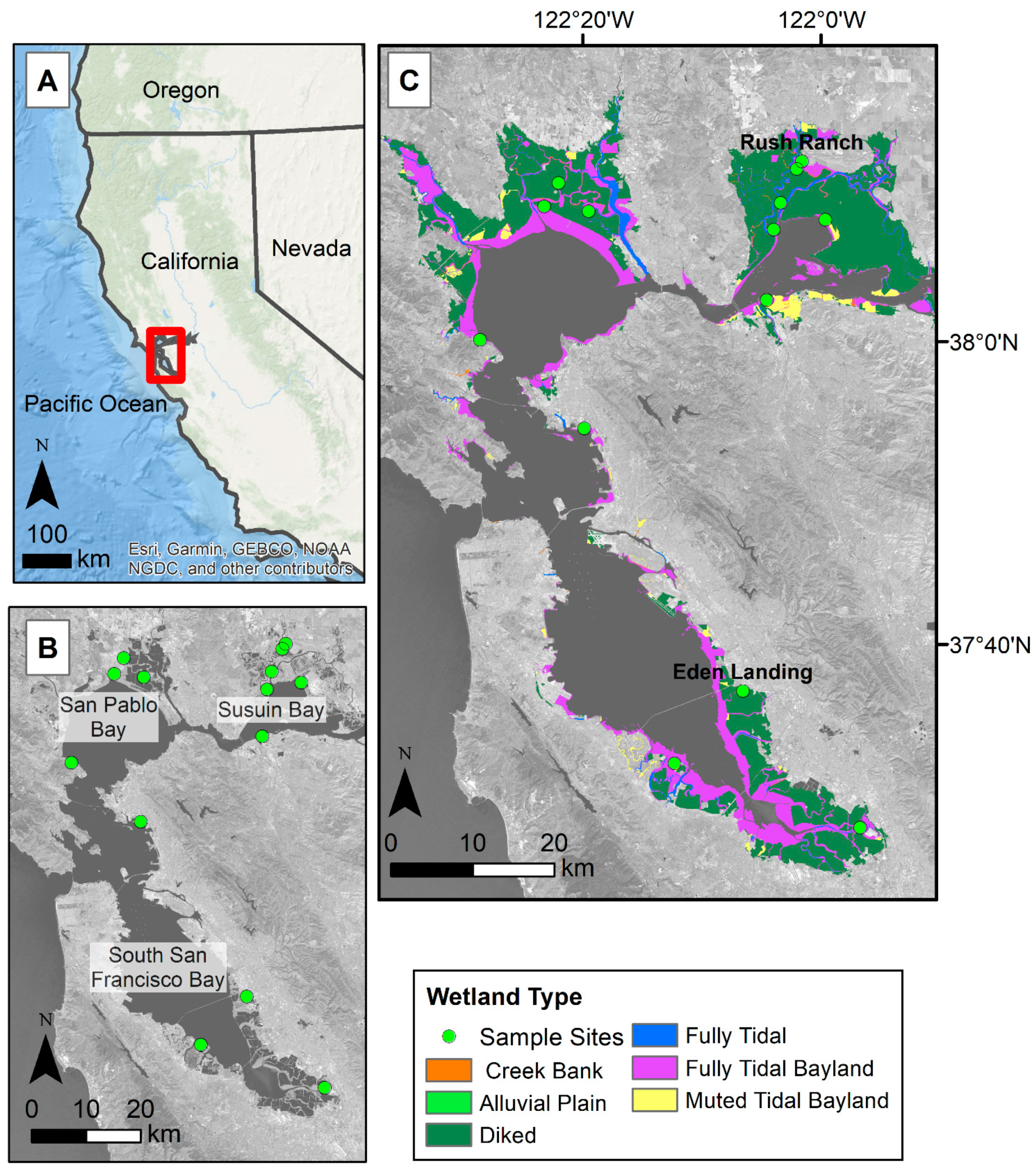
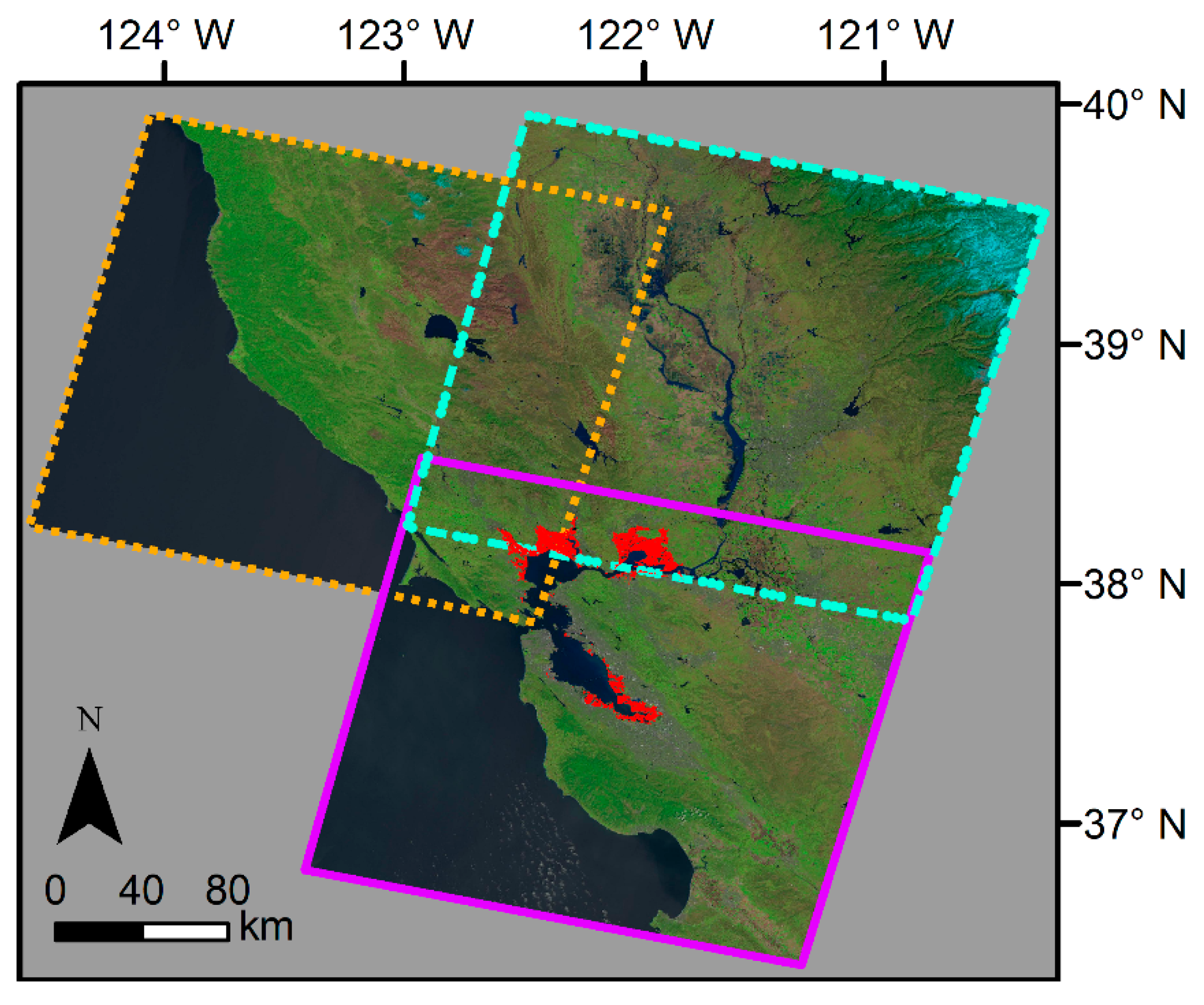
2.1. Study Area

The study focused on tidal wetlands within the San Francisco Bay Estuary (Bay Area) as defined by the San Francisco Estuary Institute (Figure 1C, [33]). The study area was also constrained by the elevation dataset we used, which only includes salt and brackish tidal marshes within the Bay Area [34]. The Bay Area can be broken up into three regions, South San Francisco Bay (South Bay), San Pablo Bay, and Suisun Bay (Figure 1B). For model training, we focused on 14 areas within the Bay Area tidal wetlands (Figure 1B). The areas were semi-randomly selected and distributed across the Bay Area within known tidal wetland locations. The Bay Area has a dry season roughly between May and October, with the majority of the precipitation occurring in December through February [35]. Most of the freshwater supply is from the Sacramento–San Joaquin River system and enters the Bay Area through the Suisun Bay; only 10% of freshwater flows from smaller streams and creeks such as the Coyote Creek in the South Bay. This makes the South Bay more saline than the Suisun Bay [36].
Due to the availability of eddy covariance flux tower data at two locations within our study area (Figure 1), we also compared flux tower-derived gross primary production with modeled plant greenness within Eden Landing Ecological Reserve (Eden Landing) and Rush Ranch Open Space Preserve (Rush Ranch). Eden Landing is located within the South Bay and is managed by the California Department of Fish and Wildlife. The site is part of the South Bay Salt Pond Restoration project, where restoration started in 2003 and aimed at restoring former industrial salt ponds to their more natural state. Restoration at Eden Landing was completed in 2008 and includes roughly 835 acres of tidal salt marsh. The dominant plant community is Sarcocornia pacifica, however, Spartina foliosa, algal mats, and other vegetation are also present. Rush Ranch is located within the Suisun Bay and is part of the National Estuarine Research Reserve system. Rush Ranch is one of the few undiked brackish tidal marshes in San Pablo Bay and the marsh remains relatively undisturbed. The plant community here is more diverse and is vegetated with plants such as Distichlis spicata, S. pacifica, Schoenoplectus americanus, and Lepidium latifolium.

2.2. Datasets

We used a variety of spatial datasets within this study (Table 1) to capture the potential precursors of wetland phenological dynamics and their regional variability. To select and classify wetland types, we used San Francisco Bay Area EcoAtlas Modern Baylands (Baylands) data (Figure 1C, [33]). The Baylands data are a shapefile containing wetlands within the Bay Area. The wetlands are further classified into different categories based on characteristics such as tidal influence, management, and elevation. This dataset allowed us to model the EVI within known tidal wetland areas and analyze if wetland type played a role in model error. To further test for model error, we used a habitat restoration dataset (Habitat Projects). The Habitat Projects dataset is a spatial dataset and includes restoration projects within California, with a focus on wetland and coastal ecosystems [37].
To estimate vegetation greenness, we used Landsat 8 (Landsat) surface reflectance time series data accessible via Google Earth Engine (GEE), the open-source, cloud-based, web-enabled applied programming interface for multi-scale geospatial analyses [40]. This 30-meter spatial resolution product includes data from 2013 to the present and is available as atmospherically corrected using Land Surface Reflectance Code (LaSRC; [41]). With the image Quality Assessment (QA) band, we further reduced image noise by masking out clouds (bit attribute 5) and shadows (bit attribute 3). We selected all Landsat scenes (Figure A1) within the study area between 2013 and 2019. To estimate plant greenness, we calculated the Enhanced Vegetation Index (EVI). The EVI is less sensitive to soil and oversaturation than the commonly used Normalized Difference Vegetation Index, and several researchers have successfully used the EVI in wetland settings [5,42,43,44]. We calculated the Enhanced Vegetation Index using the following equation:
EVI = 2.5 × (NIR − red)/(NIR + C1 × red − C2 × blue + L)
where NIR is the near infrared band, red is the red band, and blue is the blue band. To calculate EVI history, we subset the Landsat data between 2013 and 2018 and calculated the two-week EVI mean regardless of year. To do this within GEE, we forced all the years to be the same placeholder value, while keeping the month and day values as is. We then summarized the data by taking the mean EVI value within 14-day periods. This gave us 26 spatially explicit EVI mean values summarized from the historical dataset.
To help account for interannual variations in plant growth, we included temperature and drought variables in our model, also using datasets accessible via GEE (Table 1). Previous studies found that aboveground biomass and plant greenness linearly correspond to temperature [45]. Similarly, researchers found that drought, or Palmer Drought Severity Index (PDSI), and aboveground biomass within wetlands are linearly correlated [46]. For weather data, we used PRISM Climate Group’s Daily Spatial Climate Dataset data (which includes temperature) and used the PDSI provided through the GRIDMET Drought dataset [39,47]. PDSI values range from −10 to 10 where values less than 0 indicate drier than normal conditions and values more than 0 indicate wetter conditions. Larger magnitudes indicate higher dry or wet signals.
We used two elevation datasets for this study. The first digital elevation model (DEM) is a 10-meter spatial resolution dataset resampled to 30 meters to match Landsat resolution. The dataset is a composite of DEMs acquired by the United States Geological Survey and the Department of Water Resources and is referenced to elevations above NAVD88 [38]. The second elevation dataset is also a composite of elevation datasets derived mostly from LiDAR but is referenced to elevations above mean higher high water (MHHW) and has a spatial resolution of 5 meters resampled to the 30-meter resolution of Landsat [34]. Tidal range is not constant across the Bay Area; using elevations above MHHW is a way to account for this difference. It is also a better determinant of flooding duration and the tidal influence on vegetation. Furthermore, wetlands within the Suisun Bay region have experienced a large amount of land subsidence. This gives the wetlands a lower elevation above NAVD88 than other wetlands within the Bay Area. However, due to the influence of dikes and levees, these wetlands do not experience the same tidal flooding as another wetland at a similar elevation above NAVD88.

2.3. Model Building and Predicting

In Google Earth Engine, we created a point at each Landsat pixel within the 14 model development sites, giving us a total of 239 points. Within this point dataset, we attached the elevation data, EVI history, and the 2019 Landsat 8-derived EVI time series. We then found the PDSI and temperature data with dates that most closely matched the 2019 Landsat acquisitions dates and attached them to the point dataset. The data were then exported into the R statistical program where we built and tested a series of predictive linear models to estimate the EVI at each Landsat pixel within the study area. Given the lack of previous studies and novelty of this analysis, we chose a linear regression approach as the main framework due to its relative ease of interpretation and comparison of different predictors (their coefficients and contributions to the model), and more transparent model error structure and performance assessment than with more complex and less transparent algorithms. Please note that even though we used linear multi-variate regression, not all predictors were included in a linear form, some were transformed to quadratic functions based on their statistical distribution, model diagnostics, and/or physical interpretation. For example, day of year (DOY) was used as a non-linear term because solar radiation follows a non-linear trajectory during a growing season. We then compared the models using Akaike information criterion (AIC) analysis [48]. We built the model using the following variables, a subset of the variables, and/or a variable transformation:
EVI = β 0 + β 1 DOY + β 2 EVI h + β 3 PDSI + β 4 Temperature + β 5 Elevation
where DOY is day of year, EVIh is historically observed EVI, PDSI is Palmer Drought Severity Index, Temperature is minimum, maximum, or mean temperature (°C), and Elevation is elevation (cm) above NAVD88 or mean higher high water (cm). β0 is the intercept while β1 − β5 are the fitted model coefficients corresponding to the predictor variables.
Using the best fit model and climate variables from 2019, we created a modeled 2019 phenological envelope by using the upper and lower bounds of the 95% confidence interval around predictor variable coefficients. This gave us maximum and minimum expected EVI values for 2019 (Figure 2). We did this for both the 14 study areas and for the tidal wetlands within the entire Bay Area.
To assess model accuracy, we calculated the root mean square error (RMSE) and the modified Willmott’s index of agreement (dmod) for the 2019 mean modeled EVI values versus Landsat observed EVI values [49]. The modified Willmott’s index of agreement is a way to calculate model performance. Values range from 0 to 1, and 1 indicates a perfect model fit. This index improves upon the original Willmott’s index. We used 95 random validation points throughout the Bay Area to calculate RMSE and dmod. We generated random points in ArcGIS, extracted the Landsat observed EVI and the mean modeled EVI, then exported the data into R. We calculated the RMSE using the following formula:
RMSE = 1 n × ( EVI obs EVI mod ) 2
where n is the sample size, EVIobs is the Landsat observed EVI, and EVImod is the modeled mean EVI. We calculated dmod using methods outlined by [50].
We also estimated model error within the entire Bay Area based on the phenological envelopes. We found the mean difference between the predicted EVI values and observed EVI values obtained from Landsat in 2019. To calculate the difference, we took the Landsat observed EVI minus the predicted values and set the difference to zero if the observed EVI values fell within the 95% confidence interval, or the phenological envelope, of the predicted values. We calculated the difference for each available 2019 Landsat scene and found the mean difference by taking the average of the difference maps, giving us one spatial map of mean difference. This gave us one spatially explicit mean difference map.

2.4. Additional Satellites in EVI Histories

To test if increasing the number of satellites used for creating EVI history improved our results, we expanded our satellite imagery to include Landsat 7 and the Harmonized Sentinel-2 imagery. We used the same calibrated model described above but used a different EVI history input based on what satellite(s) were used to calculate the mean historical fortnight EVI.
Landsat 7 is available within GEE, while the Harmonized Sentinel-2 imagery currently is not. The Harmonized Sentinel-2 data are available on NASA’s website, atmospherically corrected and calibrated to match Landsat 8 in pixel resolution (30 m) and spectral response [41]. Downloading and uploading the Harmonized Sentinel-2 data must be done manually, therefore we did not include all available images. We selected 49 Harmonized Sentinel-2 images that had no or low cloud cover and focused on dates that had fewer Landsat scenes. We then calculated the mean historical EVI using the combination of Landsat 7 and Landsat 8 then an additional mean EVI history using Landsat 7, Landsat 8, and the Harmonized Sentinel-2 imagery. This gave us two additional EVI history datasets, allowing us to analyze if adding additional satellites to the historical datasets improved our original model using EVI history based on Landsat 8 only. Using the two additional EVI history datasets, we predicted the EVI for 2019 throughout the Bay Area and calculated the difference similarly as described above.

2.5. Eddy Covariance Flux Tower Data

Eddy covariance data were collected at Rush Ranch and Eden Landing following similar approaches which allowed for calculation of 30-min average fluxes of CO2 between the marsh and atmosphere at the ecosystem scale [51]. Each tower was equipped with an open path CO2 and H2O infrared gas analyzer (LI-7500A/RS, LI-COR, Lincoln, NE, USA) and a sonic anemometer (Windmaster Pro, Gill Instruments Ltd., Lymington, Hampshire, UK and CSAT3, Campbell Scientific, Logan, UT, USA for Eden Landing and Rush Ranch, respectively). The instruments were mounted at 4.3 m and 3.4 m above the marsh surface for Eden Landing and Rush Ranch, respectively. Instruments were mounted on the northwestern side of each tower as both sites have predominant wind from the west (~270°). Raw data were recorded at 20 Hz frequency and the high-frequency data were processed to half hourly fluxes using EddyPro, with a missing samples allowance of 10%. Data and metadata are publicly accessible on the AmeriFlux website (US-Edn and US-Srr; https://ameriflux.lbl.gov/). Tower footprints were calculated using the Kljun model [52,53]. Currently, Rush Ranch eddy covariance data are available for between 2013 and 2017 and Eden Landing eddy covariance data are available for between 2018 and 2020.
Partitioning of net ecosystem exchange (NEE) into gross primary productivity (GPP) and ecosystem respiration at Rush Ranch followed Knox et al. [54]. Partitioning of NEE at Eden Landing was performed using an artificial neural network with input variables of sensible and latent heat flux, water table height, date, and tidal difference (the change in water table height between each half hour).

2.6. PEPRMT GPP Model

We used EVI predictions from Rush Ranch and Eden Landing to run a simple light use efficiency model previously applied to restored wetlands in the Sacramento–San Joaquin River Delta (PEPRMT model; [5,7]). The model was parameterized using Rush Ranch GPP measurements in 2016 and then applied to Eden Landing 2019 in a validation exercise [7].

3. Results

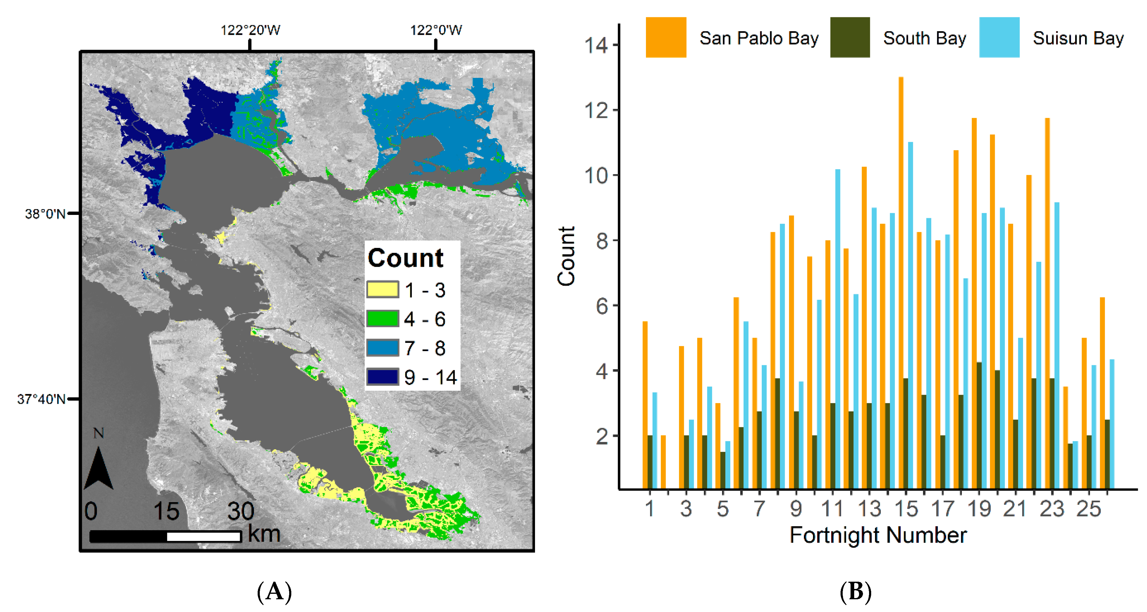
3.1. Satellite Image Count

The number of satellite images used for assessing the EVI history varied based on location within the Bay Area. Overall, the San Pablo Bay region had the highest image availability, and the South Bay had the fewest (Figure 3A). When factoring in the fortnight number, we further see that the South Bay consistently has the lowest number of available Landsat scenes (Figure 3B). There is also a seasonal pattern in available images, with the beginning and end of the year having the lowest image availability.

3.2. Model

Based on the model with the lowest AIC value (Table A1, dmod = 0.74), we found the following regression model to best predict the data:
EVI =   β 0 + β 1 DOY + β 2 DOY 2 + β 3 EVI h + β 4 PDSI + β 5 Tmin + β 6 MHHW + β 7 MHHW 2
DOY is the day of year, EVIh, is the EVI history, PDSI is the Palmer Drought Severity Index, Tmin is the minimum temperature (°C), and MHHW is elevation above mean higher high water (cm). The DOY and MHHW variables have a polynomial model fit. β0 represents the model intercept. Each subsequent β coefficient corresponds to the predictor variable. The β coefficients for each predictor vary based on if we are calculating the lower bound, mean, or upper bound EVI values (Table 2). Using the upper and lower bounds of the 95% confidence interval around the mean β coefficients, we modeled the 2019 EVI throughout the entire Bay Area tidal wetland landscape. This gave us 26 images of spatially explicit EVI envelopes, each representing a specific date range. Mean EVI values for the specific date range were also mapped, allowing for a spatial visual representation of plant greenness throughout the Bay Area for a given point in time (Figure 4). The summertime snapshot shows distinct areas of lower and higher plant greenness. The eastern portion of the San Pablo Bay has lower greenness than the rest of San Pablo Bay, the Suisun Bay has the overall highest greenness, while the South Bay has the lowest greenness.

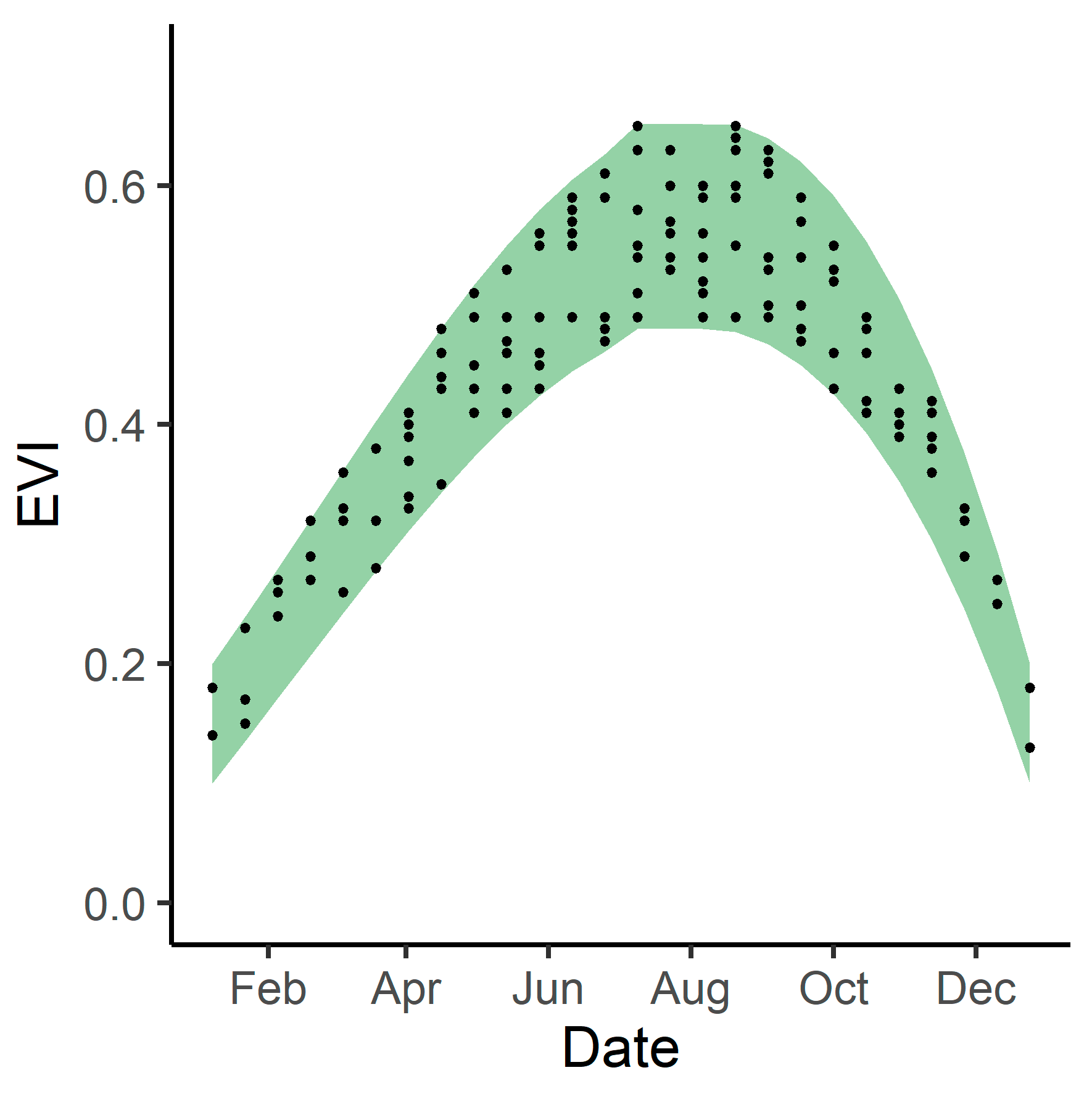
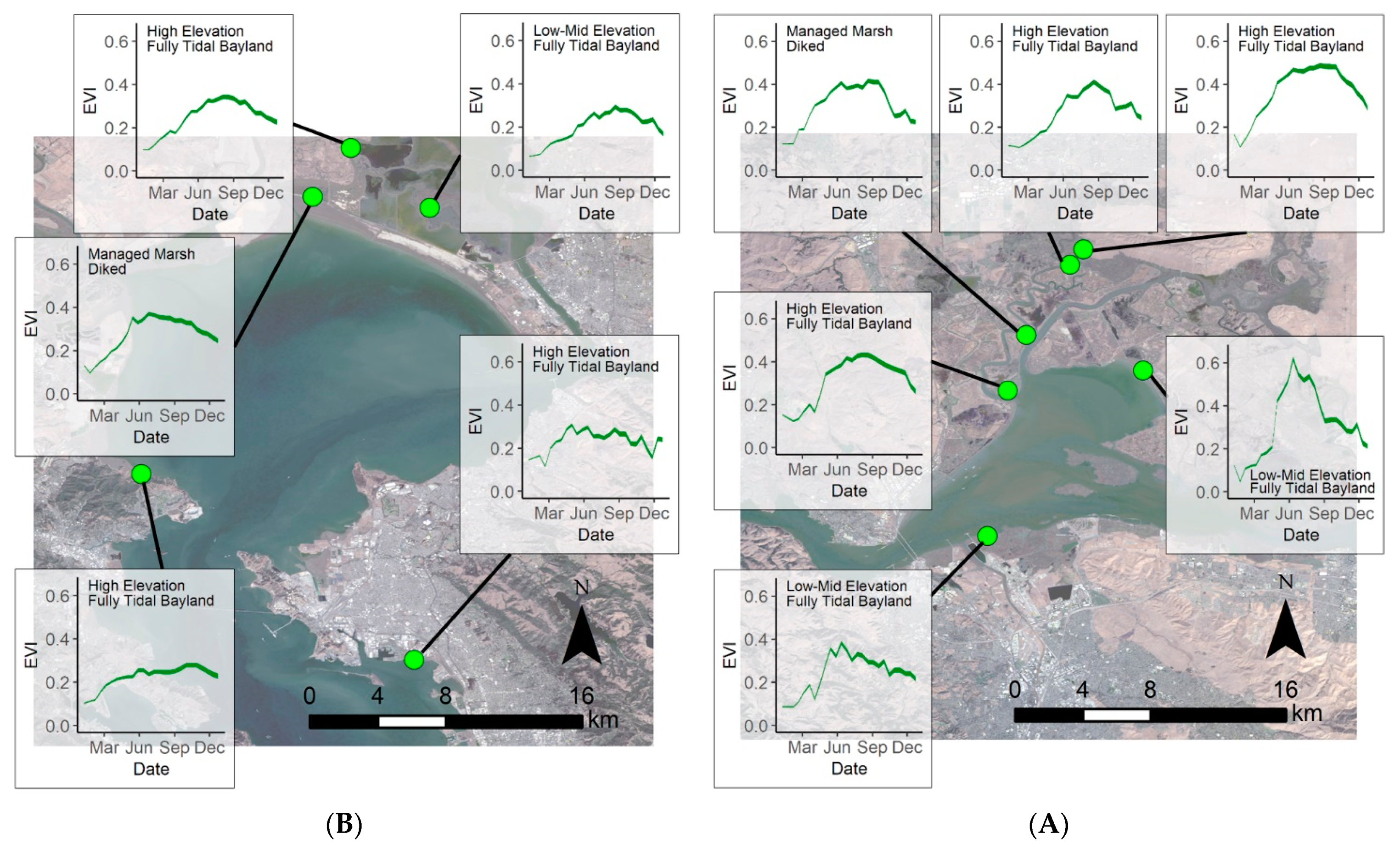
3.3. Phenological Envelope
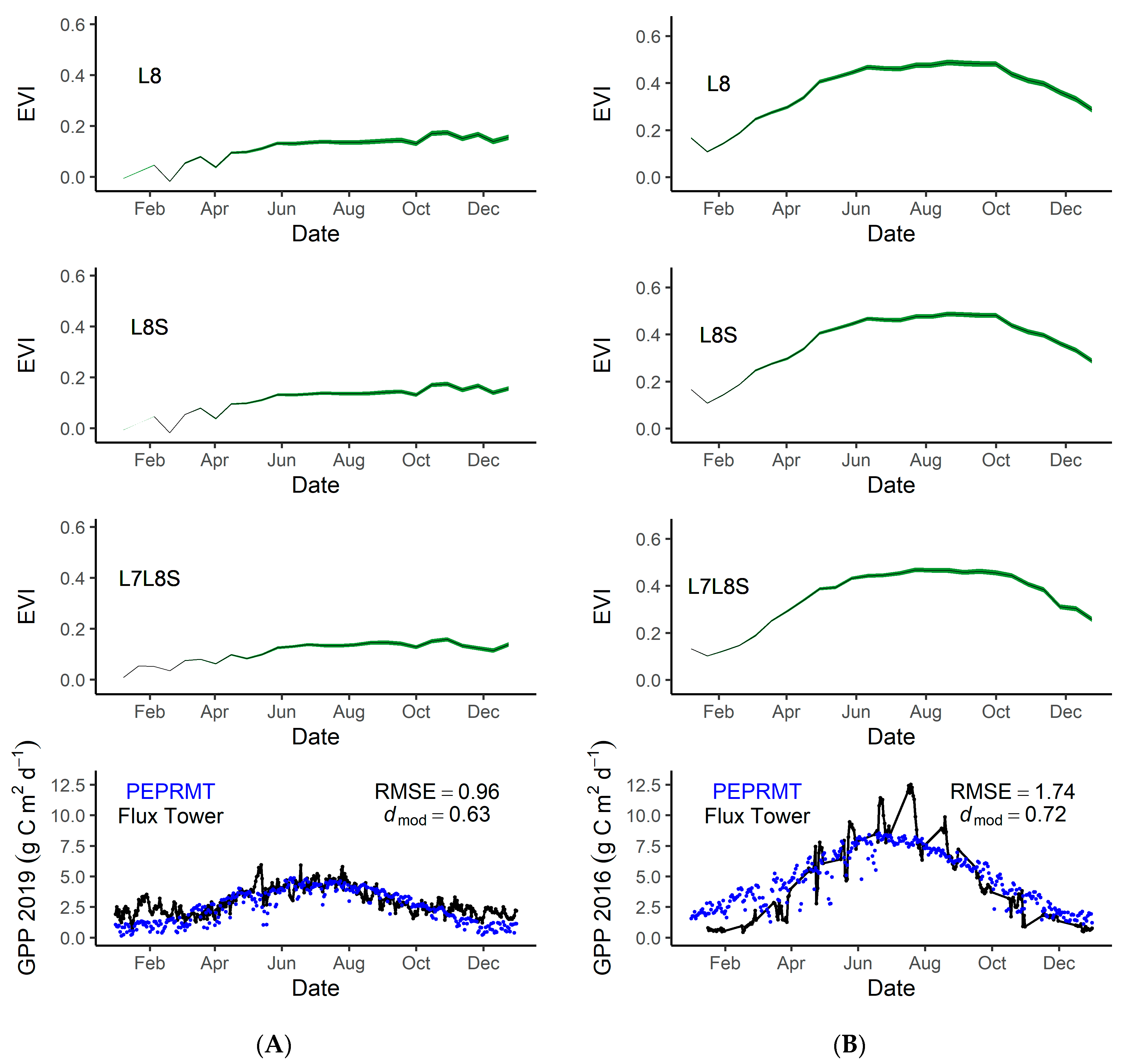
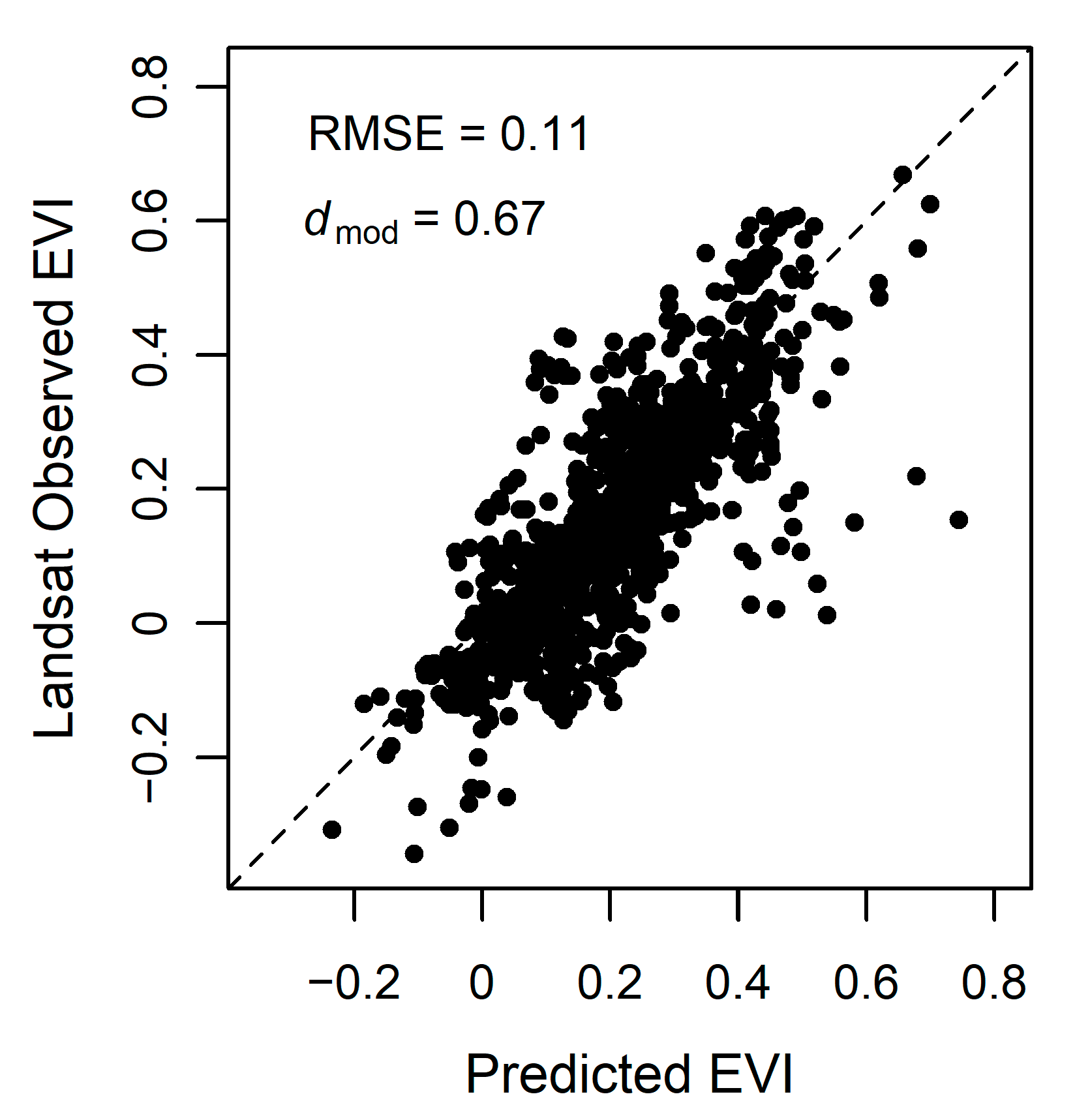
Extracting the EVI envelopes for each of the 14 model development sites, we determined the phenological curves capturing seasonal EVI variability for each site (Figure 5). This gave us the expected minimum and maximum EVI values throughout 2019 for each site. Phenological envelopes varied for each site, but overall sites had the lowest EVI during the winter with the EVI increasing in the spring, leveling off in the summer, then decreasing in the fall. Spatially, summer EVI values were highest in the Suisun Bay region (Figure 5A), lowest in the South Bay region (Figure 5C), and summer EVI values in the San Pablo Bay region (Figure 5B) were in between. Across these sites, the minimum modeled EVI was −0.02 and occurred in the winter while the maximum EVI was 0.63, occurring in summer.
Using the mean predicted EVI for Rush Ranch and Eden Landing, we ran a simple light use efficiency model (PEPRMT) [5,7] to test its ability to help improve predictions of GPP in tidal wetlands. We parameterized the model using 2016 data from Rush Ranch and validated the model using 2019 data from Eden Landing. Eddy covariance data was not available for 2019 within Rush Ranch, therefore we used 2016 data for GPP. Model performance was strong at Rush Ranch (dmod = 0.72, RMSE = 1.74; Figure 6B) and Eden Landing (dmod = 0.63, RMSE = 0.96; Figure 6A).

3.4. Model Accuracy

We assessed model accuracy both for validation points throughout the Bay Area and for tidal wetlands within the entire Bay Area. Model accuracy was high for the validation points; dmod = 0.67, RMSE = 0.11 (Figure 7). Throughout the Bay Area, the mean difference, or model error, varied but overall mean difference was low (Figure 8A). In general, the model tended to overestimate the EVI, with distinct areas of higher error within the San Pablo Bay region. When using EVI history that included Landsat 7 and Landsat 8 (EVIL7L8) or using the EVI history with Landsat 7, Landsat 8, and Harmonized Sentinel-2 (EVIL7L8Sent), we see minor differences within model error (Figure 6 and Figure 8). The EVI mean difference using EVIL7L8Sent history appears to be closer to zero (i.e., more yellow on the map, Figure 8A), indicating lower model error, with a few regions in the South Bay having higher model error (Figure 8A). Furthermore, the EVI envelopes have minor changes in shape when using multiple satellites to calculate EVI history versus using only Landsat 8 (Figure 6).
When summarizing model error within restoration project sites, we further see the highest model error within locations in the northwestern parts of the regions, i.e., San Pablo Bay (Figure A2B). For most restoration project sites, EVIs were overpredicted for 2019, while the averaged model error was −0.06 across the sites, the highest model over prediction was −0.213, and the highest model underprediction was 0.054. The areas with the highest model over- and underprediction were both located within the San Pablo Bay. A few small areas of underprediction also occurred within the Suisun Bay, while all the areas within the South Bay were overpredictions.
Comparing mean model error within bayland types and restoration projects, we further see that model error differs between types (Figure A4A). Overall restoration projects had the highest model error (~−0.057), muted tidal wetlands had the lowest (~−0.034), and all wetland types had an overprediction. When adding Harmonized Sentinel-2 to the Landsat 8 EVI history, there is little change within model error (Figure A4B). Restoration projects had the highest model error (~−0.057), and muted tidal wetlands had the lowest (~−0.034). When adding Harmonized Sentinel-2 and Landsat 7 to the Landsat 8 EVI history, model error significantly changes (Figure A4C). Restoration projects still had the largest error (~−0.054), and muted tidal wetlands had the lowest (~−0.023).
Model accuracy can also be influenced by tides and time since the end date of restoration. We analyzed model accuracy within the 14 model development locations and found the water level above mean higher high water observed during the Landsat image acquisition. This allowed us to determine that during the highest water levels, there was also higher calculated model error (Figure A5). We also examined how time since the end date of a restoration project was related to model error. The model restoration end date and model error were significantly correlated (Spearman correlation coefficient = −0.34), and model error was larger in areas with more recent restoration (Figure 9).

4. Discussion

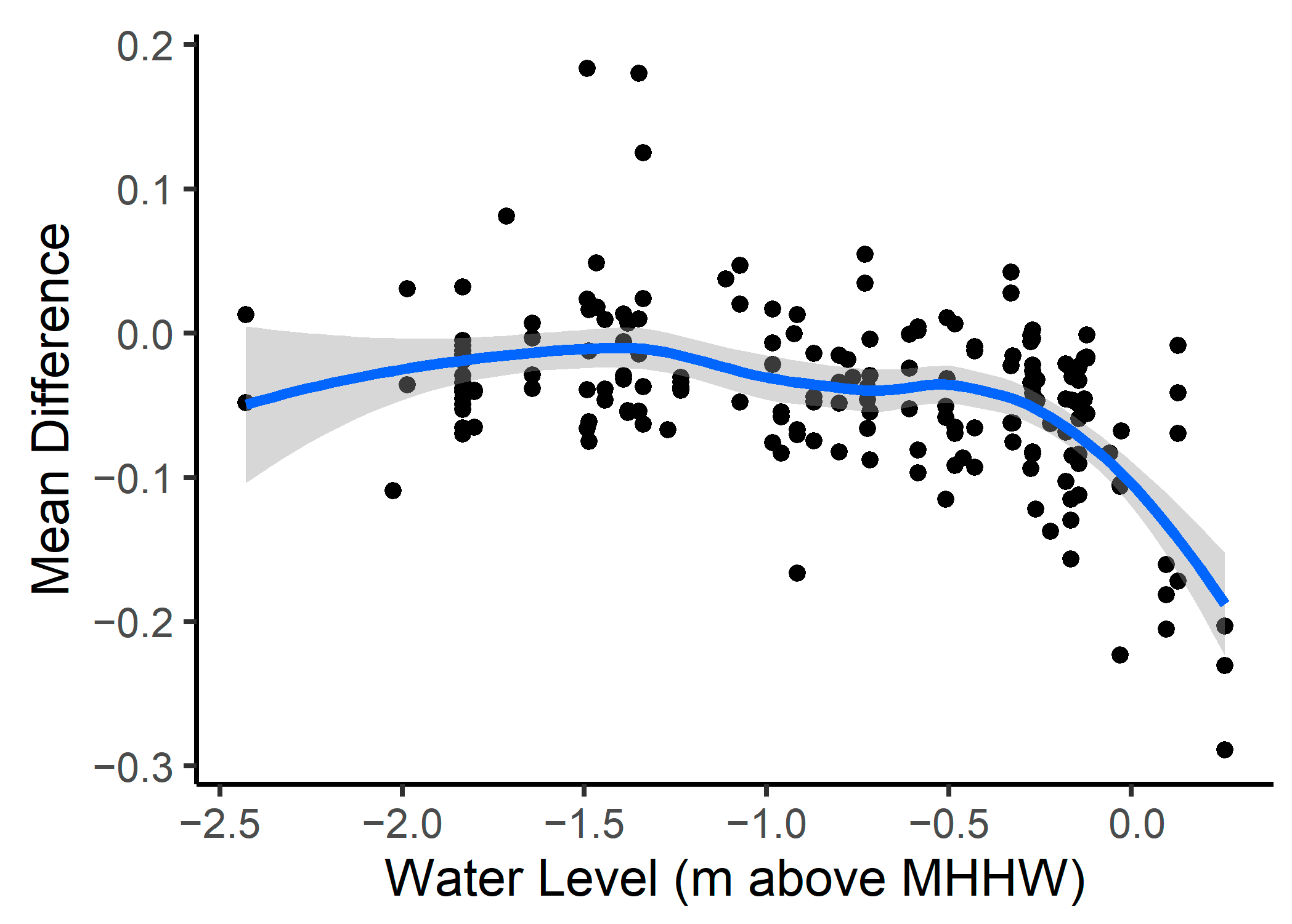
4.1. The Potential of Multi-Temporal Phenological Information to Facilitate Greenness Interpolation in Tidal Systems

Using historical EVI at given time steps in conjunction with elevation, temperature, and the Palmer Drought Severity Index, we were able to model minimum and maximum expected plant greenness, important inputs into greenhouse gas flux modeling, throughout an entire year. Remote sensing and particularly multi-spectral satellite data are useful tools in measuring plant greenness on a landscape scale and for establishing time series data capturing phenological dynamics of plant coverage and biomass. However, multi-spectral satellites cannot “see” through clouds, and within tidal wetlands, vegetation signals are influenced by tidal flooding as a function of elevation, tidal height, and vegetation height [14,25,26]. This makes it difficult to assess both the degree of flooding throughout the entire landscape at a given point in time, and the degree to which remotely sensed plant greenness is representative of the vegetation biomass at that time. Our modeling approach circumvented the need to consider tidal data as well as cloud-related limitations and the lack of repeated 3D assessments of vegetation at the landscape scale, allowing us to predict likely plant greenness. We also were able to obtain a full-season approximation of phenological variability (i.e., phenological envelopes), by estimating plant greenness throughout the entire year.
The historical two-week mean EVI values have the greatest importance in the model, indicated by the largest standardized beta coefficient. The Palmer Drought Severity Index has the second highest standardized beta coefficient and has the second largest influence on the model. This indicates that plant growth is dependent on drought conditions and the positive PDSI beta coefficient indicates that plant greenness is higher under wetter conditions. Other studies have also shown that tidal wetland plant growth decreases under years of drought [31,55]. With decreased rain, plants can experience higher stress through altered hydroperiod, reduced soil water availability and increased salt burden. The day of year beta coefficient has a negative squared polynomial term, meaning that EVI follows a concave parabolic relationship with DOY; the max EVI is in the middle of the year and the min is at the beginning and tail ends of the year. For minimum temperature, there is a negative beta coefficient, indicating that with warmer temperatures, the EVI is higher, reflecting the dynamics of plant biomass, photosynthetic activity, and metabolism following seasonal changes in solar radiation and atmospheric conditions. When looking at elevation above mean higher high water, there is a positive squared polynomial beta coefficient, indicating that the EVI follows a convex parabolic relationship with elevation.

4.2. Model Performance

We observed the highest model error within diked wetlands and restoration projects (Figure 8 and Figure 9). Diked wetlands are often highly managed for waterfowl, salt production, or agriculture, and thus their plant communities may not predictably respond to seasonal environmental conditions in their human-regulated state [56]. For example, the majority of the wetland areas within the Suisun Bay are managed by private Duck Clubs that control the tidal influence within the marsh and aim to grow food for waterfowl [57]. This manipulation of the landscape may lead to the larger model error. Within restoration project sites, we also see higher model error, which likely resulted from inter-annual transitions in vegetation coverage, biomass, and composition over the course of post-restoration plant colonization and re-establishment, making historical dynamics of greenness less representative of current phenology [31,32]. We also see high model error in four restoration projects within the San Pablo Bay region (Figure A2). Two of these projects were completed in 2009 and the other two were completed in 2015 (Figure A2). For the projects completed in 2015, the EVI history included values from before, during, and after the restoration project. The projects completed in 2009 and 2015 are likely still changing and revegetating. One of the restoration sites, the Napa-Sonoma Ponds 3, 4, 5, was formerly a salt pond with hypersaline conditions (Figure A3). It is possible that the system is still recovering and still approaching natural functioning observed in other similar wetlands. Furthermore, the elevation data from this site were collected in 2003 and have inevitably changed. Since elevation is a model parameter, the inaccurate elevation for this site may also be a factor in model error. To create a more accurate elevation map for restoration project sites, a more current LiDAR elevation could be used and converted to elevation above mean higher high water [21,27]. Since our study region is large, has different tidal regimes, and added complexity with diking, converting the more recent LiDAR dataset to elevation above mean higher high water across different types of wetlands and coastal structures was beyond the scope of our study. On a smaller scale of individual sites or management units, this could more feasible, and it would be useful for future research to dedicate efforts to create an accurate elevation and tidal inundation map within the Bay Area tidal wetlands.
Model performance slightly improved when using Landsat 7, Landsat 8, and Harmonized Sentinel-2 data to calculate the mean historical EVI dataset. This is evident by the overall lower model error when using these three datasets. We did not include all available Harmonized Sentinel-2 data since the dataset is not currently available on GEE and the process to add all available images is cumbersome, however, in the future the harmonized product may become available on GEE which would streamline the process. Another important thing to note about the Harmonized Sentinel-2 data is that the cloud mask is not optimal. We found that the cloud mask was often overly sensitive and removed sections within wetland areas that did not contain clouds. This is a noted issue within the Harmonized Landsat 8 Sentinel-2; and future work could be done to improve automation of cloud removal for the Harmonized Sentinel product [41].
Lastly, we estimated model performance by comparing the predicted EVI to the satellite observed EVI. As mentioned previously, remotely sensed plant greenness might not accurately represent actual greenness. This is especially concerning in tidal wetlands since flooding may completely or partially submerge vegetation. Since it is difficult to ensure that the satellites acquired imagery only during low tide (this may not always be possible at lower revisit frequencies), tidal height varies both throughout the different images and throughout the landscape. After accounting for tidal height in the 14 model development sites, we observed higher model error during the highest tides. In a portion of the satellite images, the vegetation signal is likely reduced by tidal influence. This indicates that actual model error might be lower than estimated.

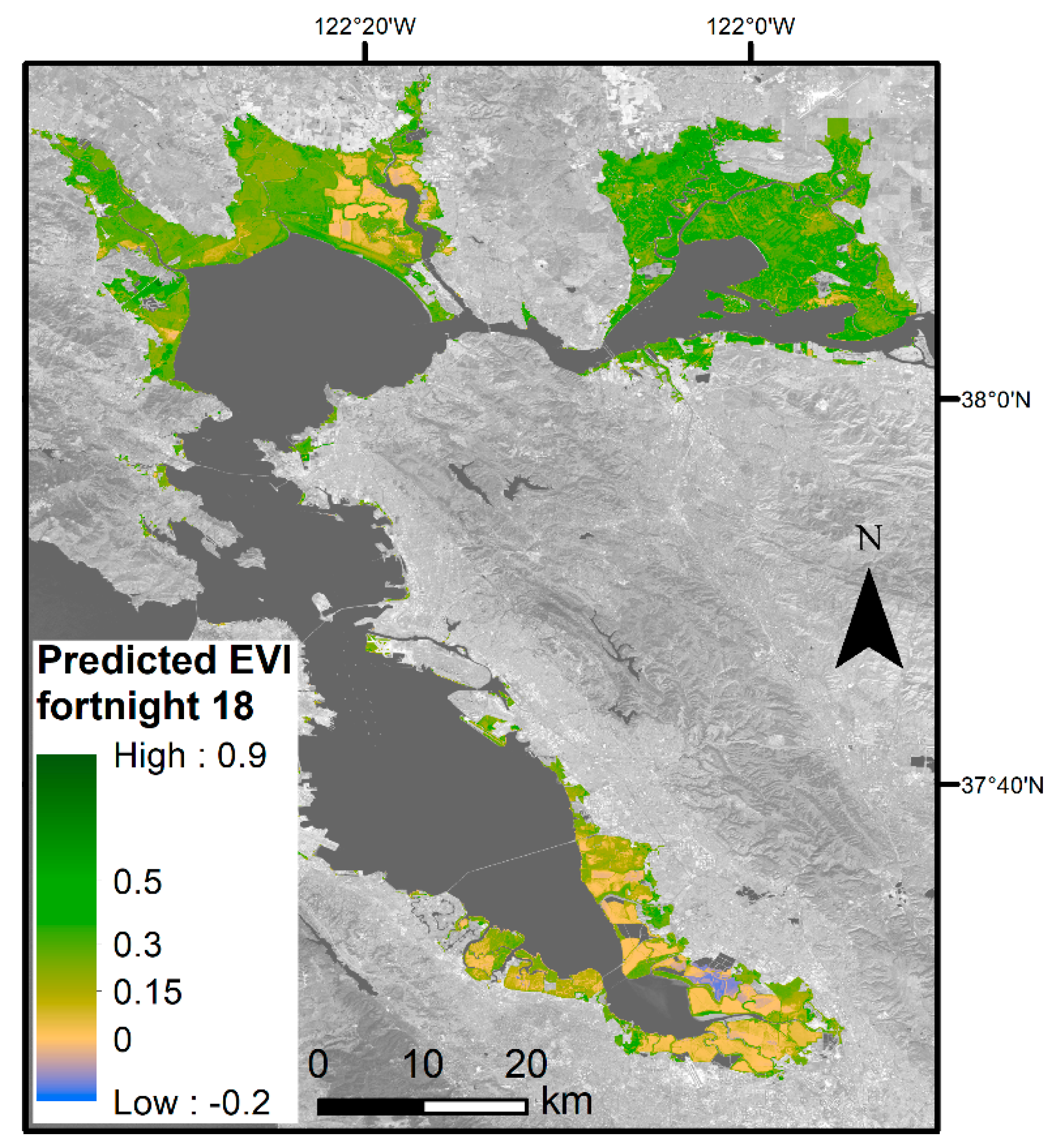
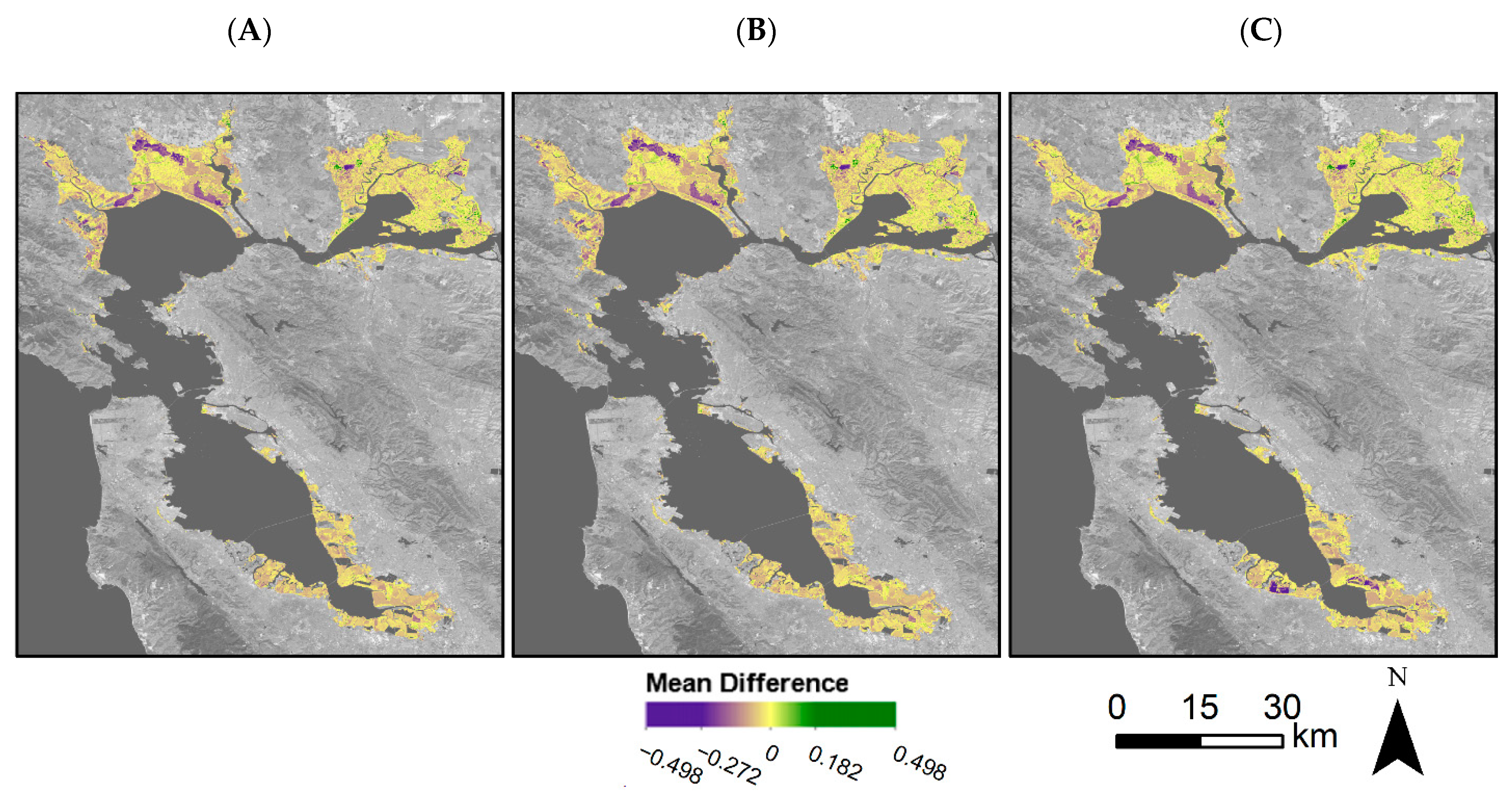
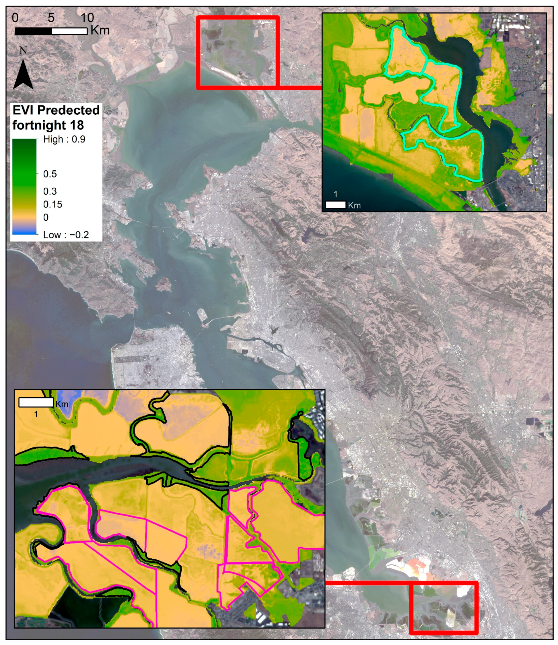
4.3. Vegetation Greenness throughout the Bay Area

There is also notable regional variation in greenness phenology across the study region, which becomes evident in the modeling outcomes and has important implications for modeling biogeochemical fluxes. During the summer, tidal wetlands within the Suisun Bay in general have higher plant greenness, or EVI, than the South Bay or the San Pablo Bay (Figure 5). Suisun Bay is fresher than San Pablo Bay and South Bay due to freshwater inputs from the Sacramento and San Joaquin Rivers. Salinity stress can decrease plant growth rates while not impacting the photosynthetic rates, and this would lead to lower plant greenness of the same species and minimal difference in observed CO2 flux [58]. Salinity also helps dictate the vegetation assemblage. Byrd et al. also found that the Suisun Bay region has higher aboveground biomass within tidal wetlands than San Pablo Bay [24]. Though we did not estimate aboveground biomass, plant greenness and aboveground biomass are often related [4,24,59]. The eastern portion of the San Pablo Bay region has lower plant greenness than the rest of the San Pablo Bay. This area was historically tidal marshes, converted into salt ponds and farms, and subsequently restored into tidal marshes again. Restoration projects are still ongoing within this area, but several projects were completed in the early 2000s. Though many restoration projects are complete within this area, the sites are likely still recovering. Similarly, a large portion of the tidal wetlands within the South Bay were converted into salt ponds. Restoration projects have restored part of the salt ponds back into tidal wetlands, however, industrial salt ponds remain within the area. The high salinity and management practices within the salt ponds make it difficult for plant growth, and typically only a narrow range of algae can grow in their hypersaline water [60].
Although there currently is no single consistent vegetation map product for the whole study region, information from existing mapping efforts and field studies (e.g., [31,61,62,63,64]) strongly suggests the role of varying composition of plant communities in the observed magnitude of greenness and its phenological patterns. The dominant vegetation type within many tidally controlled bay area wetlands is Sarcocornia pacifica, or pickleweed; and this is especially true within the South Bay. S. pacifica is a succulent and does not completely turn brown like other Bay Area tidal wetland plants such as Spartina folisosa, Pacific cordgrass [65]. In a study in Spain, researchers found that Sarcocornia fruticosa had peak aboveground biomass within the winter months, while belowground biomass peaked in the spring and summer [66]. This may be one reason why the greenness curve for Eden Landing does not appear to decrease at the end of the year. However, another study looked at aboveground biomass of S. pacifica (also known as Salicornia virginica) and separated the biomass between the woody and the green succulent part. They found the succulent fraction was highest in the summer and lowest in the winter [67]. The succulent portion of S. pacifica is the green fraction while the woody part is the older brown portion; and this would indicate that there is higher photosynthesis during the summer months than the winter months and thus a summer growth signal should be observed within satellite data. However, the study also mentions the high spatial and temporal variability in S. pacifica aboveground biomass observed in other studies [67]. Furthermore, the greenness signal within Eden Landing, and other wetlands within the South Bay, is lower than wetlands in San Pablo Bay and Suisun Bay, making it more difficult to decipher a greenness curve. This is further compounded by algal films that are sometimes present within the area, further skewing the signal from the plants [31,65].

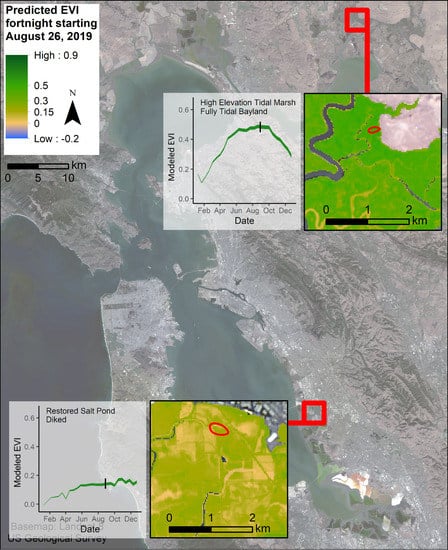
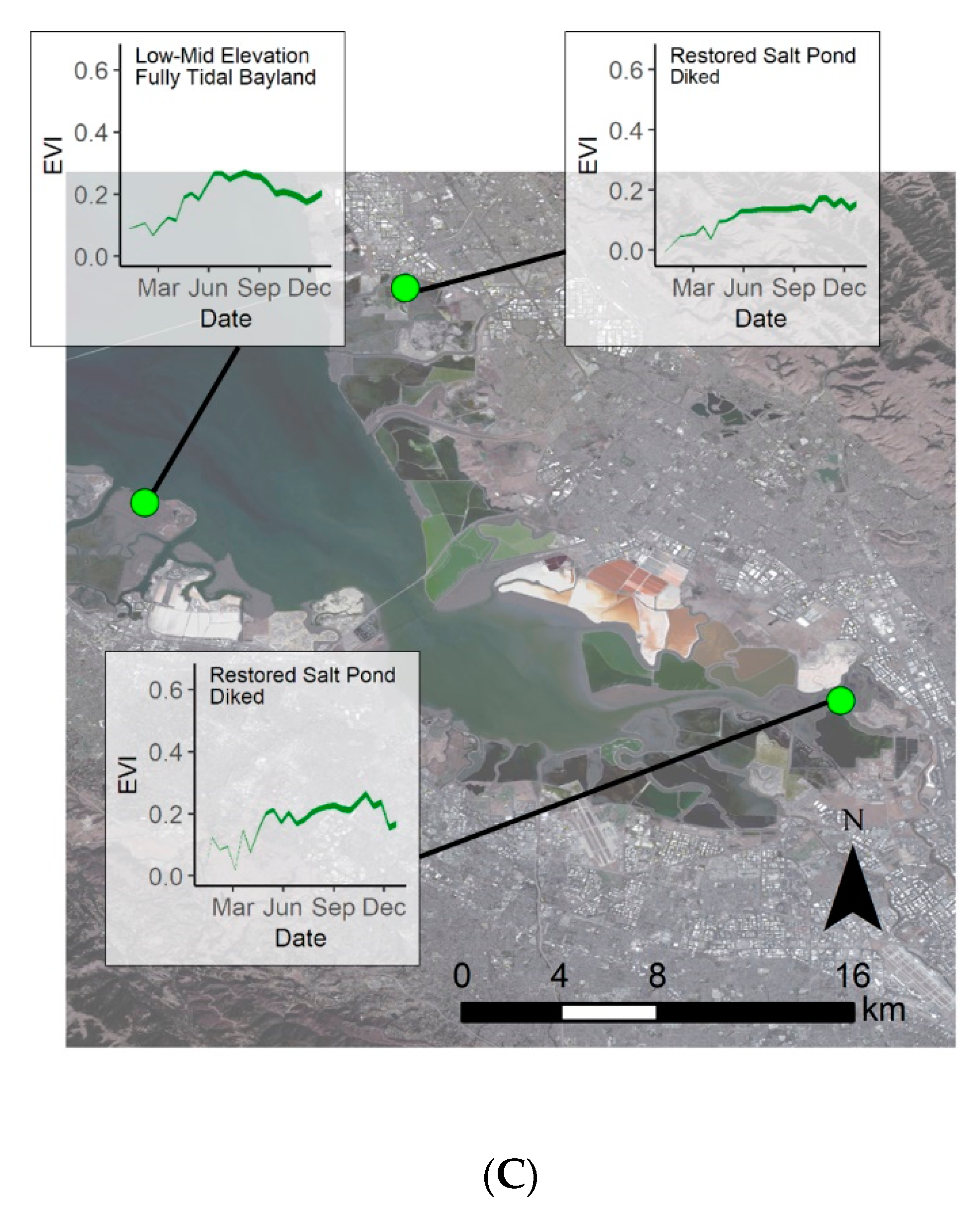
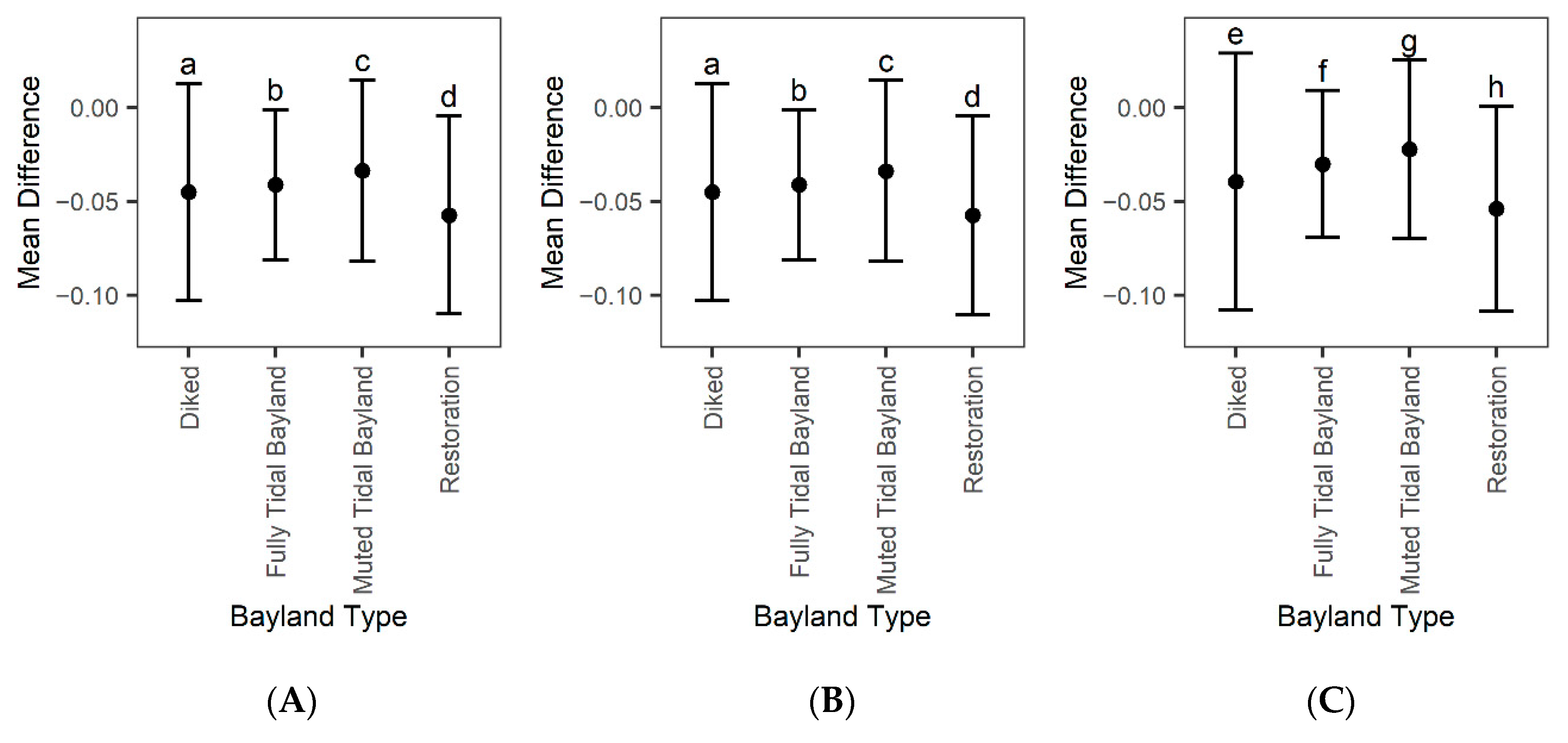
4.4. Restoration Areas

Given the varying and often uncertain time scales of wetland restoration projects before equilibrium stages [68], it is possible that the restored wetland areas are not yet fully restored, and the extent and density of vegetation are increasing. There are unaltered tidal wetland areas located adjacent to these restored sites, and the unaltered wetlands have higher plant greenness values than the restored sites (Figure A3). Model error is variable between each of the different restoration project sites, but we do see a trend that older, more established restored sites have less model error than more recently restored sites. Restoration projects ending in roughly 2000 or earlier all have similar model error and projects that ended after 2000 have higher model error (Figure A2). Wetland areas within restoration projects should be further investigated to determine the time frame it takes for the system to recover, and how wetland type plays a role in recovery time, which remains an important question in restoration efforts globally [31,32,68].

4.5. GPP Modeling

Wetland plant greenness is an important input into carbon sequestration models such as PEPRMT. Pairing our method of modeling the EVI with PEPRMT will allow for landscape-scale analysis of carbon sequestration within tidal wetlands over a given time frame. We have demonstrated that using our modeled EVI within the PEPRMT model provides an accurate estimate of gross primary production. This approach allows researchers to upscale ecosystem function across a large landscape. Future work could enhance these predictions further by incorporating in situ phenological observations from cost-effective phenocams and integrating them with satellite data [5,6], which would require expanding the scope of phenocam monitoring in this region. Engaging phenocam data to improve broader-scale predictions of phenology as satellite-based greenness envelopes would be especially beneficial for wetland sites showing high uncertainty in EVI modeling, such as actively managed or recently restored wetlands.

4.6. Limitations and Future Research Directions

Several limitations encountered in this study provide useful insights on the future research directions for advancing the use of remotely sensed phenological information in tidal marsh ecosystem analyses. One notable challenge concerned the variable availability of cloud-free Landsat time series across the study area. Although most of our focal region fits within one Landsat scene (WRS-2 path 44, row 34, Figure A1), the number of “usable” Landsat observation dates highly varies due to regular influxes of fog from the Pacific Ocean and its uneven distribution across the San Francisco Bay region. The South Bay experiences more cloud cover than the Suisun Bay and San Pablo Bay, which reduced the number of usable images to quantify historical variability in the EVI for wetlands in this part of the region. In addition, two Landsat tiles covered most of the Suisun Bay, three tiles covered the western part of the San Pablo Bay, and one Landsat tile covered the South Bay (Figure A1). The low image availability, especially within the South Bay, makes it particularly difficult to estimate tidal wetland plant growth cycles without using modeling approaches such as the one outlined in this paper. When data are limited, including the Sentinel Landsat harmonized product can be beneficial. Currently, the harmonized product is not available on GEE, however, data can be manually uploaded and incorporated into the EVI history calculation. Since this product is not currently available on GEE, we did not use this approach for the main model, however, the ability to find and process large amounts of Landsat data within GEE makes it ideal for time series analysis. In the future, Sentinel Landsat harmonized data may become available within the GEE database, which will likely improve our modeling approach.
Another notable challenge concerns lower applicability of the historical EVI to current-year seasonality in sites that have undergone a recent perturbation, such as restoration. Restoration projects can drastically alter the tidal regime, plant assemblage, and plant density. If the historical EVI dataset includes data from pre-restoration, the EVI signal can greatly differ from that after completion of the restoration project. Furthermore, the landscape continues to change even after completion of the restoration and there is not a universal timeline for when the ecosystem reaches an equilibrium state. For areas within known restoration projects, there is little to be done to improve our modeling approach, although this issue underscores an important and widely recognized research need to better understand the time frame of project dynamics, recoveries, and equilibria [68,69]. However, a shorter EVI history can be used which would only include data after completion of restoration. For historical data, emerging time series analysis tools such as Landsat-based Detection of Trends in Disturbance and Recovery (LandTrendr) can also help to identify characteristic time frames of post-restoration perturbation and recovery [70,71].
Lastly, using our modeling approach, we did not consider less common rapid unpredictable environmental changes. California is fire prone, so it is possible that fires will rapidly alter vegetation within wetland areas. For example, within Southern California, a fire resulted in decreased plant greenness within S. pacifica dominated wetland; vegetation eventually re-established but on the order of years [72]. It is more obvious which wetland areas experience fires, however, another natural phenomenon that is less spatially predictable and would influence vegetation coverage is salt marsh dieback. Salt marsh dieback is most noted in Spartina alterniflora dominated wetlands, has been recorded in California marshes, and causes regions of vegetation to thin or completely die [73]. The region eventually revegetates but the cycle takes years. Factors such as salinity, elevation, and drought may play a role in the vulnerability of a marsh to experiencing salt marsh dieback, however, the phenomenon is unpredictable [74]. Salt marsh dieback and burned areas would cause a lower observed plant greenness signal than predicted within our model.
Satellite data can be further validated or gap-filled through ground-based information such as through phenocams. Phenocams are low-cost cameras set up in the field that continuously take multi-spectral images. The cameras are set up horizontally across the landscape, which differs from satellite images which capture data from above. A relationship between the phenocam data and the satellite data can be established, allowing for gaps to be filled within the satellite time series. Phenocams also do not cover as wide of an area as satellites, which makes it more difficult to monitor vegetation across a large landscape while using phenocam data alone [6,54,75]. However, more widely collected phenocam data could improve our modeling approach in the future or provide for better validation of the growth curve envelopes that we model with satellite-based data.

5. Conclusions

Using EVI history and site characteristics such as elevation, the Palmer Drought Severity Index, and temperature, we can estimate the two-week Enhanced Vegetation Index, a popular spectral indicator of plant greenness, across the landscape for a given year. This allows us to estimate an EVI times series without having to consider tidal flooding, vegetation type, or unavailable satellite data due to poor atmospheric conditions. It also provides a practical strategy to predict proxies of vegetation phenological changes for modeling of plant-driven ecosystem processes in complex tidally influenced estuarine environments in the absence of repeated LiDAR observations. At the same time, our predictive modeling approach is sensitive to factors impacting the representativeness of phenological history of current ecosystem dynamics, particularly time since restoration, where more recently restored wetland sites tend to have larger model error. However, even among such projects, the degree of error varied, indicating that both site and time since restoration are important parameters to consider. Within restoration projects sites, the type of restoration, plant assemblage, and location within the Bay Area may all be factors in restoration success and system establishment. Overall, our findings indicate that this modeling approach can streamline estimating a vegetation time series across a large spatial extent. The predicted EVI output can then be incorporated into additional models such as PEPRMT which estimates carbon sequestration within wetlands. Future research could develop strategies to alleviate some of the key detected uncertainties. This includes more explicitly assessing restoration and management effects on wetland phenological dynamics within the regional context. This would allow for incorporating the status of these human interventions into phenological modeling.

Author Contributions

Conceptualization, G.J.M., I.D., P.Y.O., S.H.K., L.W.-M.; methodology, G.J.M., I.D.; software, G.J.M.; validation, G.J.M.; formal analysis, G.J.M.; investigation, G.J.M., I.D., P.Y.O.; resources, P.Y.O., I.D.; data curation, G.J.M., I.D., E.S.-H., J.S.; writing—original draft preparation, G.J.M., I.D.; writing—review and editing, G.J.M., I.D., P.Y.O., S.H.K., L.W.-M., J.S.; visualization, G.J.M.; supervision, P.Y.O., I.D.; project administration, P.Y.O.; funding acquisition, P.Y.O. All authors have read and agreed to the published version of the manuscript.

Funding

This research was funded by California Delta Stewardship Grant W2096-402.

Data Availability Statement

R code and Google Earth Engine code we generated for this study are available through GitHub at https://github.com/gwen210/EVI_Envelope.git (accessed on 29 July 2021).

Acknowledgments

Any use of trade, firm, or product names is for descriptive purposes only and does not imply endorsement by the U.S. Government. Publication made possible in part by support from the Berkeley Research Impact Initiative (BRII) sponsored by the UC Berkeley Library.

Conflicts of Interest

The authors declare no conflict of interest.

Appendix A

Table A1. Models used to estimate EVI for 2019. The model with the lowest AIC value is considered the best fit model. The K value is the number of parameters within the model, and ΔAIC is the difference between the AIC value for the given model and the AIC value from the best fit model.
ModelVariablesKAICΔAIC
H24DOY+DOY2+EVIh+PDSI+Tmin+MHHW+MHHW29−201,9910
H14DOY+DOY2+EVIh+PDSI+Tmin+NAVD+NAVD29−201,94348
H25DOY+DOY2+EVIh+PDSI+Tmax+MHHW+MHHW29−201,887104
H15DOY+DOY2+EVIh+PDSI+Tmax+NAVD+NAVD29−201,861130
H11DOY+DOY2+EVIh+PDSI+Tmax+NAVD 8−201,859132
H19DOY+DOY2+EVIh+PDSI+Tmax+ 7−201,855136
H16DOY+DOY2+EVIh+PDSI+Tmax+MHHW 8−201,854137
H26DOY+DOY2+EVIh+PDSI+Tmean+MHHW+MHHW29−201,835156
H12DOY+DOY2+EVIh+PDSI+ NAVD 7−201,815176
H10DOY+DOY2+EVIh+PDSI+Tmean+NAVD 8−201,814176
H8DOY+DOY2+EVIh+PDSI+ NAVD+NAVD28−201,814177
H9DOY+DOY2+EVIh+PDSI+ 6−201,812179
H20DOY+ EVIh+PDSI+Tmin+NAVD+NAVD28−201,453537
H17 EVIh+PDSI+Tmin+NAVD 6−201,437554
H18DOY+DOY2+EVIm+PDSI+Tmax+NAVD+NAVD29−198,5923399
H23DOY+DOY2+EVIm+PDSI+Tmax+MHHW+MHHW29−198,5573434
H7 EVIh+ Tmax 6−196,3285662
H21DOY+DOY2+EVIh+PDSI+Tmax+log(NAVD) 7−196,3275664
H4DOY+DOY2+EVIh+ NAVD 6−196,3265664
H22DOY+DOY2+EVIh+PDSI+Tmax+√NAVD 7−196,3265665
H3DOY+DOY2+EVIh+ 5−196,3245667
H6DOY+DOY2+EVIh+ Tmax 6−196,3225669
H2DOY+ EVIh+ 4−196,0875904
H13DOY+DOY2+EVIh+PDSI+ NAVD 6−93,559108,432
H5DOY+DOY2+ PDSI+Tmin+MHHW+MHHW28−93,360108,631
H1DOY+DOY2 4−92,126109,865
H0 2−76,636125,355

Appendix B

Figure A1. The three Landsat tiles that overlap our study area. Bay Area wetlands are highlighted in red. The main Landsat tile, WRS-2 path 44, row 34, is outlined in purple, while additional Landsat tiles that cover parts of San Pablo Bay and Suisun Bay are outlined in blue (WRS-2 path 45, row 33) and orange (WRS-2 path 44, row 33). Basemap: Landsat 8, U.S. Geological Survey.
Remotesensing 13 03589 g0a1
Figure A2. Model error (mean difference) within restoration project sites. Mean difference refers to the Landsat observed minus 2019 predicted EVI. We used a restoration project database obtained from EcoAtlas to calculate the mean difference within each site. (A) The mean difference averaged within the restoration project site. (B) End date of the restoration project, as obtained from EcoAtlas. The dates are binned into categories for easier visualization. Basemap: Landsat 8 band 7 (SWIR 2), U.S. Geological Survey.
Remotesensing 13 03589 g0a2

Appendix C

Figure A3. Zoomed in wetland areas within the South Bay and the Napa-Sonoma Ponds 3, 4, 5. Areas outlined in cyan are the Napa-Sonoma Ponds 3, 4, 5. The areas outlined in pink are restored wetland areas, and areas outlined in black are the historical wetland areas that have not been significantly altered. The blue to green shading indicates the predicted EVI for the fortnight starting 2 September 2018, with blue having the lowest plant signal and darker green the highest. Basemap: Landsat 8, U.S. Geological Survey.
Remotesensing 13 03589 g0a3

Appendix D

Figure A4. Mean difference (model error) plus or minus standard deviation based on bayland type. (A) Error based on modeling only using Landsat 8 for EVI history, (B) modeling including Landsat 8 and Sentinel for EVI history, and (C) Landsat 7 Landsat 8 and Sentinel for EVI history. Mean difference refers to predicted values minus 2019 Landsat observed data. Bayland type is defined by the San Francisco Estuary Institute’s Modern Bayland dataset. We compared the mean difference across the three panels; bayland type errors with a different letter code are significantly different from each other based on Tukey’s HSD.
Remotesensing 13 03589 g0a4

Appendix E

Figure A5. Model error (mean difference) versus water level (m) above MHHW. Mean difference is the predicted EVI minus 2019 observed Landsat EVI. We estimated the water level by finding the water level at the tide gauge closest to the study sites used for model development. We only calculated the mean difference versus water level for the 14 study areas used for model development. We found the mean difference versus water level for all the available 2019 Landsat images. We fit a smoothing trendline with standard error to better understand how mean difference is influenced by water level.
Remotesensing 13 03589 g0a5

References

  1. Xiao, J.; Chevallier, F.; Gomez, C.; Guanter, L.; Hicke, J.A.; Huete, A.R.; Ichii, K.; Ni, W.; Pang, Y.; Rahman, A.F.; et al. Remote sensing of the terrestrial carbon cycle: A review of advances over 50 years. Remote Sens. Environ. 2019, 233, 111383. [Google Scholar] [CrossRef]
  2. McNicol, G.; Sturtevant, C.S.; Knox, S.H.; Dronova, I.; Baldocchi, D.D.; Silver, W.L. Effects of seasonality, transport pathway, and spatial structure on greenhouse gas fluxes in a restored wetland. Glob. Chang. Biol. 2017, 23, 2768–2782. [Google Scholar] [CrossRef] [PubMed] [Green Version]
  3. Anderson, F.E.; Bergamaschi, B.; Sturtevant, C.; Knox, S.; Hastings, L.; Windham-Myers, L.; Detto, M.; Hestir, E.L.; Drexler, J.; Miller, R.L.; et al. Variation of energy and carbon fluxes from a restored temperate freshwater wetland and implications for carbon market verification protocols. J. Geophys. Res. Biogeosci. 2016, 121, 777–795. [Google Scholar] [CrossRef]
  4. Wan, R.; Wang, P.; Wang, X.; Yao, X.; Dai, X. Mapping Aboveground Biomass of Four Typical Vegetation Types in the Poyang Lake Wetlands Based on Random Forest Modelling and Landsat Images. Front. Plant Sci. 2019, 1281. [Google Scholar] [CrossRef] [PubMed]
  5. Knox, S.H.; Dronova, I.; Sturtevant, C.; Oikawa, P.Y.; Matthes, J.H.; Verfaillie, J.; Baldocchi, D. Using digital camera and Landsat imagery with eddy covariance data to model gross primary production in restored wetlands. Agric. For. Meteorol. 2017, 237–238, 233–245. [Google Scholar] [CrossRef] [Green Version]
  6. Dronova, I.; Taddeo, S.; Hemes, K.S.; Knox, S.H.; Valach, A.; Oikawa, P.Y.; Kasak, K.; Baldocchi, D.D. Remotely sensed phenological heterogeneity of restored wetlands: Linking vegetation structure and function. Agric. For. Meteorol. 2021, 296, 108215. [Google Scholar] [CrossRef]
  7. Oikawa, P.Y.; Jenerette, G.D.; Knox, S.H.; Sturtevant, C.; Verfaillie, J.; Dronova, I.; Poindexter, C.M.; Eichelmann, E.; Baldocchi, D.D. Evaluation of a hierarchy of models reveals importance of substrate limitation for predicting carbon dioxide and methane exchange in restored wetlands. J. Geophys. Res. Biogeosci. 2017, 122, 145–167. [Google Scholar] [CrossRef]
  8. Keenan, T.F.; Baker, I.; Barr, A.; Ciais, P.; Davis, K.; Dietze, M.; Dragoni, D.; Gough, C.M.; Grant, R.; Hollinger, D.; et al. Terrestrial biosphere model performance for inter-annual variability of land-atmosphere CO2 exchange. Glob. Chang. Biol. 2012, 18, 1971–1987. [Google Scholar] [CrossRef]
  9. Keenan, T.F.; Gray, J.; Friedl, M.A.; Toomey, M.; Bohrer, G.; Hollinger, D.Y.; Munger, J.W.; O’Keefe, J.; Schmid, H.P.; Wing, I.S.; et al. Net carbon uptake has increased through warming-induced changes in temperate forest phenology. Nat. Clim. Chang. 2014, 4, 598–604. [Google Scholar] [CrossRef]
  10. Ramsey, E.W.; Laine, S.C. Comparison of landsat thematic mapper and high resolution photography to identify change in Complex Coastal Wetlands. J. Coast. Res. 1997, 13, 281–292. [Google Scholar]
  11. Ramsey, E.; Rangoonwala, A.; Chi, Z.; Jones, C.E.; Bannister, T. Marsh Dieback, loss, and recovery mapped with satellite optical, airborne polarimetric radar, and field data. Remote Sens. Environ. 2014, 152, 364–374. [Google Scholar] [CrossRef]
  12. Byrd, K.B.; O’Connell, J.L.; Di Tommaso, S.; Kelly, M. Evaluation of sensor types and environmental controls on mapping biomass of coastal marsh emergent vegetation. Remote Sens. Environ. 2014, 149, 166–180. [Google Scholar] [CrossRef]
  13. Mo, Y.; Momen, B.; Kearney, M.S. Quantifying moderate resolution remote sensing phenology of Louisiana coastal marshes. Ecol. Modell. 2015, 312, 191–199. [Google Scholar] [CrossRef]
  14. Kearney, M.S.; Stutzer, D.; Turpie, K.; Stevenson, J.C. The Effects of Tidal Inundation on the Reflectance Characteristics of Coastal Marsh Vegetation. J. Coast. Res. 2009, 256, 1177–1186. [Google Scholar] [CrossRef]
  15. Barr, J.G.; Fuentes, J.D.; Delonge, M.S.; O’Halloran, T.L.; Barr, D.; Zieman, J.C. Summertime influences of tidal energy advection on the surface energy balance in a mangrove forest. Biogeosciences 2013, 10, 501–511. [Google Scholar] [CrossRef] [Green Version]
  16. O’Connell, J.L.; Mishra, D.R.; Cotten, D.L.; Wang, L.; Alber, M. The Tidal Marsh Inundation Index (TMII): An inundation filter to flag flooded pixels and improve MODIS tidal marsh vegetation time-series analysis. Remote Sens. Environ. 2017, 201, 34–46. [Google Scholar] [CrossRef]
  17. Wedding, L.M.; Moritsch, M.; Verutes, G.; Arkema, K.; Hartge, E.; Reiblich, J.; Douglass, J.; Taylor, S.; Strong, A.L. Incorporating blue carbon sequestration benefits into sub-national climate policies. Glob. Environ. Chang. 2021, 69, 102206. [Google Scholar] [CrossRef]
  18. Sander, T.; Gerke, H.H.; Rogasik, H. Assessment of Chinese paddy-soil structure using X-ray computed tomography. Geoderma 2008, 145, 303–314. [Google Scholar] [CrossRef]
  19. Ramsey, E.; Nelson, G.; Baarnes, F.; Spell, R. Light Attenuation Profiling as an Indicator of Structural Changes in Coastal Marshes. In Remote Sensing and GIS Accuracy Assessment; Lunetta, R., Lyon, J., Eds.; CRC Press: New York, NY, USA, 2004; pp. 59–73. [Google Scholar]
  20. Ju, Y.; Hsu, W.C.; Radke, J.D.; Fourt, W.; Lang, W.; Hoes, O.; Foster, H.; Biging, G.S.; Schmidt-Poolman, M.; Neuhausler, R.; et al. Erratum to: Planning for the Change: Mapping Sea Level Rise and Storm Inundation in Sherman Island Using 3Di Hydrodynamic Model and LiDAR. In Seeing Cities through Big Data; Springer: Cham, Switzerland, 2017. [Google Scholar]
  21. Buffington, K.J.; Dugger, B.D.; Thorne, K.M.; Takekawa, J.Y. Statistical correction of lidar-derived digital elevation models with multispectral airborne imagery in tidal marshes. Remote Sens. Environ. 2016, 186, 616–625. [Google Scholar] [CrossRef] [Green Version]
  22. Thorne, K.; MacDonald, G.; Guntenspergen, G.; Ambrose, R.; Buffington, K.; Dugger, B.; Freeman, C.; Janousek, C.; Brown, L.; Rosencranz, J.; et al. U.S. Pacific coastal wetland resilience and vulnerability to sea-level rise. Sci. Adv. 2018, 4, eaao3270. [Google Scholar] [CrossRef] [Green Version]
  23. Rosso, P.H.; Ustin, S.L.; Hastings, A. Use of lidar to study changes associated with Spartina invasion in San Francisco Bay marshes. Remote Sens. Environ. 2006, 100, 295–306. [Google Scholar] [CrossRef]
  24. Byrd, K.B.; Ballanti, L.; Thomas, N.; Nguyen, D.; Holmquist, J.R.; Simard, M.; Windham-Myers, L. A remote sensing-based model of tidal marsh aboveground carbon stocks for the conterminous United States. ISPRS J. Photogramm. Remote Sens. 2018, 139, 255–271. [Google Scholar] [CrossRef]
  25. Miller, G.J.; Morris, J.T.; Wang, C. Estimating Aboveground Biomass and Its Spatial Distribution in Coastal Wetlands Utilizing Planet Multispectral Imagery. Remote Sens. 2019, 11, 2020. [Google Scholar] [CrossRef] [Green Version]
  26. Feagin, R.A.; Forbrich, I.; Huff, T.P.; Barr, J.G.; Ruiz-Plancarte, J.; Fuentes, J.D.; Najjar, R.G.; Vargas, R.; Vázquez-Lule, A.; Windham-Myers, L.; et al. Tidal Wetland Gross Primary Production Across the Continental United States, 2000–2019. Glob. Biogeochem. Cycles 2020, 34, e2019GB006349. [Google Scholar] [CrossRef]
  27. Buffington, K.J.; Dugger, B.D.; Thorne, K.M. Climate-related variation in plant peak biomass and growth phenology across Pacific Northwest tidal marshes. Estuar. Coast. Shelf Sci. 2018, 202, 212–221. [Google Scholar] [CrossRef]
  28. Forbrich, I.; Giblin, A.E.; Hopkinson, C.S. Constraining Marsh Carbon Budgets Using Long-Term C Burial and Contemporary Atmospheric CO2 Fluxes. J. Geophys. Res. Biogeosci. 2018, 123, 867–878. [Google Scholar] [CrossRef] [Green Version]
  29. Melaas, E.K.; Friedl, M.A.; Zhu, Z. Detecting interannual variation in deciduous broadleaf forest phenology using Landsat TM/ETM+ data. Remote Sens. Environ. 2013, 132, 176–185. [Google Scholar] [CrossRef]
  30. Melaas, E.K.; Sulla-Menashe, D.; Gray, J.M.; Black, T.A.; Morin, T.H.; Richardson, A.D.; Friedl, M.A. Multisite analysis of land surface phenology in North American temperate and boreal deciduous forests from Landsat. Remote Sens. Environ. 2016, 186, 452–464. [Google Scholar] [CrossRef]
  31. Chapple, D.; Dronova, I. Vegetation development in a tidal marsh restoration project during a historic drought: A remote sensing approach. Front. Mar. Sci. 2017, 4, 243. [Google Scholar] [CrossRef] [Green Version]
  32. Taddeo, S.; Dronova, I. Landscape metrics of post-restoration vegetation dynamics in wetland ecosystems. Landsc. Ecol. 2020, 35, 275–292. [Google Scholar] [CrossRef]
  33. SFEI. Bay Area EcoAtlas V1.50b4 1998: Geographic Information System of Wetland Habitats Past and Present. Available online: https://www.sfei.org/content/ecoatlas-version-150b4-1998#sthash.CycgJ0lr.dpbs (accessed on 10 December 2020).
  34. Stralberg, D.; Brennan, M.; Callaway, J.C.; Wood, J.K.; Schile, L.M.; Jongsomjit, D.; Kelly, M.; Parker, V.T.; Crooks, S. Evaluating Tidal Marsh Sustainability in the Face of Sea-Level Rise: A Hybrid Modeling Approach Applied to San Francisco Bay. PLoS ONE 2011, 6, e27388. [Google Scholar] [CrossRef] [Green Version]
  35. Conomos, T.J.; Smith, R.E.; Gartner, J.W. Environmental setting of San Francisco Bay. Hydrobiologia 1985, 129, 1–12. [Google Scholar] [CrossRef]
  36. MacWilliams, M.L.; Bever, A.J.; Foresman, E. 3-D simulations of the San Francisco estuary with subgrid bathymetry to explore long-term trends in salinity distribution and fish abundance. San Fr. Estuary Watershed Sci. 2016, 14, 2. [Google Scholar] [CrossRef] [Green Version]
  37. California Wetlands Monitoring Workgroup Habitat Projects. Available online: https://ecoatlas.org/regions/ecoregion/bay-delta (accessed on 21 June 2021).
  38. Wang, R.; Ateljevich, E.; Fregoso, T.A.; Jaffe, B.E. A Revised Continuous Surface Elevation Model for Modeling (Chapter 5). In Methodology for Flow and Salinity Estimates in the Sacramento-San Joaquin Delta and Suisun Marsh, 38th Annual Progress Report to the State Water Resources Control Board; California Department of Water Resources, Bay-Delta Office: Sacramento, CA, USA, 2018. [Google Scholar]
  39. Abatzoglou, J.T. Development of gridded surface meteorological data for ecological applications and modelling. Int. J. Climatol. 2013, 33, 121–131. [Google Scholar] [CrossRef]
  40. Gorelick, N.; Hancher, M.; Dixon, M.; Ilyushchenko, S.; Thau, D.; Moore, R. Google Earth Engine: Planetary-scale geospatial analysis for everyone. Remote Sens. Environ. 2017, 202, 18–27. [Google Scholar] [CrossRef]
  41. Claverie, M.; Ju, J.; Masek, J.G.; Dungan, J.L.; Vermote, E.F.; Roger, J.C.; Skakun, S.V.; Justice, C. The Harmonized Landsat and Sentinel-2 surface reflectance data set. Remote Sens. Environ. 2018, 219, 145–161. [Google Scholar] [CrossRef]
  42. Tan, Z.; Jiang, J. Spatial-temporal dynamics of wetland vegetation related to water level fluctuations in Poyang Lake, China. Water 2016, 8, 397. [Google Scholar] [CrossRef] [Green Version]
  43. Kang, X.; Hao, Y.; Cui, X.; Chen, H.; Huang, S.; Du, Y.; Li, W.; Kardol, P.; Xiao, X.; Cui, L. Variability and changes in climate, phenology, and gross primary production of an alpine wetland ecosystem. Remote Sens. 2016, 8, 391. [Google Scholar] [CrossRef] [Green Version]
  44. Huete, A.; Didan, K.; Miura, T.; Rodriguez, E.P.; Gao, X.; Ferreira, L.G. Overview of the radiometric and biophysical performance of the MODIS vegetation indices. Remote Sens. Environ. 2002, 83, 195–213. [Google Scholar] [CrossRef]
  45. Jiang, Y.; Tao, J.; Huang, Y.; Zhu, J.; Tian, L.; Zhang, Y. The spatial pattern of grassland aboveground biomass on Xizang Plateau and its climatic controls. J. Plant Ecol. 2015, 8, 30–40. [Google Scholar] [CrossRef] [Green Version]
  46. Mo, Y.U.; Kearney, M.; Momen, B. Drought-associated phenological changes of coastal marshes in Louisiana. Ecosphere 2017, 8, e01811. [Google Scholar] [CrossRef]
  47. Daly, C.; Halbleib, M.; Smith, J.I.; Gibson, W.P.; Doggett, M.K.; Taylor, G.H.; Curtis, J.; Pasteris, P.P. Physiographically sensitive mapping of climatological temperature and precipitation across the conterminous United States. Int. J. Climatol. 2008, 28, 2031–2064. [Google Scholar] [CrossRef]
  48. Burnham, K.P.; Anderson, D.R. Model Selection and Multimodel Inference: A Practical Information-Theoretic Approach; Springer Science & Business Media: New York, NY, USA, 2002; ISBN 0387953647. [Google Scholar]
  49. Willmott, C.J.; Ackleson, S.G.; Davis, R.E.; Feddema, J.J.; Klink, K.M.; Legates, D.R.; O’Donnell, J.; Rowe, C.M. Statistics for the evaluation and comparison of models. J. Geophys. Res. 1985, 90, 8995. [Google Scholar] [CrossRef] [Green Version]
  50. Pereira, H.R.; Meschiatti, M.C.; Pires, R.C.D.M.; Blain, G.C. On the performance of three indices of agreement: An easy-to-use r-code for calculating the willmott indices. Bragantia 2018, 77, 394–403. [Google Scholar] [CrossRef] [Green Version]
  51. Baldocchi, D.D. Assessing the eddy covariance technique for evaluating carbon dioxide exchange rates of ecosystems: Past, present and future. Glob. Chang. Biol. 2003, 9, 479–492. [Google Scholar] [CrossRef] [Green Version]
  52. Chu, H.; Luo, X.; Ouyang, Z.; Chan, W.S.; Dengel, S.; Biraud, S.C.; Torn, M.S.; Metzger, S.; Kumar, J.; Arain, M.A.; et al. Representativeness of Eddy-Covariance flux footprints for areas surrounding AmeriFlux sites. Agric. For. Meteorol. 2021, 301–302, 108350. [Google Scholar] [CrossRef]
  53. Kljun, N.; Calanca, P.; Rotach, M.W.; Schmid, H.P. A simple two-dimensional parameterisation for Flux Footprint Prediction (FFP). Geosci. Model. Dev. 2015, 8, 3695–3713. [Google Scholar] [CrossRef] [Green Version]
  54. Knox, S.H.; Windham-Myers, L.; Anderson, F.; Sturtevant, C.; Bergamaschi, B. Direct and Indirect Effects of Tides on Ecosystem-Scale CO2 Exchange in a Brackish Tidal Marsh in Northern California. J. Geophys. Res. Biogeosci. 2018, 123, 787–806. [Google Scholar] [CrossRef]
  55. Malone, S.L.; Starr, G.; Staudhammer, C.L.; Ryan, M.G. Effects of simulated drought on the carbon balance of Everglades short-hydroperiod marsh. Glob. Chang. Biol. 2013, 19, 2511–2523. [Google Scholar] [CrossRef] [PubMed]
  56. Jones, S.F.; Janousek, C.N.; Casazza, M.L.; Takekawa, J.Y.; Thorne, K.M. Seasonal impoundment alters patterns of tidal wetland plant diversity across spatial scales. Ecosphere 2021, 12, e03366. [Google Scholar] [CrossRef]
  57. Moyle, P.B.; Manfree, A.D.; Fiedler, P.L. Suisun Marsh: Ecological History and Possible Futures; University of California Press: Berkeley, CA, USA, 2014. [Google Scholar]
  58. Pearcy, R.W.; Ustin, S.L. Effects of salinity on growth and photosynthesis of three California tidal marsh species. Oecologia 1984, 62, 68–73. [Google Scholar] [CrossRef] [PubMed]
  59. Lumbierres, M.; Méndez, P.; Bustamante, J.; Soriguer, R.; Santamaría, L. Modeling Biomass Production in Seasonal Wetlands Using MODIS NDVI Land Surface Phenology. Remote Sens. 2017, 9, 392. [Google Scholar] [CrossRef] [Green Version]
  60. Takekawa, J.Y.; Lu, C.T.; Pratt, R.T. Avian communities in baylands and artificial salt evaporation ponds of the San Francisco Bay estuary. Hydrobiologia 2001, 466, 317–328. [Google Scholar] [CrossRef]
  61. Baye, P. Tidal Marsh Vegetation of China Camp, San Pablo Bay, California. San Fr. Estuary Watershed Sci. 2012, 10. [Google Scholar] [CrossRef]
  62. Boul, R.; Hickson, D.; Keeler-Wolf, T.; Jo, M.; Ougzin, A. 2015 Vegetation Map Update for Suisun Marsh, Solano County, California; California Department of Fish & Wildlife: Sacramento, CA, USA, 2018; p. 104.
  63. Khanna, S.; Santos, M.J.; Boyer, J.D.; Shapiro, K.D.; Bellvert, J.; Ustin, S.L. Water primrose invasion changes successional pathways in an estuarine ecosystem. Ecosphere 2018, 9, e02418. [Google Scholar] [CrossRef]
  64. McClure, A.; Liu, X.; Hines, E.; Ferner, M.C. Evaluation of Error Reduction Techniques on a LIDAR-Derived Salt Marsh Digital Elevation Model. J. Coast. Res. 2016, 32, 424–433. [Google Scholar] [CrossRef]
  65. Fulfrost, B. Habitat Evolution Mapping Project South Bay Salt Pond Restoration Project Final Report Habitat Evolution Mapping Project Final Report South Bay Salt Pond Restoration Project; Brian Fulfrost and Associates: Oakland, CA, USA, 2009. [Google Scholar]
  66. Curcó, A.; Ibàñez, C.; Day, J.W.; Prat, N. Net primary production and decomposition of salt marshes of the Ebre delta (Catalonia, Spain). Estuaries 2002, 25, 309–324. [Google Scholar] [CrossRef]
  67. Boyer, K.E.; Fong, P.; Vance, R.R.; Ambrose, R.F. Salicornia virginica in a Southern California salt marsh: Seasonal patterns and a nutrient-enrichment experiment. Wetlands 2001, 21, 315–326. [Google Scholar] [CrossRef]
  68. Moreno-Mateos, D.; Power, M.E.; Comín, F.A.; Yockteng, R. Structural and functional loss in restored wetland ecosystems. PLoS Biol. 2012, 10, e1001247. [Google Scholar] [CrossRef] [Green Version]
  69. Hemes, K.S.; Chamberlain, S.D.; Eichelmann, E.; Anthony, T.; Valach, A.; Kasak, K.; Szutu, D.; Verfaillie, J.; Silver, W.L.; Baldocchi, D.D. Assessing the carbon and climate benefit of restoring degraded agricultural peat soils to managed wetlands. Agric. For. Meteorol. 2019, 268, 202–214. [Google Scholar] [CrossRef]
  70. Kennedy, R.E.; Yang, Z.; Gorelick, N.; Braaten, J.; Cavalcante, L.; Cohen, W.B.; Healey, S. Implementation of the LandTrendr algorithm on Google Earth Engine. Remote Sens. 2018, 10, 691. [Google Scholar] [CrossRef] [Green Version]
  71. Kennedy, R.E.; Yang, Z.; Cohen, W.B. Detecting trends in forest disturbance and recovery using yearly Landsat time series: 1. LandTrendr—Temporal segmentation algorithms. Remote Sens. Environ. 2010, 114, 2897–2910. [Google Scholar] [CrossRef]
  72. Brown, L.N.; Rosencranz, J.A.; Willis, K.S.; Ambrose, R.F.; MacDonald, G.M. Multiple Stressors Influence Salt Marsh Recovery after a Spring Fire at Mugu Lagoon, CA. Wetlands 2020, 40, 757–769. [Google Scholar] [CrossRef] [Green Version]
  73. Neira, C.; Ae, L.A.L.; Grosholz, E.D.; Mendoza, G. Influence of invasive Spartina growth stages on associated macrofaunal communities. Biol. Invasions 2007, 9, 975–993. [Google Scholar] [CrossRef] [Green Version]
  74. Miller, G.J.; Morris, J.T.; Wang, C. Mapping salt marsh dieback and condition in South Carolina’s North Inlet-Winyah Bay National Estuarine Research Reserve using remote sensing. AIMS Environ. Sci. 2017, 4, 677–689. [Google Scholar] [CrossRef]
  75. Vrieling, A.; Meroni, M.; Darvishzadeh, R.; Skidmore, A.K.; Wang, T.; Zurita-Milla, R.; Oosterbeek, K.; O’Connor, B.; Paganini, M. Vegetation phenology from Sentinel-2 and field cameras for a Dutch barrier island. Remote Sens. Environ. 2018, 215, 517–529. [Google Scholar] [CrossRef]
Figure 1. Site map of larger study area and locations used for model development. (A) Red box indicates study area in relation to California, USA. (B) Areas with green dots show the locations used for model development. (C) Colored areas indicate the overall study area, and the different colors break up the wetlands by type as defined by the San Francisco Bay Area EcoAtlas Modern Baylands type [33]. Eden Landing and Rush Ranch sites shown in panel C are wetland sites with eddy covariance stations measuring greenhouse gas fluxes. Basemap images in panel B and C are Landsat 8 band 7 (SWIR 2), U.S. Geological Survey.
Remotesensing 13 03589 g001
Figure 2. Example of a phenological envelope (curve). The green shaded area represents the upper and lower bounds of expected EVI values, while the points indicate historical EVI values.
Remotesensing 13 03589 g002
Figure 3. Number of Landsat scenes used to generate EVI history. (A) The average number (count) of Landsat scenes used to generate average EVI history for each fortnight within the Bay Area. The numbers of scenes for each of the 26 fortnights were averaged together to generate one mean count map. Basemap: Landsat 8 band 7 (SWIR 2), U.S. Geological Survey. (B) Average number of Landsat scenes used within the 14 model development areas for each time step. The counts are further broken up into region, San Pablo Bay, South Bay, and Suisun Bay.
Remotesensing 13 03589 g003
Figure 4. Predicted mean EVI within Bay Area wetlands for fortnight number 18, which corresponds to the fortnight Scheme 26. 2019. Blue areas are likely flooded or not vegetated. Yellow areas are less vegetated and, as the color Table 8. band 7 (SWIR 2), U.S. Geological Survey.
Remotesensing 13 03589 g004
Figure 5. Modeled 2019 phenological envelopes at each of the 14 model development sites. (A) Represents the sites in San Pablo Bay, (B) the sites in Suisun Bay, and (C) the sites in South San Francisco Bay. Basemap: Landsat 8, U.S. Geological Survey.
Remotesensing 13 03589 g005aRemotesensing 13 03589 g005b
Figure 6. Top graphs are the 2019 predicted EVI values for Eden Landing (A) and Rush Ranch (B) using three different EVI history datasets. L8 indicates modeled EVI using Landsat 8 for EVI history, L8S indicates modeled EVI using Landsat 8 and Sentinel-2 for EVI history. L7L8S indicates modeled EVI using Landsat 7, Landsat 8, and Sentinel-2 for EVI history. The bottom graphs are eddy covariance measured gross primary production (GPP) at Eden Landing in 2019 (A) and Rush Ranch in 2016 (B). The green lines represent the predicted EVI values, the black dots and lines indicate the eddy covariance measured GPP, and the blue dots represent the PEPRMT modeled GPP. Eddy covariance data were not available for 2019 within Rush Ranch, therefore we used 2016 data. Root mean square error (RMSE) and modified Willmott’s index of agreement (dmod) for the observed versus predicted GPP are indicated in the figures.
Remotesensing 13 03589 g006
Figure 7. Predicted versus Landsat observed 2019 EVI from 95 random points throughout the Bay Area. The dashed line represents the 1:1 line of perfect agreement between predicted and observed values. Root mean square error (RMSE) = 0.11 and the modified Willmott’s index of agreement dmod = 0.67.
Remotesensing 13 03589 g007
Figure 8. Mean difference between predicted EVI and Landsat observed EVI for 2019 for (A) Landsat 8-derived EVI history, (B) Landsat 8- and Sentinel-derived EVI history, and (C) Landsat 7-, Landsat 8-, and Sentinel-derived EVI history. Mean difference refers to the Landsat observed minus predicted EVI values. Mean difference was set to zero if the observed values fell within the predicted 95% confidence interval, or the phenological envelope. The areas in purple indicate an overprediction in the model while areas in green indicate an underprediction in the model. Basemap: Landsat 8 band 7 (SWIR 2) U.S. Geological Survey.
Remotesensing 13 03589 g008
Figure 9. Restoration project end date versus mean difference. Mean difference is the model error calculated for Landsat observed minus predicted EVI. The project end dates for 128 restoration projects were obtained from EcoAtlas from their Habitat Projects dataset. A smoothing curve was fitted to the data using loess to estimate the trend within the data.
Remotesensing 13 03589 g009
Table 1. Datasets used to build the models and to further analyze model error.
Dataset NameDescriptionSourceTypeResolution
Elevation MHHWElevation above mean higher high water generated by Point Blue[34]Raster5 m
Elevation NAVD88Elevation above NAVD88 derived from various sources[38]Raster10 m
Atmospheric TemperatureGRIDMET: University of Idaho Gridded Surface Meteorological Dataset—daily temperature, including minimum, maximum, and mean temperature. Available on Google Earth Engine[39]Raster4 km
Palmer Drought Severity IndexGRIDMET DROUGHT: CONUS drought indices. Gridded biweekly PDSI based on the modified version of the Palmer Formula. Available on Google Earth Engine[39]Raster2.5 arc min
Landsat 8USGS Landsat 8 Surface Reflectance Tier 1. Available on Google Earth Engine Raster30 m
BaylandsSan Francisco Bay Area EcoAtlas Modern Baylands type[33]Shapefile
Habitat ProjectsLocations of restoration projects within San Francisco Bay Area Wetlands[37]Shapefile
Table 2. Model coefficients for the best fit model. The top value for each row represents the standardized and unstandardized β coefficients for each predictor variable of the best fit model. The lower two values of each line represent the lower and upper bounds of the 95% confidence interval around each coefficient.
Dependent VariablePredictorStandardized β Coefficient
[Lower Bound, Upper Bound]
β Coefficient
[Lower Bound, Upper Bound]
EVIIntercept *0.2353
[0.2346, 0.2361]
−2.672 e 03
[−4.23 e 03 , −1.11 e 03 ]
DOY *−0.0015
[−0.0018, −0.0011]
2.871 e 04
[2.62 e 04 , 3.13 e 04 ]
DOY2 *−0.0060
[−0.0065, −0.0055]
−7.420 e 07
[−8.05 e 07 , −6.79 e 07 ]
EVIh *0.1166
[0.1162, 0.1171]
1.002
[0.998, 1.005]
MHHW *−0.0008
[−0.0011, −0.0004]
2.836 e 05
[1.68 e 05 , 3.99 e 05 ]
MHHW2 *0.0014
[0.0010, 0.0018]
5.034 e 07
[3.65 e 07 , 6.42 e 07 ]
PDSI *0.0141
[0.0137, 0.0144]
7.563 e 03
[7.37 e 03 , 7.76 e 03
Tmin *−0.0035
[−0.0040, −0.0029]
−8.792 e 04
[−1.02 e 03 , −7.42 e 04 ]
Adjusted R2 = 0.8818. * p < 0.001.
Publisher’s Note: MDPI stays neutral with regard to jurisdictional claims in published maps and institutional affiliations.

