Article

Spatiotemporal Changes and Driving Factors of Cultivated Soil Organic Carbon in Northern China’s Typical Agro-Pastoral Ecotone in the Last 30 Years

1
School of Government, Heilongjiang University, Harbin 150080, China
2
Northeast Institute of Geography and Agroecology, Chinese Academy of Sciences, Changchun 130102, China
3
College of Public Administration and Law, Northeast Agricultural University, Harbin 150030, China
*
Author to whom correspondence should be addressed.
Remote Sens. 2021, 13(18), 3607; https://0-doi-org.brum.beds.ac.uk/10.3390/rs13183607
Submission received: 2 August 2021 / Revised: 30 August 2021 / Accepted: 6 September 2021 / Published: 10 September 2021
(This article belongs to the Special Issue Remote Sensing Applications in Agricultural Ecosystems)

Abstract

:
In order to explore the spatiotemporal changes and driving factors of soil organic carbon (SOC) in the agro-pastoral ecotone of northern China, we took Aohan banner, Chifeng City, Inner Mongolia Autonomous Region as the study area, used the random forest (RF) method to predict the SOC from 1989 to 2018, and the geographic detector method (GDM) was applied to analyze quantitatively the natural and anthropogenic factors that are affecting Aohan banner. The results indicated that: (1) After adding the terrain factors, the R2 and residual predictive deviation (RPD) of the RF model increased by 1.178 and 0.39%, with root mean square errors (RMSEs) of 1.42 g/kg and 1.05 g/kg, respectively; (2) The spatial distribution of SOC was higher in the south and lower in the north; the negative growth of SOC accounted for 55.923% of the total area, showing a trend of degradation; (3) Precipitation was the main driving factor of SOC spatial variation in the typical agro-pastoral ecotone of northern China, which was also affected by temperature, elevation, soil type and soil texture (p < 0.01). (4). Anthropogenic factors (carbon input and gross domestic product (GDP)) had a greater impact on SOC than did climate factors (temperature and precipitation), making anthropogenic factors the dominant factors affecting SOC temporal variation (p < 0.01). The results of this work constitute a basis for a regional assessment of the temporal evolution of organic carbon in the soil surface, which is a key tool for monitoring the sustainable development of agropastoral ecotones.

Graphical Abstract

1. Introduction

Soil is the largest carbon pool in terrestrial ecosystems, which plays an important role in monitoring and mitigating global environmental processes and maintaining agricultural systems’ stability [1]. SOC refers to humus, plant materials, animal residues and microorganisms formed by microorganisms in the soil matrix, which is an important index for soil fertility analysis, cultivated land quality evaluation and also an important soil indicator to ensure food security and sustainable agricultural development [2,3]. The accurate estimation of the soil carbon storage, as well as its spatio-temporal variation, is among key questions in the global carbon cycle and climate change research.
Since the 1970s, the rapid development of remote sensing technology has provided a new idea for SOC prediction. Compared with traditional methods, it can observe the ground on a large spatial scale and high temporal resolution. Soil spectral reflectance has a unique spectral response region to SOC, and the reflectance has a significant negative correlation with SOC [4]. Some studies have proven that visible near-infrared spectroscopy (450–880 nm) and shortwave infrared spectroscopy (1570–2290 nm) have good performance for SOC prediction [5,6,7]. Compared to hyperspectral images, multispectral images can record data in a wider wavelength range, which can reduce the inconsistency between wavelength and other data sources in the process of SOC prediction [8]. In addition, multispectral images can make long time-series analysis, and it is a low-cost and high-efficiency monitoring method. Grinand et al. [9] used Landsat images and environmental indices to predict SOC in humid and arid areas of Southeast Madagascar for 20 years, and the authors realized the monitoring of organic carbon storage on a landscape scale. Chen et al. [10] predicted the spatiotemporal variations in SOC in cultivated land of the Hubei Province by combining MODIS visible near-infrared bands and a vegetation index, mapping the 500 m × 500 m pixel SOC map from 2000 to 2017. As auxiliary data, multispectral optical remote sensing data have great potential in predicting the spatiotemporal distribution of SOC, while the impact of specific terrain factors on SOC prediction is still under exploration. For example, Yang et al. [11] combined regression kriging with distance to the ridge of mountains, relief degree of land surface, terrain wetness index, elevation and slope, obtaining an R2 of 0.66. Zhang et al. [12] found that the root mean square error (RMSE) decreased when the elevation was used as the auxiliary variable for SOC prediction.
RF is a regression model that combines the decision tree with bagging algorithms, and its strategy for selecting training samples can avoid over-fitting. Random Forest is a relatively new method for the spatial prediction of SOC concentrations and stocks [13]. Zeraatpisheh et al. [14] compared three different models to predict SOC: RF, Cubist (Cu), and Multiple liner regression (MLR). They concluded that RF has superior predictive capabilities on SOC prediction.
With the exploration of SOC prediction methods, scholars have also paid attention to the factors that affect the spatiotemporal variations in SOC. For example, terrain (e.g., elevation, slope, aspect) indirectly affects SOC through soil erosion and SOC mineralization [15]. Soil texture is remarkably conditioned by the soil parent material and is commonly the basis of the definition of “soil types”. It is also related to the spatial heterogeneity of the SOC, since it determines the contribution of the stabilized carbon within the finest fraction to the total organic carbon of the soil [16]. Temperature and precipitation indirectly affect the composition and turnover of SOC by directly affecting vegetation and microorganisms [17]. SOC was found to be negatively correlated with temperature and positively correlated with precipitation [18]. The chemical and biological availability of organic carbon input under different land-use patterns can control the formation of SOC [19]. Human activities directly affect the spatiotemporal changes in SOC by controlling the balance between carbon input and output. For example, Xie et al. [20] selected three typical cities in the Jiangsu Province as the study area and concluded that land-use change and carbon input played major roles in the spatiotemporal change in organic carbon. Zhao et al. [21] indicated that the increase in cultivated land organic carbon input in China from 1980 to 2011 was mainly controlled by economic and policy factors.
The agro-pastoral ecotone is a natural barrier for wind prevention and sand fixation and acts as a transition zone from semiarid areas to arid areas. It is also the best industrial area, integrating agriculture, forestry, and animal husbandry, but is also a typical ecologically vulnerable area. The agro-pastoral ecotone in northern China covers an area of approximately 100,000 km2, including nine administrative regions: Inner Mongolia Autonomous Region, Heilongjiang, Jilin, Liaoning, Hebei, Shanxi, Shaanxi, Gansu Provinces, and Ningxia Hui Autonomous Region. However, the special geographical location and topography of the agro-pastoral ecotone result in a cold and windy climate and poor gravel-sand characteristics [22]. A low SOC increases the uncertainty of SOC prediction. Some scholars have studied the agro-pastoral ecotone in China. Yao et al. [23] explored the response of organic carbon mineralization to vegetation restoration. Wang et al. [24] analyzed the spatiotemporal distribution of SOC by kriging interpolation methods and found that the reduction in SOC was affected by natural and anthropogenic activities. However, the analysis of SOC in the agro-pastoral ecotone by remote sensing technology is rare, and the degree of SOC driving factors still lacks quantitative research.
Taking a typical agro-pastoral ecotone as the study area, this paper used remote sensing technology to predict the spatiotemporal changes in SOC in the last 30 years and conducted a quantitative study of the driving factors of natural and anthropogenic activities. In the case of limited soil data, this study provides a new method for SOC time-series estimation and driving factor analysis. Therefore, the objectives of this paper were to (1) establish the SOC prediction model in northern China’s typical agro-pastoral ecotone; (2) explore the spatiotemporal changes in SOC from 1989 to 2018; (3) identify the driving factors on the spatiotemporal distribution and changes of SOC.

2. Materials and Methods
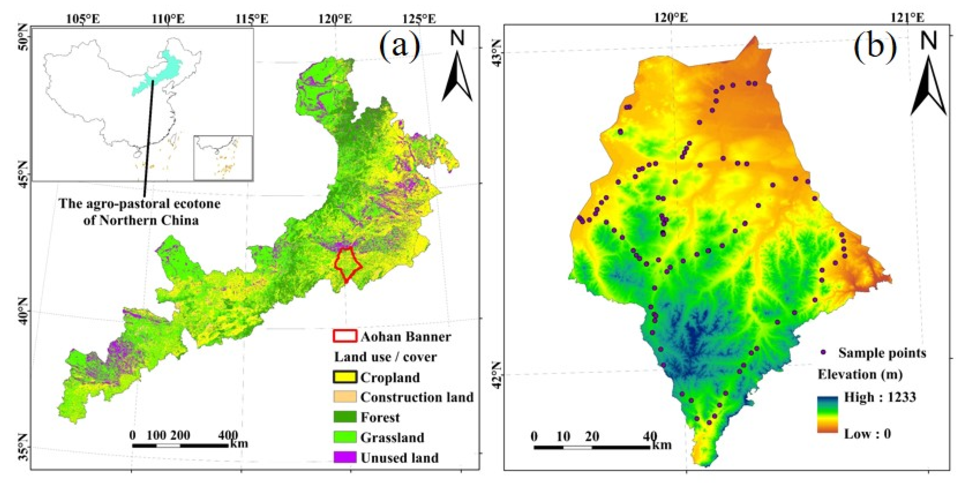
2.1. Study Area

The agro-pastoral ecotone of Northern China is a region of ecological transition between semi-humid cultivated cropping and arid/semiarid pastoral agriculture. This region contains sensitive terrestrial ecosystems vulnerable to climate change and human disturbance. Aohan Banner is a typical semiarid and agro-pastoral ecotone located in southeastern Chifeng city, Inner Mongolia Autonomous Region, China (Figure 1), with geographical locations of 41°69′~43°03′ and 119°53′~120°89′ and an area of 8316.2 km2. Aohan Banner is situated in the eastern part of the Yanshan Mountains, with the northern part located on the southern edge of Horqin sandy land, which is one of the four semiarid desert areas in China characterized by fixed, semi-fixed and mobile dunes. The southern part of Aohan Banner is mainly composed of cultivated land, woodland and grassland. It has a temperate continental monsoon climate according to the Köppen-Geiger climate classification system, with an annual precipitation of 374–524 mm and an average temperature of 6 °C. The average elevation is 517 m, but there is a large difference in terrain, with high elevation in the south and low elevation in the north. The cultivated land-use type is mainly dry land, and the main crops are corn and millet. Most crop straw in Aohan Banner can be returned to the field by machine. The “bare soil period” refers to the period when there is little crop residue and no snow cover in the fields, which is from mid-March to the end of April in Aohan Banner. Remote sensing images acquired during this period were not affected by straw, green crops or snow. Hence, this period was ideal for mapping the variability of soil properties [4].

2.2. Data Resources and Treatment

2.2.1. Soil Sample Collection and Treatment

In total, 102 soil surface (0–20 cm) samples were collected along the road in cultivated land by a manual soil auger on 14 May 2018. The location of soil samples was selected randomly according to prior knowledge with a five-point sampling method (for each soil sample, five soil subsamples including four corners and one center of a 1 m2 quadrat were mixed for one representative sample). The longitude and latitude information was recorded by GPS, and the soil samples were dried by the oven drying method [25] and then sieved by a 2 mm sieve. The SOC was determined by the potassium dichromate-volumetric method [26]. According to the classification of soil occurrence in China, we mainly collected four soil types: cinnamon soils, Castanozeras, gray fluvo-aquic soils and aeolian soils [27]. The SOC content in cinnamon soils is higher and its structure is looser, which makes the cinnamon soils more agronomically suitable than the other soil-types.

2.2.2. Image Acquisition and Treatment

Time-series analysis of SOC can be conducted with medium-high resolution remote sensing images, which are mostly commonly obtained from the Landsat satellite. The TM/ETM+ and OLI images from the Landsat satellite during four bare soil periods from 1989 to 2018 (Table 1) were obtained from https://glovis.usgs.gov/, (accessed on 25 March 2020) with the images free of cloud cover. There were some deviations in the acquired data due to the limitations of many factors, such as the spatial, temporal, spectral, radiation and resolution of the remote sensors, affecting the capture of complex land surface information. Thus, radiometric calibration, atmospheric correction (the result of atmospheric correction is the reflectance expanded by 10,000 times), mosaicking, and clipping of the images were conducted by ENVI5.3 (Exelis Inc., Boulder, CO, USA). Due to the arid climate, the average precipitation in March and April is approximately 0.30 mm, and the images selected in this study were taken during the bare soil period. Thus, the impact of precipitation and vegetation coverage on the images can be ignored. In addition, we obtained ETM+ on 18 March 2001 and on 25 March 2015, TM on 25 March 2001 and OLI on 17 March 2015 for cross-calibration. We selected 45 sample points, including water, vegetation and bare soil in the study area, and then extracted their reflectance from the Landsat images using the tool of extract multi values to points in ArcGIS 10.6. Because the operation period of ETM+ has an intersection with TM and OLI, we used ETM+ as a link to determine the cross-calibration coefficient of the three Landsat sensors to correct the TM sensors to the OLI level [28,29,30]. The results are shown in Table 2.

2.2.3. Acquisition and Treatment of Other Auxiliary Variables

Terrain is one of the most important soil forming factors in the arid and semi-arid regions. We obtained the 30 m digital elevation model (DEM) and extract maximum curvature (MaxC), minimum curvature (MinC) by ENVI 5.3 (Exelis Inc., Boulder, CO, USA) (Table 3), which were used as predictors on SOC prediction. DEM can also be used as one of the driving factors in the spatial variation analysis as well as clay, soil type, precipitation and temperature. The annual precipitation and annual temperature data were obtained from 1989 to 2018. We used kriging interpolation to obtain the spatiotemporal distribution of meteorological data in Aohan Banner.
The carbon input from 2000 to 2010 were estimated using net primary production (NPP) data. The NPP data were obtained from the Numerical Terra dynamic Simulation Group, which was used to represent human disturbance by controlling the balance of inputs. The gross domestic product from 1990 to 2010 was obtained from Resource and Environment Data Cloud Platform, Chinese Academy of Sciences, which can represent urban sprawl that is related to anthropogenic activities.
The cultivated land area data came from the National Earth System Science Data Center (http://www.geodata.cn/, accessed on 25 March 2020). The common cultivated land in the study period was selected as the scope of cultivated land.

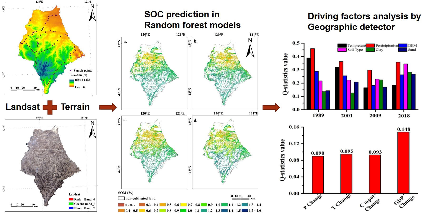
2.3. SOC Prediction Model

2.3.1. Random Forest (RF)

Random forest (RF) is a nonparametric method that consists of a large number of individual tree models trained from bootstrap samples of the data [31]. The number of optimal regression trees and the number of optimal splitting nodes are determined by out-of-bag data error. The final prediction value is the mean value of all tree models. The RF model can deal with high-dimensional data and has good robustness for feature selection. It has a high tolerance for outliers and noise and can thus effectively avoid the over-fitting phenomenon. It is a widely used machine-learning model [4,32]. In this paper, the RF package developed by Liaw and Wiener in R software (Version 3.6.1) was used to build the model, and mtree was set to 500. The default value of mtry is one-third of the total number of predictors, and there were seven input variables for prediction. Therefore, when mtry = 2, the out-of-bag error of these parameters will be more stable with maximized efficiency, which ranged from 0.06 to 0.08 in this study.
The 102 samples were randomly divided at a rate of 2:1 into a calibration set and a validation set. Then, we use the spectral reflectance, or adding terrain as variables in 2018 for modeling, and put the parameters extracted in 1989, 2001 and 2009 into the model to predict the SOC content in different time periods. See Section 3.5 for details.

2.3.2. Model Evaluation

The R2 and RMSE were used to evaluate the stability and accuracy of the model. The larger the R2 is, the higher the stability is; in contrast, the lower the RMSE is, the higher the accuracy is. The RPD (Residual predictive deviation) ≥ 2 indicates that the model has a very good prediction ability. If 1.4 ≤ RPD < 2, the model has good prediction ability, and if RPD < 1.4, the prediction ability of the model is not very good [4]. The corresponding formulas are given below:
R 2 = 1 i = 1 n ( y i y i ^ ) 2 i = 1 n ( y i y ¯ ) 2
RMSE = i = 1 n ( y i y i ^ ) 2 n
RPD = SD RMSE
Note: where n is the number of samples; y i is the observed SOC value of sample i ;   y i ^ is the predicted SOC of sample i; SD is the standard deviation of the predicted SOC value.

2.4. Geographical Detector Method (GDM) for Driving Factor Analysis

The GDM can be used to measure, exploit and analyze spatiotemporal heterogeneity. Now, it has been widely used to analyze the driving forces and multifactor interactions of various phenomena, including risk detection, factor detection, ecological detection and interaction detection [33]. We mainly used factor detection in this study. The core of this theory is to detect the consistency of spatial distribution patterns between dependent variables and independent variables through spatial heterogeneity and explain the contribution of independent variables to dependent variables, namely, the Q-statistics value [34]. The larger the Q-statistics value is, the stronger the contribution is. In this study, the driving factors of SOM are classified by the natural breakpoint method [34], and the driving factors are expressed quantitatively by the geographical detector method. The Q-statistic is calculated as follows:
q = 1 h = 1 L N h σ h 2 N σ 2
Note: q represents the Q-statistic value with a range value of (0, 1); L represents the number of strata; N and N h represent the total number of field samples and the number of samples in strata, respectively; σ 2 is the variance of the SOM in the study area. The GDM was executed with Geodetector software.

3. Results

3.1. Descriptive Statistics of the SOC

Descriptive statistical analysis is shown in Table 3. The SOC dataset of Aohan Banner ranged from 2.03 g/kg to 12.18 g/kg, which was lower than the average SOC content of the whole northern agro-pastoral ecotone in China [35]. In our study, the average SOC was 5.90 g/kg (Table 4), with a standard deviation (SD) of 2.11 g/kg and a coefficient of variation (CV) of 35.82%. A high SD and CV indicate that the SOC has strong spatial heterogeneity. The SOC content of the calibration set and validation set was evenly distributed, and the mean value was similar. Therefore, the sample of the calibration set and validation set was reasonable and representative.

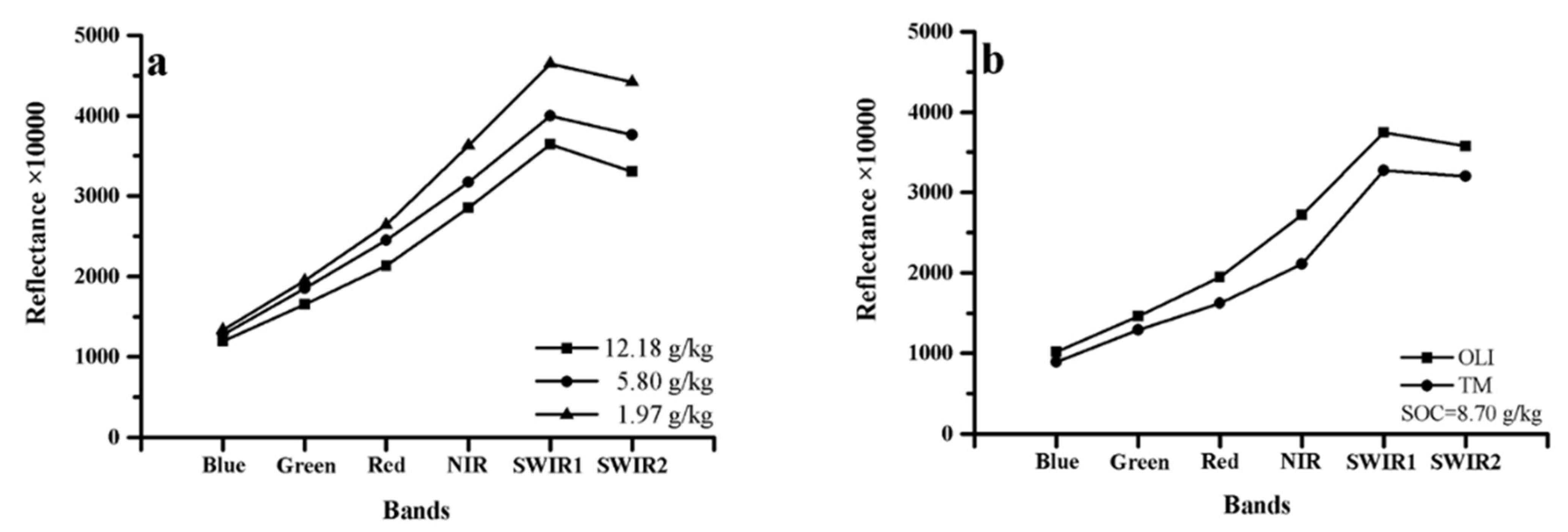
3.2. Reflectance Characteristics of Soil Samples

The maximum and minimum values of SOC samples were removed, and three representative samples were selected. The soil reflectance spectra of different SOC contents were extracted from the TM and OLI images (band 1~band 6 of TM corresponds to band 2~band 7 of OLI, respectively). The spectral reflectance decreases with increasing SOC content (Figure 2). In the visible spectrum, the soil reflectance spectra increase slowly with increasing wavelength, and the reflectance of the near-infrared and shortwave-infrared spectra increases faster with the maximum value occurring in the 6th band of OLI. The reflectance of TM was slightly lower than that of OLI, but the overall trend was consistent with OLI.

3.3. Selection of Predictors for SOC Prediction

According to the correlation analysis, four bands and three terrain factors with the highest correlations with SOC were selected as the input variables. The correlation coefficients are shown in Table 5. The results showed that the absolute value of the band correlation coefficient was higher than that of the terrain. The bands of OLI with a higher correlation with SOC were Band Red (−0.53), NIR (−0.60), SWIR1 (−0.64) and SWIR2 (−0.58). Elevation, MaxC and MinC had better correlations with SOC, and the correlations were 0.48, 0.48 and −0.48, respectively, indicating that SOC and terrain have a close relationship. We used the variance inflation factor (VIF) [36] to dispel multicollinearity between variables and SOC and to avoid over-fitting. VIF values below 10 confirm no multicollinearity in the model.

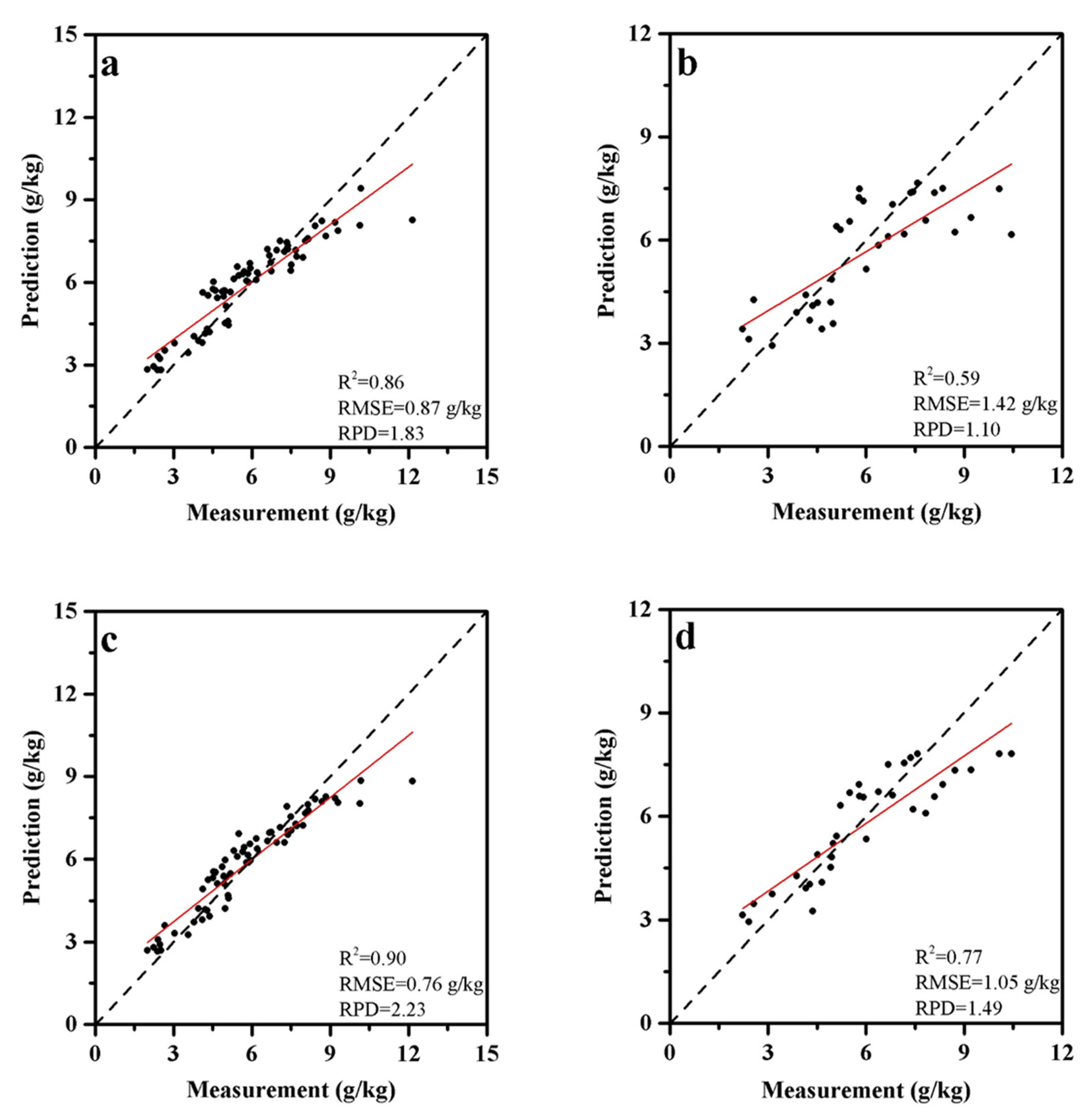
3.4. The Results of Different SOC Predictors on RF Models

The prediction results of the RF models with different predictors are shown in Table 6 and Figure 3. In the calibration set of the SOC prediction model, R2 = 0.86, RMSE = 0.87 g/kg and RPD = 1.83. In the validation set, R2 = 0.59, RMSE = 1.42 g/kg, RPD = 1.10. After adding the sensitive terrain factors (elevation, MaxC, MinC), the R2 of the calibration set’s optimal SOC prediction model was 0.90; the RMSE was 0.76 g/kg; the RPD was 2.23, while in the validation set, R2 = 0.77, RMSE = 1.05 g/kg and RPD = 1.49. The stability, accuracy and prediction ability of the RF model with sensitive terrain factors were higher than those of the original band modeling.

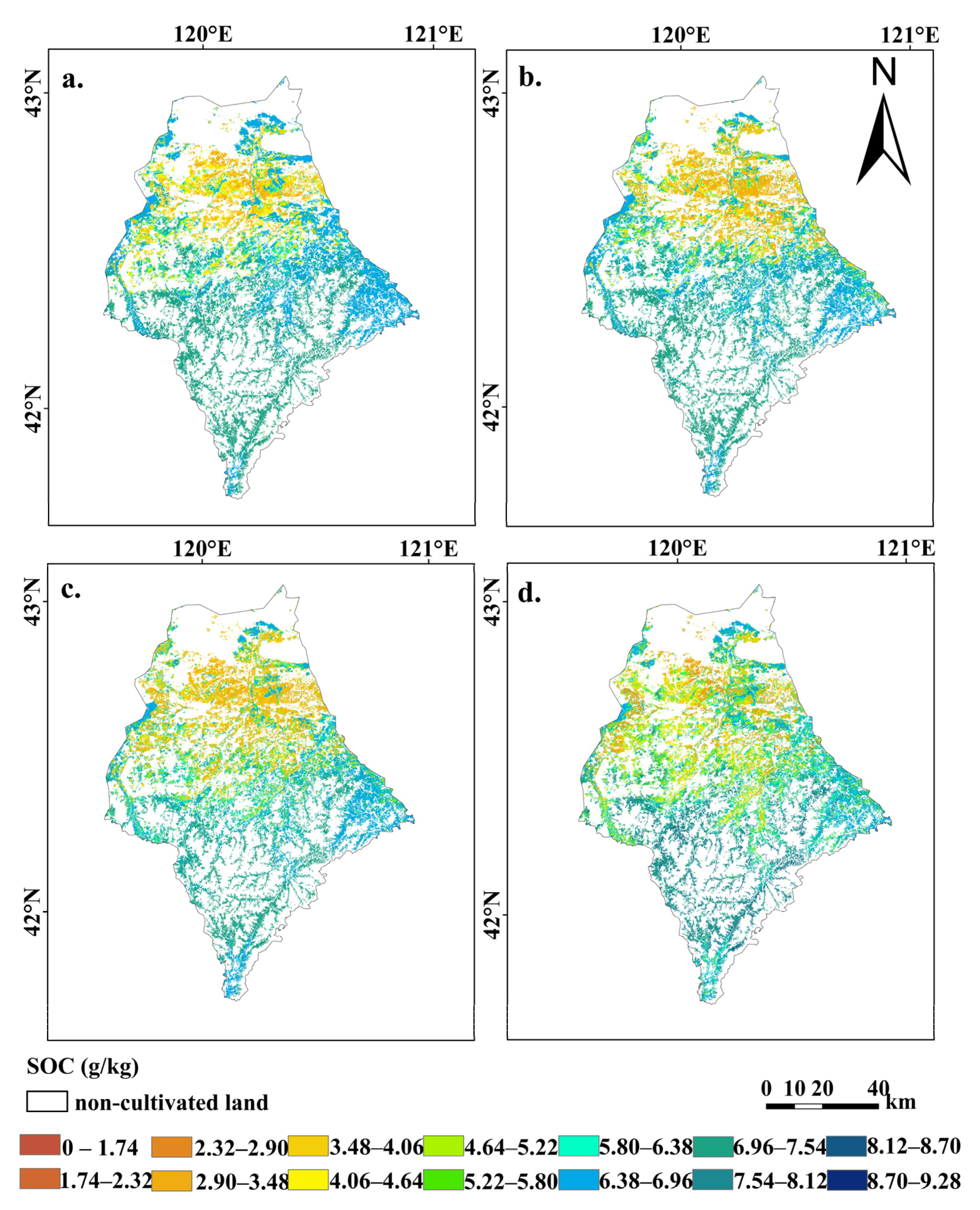
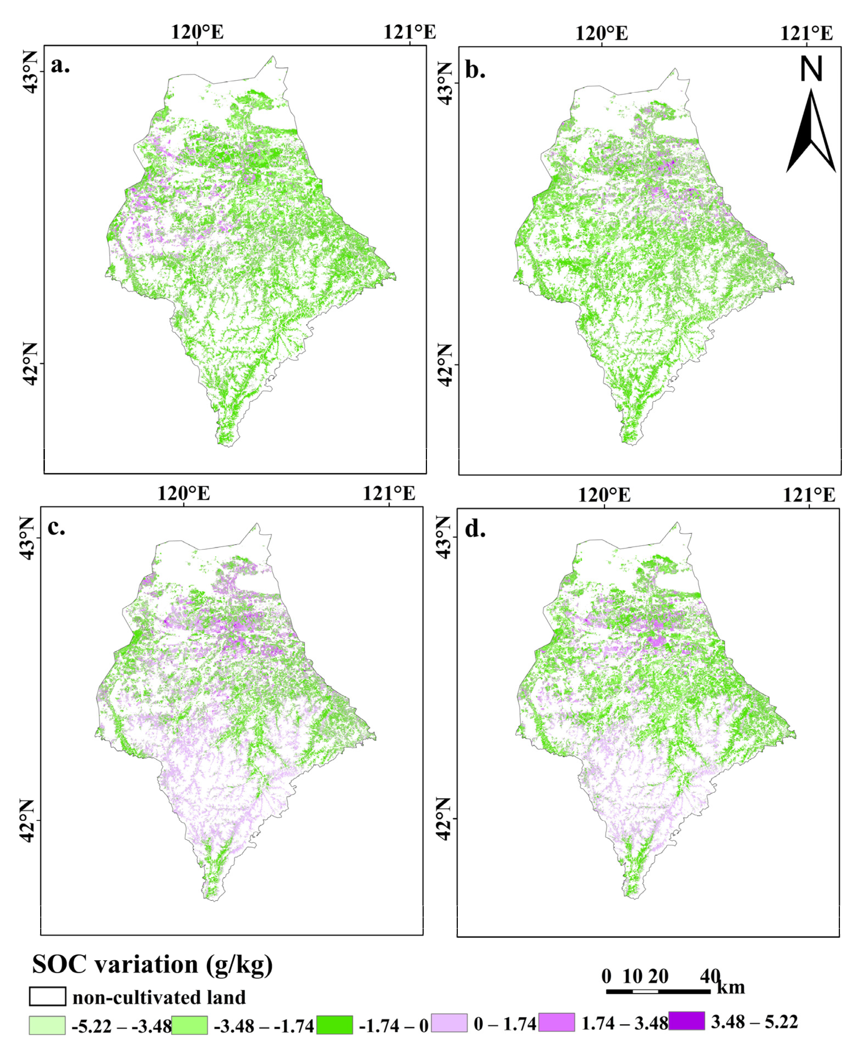
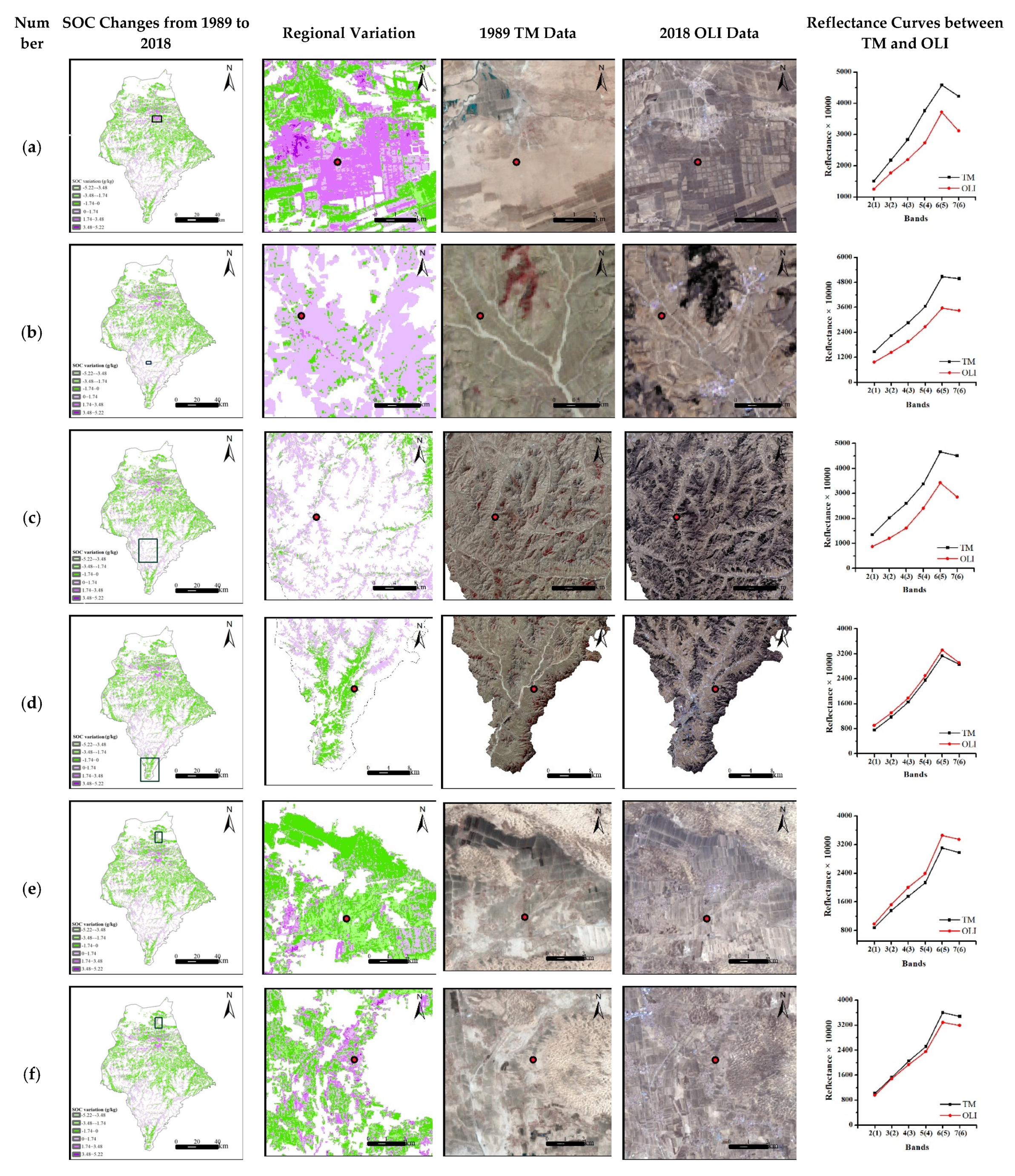
3.5. Spatiotemporal Changes in SOC in Aohan Banner from 1989 to 2018

The sensitive bands (red, NIR, SWIR1, SWIR2) and the sensitive terrain factors (elevation, MaxC, MinC) were selected as predictors. Then, we used the RF model for SOC spatiotemporal prediction in 1989, 2001, 2009 and 2018. As shown in Figure 4, the SOC content in Aohan Banner ranged from 0 to 9.28 g/kg, and the SOC was high in the south and low in the north. Specifically, the high-value area was distributed in the high-elevation area in the south, and the low-value area was distributed in the aeolian sandy area in the north. However, from the spatial distribution map of the four periods, we can see that the spatial distribution of SOC changed slightly, while the area of SOC that less than 5.80 g/kg gradually increased (1227.35 km2 in 1989, 1449.11 km2 in 2001, 1782.860 km2 in 2009, 1790.27 km2 in 2018) and had a southward trend of extension.
From 1989 to 2001, the SOC decreased except in the northwestern part of the study area (Figure 5). After 2001, the SOC content in the northern regions increased gradually, but the SOC content was still low. From 2009 to 2018, parts of the SOC in the study area maintained an increasing trend, indicating that afforestation policy, windbreak and sand fixation policy had positive effects. However, the SOC content in the southernmost part decreased throughout the observation period.
In general, the regions with positive SOC growth from 1989 to 2018 were mainly distributed in the south-central regions and parts of the north-central regions, while the regions with negative SOC growth were mainly distributed in the central, southernmost and part of the northern regions. According to the statistics, the area with positive SOC growth was 1882.77 km2, accounting for 44.08% of the total cultivated land area of Aohan Banner, and the area with negative SOC growth was 2388.76 km2, accounting for 55.92% of the total cultivated land area of Aohan Banner. The SOC in Aohan Banner has changed dynamically in the past 30 years, and the area with negative growth was larger than that with positive growth. As a result, the overall trend was that of degradation.

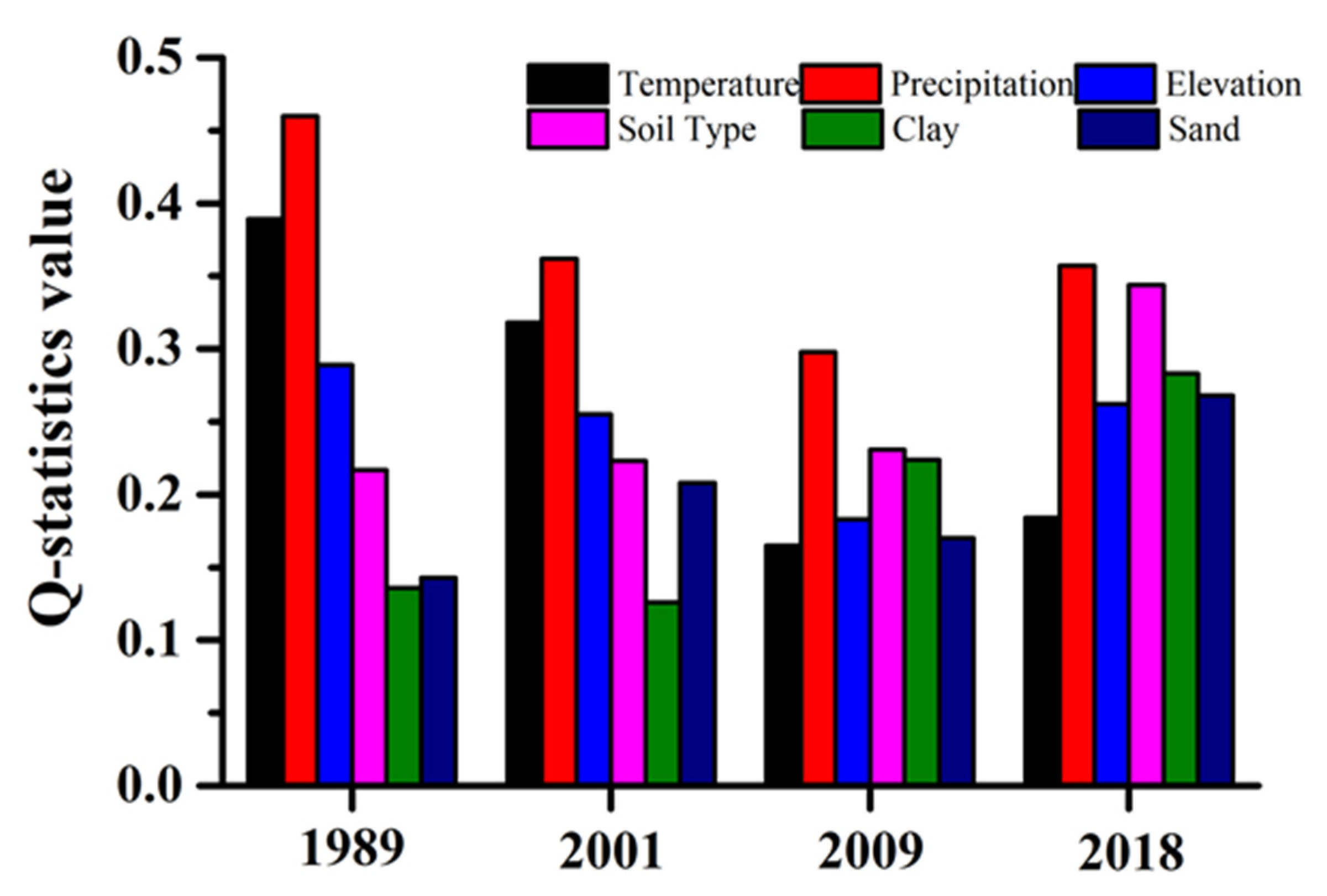
3.6. Driving Factors of Spatiotemporal Changes in Soil Organic Carbon (SOC)

Our results showed that climate change (temperature, precipitation), terrain attributes (elevation), soil types and soil texture (clay, sandy soil) had joint impacts on the spatial distribution of SOC (p < 0.01), while climate change (temperature, precipitation) and human activities (carbon input, GDP) caused temporal differences in SOC (p < 0.01).
As shown in Figure 6, the Q-statistic values of precipitation in 1989, 2001, 2009 and 2018 were larger than those of other factors, which played a leading role in the spatial change in Aohan Banner. However, there is no uniform law of the influence of the other five factors on SOC. Regarding the temporal variation in 1989–2018 (Figure 7), the Q-statistic values on the change of precipitation, temperature, carbon input and GDP increased gradually. Compared with temperature (q = 0.09) and precipitation (q = 0.10), the carbon input (q = 0.14) and GDP (q = 0.15) explained more of the SOC temporal variation. Some man-made measures, such as tillage measures, straw returning and ecological protection projects, led to carbon input change, thus, making carbon input an important factor influencing SOC change, while urban expansion leads to frequent human interference, which is an important embodiment of economic growth, making SOC reduction.

4. Discussions

4.1. The Performance of Different Variables in SOC Mapping

Landsat can realize the analysis of time-series. However, there were some differences in the spectral characteristics obtained by the TM and OLI sensors used in this paper. Due to the intersection of the TM, ETM + and OLI sensors [28,29,30], ETM+ was used as a link to correct the three sensors, and this method increased the accuracy of the Landsat time-series data.
In our study, the Red, NIR, SWIR1 and SWIR2 indices were selected as the variables in the RF models due to the high correlation with SOC, with an R2 of 0.59. Band reflectance information also applied to the SOC prediction in other regions. Dou et al. [37] and Jin et al. [38] used the optimal band combination calculated from MODIS and Landsat to predict SOC in the Songnen Plain and Sanjiang Plain, respectively, with R2 ranging from 0.405 to 0.701. However, the field conditions are complex; even in the bare soil window period, the SOC content can be affected by the environment, soil straw and other factors. Therefore, it is difficult to estimate the spatial distribution of SOC accurately only by band reflectance, especially in the agro-pastoral ecotone with low SOC content.
There is a strong relationship between the topography and the quantity and quality of SOC accumulation [13]. The study area with higher elevation is mainly a mountainous forest vegetation belt with rich vegetation types, water conservation, biomass accumulation and a limited decomposition rate, which is conducive to SOC accumulation; thus, SOC showed an increasing trend [39]. The terrain of the study area changes at elevations of 303–1257 m and is plain in the north and hilly in the south. According to the obvious terrain difference in Aohan Banner, elevation can be used as auxiliary information to improve the accuracy and stability of the SOC prediction model. The size of the terrain curvature value reflects the deformation degree, and the positive-negative curvature values reflect the concave-convex terrain. The distribution and change in terrain curvature can measure the degree of terrain deformation. The larger the absolute value of the curvature is, the more frequent the change is, and the easier it is to enrich, store and flow SOC. Profile curvature and plane curvature are related to soil erosion and deposition. Compared with the surrounding areas, profile curvature and plane curvature have smaller degrees of land deformation on a relatively gentle slope, which is conducive to SOC accumulation [13]. The reason is that the gentle terrain curvature is always accompanied by a smaller slope in the basin and is located at the foot of the slope, where soil nutrients are higher, and SOC is enriched. Moreover, the aboveground vegetation grew well, so the SOC density was higher. In addition, the profile curvature mainly affects the soil water content, and the concave hillside and convergent hillside have higher soil water contents. At a certain temperature, the metabolism of plants in high soil water content areas is accelerated, and the carbon sequestration capacity is strengthened, which can effectively prevent soil erosion. However, the area within the 0–3° slope is mostly characterized by eolian soils with sandy textures and poor structure, and the slope did not play a leading role in SOC. When the slope was greater than 3°, with the increase in slope, soil erosion intensified; soil fertility declined; SOC accumulation decreased. Furthermore, in the long term, water erosion is associated with the loss of nutrients from the soil towards the lower parts of the slopes (Figure A1). MaxC and MinC contain all the surface information, and SOC is more sensitive to MaxC and MinC; thus, MaxC and MinC can be used as auxiliary information to improve the accuracy and stability of the SOC prediction model.

4.2. The Drivers of SOC Spatiotemporal Changes

Precipitation was the most important factor that affected the spatial distribution of SOC [40], and it affected SOC together with temperature, elevation, soil type and texture (p < 0.01). Sufficient precipitation can promote microbial metabolism and increase soil carbon emissions [41]. Precipitation is more important than temperature to the temporal change in SOC (Figure 6). The higher the temperature is, the faster the decomposition rate of SOC is, and the lower the retention of SOC is. Climate warming will increase soil microbial enzyme activity, and then soil heterotrophic respiration will increase [41,42]. Parent materials are one of the main factors of soil formation. The mineral composition of parent materials determines the texture component of the soil and forms different soil types. The difference in soil types leads to different SOC contents. In the study area, high SOC contents are always accompanied by high clay and silt contents, and the texture is relatively loose, while low SOC contents usually have high sand contents [43]. In the soil types of Aohan Banner, cinnamon soils have a higher clay content. Clay mainly affects the formation of aggregates, protects SOC from decomposition and makes the water retention capacity of cinnamon soils larger; these factors are all conducive to SOC aggregation. The sand content of aeolian soils was the highest, reaching 77.25% (Table A1), and the water retention capacity was the worst, with the SOC content being the lowest. Aeolian soils in Aohan Banner were mainly distributed in the northern desert area. The young soil that developed on semi-fixed and fixed dunes is mainly sandy soil with low fertility, more or less covered by psammophilous vegetation. The content of SOC was 4.52 g/kg, lower than that of other areas in Aohan Banner. The gray fluvo-aquic soil was mainly distributed along the riverbank within the low river valley area, where the groundwater level was high; the surface salinity was present; the content of SOC was low, with a value of 5.51 g/kg. Castanozeras soil was mainly distributed in the middle and north of the study area, which is 300–600 m above sea level. The low content of SOC was mainly due to the lack of water. The impact of elevation on SOC is described in Section 4.1.
Anthropogenic activities (carbon input, GDP) had a larger impact on SOC temporal change than did climate factors (temperature and precipitation) (Figure 7). SOC accumulation was large because the SOC input from aboveground and underground plants was greater than the decomposition of SOC [20]. Many studies have shown that carbon input and decomposition caused by man-made measures, such as tillage measures, straw returning and ecological protection projects, have an important impact on SOC change [44,45]. In Aohan Banner, after the dry land was transferred into the paddy field (Figure 8a), the soil moisture increased greatly. Soil moisture was closely related to the structure, function, enzyme activity of the soil microbial community and the change in the fungal community, which limited their contributions to SOC decomposition [30].
After the long-term implementation of the terracing slope cropland project (Figure 8b), the effect of sediment and runoff reduction will be significantly enhanced. Additionally, the carbon input (q = 0.14) from plants has an important relationship with the temporal change in SOC in Aohan Banner. The 3-North Shelter Forest Program has been implemented since 1979 [46]. Until 2009, Aohan Banner had a forest area of 5,290,000 mu, accounting for 42.5% of the total land area, which was four times that in 1978 and became the “first county of afforestation in China”. The increase in forest area (Figure 8c) led to an increase in forest carbon reserves, which led to an increase in the carbon reserves of the whole ecosystem, for more humus will be formed on the surface of forest land, and more SOC will be accumulated in cultivated land as rainwater washes into the stream valleys. The fourth phase of the 3-North Shelter Forest Program (2001–2010) focused on the prevention and control of desertification. In the agro-pastoral ecotone of northern China, the SOC that increased from sandy land to woodland was close to 1.74 kg m−2, and the SOC that increased from sandy land to cultivated land was approximately 0.58 kg m−2 [35]. In addition, the Beijing Tianjin sandstorm source project [47], CDM carbon sink project [48] and other sandstorm control measures have had positive effects on the improvement of SOC in the northern desert area (Figure 8f). Due to the implementation of the straw returning policy, the carbon input from crop roots in Aohan Banner showed an overall upward trend from 1989 to 2018 (Figure 9). The above measures led to an increase in SOC in 1989–2018. However, the burning of plastic film and some straw consumes a large amount of organic matter, resulting in soil carbon losses, and the increase in SOC has not been high enough to compensate for the loss of SOC. Besides, urban construction land expansion is an important embodiment of economic growth. The expansion of urban construction land (Figure 8d) occupies a large amount of cultivated land, and human activities are more intensive. Rapid urbanization is an important factor that causes SOC reductions. The frequent interference and demand for anthrogenic activities have imposed pressure on the use of agricultural water. Moreover, typical urban land development practices have destroyed soil aggregates. The proportion of aggregates has been reduced and has caused carbon loss associated with aggregates in the topsoil [49]. Rapid urban expansion leads to soil carbon loss; thus, agriculture transforms soil from fertile soil to marginal soil [50]. In addition, due to the vulnerability of the sandy ecosystem (Figure 8e), although sandy land consolidation measures played a positive role in relation to SOC after 2009, negative human activities (poor management measures and grazing) promoted the gradual development of fixed and semifixed dunes, and plants were replaced by dunes. Additionally, large-scale cultivated land destroyed the compression resilience of the soil surface, causing the content of SOC to decrease to a certain extent from 1989 to 2018.

5. Conclusions

Our results consider the reflectance of sensitive bands and terrain factors as the inputs of the SOC prediction model. The addition of terrain factors into the RF model achieved the greater precision of SOC spatiotemporal mapping in the agro-pastoral ecotone. However, another predictor such as parent material should be taken into further study, as it affects the physical and chemical properties and mineral composition of soil.
This paper revealed that SOC in the cultivated land of Aohan Banner showed a dynamic change from 1989 to 2018, with a general trend of degradation. Precipitation was the main controlling factor of the spatial change in SOC in Aohan Banner, and it affected the spatial change in SOC in combination with temperature, elevation, soil type, clay and silt. Anthropogenic activities (carbon input and GDP) had a greater impact on the SOC temporal variation than did climate factors (temperature and precipitation), making human activities the dominant factor affecting SOC temporal variation in Aohan Banner. The reduction in SOC in the Aohan Banner was mainly due to urban expansion and dune movement, and the main reason for the SOC increase was the implementation of large-scale ecological restoration projects and agricultural cultivation measures (dry land to paddy field, slope to terrace). In this paper, the SOC of Aohan Banner in the last 30 years was predicted using RS, GIS, the RF model and the GDM; thus, its spatiotemporal distribution and driving factors were comprehensively analyzed. The results of this paper increase our understanding of the spatiotemporal changes in SOC in the agro-pastoral ecotone. The typical agro-pastoral ecotone shows a certain degradation state, and it is necessary to strengthen protection measures. Reasonable and effective man-made management measures play important roles in the accumulation of SOC and help to provide suggestions for sustainable soil management in the agro-pastoral ecotone in the future.

Author Contributions

Conceptualization, L.W., H.L. (Huanjun Liu) and S.Z.; methodology, L.W., X.W. and X.M.; software, L.W. and X.W.; validation, H.L. (Huanjun Liu), X.W., X.M., C.L., H.L. (Houxuan Li), L.M. and Y.W.; formal analysis, L.W.; investigation, L.W.; resources, H.L. (Huanjun Liu); data curation, L.W.; writing—original draft preparation, L.W.; writing—review and editing, L.W. and X.W.; visualization, X.W., D.W., B.Q.; supervision, S.Z., D.W., B.Q.; project administration, H.L. (Huanjun Liu); funding acquisition, H.L (Huanjun Liu). All authors have read and agreed to the published version of the manuscript.

Funding

This research was funded by the National Natural Science Foundation of China (41671438) and Department of Science and Technology of Jilin Province (20170301001NY).

Data Availability Statement

No new data were created or analyzed in this study. Data sharing is not applicable to this article.

Conflicts of Interest

The authors declare no conflict of interest.

Appendix A

Figure A1. The relationship of slope and soil organic carbon (SOC).
Remotesensing 13 03607 g0a1
Table A1. The mean value of soil organic carbon (SOC) and soil texture in different soil types.
Soil TypeSOC (g/kg)Silt (%)Sand (%)Clay (%)
gray fluvo–aquic soil5.5129.0050.9320.07
cinnamon soil7.5631.3046.9722.73
Castanozeras soil5.2230.1452.2817.58
Aeolian soils4.5214.5077.258.25

References

  1. Post, W.M.; Emanuel, W.R.; Zinke, P.J.; Stangenberger, A.G. Soil Carbon Pools And World Life Zones. Nature 1982, 298, 156–159. [Google Scholar] [CrossRef]
  2. Wang, J.; He, T.; Lv, C.; Chen, Y.; Jian, W. Mapping soil organic matter based on land degradation spectral response units using Hyperion images. Int. J. Appl. Earth Obs. 2010, 12, S171–S180. [Google Scholar] [CrossRef]
  3. Wood, S.A.; Baudron, F. Soil organic matter underlies crop nutritional quality and productivity in smallholder agriculture. Agric. Ecosyst. Environ. 2018, 266, 100–108. [Google Scholar] [CrossRef]
  4. Meng, X.; Bao, Y.; Liu, J.; Liu, H.; Zhang, X.; Zhang, Y.; Wang, P.; Tang, H.; Kong, F. Regional soil organic carbon prediction model based on a discrete wavelet analysis of hyperspectral satellite data. Int. J. Appl. Earth Obs. 2020, 89, 102111. [Google Scholar] [CrossRef]
  5. Seema; Ghosh, A.K.; Das, B.S.; Reddy, N. Application of VIS-NIR spectroscopy for estimation of soil organic carbon using different spectral preprocessing techniques and multivariate methods in the middle Indo-Gangetic plains of India. Geoderma Reg. 2020, 23, e00349. [Google Scholar] [CrossRef]
  6. Zhang, Z.; Ding, J.; Zhu, C.; Wang, J.; Ma, G.; Ge, X.; Li, Z.; Han, L. Strategies for the efficient estimation of soil organic matter in salt-affected soils through Vis-NIR spectroscopy: Optimal band combination algorithm and spectral degradation. Geoderma 2021, 382, 114729. [Google Scholar] [CrossRef]
  7. Padilha, M.C.D.C.; Vicente, L.E.; Dematte, J.A.M.; Loebmann, D.G.D.S.W.; Vicente, A.K.; Salazar, D.F.U.; Guimaraes, C.C.B. Using Landsat and soil clay content to map soil organic carbon of oxisols and Ultisols near Sao Paulo, Brazil. Geoderma Reg. 2020, 21, e00253. [Google Scholar] [CrossRef]
  8. Ingleby, H.R.; Crowe, T.G. Reflectance models for predicting organic carbon in Saskatchewan soils. Can. Agric. Eng. 2000, 42, 57–63. [Google Scholar]
  9. Grinand, C.; Le Maire, G.; Vieilledent, G.; Razakarnanarivo, H.; Razafimbelo, T.; Bernoux, M. Estimating temporal changes in soil carbon stocks at ecoregional scale in Madagascar using remote-sensing. Int. J. Appl. Earth Obs. 2017, 54, 1–14. [Google Scholar] [CrossRef]
  10. Chen, D.; Chang, N.; Xiao, J.; Zhou, Q.; Wu, W. Mapping dynamics of soil organic matter in croplands with MODIS data and machine learning algorithms. Sci. Total Environ. 2019, 669, 844–855. [Google Scholar] [CrossRef] [PubMed]
  11. Yang, Q.Y.; Jiang, Z.C.; Li, W.J.; Li, H. Prediction of soil organic matter in peak-cluster depression region using kriging and terrain indices. Soil Tillage Res. 2014, 144, 126–132. [Google Scholar] [CrossRef]
  12. Zhang, S.; Huang, Y.; Shen, C.; Ye, H.; Du, Y. Spatial prediction of soil organic matter using terrain indices and categorical variables as auxiliary information. Geoderma 2012, 171, 35–43. [Google Scholar] [CrossRef]
  13. Grimm, R.; Behrens, T.; Marker, M.; Elsenbeer, H. Soil organic carbon concentrations and stocks on Barro Colorado Island—digital soil mapping using Random Forests analysis. Geoderma 2008, 146, 102–113. [Google Scholar] [CrossRef]
  14. Zeraatpisheh, M.; Ayoubi, S.; Jafari, A.; Tajik, S.; Finke, P. Digital mapping of soil properties using multiple machine learning in a semi-arid region, central Iran. Geoderma 2019, 338, 445–452. [Google Scholar] [CrossRef]
  15. Fissore, C.; Dalzell, B.J.; Berhe, A.A.; Voegtle, M.A.; Evans, M.A.; Wu, A. Influence of topography on soil organic carbon dynamics in a Southern California grassland. Catena 2017, 149, 140–149. [Google Scholar] [CrossRef]
  16. Cai, A.; Feng, W.; Zhang, W.; Xu, M. Climate, soil texture, and soil types affect the contributions of fine-fraction-stabilized carbon to total soil organic carbon in different land uses across China. J. Environ. Manag. 2016, 172, 2–9. [Google Scholar] [CrossRef]
  17. Chen, Q.; Niu, B.; Hu, Y.; Luo, T.; Zhang, G. Warming and increased precipitation indirectly affect the composition and turnover of labile-fraction soil organic matter by directly affecting vegetation and microorganisms. Sci. Total Environ. 2020, 714, 136787. [Google Scholar] [CrossRef]
  18. Chen, L.; Jing, X.; Flynn, D.F.B.; Shi, Y.; Kuehn, P.; Scholten, T.; He, J.-S. Changes of carbon stocks in alpine grassland soils from 2002 to 2011 on the Tibetan Plateau and their climatic causes. Geoderma 2017, 288, 166–174. [Google Scholar] [CrossRef]
  19. Bahadori, M.; Chen, C.; Lewis, S.; Boyd, S.; Rashti, M.R.; Esfandbod, M.; Garzon-Garcia, A.; Van Zwieten, L.; Kuzyakov, Y. Soil organic matter formation is controlled by the chemistry and bioavailability of organic carbon inputs across different land uses. Sci. Total Environ. 2021, 770, 145307. [Google Scholar] [CrossRef]
  20. Xie, E.; Zhang, Y.; Huang, B.; Zhao, Y.; Shi, X.; Hu, W.; Qu, M. Spatiotemporal variations in soil organic carbon and their drivers in southeastern China during 1981–2011. Soil Tillage Res. 2021, 205, 104763. [Google Scholar] [CrossRef]
  21. Zhao, Y.; Wang, M.; Hu, S.; Zhang, X.; Ouyang, Z.; Zhang, G.; Huang, B.; Zhao, S.; Wu, J.; Xie, D.; et al. Economics- and policy-driven organic carbon input enhancement dominates soil organic carbon accumulation in Chinese croplands. Proc. Natl. Acad. Sci. USA 2018, 115, 4045–4050. [Google Scholar] [CrossRef] [PubMed] [Green Version]
  22. Du, X.; Zhang, L.-F. Succession and Enhancement Mechanism of Ecosystem Productivity in the De-farming Area of the Ecotone Between Agriculture and Animal Husbandry in North China. Agric. Sci. China 2008, 7, 487–496. [Google Scholar] [CrossRef]
  23. Yao, Y.; Ge, N.; Wei, X.; Fu, W.; Shao, M.; Zhao, X.; Ingwersen, J. Responses of soil organic carbon mineralization and its temperature sensitivity to re-vegetation in the agro-pastoral ecotone of northern China. Eur. J. Soil Biol. 2021, 103, 103278. [Google Scholar] [CrossRef]
  24. Wang, X.; Li, Y.; Gong, X.; Niu, Y.; Liu, J. Changes of soil organic carbon stocks from the 1980s to 2018 in northern China’s agro-pastoral ecotone. Catena 2020, 194, 104722. [Google Scholar] [CrossRef]
  25. O’Kelly, B.C. Accurate determination of moisture content of organic soils using the oven drying method. Dry. Technol. 2004, 22, 1767–1776. [Google Scholar] [CrossRef]
  26. Nelson, D.W.; Sommers, L.E. Total carbon, organic carbon, and organic matter. In Methods of Soil Analysis, 3rd ed.; Sparks, D.L., Ed.; SSSA and ASA: Madison, WI, USA, 1996; pp. 961–1010. [Google Scholar]
  27. Shi, X.Z.; Yu, D.S.; Xu, S.X.; Warner, E.D.; Wang, H.J.; Sun, W.X.; Zhao, Y.C.; Gong, Z.T. Cross-reference for relating Genetic Soil Classification of China with WRB at different scales. Geoderma 2010, 155, 344–350. [Google Scholar] [CrossRef]
  28. Meng, L.; Zhang, X.L.; Liu, H.; Guo, D.; Yan, Y.; Qin, L.; Pan, Y. Estimation of Cotton Yield Using the Reconstructed Time-Series Vegetation Index of Landsat Data. Can. J. Remote Sens. 2017, 43, 244–255. [Google Scholar] [CrossRef]
  29. Mishra, N.; Helder, D.; Barsi, J.; Markham, B. Continuous calibration improvement in solar reflective bands: Landsat 5 through Landsat 8. Remote Sens. Environ. 2016, 185, 7–15. [Google Scholar] [CrossRef] [Green Version]
  30. Pu, X.; Cheng, H.; Tysklind, M.; Xie, J.; Lu, L.; Yang, S. Indications of soil properties on dissolved organic carbon variability following a successive land use conversion. Ecol. Eng. 2018, 117, 115–119. [Google Scholar] [CrossRef]
  31. Pouladi, N.; Møller, A.B.; Tabatabai, S.; Greve, M.H. Mapping soil organic matter contents at field level with Cubist, Random Forest and kriging. Geoderma 2019, 342, 85–92. [Google Scholar] [CrossRef]
  32. Teng, H.; Rossel, R.A.V.; Shi, Z.; Behrens, T. Updating a national soil classification with spectroscopic predictions and digital soil mapping. Catena 2018, 164, 125–134. [Google Scholar] [CrossRef]
  33. Luo, L.; Mei, K.; Qu, L.; Zhang, C.; Chen, H.; Wang, S.; Di, D.; Huang, H.; Wang, Z.; Xia, F.; et al. Assessment of the Geographical Detector Method for investigating heavy metal source apportionment in an urban watershed of Eastern China. Sci. Total Environ. 2019, 653, 714–722. [Google Scholar] [CrossRef] [PubMed] [Green Version]
  34. Qiao, P.; Yang, S.; Lei, M.; Chen, T.; Dong, N. Quantitative analysis of the factors influencing spatial distribution of soil heavy metals based on geographical detector. Sci. Total Environ. 2019, 664, 392–413. [Google Scholar] [CrossRef] [PubMed]
  35. Wang, X.; Li, Y.; Gong, X.; Niu, Y.; Chen, Y.; Shi, X.; Li, W. Storage, pattern and driving factors of soil organic carbon in an ecologically fragile zone of nothern China. Geoderma 2019, 343, 155–165. [Google Scholar] [CrossRef]
  36. Lewis-Beck, M.S.; Tien, C. Election Forecasting for Turbulent Times. PS-Poli. Sci. Pol. 2012, 45, 625–629. [Google Scholar] [CrossRef]
  37. Dou, X.; Wang, X.; Liu, H.; Zhang, X.; Meng, L.; Pan, Y.; Yu, Z.; Cui, Y. Prediction of soil organic matter using multi-temporal satellite images in the Songnen Plain, China. Geoderma 2019, 356, 113896. [Google Scholar] [CrossRef]
  38. Jin, X.; Song, K.; Du, J.; Liu, H.; Wen, Z. Comparison of different satellite bands and vegetation indices for estimation of soil organic matter based on simulated spectral configuration. Agric. Forest Meteorol. 2017, 244–245, 57–71. [Google Scholar] [CrossRef]
  39. Teng, M.; Zeng, L.; Xiao, W.; Huang, Z.; Zhou, Z.; Yan, Z.; Wang, P. Spatial variability of soil organic carbon in Three Gorges Reservoir area, China. Sci. Total Environ. 2017, 599, 1308–1316. [Google Scholar] [CrossRef]
  40. Wang, D.D.; Shi, X.Z.; Wang, H.J.; Weindorf, D.C.; Yu, D.S.; Sun, W.X.; Ren, H.Y.; Zhao, Y.C. Scale Effect of Climate and Soil Texture on Soil Organic Carbon in the Uplands of Northeast China. Pedosphere 2010, 20, 525–535. [Google Scholar] [CrossRef]
  41. Zhao, C.; Miao, Y.; Yu, C.; Zhu, L.; Wang, F.; Jiang, L.; Hui, D.; Wan, S. Soil microbial community composition and respiration along an experimental precipitation gradient in a semiarid steppe. Sci. Rep. 2016, 6, 24317. [Google Scholar] [CrossRef] [Green Version]
  42. Lybrand, R.A.; Rasmussen, C. Quantifying Climate and Landscape Position Controls on Soil Development in Semiarid Ecosystems. Soil. Sci. Soc. Am. J. 2015, 79, 104–116. [Google Scholar] [CrossRef] [Green Version]
  43. Melero, S.; Ruiz Porras, J.C.; Francisco Herencia, J.; Madejon, E. Chemical and biochemical properties in a silty loam soil under conventional and organic management. Soil Tillage Res. 2006, 90, 162–170. [Google Scholar] [CrossRef]
  44. Huang, B.; Sun, W.; Zhao, Y.; Zhu, J.; Yang, R.; Zou, Z.; Ding, F.; Su, J. Temporal and spatial variability of soil organic matter and total nitrogen in an agricultural ecosystem as affected by farming practices. Geoderma 2007, 139, 336–345. [Google Scholar] [CrossRef]
  45. Shi, S.Q.; Cao, Q.W.; Yao, Y.M.; Tang, H.J.; Yang, P.; Wu, W.B.; Xu, H.Z.; Liu, J.; Li, Z.G. Influence of Climate and Socio-Economic Factors on the Spatio-Temporal Variability of Soil Organic Matter: A Case Study of Central Heilongjiang Province, China. J. Integr. Agric. 2014, 13, 1486–1500. [Google Scholar] [CrossRef]
  46. Wang, X.M.; Zhang, C.X.; Hasi, E.; Dong, Z.B. Has the Three Norths Forest Shelterbelt Program solved the desertification and dust storm problems in arid and semiarid China? J. Arid. Environ. 2010, 74, 13–22. [Google Scholar] [CrossRef]
  47. Wang, S.; Zhang, B.; Wang, S.; Xie, G.D. Dynamic changes in water conservation in the Beijing Tianjin Sandstorm Source Control Project Area: A case study of Xilin Gol League in China. J. Clean. Prod. 2021, 293, 126054. [Google Scholar] [CrossRef]
  48. Lo, A.Y.; Cong, R. After CDM: Domestic carbon offsetting in China. J. Clean. Prod. 2017, 141, 1391–1399. [Google Scholar] [CrossRef] [Green Version]
  49. Chen, Y.; Day, S.D.; Wick, A.F.; McGuire, K.J. Influence of urban land development and subsequent soil rehabilitation on soil aggregates, carbon, and hydraulic conductivity. Sci. Total Environ. 2014, 494, 329–336. [Google Scholar] [CrossRef] [PubMed]
  50. Abd-Elmabod, S.K.; Fitch, A.C.; Zhang, Z.; Ali, R.R.; Jones, L. Rapid urbanisation threatens fertile agricultural land and soil carbon in the Nile delta. J. Environ. Manag. 2019, 252, 109668. [Google Scholar] [CrossRef]
Figure 1. (a) Locations of the agro-pastoral ecotone of northern China and their relationships with the land-use and cover types in 2015. (b) Locations of the sampling sites with a relative elevation map in the study area.
Remotesensing 13 03607 g001
Figure 2. (a). Reflectance characteristics of different SOC values of OLI. (b). Comparison of spectral characteristics between OLI and TM.
Remotesensing 13 03607 g002
Figure 3. Relationships between measured and estimated soil carbon (SOC) values. (a,b) are the calibration dataset and validation dataset using the red, NIR, SWIR1 and SWIR2 bands. (c,d) are the calibration dataset and validation dataset using the inputs of red, NIR, SWIR1, SWIR2 and elevation, MaxC and MinC.
Remotesensing 13 03607 g003
Figure 4. Spatial distributions of the soil organic carbon (SOC) in 1989 (a), 2001 (b), 2009 (c) and 2018 (d) with a resolution of 30 m.
Remotesensing 13 03607 g004
Figure 5. Spatial pattern of the changes in soil organic carbon (SOC) during the periods of 1989–2001 (a), 2001–2009 (b), 2009–2018 (c) and 1989–2018 (d).
Remotesensing 13 03607 g005
Figure 6. Q-statistic values in the geodetector analysis of the predictor importance for soil organic matter (SOC) in Aohan Banner. (All variables in Figure 5 show strongly significant effects at p < 0.01).
Remotesensing 13 03607 g006
Figure 7. The impact of anthropogenic activities on the changes in soil organic carbon (SOC) in Aohan Banner.
Remotesensing 13 03607 g007
Figure 8. A comparison of the remote sensing data between 1989 and 2018 in typical areas (af) (From left to right are Scheme 1989. to 2018, regional variation, 1989 TM data, 2018 OLI data and reflectance curves between TM and OLI in the places of the dots, respectively).
Remotesensing 13 03607 g008
Figure 9. Crop root carbon inputs since 1989 (carbon inputs by roots were estimated using the crop yield data referenced by [21]).
Remotesensing 13 03607 g009
Table 1. Landsat image acquisition and date.
ImagesDate
TM25 March 1989
TM26 March 2001
TM1 April 2009
OLI25 March 2018
Table 2. The correction coefficients of ETM+, TM and OLI.
BandsRegression Model
between ETM+ and TM
R2RMSE
(Reflectance)
Regression Model
between OLI and ETM+
R2RMSE
(Reflectance)
RedETM+ =1.071×TM−0.0160.9800.013OLI = 1.010×ETM+ −0.0110.9480.025
NIRETM+ =1.076×TM−0.0230.9790.013OLI = 0.988×ETM+ −0.0150.9430.028
SWIR1ETM+ =1.048×TM−0.0240.9840.022OLI = 0.966×ETM+ −0.0020.9540.035
SWIR2ETM+ =1.037×TM−0.0220.9820.024OLI = 0.911×ETM+ +0.0070.9440.043
Table 3. The auxiliary variables used in the study area.
ParametersPurposeData Sources
ElevationPredictor/Spatial driving factor https://search.asf.alaska.edu/#/, accessed on 25 March 2020
MaxCPredictorExtracted by ENVI 5.3
MinCPredictorExtracted by ENVI 5.3
ClaySpatial driving factorhttps://www.resdc.cn/, accessed on 25 March 2020
Soil TypeSpatial driving factorhttps://www.resdc.cn/, accessed on 25 March 2020
PrecipitationSpatial/temporal driving factorhttps://data.cma.cn/; https://www.resdc.cn/, accessed on 25 March 2020
TemperatureSpatial/temporal driving factorhttps://data.cma.cn/; https://www.resdc.cn/, accessed on 25 March 2020
C inputSpatial/temporal driving factor http://files.ntsg.umt.edu/data/NTSGProducts/MOD17/, accessed on 25 March 2020
GDPSpatial/temporal driving factorhttps://www.resdc.cn/, accessed on 25 March 2020
Note: MaxC represents maximum curvature; MinC represents minimum curvature; C input represents carbon input; GDP represents Gross National Product.
Table 4. Statistical descriptions of the soil organic carbon (SOC) in the whole, calibration and validation datasets.
SetnMax (g/kg)Min (g/kg)Mean (g/kg)SD (g/kg)SkewnessKurtosisCV/%
Whole dataset10212.182.035.902.110.33−0.1335.82
Calibration
dataset
6812.182.035.872.130.380.0736.34
Validation
dataset
3410.442.265.962.110.240.4235.30
Table 5. The linkage between variables and soil organic carbon (SOC).
BandsCoefficientVIFTerrain FactorsCoefficientVIF
Blue−0.48 **1.29Elevation0.48 **1.30
Green−0.50 **1.33MaxC0.48 **1.29
Red−0.53 **1.39MinC−0.48 **1.29
NIR−0.60 **1.57Aspect−0.111.01
SWIR1−0.64 **1.70Slope0.141.02
SWIR2−0.58 **1.52
Note: MaxC represents maximum curvature; MinC represents minimum curvature; VIF represents variance inflation factor; ** represents a significant correlation at the 0.01 level.
Table 6. Prediction results of RF models with different inputs.
InputR2 calRMSE cal/g/kgRPD calR2 valRMSE val/g/kgRPD val
Red, NIR, SWIR1, SWIR20.860.871.830.591.421.10
Red, NIR, SWIR1, SWIR2 + Elevation + MaxC + MinC0.900.762.230.771.051.49
Note: MaxC represents maximum curvature; MinC represents minimum curvature; R2 cal and R2 val represent the R2 of calibration and validation datasets, respectively; RMSE cal and RMSE val represent the RMSE of calibration and validation datasets, respectively; RPD cal and RPD val represent the RPD of calibration and validation datasets, respectively.
Publisher’s Note: MDPI stays neutral with regard to jurisdictional claims in published maps and institutional affiliations.

