New Channel Errors Estimation Method for Multichannel SAR Based on Virtual Calibration Source

Abstract

The multichannel synthetic aperture radar (SAR) system can effectively overcome the fundamental limitation between high-resolution and wide-swath. However, the unavoidable channel errors will result in a mismatch of the reconstruction filter and false targets in pairs. To address this issue, a novel channel errors calibration method is proposed based on the idea of minimizing the mean square error (MMSE) between the signal subspace and the space spanned by the practical steering vectors. The practical steering matrix of each Doppler bin can be constructed according to the Doppler spectrum. Compared with the time-domain correlation method, the proposed method no longer depends on the accuracy of the Doppler centroid estimation. Besides, compared with the orthogonal subspace method, the proposed method has the advantage of robustness under the condition of large samples by using the diagonal loading technique. To evaluate the performance, the results of simulation data and the real data acquired by the GF-3 dual-channel SAR system demonstrate that the proposed method has higher accuracy and more robustness than the conventional methods, especially in the case of low SNRs and high non-uniformity.

1. Introduction

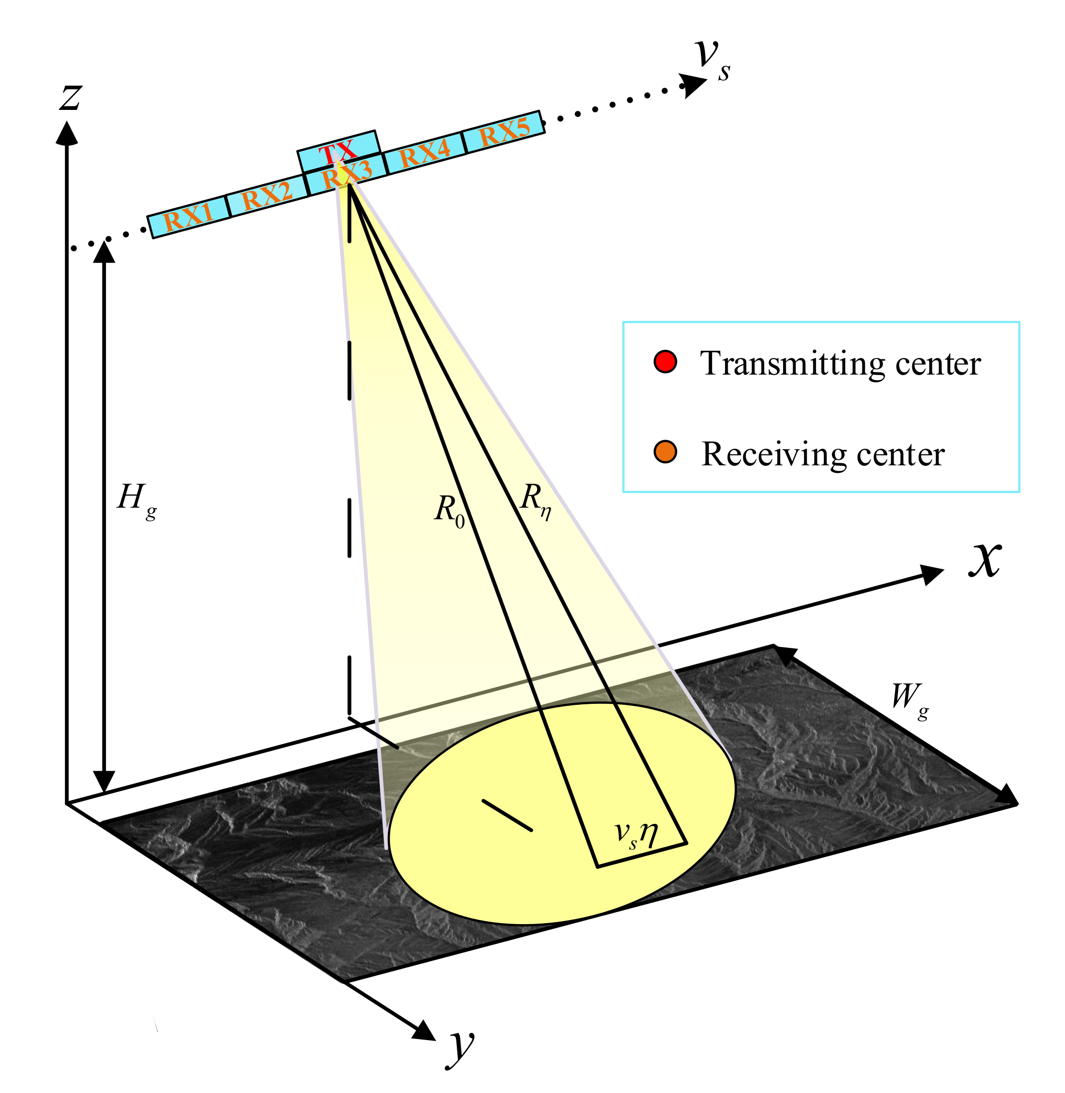
With the development of synthetic aperture radar (SAR) imaging technology, the demand for high-resolution and wide-swath has gradually increased [1,2,3,4,5,6]. For conventional spaceborne SAR systems, it is difficult to achieve high-resolution and wide-swath at the same time. The improvement of the azimuth resolution requires a short antenna in order to obtain a large Doppler bandwidth and a sufficiently high pulse repetition frequency (PRF) to achieve azimuth oversampling, while the wide-swath requires a low PRF in order to avoid range ambiguity [1,2,3]. To effectively overcome these fundamental limitations, in this study, a multichannel SAR system is combined with digital beamforming technology by adding multiple receiving channels in azimuth (see Figure 1). In other words, spatial sampling is used to compensate for the lack of temporal sampling [1,2]. Then, the non-uniformly sampled SAR signal can be suppressed using the digital beamforming (DBF) method [3] or the space-time adaptive processing (STAP) method [4].

However, in practical engineering, errors between the receiving channels are unavoidable. These include the antenna gain, phase, position, and range sampling time delay errors, which will lead to a serious mismatch of the reconstruction filter and result in false targets in pairs. Therefore, it is necessary to accurately calibrate the channel errors in order to improve the performance of ambiguity suppression. During the last few decades, a number of channel calibration methods have been proposed to deal with this problem [5,6,7,8,9,10,11,12,13,14,15,16,17,18,19]. The gain inconsistency error can be calibrated relatively easily by channel balancing [5]. In general, the channel phase error calibration methods can be classified into three categories: the inner calibration [6], time-domain calibration [7,8,9], and range-Doppler domain calibration methods [10,11,12,13,14,15,16,17,18,19].

In [6], Chen et al. proposed an inner calibration method (ICM) based on the gain-phase characteristics of each channel, which estimates phase errors by comparing the gain and phase at the peak value of the signal received by the calibration route. However, the ICM may suffer from performance degradation when the channel mismatch is caused by the antenna because the calibration route bypasses the antenna and directly receives the transmitted signal. To address this issue, the time-domain correlation method (TDCM) was proposed in [7,8,9], which estimates the phase errors as well as the Doppler centroid frequency based on the spatial correlation between adjacent channels. Unfortunately, the estimation of the channel phase errors by the TDCM depends heavily on the accuracy of the Doppler centroid. Meanwhile, with an increase in the number of channels, the average root mean square error of the phase errors increases. To solve these issues, Doppler domain-based calibration methods have been developed on the basis that the spectral components of each Doppler bin can be regarded as virtual signal sources from different known directions. Such methods include subspace-based methods [10,11,12,13,14,15,16,17] and optimal beamforming methods [18,19].

By incorporation with multiple signal classification (MUSIC), Li et al. [10,11,12] proposed the orthogonal subspace method (OSM), which is based on the fact that the signal subspace spanned by the practical steering vectors is orthogonal to the noise subspace. Nevertheless, the performance of the OSM may deteriorate when the number of channels is equal to the ambiguity indexes of the spectrum, because there are not enough degrees of freedom to construct the signal subspace. Meanwhile, in the case of larger samples, the matrices $(\sum {\mathrm{\Gamma }}^H{a}_i^H{U}_N{U}_N^H{a}_i\mathrm{\Gamma })$ of some Doppler bins are close to the singular value, which may lead to inaccurate estimation results. To solve this issue, with reference to direction of arrival (DOA) estimation, Yang et al. [13,14] proposed the signal subspace comparison method (SSCM), which is based on the fact that the space spanned by the signal eigenvectors is equal to that by the practical steering vectors. Thus, the projection matrices of the two subspaces are unique. Unfortunately, in practice, there exists a transition matrix in transformation of basic between the projection spaces, which may degrade the phase error estimation performance of this method. To solve the problem, Zhou et al. [17] proposed a subspace-based method by minimizing the minimum mean square error of the signal subspace. However, the phase error is estimated by the Newton–Raphson method or the optimizer tool, which requires a high computational load. Besides, Zhang et al. [18] proposed a robust phase error calibration method via maximizing the minimum variance distortionless response (MVDR) beamformer output power. However, the performance of the MVDR may be hindered by the fact that the MVDR only maintains the gain of the desired signal constant, neglecting to suppress the unwanted signal. Considering this problem, Huang et al. [19] proposed the orthogonal projection method (OPM), which is based on the idea that the energy of each ambiguity component extracted by the orthogonal projection method is maximized. Unfortunately, the OPM may suffer from a performance degradation because the weight vector of the OPM depends heavily on the array geometry of the SAR system. Furthermore, without using the covariance matrix of the echo data, the weight vector is independent of the signal environment.

Motivated by the work in [20], the capon spectrum has been introduced to observe the index of ambiguity. Regarding the channel phase error, its influence on the Doppler spectrum is manifested in a frequency shift. Therefore, the practical steering matrix of each Doppler bin can be constructed according to the Doppler spectrum. Taking the previous work into consideration, a robust channel error calibration method that demonstrates high accuracy and low computational load is proposed here. For the proposed method, the error of each channel is estimated by minimizing the mean square error (MMSE) between the signal subspace and the space spanned by the practical steering vectors. The signal subspace can be acquired by decomposing the covariance matrix of echo data. After the gain-phase error is compensated and the non-uniform signal is reconstructed, the unambiguous image can be obtained by a conventional imaging algorithm [21,22]. Compared to the TDCM, the proposed method successfully eliminates the dependence on the accuracy of the Doppler centroid. At the same time, compared with the methods presented in [10,11,12], it can effectively estimate the channel errors without the need for redundant channels. Compared with the method proposed in [17], the result of phase error estimation generated by our method is a closed-form expression, which can reduce the computational load. Finally, the diagonal loading technique is introduced to improve the robustness of the method.

This paper is organized as follows. The error model of the multichannel SAR signal is shown in Section 2. In Section 3, the channel errors calibration method and the diagonal loading technique are presented in detail. The effectiveness of the proposed method is verified by simulation and real data processing in Section 4, followed by some discussion in Section 5. Finally, conclusions are drawn in Section 6.

2. Error Model of Multichannel SAR Signal

The geometry of the multichannel SAR system in azimuth is shown in Figure 1, where the satellite platform moves along the x-axis at the velocity $v_s$. The z-axis is located away from the center of the Earth, and the three-dimensional Cartesian coordinate system is formed by three coordinate axes. A radar pulse, transmitted by the middle sub-aperture, is usually adopted with low PRF in the HRWS SAR system, while the other five sub-apertures receive echo.

After compensating for a constant phase, the multichannel SAR signal can be derived from the monostatic signal with a time delay [2]. Unavoidably, the central electronic equipment, antenna array, and satellite platform will produce inconsistency, resulting in the gain and phase errors of different channels. The echo received by the mth channel in the time-domain can be expressed as

$$s_m(\eta ,\tau )\approx {\rho }_m{e}^{j{\xi }_m}{s}_0(\eta +\frac{\mathrm{\Delta }{x}_m}{2v_s},\tau )$$

(1)

where ${\rho }_m$ and ${\xi }_m$ are, respectively, defined as the gain and phase error of the mth channel. The interval of the effective phase center of the mth channel compared to the reference channel is written as

$$\mathrm{\Delta }{x}_m=(m-\frac{M+1}{2})d1\le m\le M$$

(2)

where M denotes the number of azimuth channels, $\eta$ is the azimuth slow time, and $\tau$ is the range fast time. $s_0(\eta ,\tau )$ represents the echo received by the reference channel.

As the Doppler bandwidth is larger than the PRF, the ambiguous spectrum by mth channel in the range-Doppler domain can be expressed as [23]

$$\begin{array}{ccc}\hfill S_m(f_{\eta },\tau )& & \approx {\rho }_m{e}^{j{\xi }_m}\sum _{i=-I}^I{S}_0(f_{\eta }+i·PRF,\tau )\hfill \\ & & \times e^{+j\pi (f_{\eta }+i·PRF)·\mathrm{\Delta }{x}_m/v_s}+N_m(f_{\eta },\tau )\hfill \end{array}$$

(3)

where $f_{\eta }$ is the azimuth frequency, and $-f_p/2\le f_{\eta }\le f_p/2$, $f_p$ represents the PRF. Besides, the ambiguity number is defined as $(2I+1)$. In order to effectively suppress azimuth ambiguities, the $(2I+1)·PRF$ should be no larger than $M·PRF$. $S_0(f_{\eta }+i·PRF,\tau )$ is the equivalent unambiguous envelope of the single-channel strip-map SAR signal $s(f_{\eta },\tau )$. The index i represents a shift of $i·PRF$ in the range-Doppler domain, and $N_m(f_{\eta },\tau )$ is the white Gaussian noise.

Using the vector notation, the model of multichannel SAR signal can be reformulated as follows [24]:

$$\mathit{S}(f_{\eta },\tau )=\mathbf{\Gamma }\left(\mathit{\gamma }\right)\mathit{A}\left(f_{\eta }\right){\mathit{S}}_{\mathbf{0}}(f_{\eta },\tau )+\mathit{N}(f_{\eta },\tau )$$

(4)

where

$$\mathit{S}(f_{\eta },\tau )={[S_1(f_{\eta },\tau ),\cdots ,S_i(f_{\eta },\tau ),\cdots ,S_M(f_{\eta },\tau )]}^T$$

(5)

$$\mathbf{\Gamma }\left(\mathit{\gamma }\right)=diag\{{\gamma }_1,\cdots ,{\gamma }_i,\cdots ,{\gamma }_M\}$$

(6)

$$\mathit{\gamma }={[{\rho }_1{e}^{j{\xi }_1},\cdots ,{\rho }_i{e}^{j{\xi }_i},\cdots ,{\rho }_M{e}^{j{\xi }_M}]}^T$$

(7)

$$\mathit{A}\left(f_{\eta }\right)=[{\mathit{a}}_{-\mathit{I}}\left(f_{\eta }\right),\cdots ,{\mathit{a}}_{\mathit{i}}\left(f_{\eta }\right),\cdots ,{\mathit{a}}_{\mathit{I}}\left(f_{\eta }\right)]$$

(8)

$${\mathit{a}}_{\mathit{i}}\left(f_{\eta }\right)={[e^{+j\pi (f_{\eta }+i·PRF)·\mathrm{\Delta }{x}_1/v_s},\cdots ,e^{+j\pi (f_{\eta }+i·PRF)·\mathrm{\Delta }{x}_M/v_s}]}^T$$

(9)

$${\mathit{S}}_{\mathbf{0}}(f_{\eta },\tau )={[S_0(f_{\eta }-I·PRF,\tau ),\cdots ,S_0(f_{\eta }+I·PRF,\tau )]}^T$$

(10)

$$\mathit{N}(f_{\eta },\tau )={[N_1(f_{\eta },\tau ),\cdots ,N_i(f_{\eta },\tau ),\cdots ,N_M(f_{\eta },\tau )]}^T$$

(11)

where $\mathrm{diag}(•)$ denotes a square diagonal matrix with the elements of a vector on the main diagonal and ${(•)}^T$ denotes the vector transpose operation.

3. Proposed Algorithm

In this section, the Doppler spectrum against PRF is briefly analyzed. Then, from the perspective of the signal subspace, the calibration method of the channel errors between different channels is discussed in detail. Finally, the diagonal loading technique is introduced to improve the robustness of the method.

3.1. The Doppler Spectrum of Ground Echoes

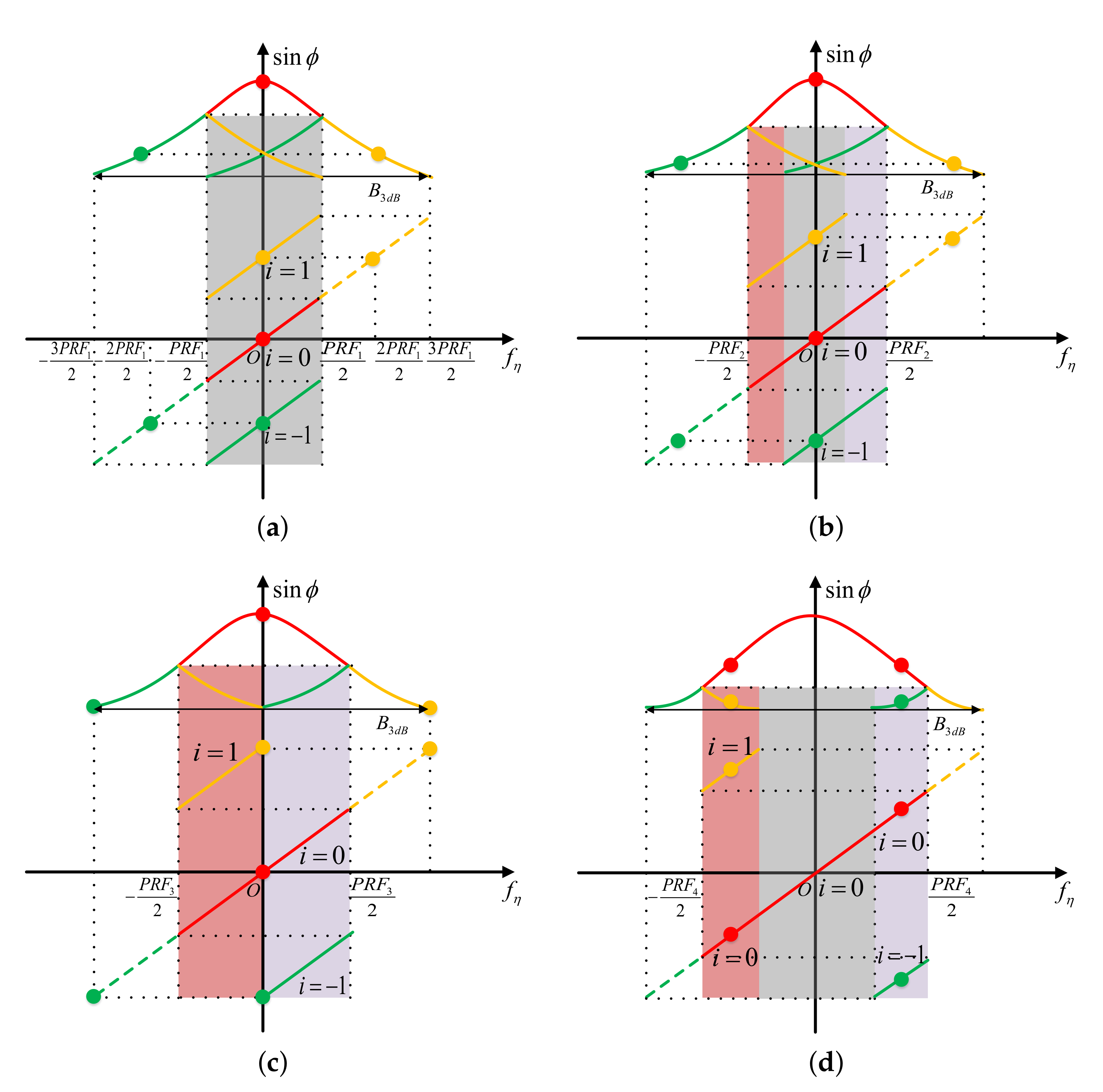
As the PRF of the multichannel SAR system is smaller than the Doppler bandwidth $B_a$, the Doppler spectrum of the echo signal received by each channel is aliased. Moreover, the PRF usually needs to be adjusted according to the beam position for different observation areas [25]. Therefore, under the influence of the PRF and Doppler centroid, the aliasing mode of the Doppler spectrum changes dynamically. Meanwhile, conventional channel calibration and signal reconstruction methods often rely heavily on the accuracy of the steering vector [17]. Thus, it is necessary to construct the practical steering matrix accurately. For simplicity, a three-channel SAR system is used in the subsequent analysis. The spatial distribution of samples of the three-channel is shown in Figure 2. Then, the Doppler spectrum of the corresponding spatial sampling distribution is shown in Figure 3. Obviously, the Doppler spectrum is a dynamic piecewise function against PRF. Equation (8) can be expressed in the following four ways.

Uniform sampling:

$$\mathit{A}\left(f_{\eta }\right)=\left[{\mathit{a}}_{-\mathit{1}}\left(f_{\eta }\right),{\mathit{a}}_{\mathbf{0}}\left(f_{\eta }\right),{\mathit{a}}_{\mathbf{1}}\left(f_{\eta }\right)\right]f_{\eta }\in D_1$$

(12)

Nonuniform sampling with spatial proximity of channels 1 and 3:

$$\begin{array}{c}\hfill \mathit{A}\left(f_{\eta }\right)=\left\{\begin{array}{cc}\left[{\mathit{a}}_{\mathbf{0}}\left(f_{\eta }\right),{\mathit{a}}_{\mathbf{1}}\left(f_{\eta }\right)\right]\hfill & f_{\eta }\in D_1\hfill \\ \left[{\mathit{a}}_{-\mathbf{1}}\left(f_{\eta }\right),{\mathit{a}}_{\mathbf{0}}\left(f_{\eta }\right),{\mathit{a}}_{\mathbf{1}}\left(f_{\eta }\right)\right]\hfill & f_{\eta }\in D_2\hfill \\ \left[{\mathit{a}}_{-\mathbf{1}}\left(f_{\eta }\right),{\mathit{a}}_{\mathbf{0}}\left(f_{\eta }\right)\right]\hfill & f_{\eta }\in D_3\hfill \end{array}\right.\end{array}$$

(13)

Nonuniform sampling with spatially coinciding samples of channels 1 and 3:

$$\begin{array}{c}\hfill \mathit{A}\left(f_{\eta }\right)=\left\{\begin{array}{cc}\left[{\mathit{a}}_{\mathbf{0}}\left(f_{\eta }\right),{\mathit{a}}_{\mathbf{1}}\left(f_{\eta }\right)\right]\hfill & f_{\eta }\in D_1\hfill \\ \left[{\mathit{a}}_{-\mathbf{1}}\left(f_{\eta }\right),{\mathit{a}}_{\mathbf{0}}\left(f_{\eta }\right)\right]\hfill & f_{\eta }\in D_3\hfill \end{array}\right.\end{array}$$

(14)

Nonuniform sampling with spatially interleaved samples of channels 1 and 3:

$$\begin{array}{c}\hfill \mathit{A}\left(f_{\eta }\right)=\left\{\begin{array}{cc}\left[{\mathit{a}}_{\mathbf{0}}\left(f_{\eta }\right),{\mathit{a}}_{\mathbf{1}}\left(f_{\eta }\right)\right]\hfill & f_{\eta }\in D_1\hfill \\ \left[{\mathit{a}}_{\mathbf{0}}\left(f_{\eta }\right)\right]\hfill & f_{\eta }\in D_2\hfill \\ \left[{\mathit{a}}_{-\mathbf{1}}\left(f_{\eta }\right),{\mathit{a}}_{\mathbf{0}}\left(f_{\eta }\right)\right]\hfill & f_{\eta }\in D_3\hfill \end{array}\right.\end{array}$$

(15)

where $D_1$, $D_2$, and $D_3$ are the independent variable ranges of the shades of gray, orange, and purple in Figure 3, respectively.

In order to verify the above conclusion from the perspective of the data domain, the capon method is used to scan the signal in the entire bandwidth. This is based on the idea of spatial filtering in array signal processing. Therefore, the new steering vector can be written as

$$\tilde{\mathit{a}}\left({\tilde{f}}_{\eta }\right)={[e^{+j\pi {\tilde{f}}_{\eta }\mathrm{\Delta }{x}_1/v_s},\cdots ,e^{+j\pi {\tilde{f}}_{\eta }\mathrm{\Delta }{x}_M/v_s}]}^T$$

(16)

where ${\tilde{f}}_{\eta }$ is the azimuth frequency, and $(-M·PR{F}_{uni})/2\le {\tilde{f}}_{\eta }\le (M·PR{F}_{uni})/2$. Here, the $PR{F}_{uni}$ satisfies the anti-DPCA condition. The capon spectrum constructed using the new steering vector can be written as [20]

$$P_{capon}({\widetilde{f_{\eta }}}_q,{f_{\eta }}_p)=\frac{1}{{\tilde{\mathit{a}}}^H\left({\widetilde{f_{\eta }}}_q\right){\mathit{R}}^{-1}\left({f_{\eta }}_p\right)\tilde{\mathit{a}}\left({\widetilde{f_{\eta }}}_q\right)}$$

(17)

where ${\widetilde{f_{\eta }}}_q$ and ${f_{\eta }}_p$ represent the frequency points within bandwidth and PRF of SAR system, respectively. The statistical covariance matrix of the echo signal at the Doppler bin $f_{\eta }$ can be expressed as

$$\begin{array}{ccc}\hfill \mathit{R}& & =\underset{\tau }{E}\left\{\mathit{S}(f_{\eta },\tau ){\mathit{S}}^H(f_{\eta },\tau )\right\}\hfill \\ & & =\mathbf{\Gamma }\left(\gamma \right)\mathit{A}·\underset{\tau }{E}\left\{{\mathit{S}}_{\mathbf{0}}(f_{\eta },\tau ){\mathit{S}}_{\mathbf{0}}^H(f_{\eta },\tau )\right\}·{\mathit{A}}^H\mathbf{\Gamma }{\left(\gamma \right)}^H+{\sigma }_n^2{\mathit{I}}_{\mathit{M}}\hfill \end{array}$$

(18)

where $\mathrm{E}\{•\}$ denotes the statistical average, ${(•)}^H$ denotes the matrix conjugate transpose operator, and ${\sigma }_n^2$ is the noise power. In practice, the statistical covariance matrix of (18) can be estimated by using the echo samples of the adjacent range bins. The sample covariance matrix $\widehat{\mathit{R}}\left(f_{\eta }\right)$ can be calculated by [4]

$$\widehat{\mathit{R}}\left(f_{\eta }\right)=\frac{1}{Nr}\sum _{k=1}^{Nr}\mathit{S}(f_{\eta },k){\mathit{S}}^H(f_{\eta },k)$$

(19)

where $Nr$ is the number of range bins used to calculate the sample covariance matrix, and $\mathit{S}(f_{\eta },k)$ represents the multichannel output vector from Doppler bin $f_{\eta }$ and range bin k.

3.2. Channel Errors Calibration

Based on the analysis above, the structure of the Doppler spectrum must be determined accurately before channel error calibration. The idea of eigendecomposition was originally used in array signal processing to determine the direction of arrival of the signal and estimate the gain-phase errors of the system at the time [26]. Furthermore, the eigendecomposition of covariance matrix $R\left(f_{\eta }\right)$ can be reformulated as follows:

$$\begin{array}{ccc}\hfill \mathit{R}\left(f_{\eta }\right)& & =\mathit{U}·\mathbf{\Sigma }·{\mathit{U}}^H\hfill \\ & & ={\mathit{U}}_{\mathit{S}}·{\mathbf{\Sigma }}_{\mathit{S}}·{\mathit{U}}_{\mathit{S}}^H+{\mathit{U}}_{\mathit{N}}·{\mathbf{\Sigma }}_{\mathit{N}}·{\mathit{U}}_{\mathit{N}}^H\hfill \end{array}$$

(20)

In the spaceborne SAR system, the eigenvalues can be acquired in descending order $({\lambda }_1>{\lambda }_2>\cdots >{\lambda }_{2I+1}\gg {\lambda }_{2I+2}=\cdots ={\lambda }_M={\sigma }_n^2)$ by decomposing the covariance matrix. In order to satisfy Nyquist sampling theorem $(M·PRF\ge (2I+1)PRF>B_a)$, there must be redundant channels. Where $\mathbf{\Sigma }=diag[{\lambda }_1\cdots {\lambda }_i\cdots {\lambda }_M]$, corresponding to $\mathit{U}=[{\mathit{u}}_{\mathbf{1}}\cdots {\mathit{u}}_{\mathit{i}}\cdots {\mathit{u}}_{\mathit{M}}]$. ${\mathit{U}}_{\mathit{S}}$ is the $M\times (2I+1)$ signal subspace matrix spanned by the eigenvectors corresponding to the $(2I+1)$ largest eigenvalues, while ${\mathit{U}}_{\mathit{N}}$ is the $M\times (M-(2I+1\left)\right)$ noise subspace matrix spanned by the eigenvectors corresponding to the $(M-(2I+1\left)\right)$ smallest eigenvalues. As the space spanned by the signal subspace ${\mathit{U}}_{\mathit{S}}$ is the same as the space spanned by the steering matrix $\mathbf{\Gamma }\left(\mathit{\gamma }\right)\mathit{A}$, there exists a unique non-singular matrix $\mathit{T}$ that satisfies

$${\mathit{U}}_{\mathit{S}}=\mathbf{\Gamma }\left(\mathit{\gamma }\right)\mathit{A}\left(f_{\eta }\right)\mathit{T}$$

(21)

As the $\mathbf{\Gamma }\left(\mathit{\gamma }\right)$ is non-singular matrix, for the convenience of subsequent processing, Equation (21) can be reformulated as follows:

$$\mathbf{\Gamma }\left(\overline{\mathit{\gamma }}\right){\mathit{U}}_{\mathit{S}}=\mathit{A}\left(f_{\eta }\right)\mathit{T}$$

(22)

where $\mathbf{\Gamma }\left(\overline{\mathit{\gamma }}\right)={\mathbf{\Gamma }}^{-1}\left(\mathit{\gamma }\right)=diag\{\overline{{\gamma }_1},\cdots ,\overline{{\gamma }_i},\cdots ,\overline{{\gamma }_M}\}$ and the vector $\overline{\mathit{\gamma }}$ can be written as

$$\overline{\mathit{\gamma }}={[{\rho }_1^{-1}{e}^{-j{\xi }_1},\cdots ,{\rho }_i^{-1}{e}^{-j{\xi }_i},\cdots ,{\rho }_M^{-1}{e}^{-j{\xi }_M}]}^T$$

(23)

In the presence of noise, the least square solution of the non-singular matrix $\mathit{T}$ is estimated by solving the following optimization problem:

$$\begin{array}{ccc}& & \underset{\widehat{\mathit{T}},\overline{\mathit{\gamma }}}{\min }{∥\mathbf{\Gamma }\left(\overline{\mathit{\gamma }}\right){\mathit{U}}_{\mathit{S}}-\mathit{A}\left(f_{\eta }\right)\widehat{\mathit{T}}∥}_F^2\hfill \\ & & \mathrm{s}.\mathrm{t}.{\mathit{\omega }}^H\overline{\mathit{\gamma }}=1\hfill \end{array}$$

(24)

where ${∥•∥}_F^2$ denotes the square of the Frobenius norm. Without loss of generality, the middle channel can be set as the reference channel, and $\mathit{\omega }={[0,\cdots ,0,1,0,\cdots ,0]}^T$ is an $M\times 1$ vector. The least squares solution of $\widehat{\mathit{T}}$ is written as

$$\widehat{\mathbf{T}}={\left({\mathit{A}}^H\left(f_{\eta }\right)\mathit{A}\left(f_{\eta }\right)\right)}^{-1}{\mathit{A}}^H\left(f_{\eta }\right)\mathbf{\Gamma }\left(\overline{\mathit{\gamma }}\right){\mathit{U}}_{\mathit{S}}$$

(25)

Substitute Equation (25) into Equation (24), the optimization problem in Equation (24) can be reformulated as follows:

$$\begin{array}{ccc}& & \underset{\overline{\mathit{\gamma }}}{\min }tr\left\{{\mathit{U}}_{\mathit{S}}{\mathit{U}}_{\mathit{S}}^H{\mathbf{\Gamma }}^H\left(\overline{\mathit{\gamma }}\right){\mathit{P}}_{\mathit{A}}^{\perp }\left(f_{\eta }\right)\mathbf{\Gamma }\left(\overline{\mathit{\gamma }}\right)\right\}\hfill \\ & & \mathrm{s}.\mathrm{t}.{\mathit{\omega }}^H\overline{\mathit{\gamma }}=1\hfill \end{array}$$

(26)

where ${\mathit{P}}_{\mathit{A}}^{\perp }\left(f_{\eta }\right)$ denotes a matrix that is orthogonal to the projection matrix of $\mathit{A}$, and $tr\{•\}$ represents the trace of a matrix. After some detailed derivation as shown in the Appendix A, Equation (26) can be finally rewritten as

$$\begin{array}{ccc}& & \underset{\overline{\mathit{\gamma }}}{\min }{\overline{\mathit{\gamma }}}^H\mathit{G}\left(f_{\eta }\right)\overline{\mathit{\gamma }}\hfill \\ & & \mathrm{s}.\mathrm{t}.{\mathit{\omega }}^H\overline{\mathit{\gamma }}=1\hfill \end{array}$$

(27)

where $\mathit{G}\left(f_{\eta }\right)={\left({\mathit{U}}_{\mathit{S}}{\mathit{U}}_{\mathit{S}}^H\right)}^T\circ {\mathit{P}}_{\mathit{A}}^{\perp }\left(f_{\eta }\right)$ is an $(M\times M)$ Hermitian matrix, and ∘ denotes the Hadamard product.

By applying Lagrange multiplier method, we define a new function associated with Equation (27) as follows:

$$L(\overline{\mathit{\gamma }},\mu )={\overline{\mathit{\gamma }}}^H\mathit{G}\left(f_{\eta }\right)\overline{\mathit{\gamma }}+\mu ({\mathit{\omega }}^H\overline{\mathit{\gamma }}-1)$$

(28)

where $\mu$ is the Lagrange multiplier. To calculate the stationary points, we differentiate $L(\overline{\mathit{\gamma }},\mu )$ with respect to $\overline{\mathit{\gamma }}$ and $\mu$. By setting these partial derivatives equal to zero, the Lagrange multiplier can be obtained as $\mu =2{\left({\mathit{\omega }}^H{\mathit{G}}^{-1}\left(f_{\eta }\right)\mathit{\omega }\right)}^{-1}$. Finally, the optimal solution can be expressed as follows:

$${\widehat{\overline{\mathit{\gamma }}}}_{f_{\eta }}={\mathit{G}}^{-1}\left(f_{\eta }\right)\mathit{\omega }{\left({\mathit{\omega }}^H{\mathit{G}}^{-1}\left(f_{\eta }\right)\mathit{\omega }\right)}^{-1}$$

(29)

Thus, the gain and phase errors between the mth channel and the reference channel can be calculated by

$${\widehat{\rho }}_{f_{\eta },m}=abs\{1/{\widehat{\overline{\mathit{\gamma }}}}_{f_{\eta }}\left(m\right)\},m=1,2,\cdots ,M.$$

(30)

$${\widehat{\xi }}_{f_{\eta },m}=angle\{1/{\widehat{\overline{\mathbf{\gamma }}}}_{f_{\eta }}\left(m\right)\},m=1,2,\cdots ,M.$$

(31)

where $abs\{•\}$ denotes the modulus of a complex number and $angle\{•\}$ represents the phase of a complex number.

According to the Doppler spectrum obtained in Equation (17), the Doppler bin with redundant space is selected. Then, the gain and phase errors estimated on these Doppler bins are averaged. Moreover, the final channel errors can be obtained:

$${\overline{\rho }}_m=\frac{1}{N}\sum _{f_{\eta ,i}=f_{\eta ,1}}^{f_{\eta ,N}}{\widehat{\rho }}_{f_{\eta ,i},m},m=1,2,\cdots ,M.$$

(32)

$${\overline{\xi }}_m=\frac{1}{N}\sum _{f_{\eta ,i}=f_{\eta ,1}}^{f_{\eta ,N}}{\widehat{\xi }}_{f_{\eta ,i},m},m=1,2,\cdots ,M.$$

(33)

where N indicates the number of redundant Doppler bins. Based on the channel error estimated above, the calibrated echo signal can be further expressed as

$$S_m^{\prime }(f_{\eta },\tau )=\frac{1}{{\overline{\rho }}_m}{S}_m(f_{\eta },\tau )e^{-j{\overline{\xi }}_m},m=1,2,\cdots ,M.$$

(34)

where $S_m^{\prime }(f_{\eta },\tau )$ denotes the signal after the gain-phase error of the mth channel is calibrated.

Besides, the necessary condition for the existence of Equation (29) is that the matrix $\mathit{G}\left(f_{\eta }\right)$ is the full rank. However, in practical applications, the matrix $\mathit{G}\left(f_{\eta }\right)$ in some Doppler bins is close to the singular value, making the results may not be accurate. Therefore, the diagonal loading method was considered [27,28]. Then, we have

$$\tilde{\mathit{G}}\left(f_{\eta }\right)=\mathit{G}\left(f_{\eta }\right)+\delta \mathit{I}$$

(35)

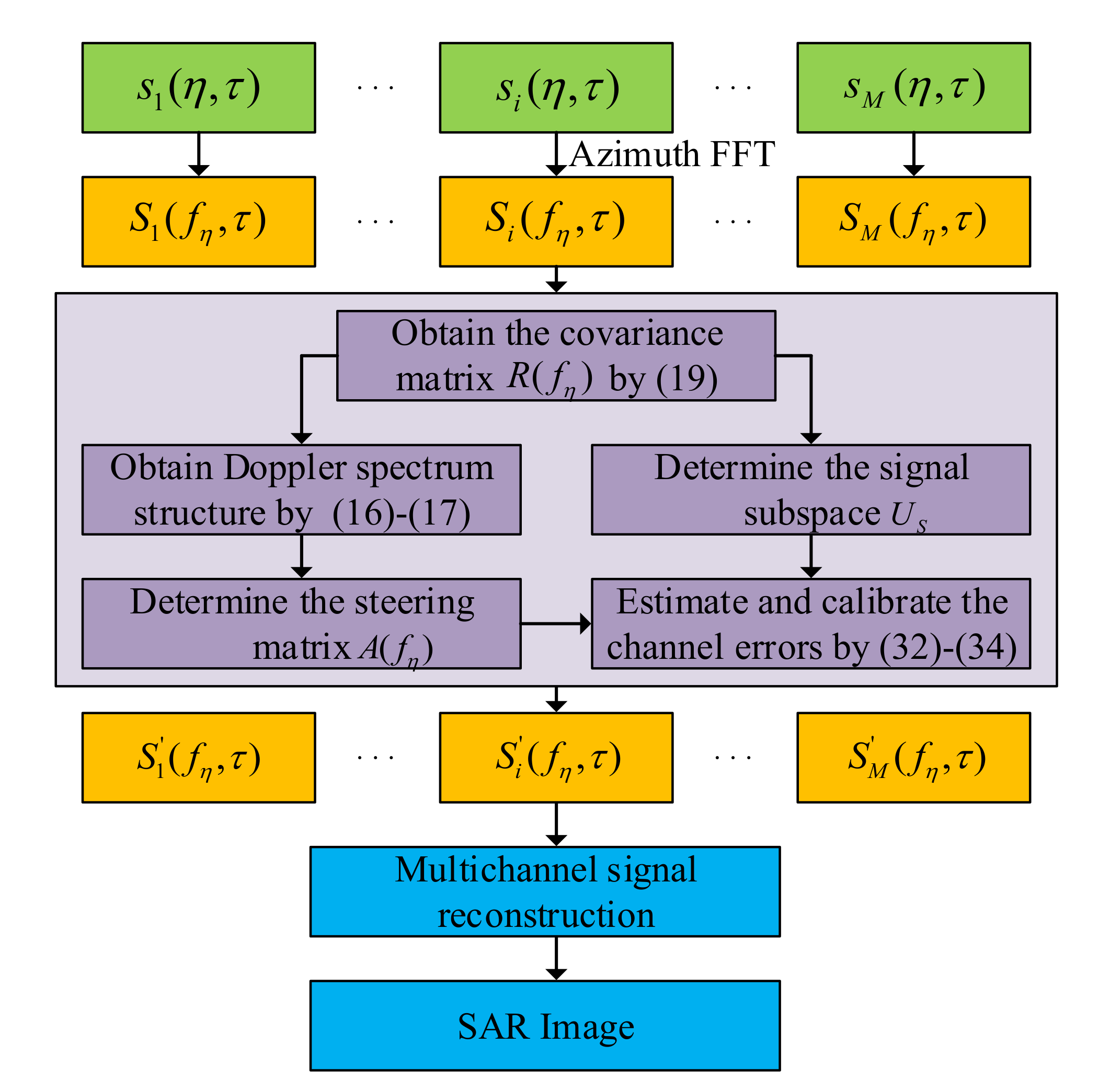
Equation (33) guarantees that the matrix $\mathit{G}\left(f_{\eta }\right)$ is invertible. Here, $\delta$ is a diagonal loading factor. Without loss of generality, $\delta$ is usually chosen as a small value. Finally, after the channel errors are compensated, the azimuth signal can be effectively reconstructed by the DBF or the STAP method. Based on the above analysis, the main steps of the algorithm based on the proposed method can be defined. The flow chart of the algorithm is shown in Figure 4.

Step 1: Carry out azimuth fast Fourier transform for each channel data.

Step 2: Estimate covariance matrix $\widehat{\mathit{R}}\left(f_{\eta }\right)$ of each Doppler bin by Equation (19).

Step 3: Obtain Doppler spectrum structure by Equations (16) and (17) and determine index of ambiguity of each Doppler bin.

Step 4: Obtain the signal subspace ${\mathit{U}}_S$ by decomposing $\widehat{\mathit{R}}\left(f_{\eta }\right)$ and determine the steering matrix $\mathit{A}\left(f_{\eta }\right)$.

Step 5: Estimate the gain and phase errors by Equations (32) and (33) and calibrate the channel errors by Equation (34).

Step 6: Reconstruct signal using the DBF or STAP method.

Step 7: Obtain the unambiguous image by a conventional imaging algorithm.

4. Experiments

In this section, five-channel simulations are carried out. By adding the known phase error to each channel in advance, the estimated results of the channel phase error can be compared with true values. The performance of the proposed method is evaluated by comparison with the conventional methods. In addition, the real data acquired by the GF-3 dual-channel SAR system are processed to verify the effectiveness of the proposed method.

4.1. Simulated Data

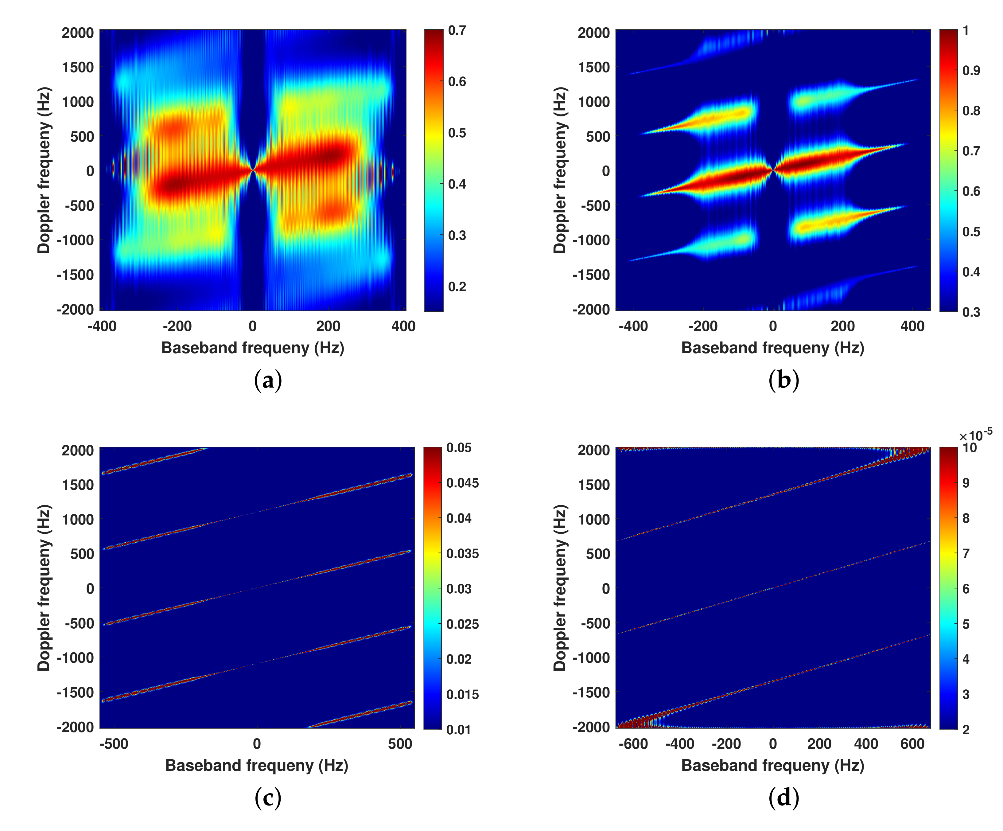
The parameters of the five-channel SAR system are listed in

Table 1. Main parameters of the simulated data.

Parameter	Symbol	Value
Wavelength	$\lambda$	0.055517 m
PRF	$f_p$	1015 Hz
Sampling rate	$f_s$	133.33 MHz
Signal bandwidth	$B_r$	100 MHz
Pulse duration	$T_r$	54.99 $\mathsf{\mu }$s
Platform velocity	$v_s$	7614 m/s
Look-angle	$\theta$	35.41
Channel number	M	5
Adjacent Channel Interval	d	3.75 m

. The SAR data are sampled at $PRF=813\mathrm{Hz}$, $PRF=903\mathrm{Hz}$, $PRF=1100\mathrm{Hz}$, and $PRF=1357\mathrm{Hz}$, respectively. Then, their Doppler spectrums are observed. It can be seen that the index of ambiguity is different for different PRFs, such as $i=-2,-1,0,1,2$ in Figure 5a, $i=-1,0,1,2$ on the left side of Figure 5b, $i=-2,-1,0,1$ on the right side of Figure 5b, and $i=-1,0,1$ in Figure 5d.

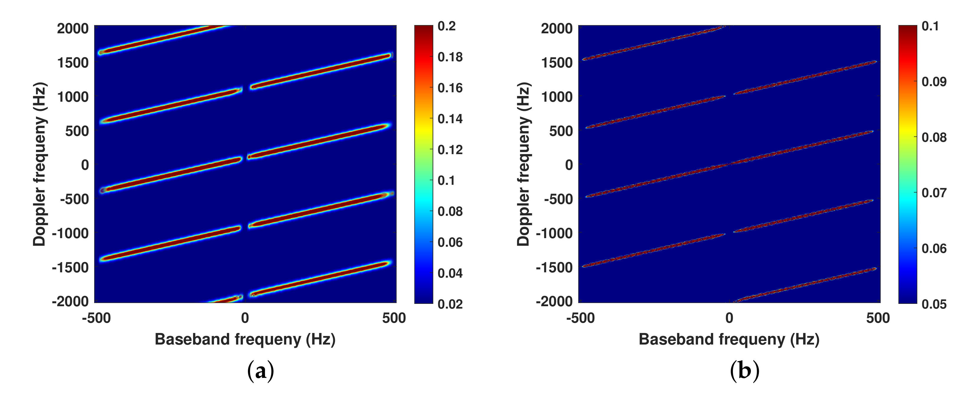
Therefore, before the phase error estimation, the steering matrix $\mathit{A}\left(f_{\eta }\right)$ of each Doppler bin must be constructed accurately according to the specific index of ambiguity. In addition, the phase errors are added to the five-channel SAR system as follows: 45°, 21°, 0°, 113°, and 78°. The influence of the channel phase errors on the Doppler spectrum is manifested by the frequency shift, as shown in Figure 6, which implies that the phase errors have basically no effect on observing the index of ambiguity using the Doppler spectrum. This is the reason for the mismatch of the reconstruction filter and the appearance of false targets in pairs in the subsequent processing.

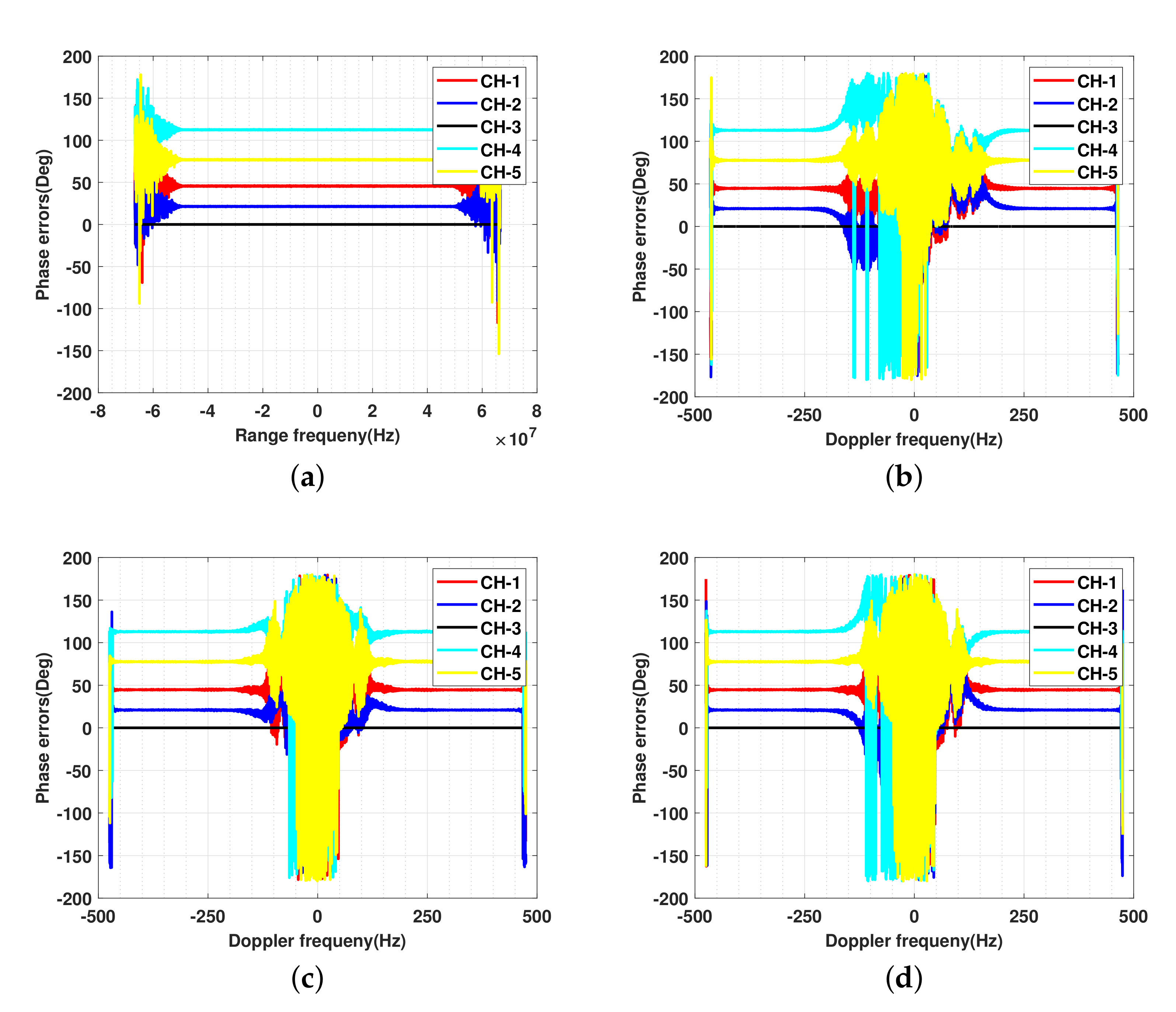
The third channel is used as the reference channel. The curves of the channel phase error are calculated by using the proposed method and the conventional methods, respectively, as shown in Figure 7. Moreover, the phase error results estimated by conventional methods and the proposed method are shown in

Table 2. Estimation results of conventional methods and proposed method with different SNRs.

Channel Number	Real Phase Error	SNR	TDCM	OSM	SSCM	MVDR	Proposed Method
Channel 1	45°	10 dB	45.5871°	44.4693°	44.5184°	44.5157°	44.7129°
		20 dB	45.6034°	44.7021°	44.6971°	44.7012°	44.7366°
		30 dB	45.6128°	44.7176°	44.7036°	44.7157°	44.7483°
Channel 2	21°	10 dB	21.3586°	20.6864°	20.7473°	21.2746°	20.8157°
		20 dB	21.3680°	20.9492°	20.9427°	21.1582°	20.9543°
		30 dB	21.3738°	21.0033°	20.9802°	20.9665°	20.9856°
Channel 3	0°	10 dB	0.0°	0.0°	0.0°	0.0°	0.0°
		20 dB	0.0°	0.0°	0.0°	0.0°	0.0°
		30 dB	0.0°	0.0°	0.0°	0.0°	0.0°
Channel 4	113°	10 dB	112.4815°	112.6456°	112.7573°	111.3848°	112.8615°
		20 dB	112.4831°	112.9002°	112.8991°	112.7977°	112.9169°
		30 dB	112.4858°	113.0129°	112.9798°	112.8825°	112.9813°
Channel 5	78°	10 dB	76.8194°	77.3443°	77.4197°	77.4258°	77.5375°
		20 dB	76.8350°	77.6058°	77.6123°	77.6077°	77.6999°
		30 dB	76.8416°	77.6395°	77.6314°	77.6425°	77.7244°

with different SNRs. It is obvious that the channel phase error estimated by the proposed method is more accurate than estimations of the TDCM, OSM, SSCM, and MDVR. Because the proposed method does not depend on the accuracy of the Doppler centroid and can precisely construct the unique non-singular matrix $\mathit{T}$.

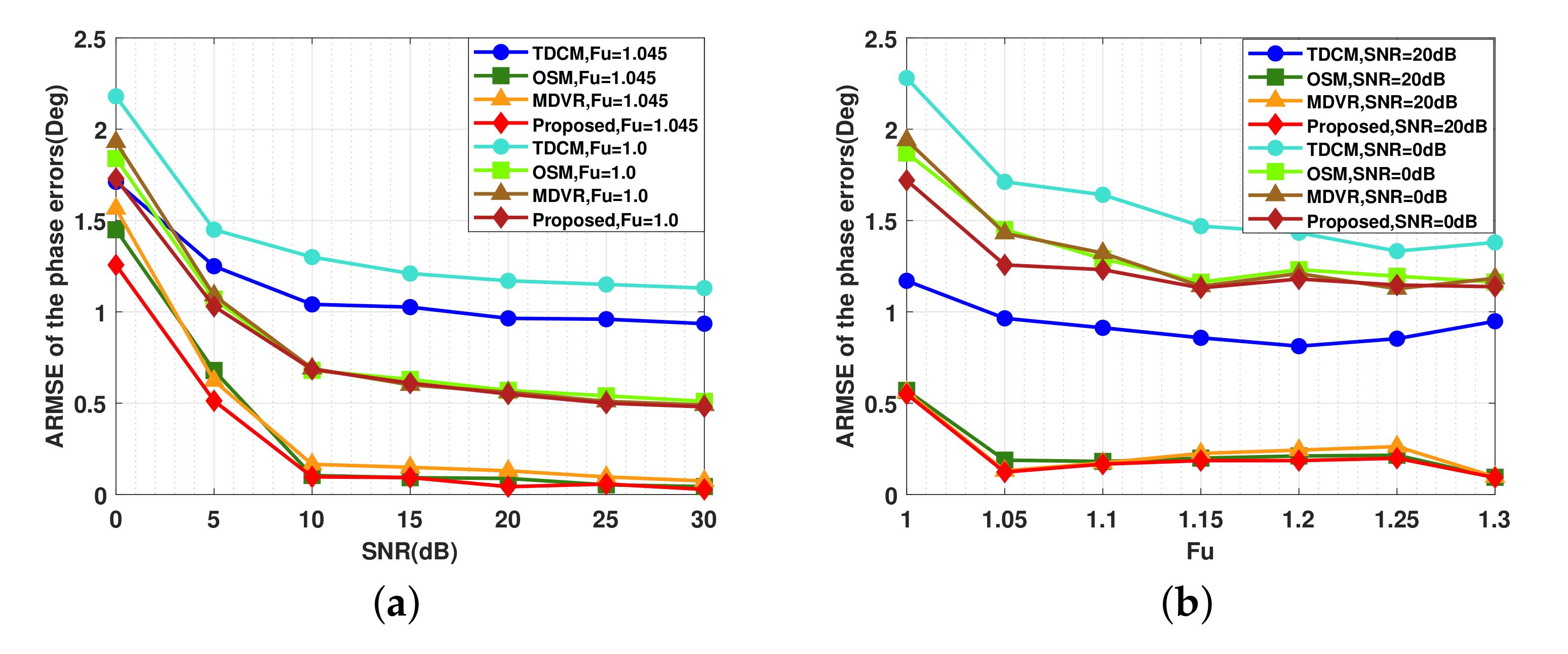
To further verify performance of the method, Monte Carlo trials based on 200 runs are conducted. Then, the phase errors added to the five-channel SAR system are uniformly distributed in $[-\pi ,\pi ]$. The average root mean square error (ARMSE) of phase errors estimation versus SNR and the uniformity factor $Fu$ [29] are used to evaluate the performance of the proposed calibration method compared with the conventional TDCM, OSM, and MDVR. Here, $F_u$ is defined as the ratio of $d/2$ to $vs/(M·PRF)$. From the result shown in Figure 8a, it is clear that the proposed method has higher accuracy than the TDCM, the OSM and the MDVR versus SNR, especially in regard to low SNRs. In addition, the proposed method is more robust than the TDCM, the OSM and the MDVR versus the uniformity factor $Fu$, especially in the case of high non-uniformity (see Figure 8b).

4.2. Real Data

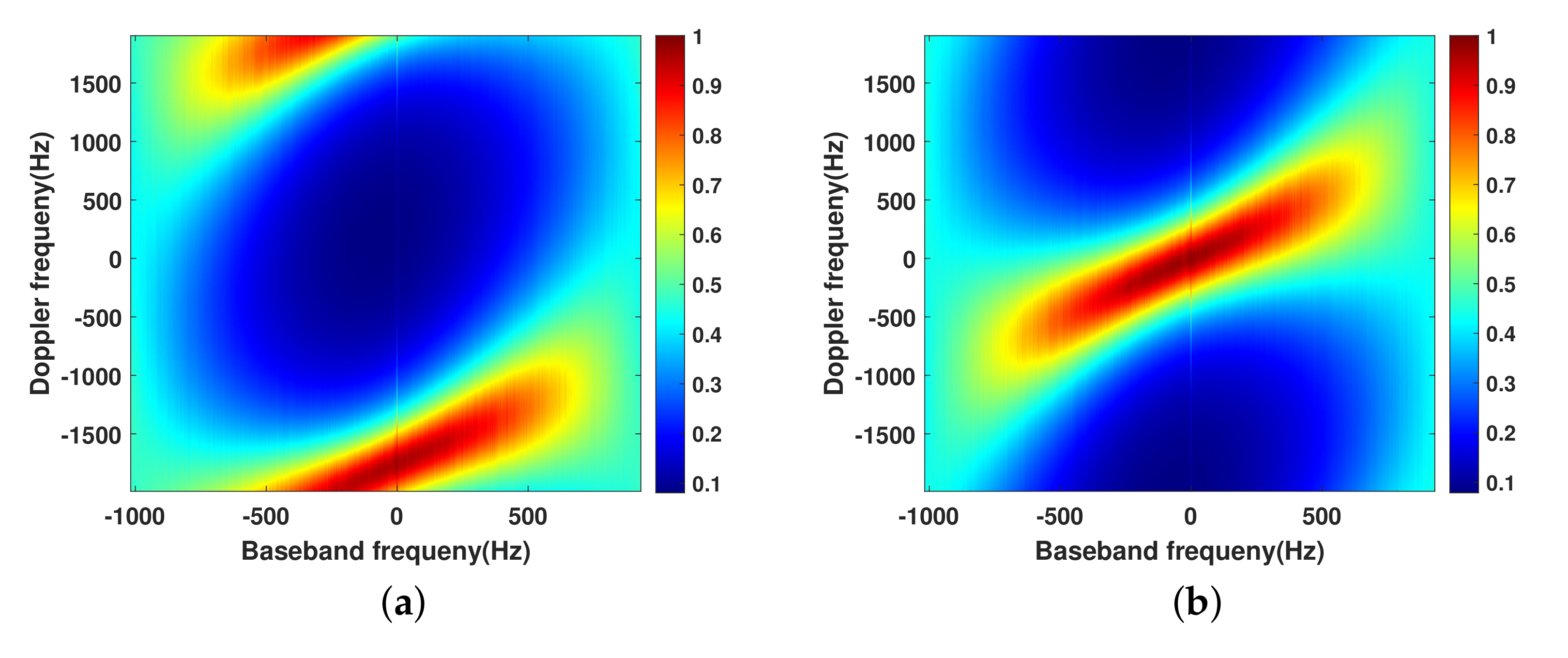
In this experiment with dual-channel GF-3 SAR data, the performance of the proposed calibration method is evaluated in comparison with the TDCM, OSM, and MVDR. The system works in the C-band, with a satellite speed of approximately 7480 m/s and a Doppler bandwidth of approximately 3534 Hz. At the same time, the azimuth sampling is achieved only at the PRF of 1948 Hz, so the uniformity factor $Fu$ is approximately 0.9766. The Doppler spectrum is observed before and after the channel phase error calibration. From the results shown in Figure 9, the GF-3 dual-channel SAR system is nearly uniformly sampled and the channel phase error has a great influence on the Doppler spectrum. Therefore, the steering matrix $\mathit{A}\left(f_{\eta }\right)$ of each Doppler bin needs to be adjusted in time according to the index of ambiguity. As shown in Figure 9a, under the weighting of the antenna pattern, the energy is mainly concentrated in the subspace spanned by the steering vector ${\mathit{a}}_{\mathbf{0}}\left(f_{\eta }\right)$. Thus, in the following processing, the steering matrix $\mathit{A}\left(f_{\eta }\right)={\mathit{a}}_{\mathbf{0}}\left(f_{\eta }\right)$ is applied.

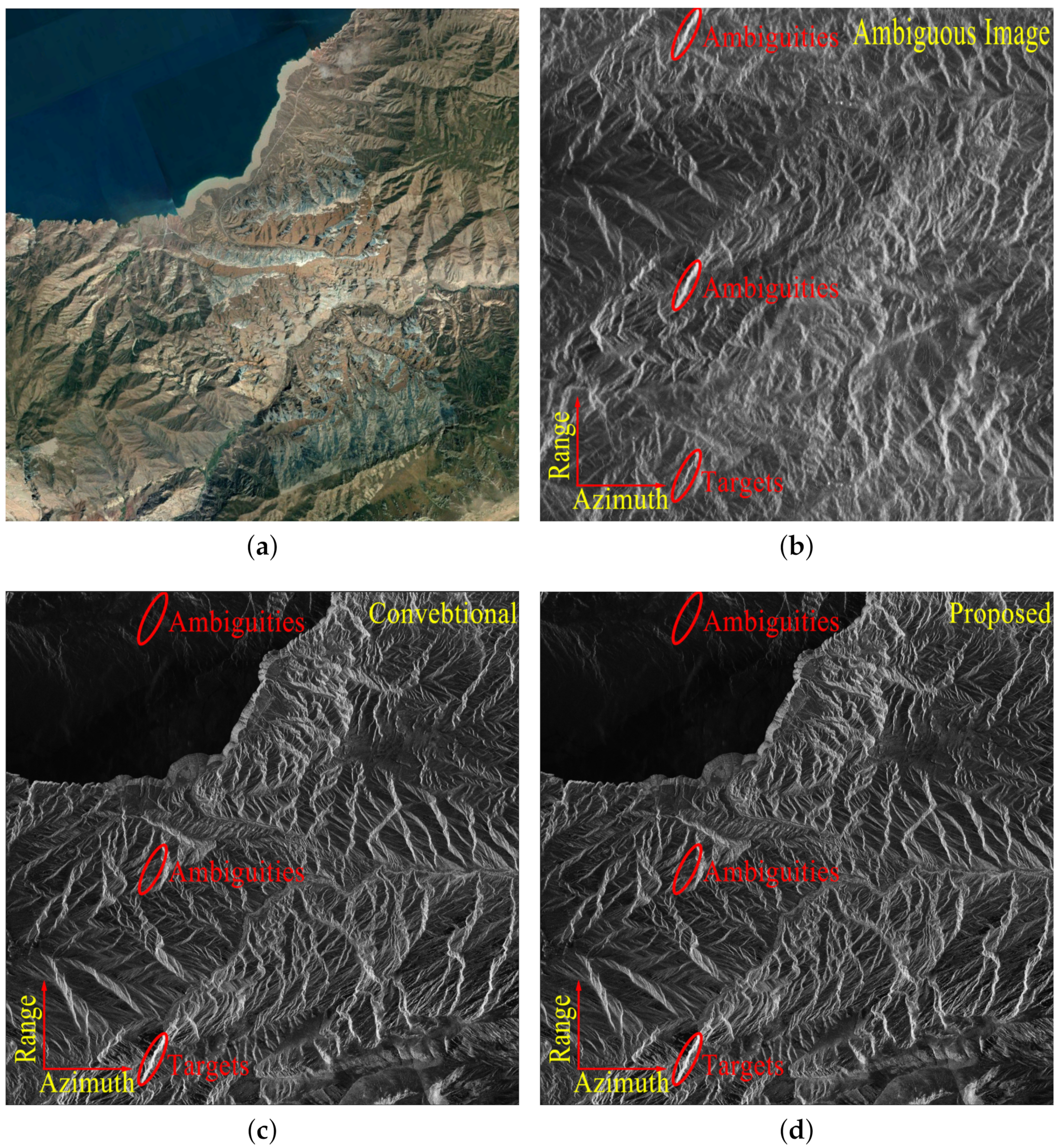
Due to the weak scattering of the sea surface, there is more obvious azimuth ambiguity at the boundary between land and sea, as shown in Figure 10b. Obviously, performing HRWS reconstruction directly before channel phase error calibration will result in false targets in pairs. The CH-1 is the reference channel, and the CH-2 is the channel to be calibrated. The curve of the channel gain error is calculated by using the method proposed in this paper, as shown in Figure 11a. As can be seen in Figure 11b, the spectrum of CH-2 is larger than that of CH-1, and it is clear that, after the gain error calibration, the CH-2 coincides with the signal of the CH-1. The above analysis also verifies the effectiveness of the proposed method in gain calibration.

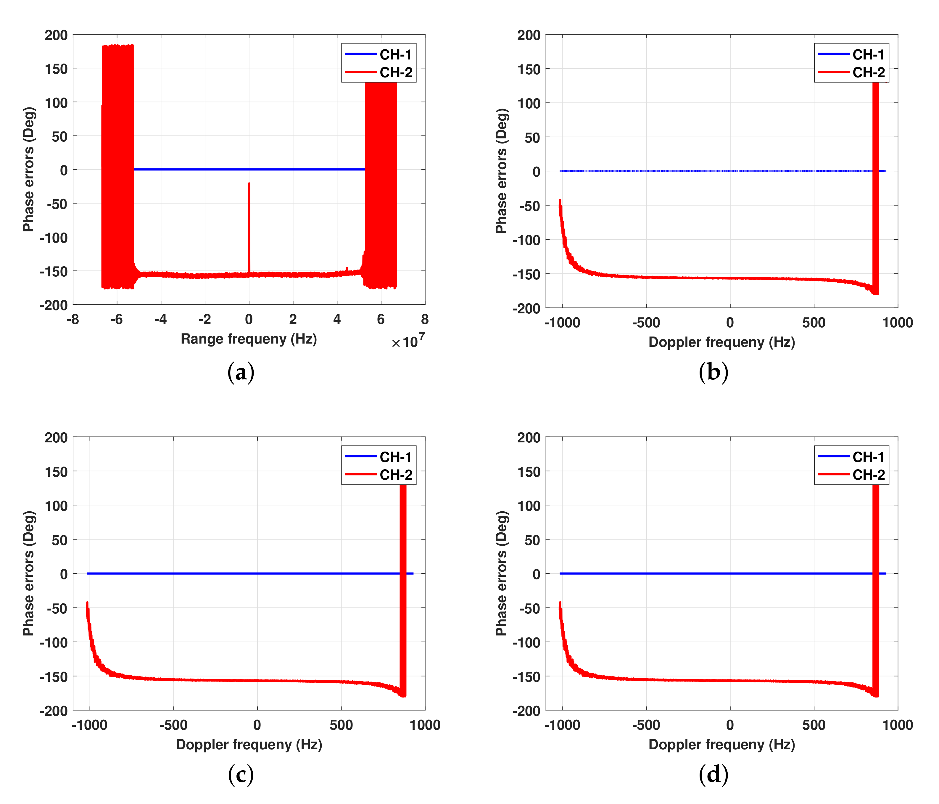
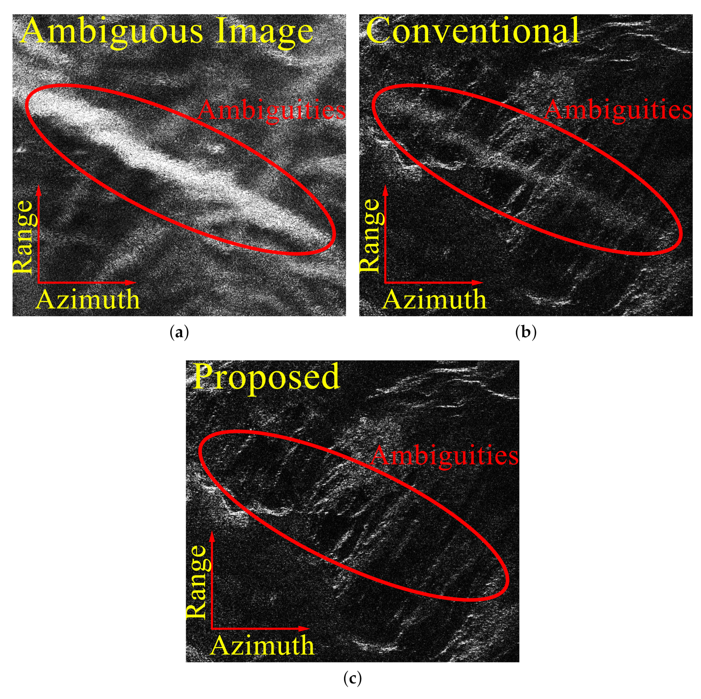
The curve of the channel phase error is calculated by using the proposed method and the conventional methods, respectively, as shown in Figure 12. It is obvious that the channel phase error is basically stable during the entire operation of the satellite. In addition, the average phase errors estimated by the proposed method, TDCM, OSM, and MDVR are −156.9447°, −154.0712°, −156.2613°, and −156.1321°, respectively. As shown in Figure 13a, the phase errors of some Doppler bins estimated by the OSM are ill-conditioned. The proposed method successfully overcomes the shortcoming by using the diagonal loading technique, as shown in Figure 13b. Then, after the gain-phase error is compensated and the non-uniform signal is reconstructed, the unambiguous image can be obtained by a conventional imaging algorithm. Figure 10a shows the corresponding optical image. Figure 10c,d shows the imaging results using TDCM and the proposed method, respectively. Magnified images of the results of the different calibration methods for strong scatters are shown in Figure 14, including the TDCM and the proposed method. It is obvious that the proposed method can effectively calibrate channel phase errors and improve the image quality.

5. Discussion

In Section 4, the proposed method has been confirmed by processing the simulations of the five-channel system and the real data acquired by the GF-3 dual-channel. As shown in Figure 5, it is crucial to adjust the steering matrix $\mathit{A}\left(f_{\eta }\right)$ of each Doppler bin in time through the Doppler spectrum. Figure 8a demonstrates that the proposed method has higher accuracy than the TDCM, the OSM and the MDVR versus SNR, especially in regard to low SNRs. Meanwhile, compared with the conventional methods, the proposed method is more robust versus the uniformity factor $Fu$, as shown in Figure 8b, especially in the case of high non-uniformity. For the OSM, when the PRF is close to the anti-DPCA condition $(Fu=1)$ [25], there are not enough redundant channels to construct the signal subspace. Moreover, the MVDR only maintains the gain of the desired signal constant, neglecting to suppress the unwanted signal, which will significantly affect the performance. The result of the proposed method is a closed-form expression, contrary to the result of the method presented in [17], which will greatly reduce the computational load due to the need for iteration.

The imaging results of the real data acquired by the GF-3 dual-channel system, shown in Figure 10, indicate that the proposed method has better performance than the TDCM method, as the proposed method does not depend on the accuracy of the Doppler centroid. Moreover, as the number of channels increases, the correlation between adjacent channels decreases and the channel phase errors accumulate. The proposed method eliminates the phase error accumulation, because the phase error between each channel and the reference channel is directly calculated. The phase errors of some Doppler bins estimated by OSM are ill-conditioned. Because, under the condition of large samples, the matrices $(\sum {\mathrm{\Gamma }}^H{a}_i^H{U}_N{U}_N^H{a}_i\mathrm{\Gamma })$ of some Doppler bins are close to singular values, which will lead to the possibility of its inverse matrix being ill-conditioned. Averaging the estimated results of the phase error may be inaccurate due to these ill-conditioned values. As shown in Figure 13, the diagonal loading technology can successfully overcome the shortcoming.

6. Conclusions

A novel channel error calibration algorithm for the multichannel in the azimuth HRWS SAR system is presented. Prior to the channel error estimation, the steering matrix $\mathit{A}\left(f_{\eta }\right)$ of each Doppler bin can be adjusted in time according to the Doppler spectrum. This will greatly improve the accuracy of phase error estimation. The proposed method is based on the idea of minimizing the mean square error between the signal subspace and the space spanned by the practical steering vectors. Compared with the TDCM, the proposed method no longer depends on the accuracy of the Doppler centroid estimation. In addition, the proposed method is more stable than the OSM as it uses the diagonal loading technique compared with OSM. Moreover, compared with the OSM, there is no restriction on redundant channels. In the performance evaluation, the simulation results and real data processing demonstrate that the proposed method has higher accuracy and robustness than the conventional methods, especially in the case of low SNRs and the case of high non-uniformity.

References

- Krieger, G.; Gebert, N.; Moreira, A. Unambiguous SAR signal reconstruction from nonuniform displaced phase center sampling. IEEE Geosci. Remote Sens. Lett. 2004, 1, 260–264. [Google Scholar] [CrossRef] [Green Version]
- Gebert, N.; Krieger, G.; Moreira, A. Digital beamforming on receive: Techniques and optimization strategies for high-resolution wide-swath SAR imaging. IEEE Trans. Aerosp. Electron. Syst. 2009, 45, 564–592. [Google Scholar] [CrossRef] [Green Version]
- Krieger, G.; Gebert, N.; Moreira, A. SAR signal reconstruction from non-uniform displaced phase centre sampling. In Proceedings of the 2004 IEEE International Geoscience and Remote Sensing Symposium (IGARSS 2004), Anchorage, AK, USA, 20–24 September 2004; Volume 3, pp. 1763–1766. [Google Scholar]
- Li, Z.; Wang, H.; Su, T.; Bao, Z. Generation of wide-swath and high-resolution SAR images from multichannel small spaceborne SAR systems. IEEE Geosci. Remote Sens. Lett. 2005, 2, 82–86. [Google Scholar] [CrossRef]
- Kim, J.H.; Younis, M.; Prats-Iraola, P.; Gabele, M.; Krieger, G. First spaceborne demonstration of digital beamforming for azimuth ambiguity suppression. IEEE Trans. Geosci. Remote Sens. 2012, 51, 579–590. [Google Scholar] [CrossRef] [Green Version]
- Renyuan, C.; Kai, J.; Yanmei, Y.; Changyao, Z. High resolution dual channel receiving SAR compensation technique. In Proceedings of the 2007 1st Asian and Pacific Conference on Synthetic Aperture Radar, Huangshan, China, 5–9 November 2007; pp. 713–717. [Google Scholar]
- Feng, J.; Gao, C.; Zhang, Y.; Wang, R. Phase mismatch calibration of the multichannel SAR based on azimuth cross correlation. IEEE Geosci. Remote Sens. Lett. 2012, 10, 903–907. [Google Scholar] [CrossRef]
- Fang, C.; Liu, Y.; Suo, Z.; Li, Z.; Chen, J. Improved channel mismatch estimation for multi-channel HRWS SAR based on azimuth cross-correlation. Electron. Lett. 2018, 54, 235–237. [Google Scholar] [CrossRef]
- Shang, M.; Qiu, X.; Han, B.; Ding, C.; Hu, Y. Channel imbalances and along-track baseline estimation for the GF-3 azimuth multichannel mode. Remote Sens. 2019, 11, 1297. [Google Scholar] [CrossRef] [Green Version]
- Li, Z.; Bao, Z.; Wang, H.; Liao, G. Performance improvement for constellation SAR using signal processing techniques. IEEE Trans. Aerosp. Electron. Syst. 2006, 42, 436–452. [Google Scholar]
- Zhang, L.; Xing, M.D.; Qiu, C.W.; Bao, Z. Adaptive two-step calibration for high-resolution and wide-swath SAR imaging. IET Radar Sonar Navig. 2010, 4, 548–559. [Google Scholar] [CrossRef]
- Guo, X.; Gao, Y.; Wang, K.; Liu, X. Improved channel error calibration algorithm for azimuth multichannel SAR systems. IEEE Geosci. Remote Sens. Lett. 2016, 13, 1022–1026. [Google Scholar] [CrossRef]
- Yang, T.; Li, Z.; Liu, Y.; Bao, Z. Channel error estimation methods for multichannel SAR systems in azimuth. IEEE Geosci. Remote Sens. Lett. 2012, 10, 548–552. [Google Scholar] [CrossRef]
- Yang, T.; Li, Z.; Liu, Y.; Suo, Z.; Bao, Z. Channel error estimation methods for multi-channel HRWS SAR systems. In Proceedings of the 2013 IEEE International Geoscience and Remote Sensing Symposium-IGARSS, Melbourne, Australia, 21–26 July 2013; pp. 4507–4510. [Google Scholar]
- Liu, A.; Liao, G.; Ma, L.; Xu, Q. An array error estimation method for constellation SAR systems. IEEE Geosci. Remote Sens. Lett. 2010, 7, 731–735. [Google Scholar] [CrossRef]
- Xu, Q.; Liao, G.; Liu, A.; Zhang, J. Self-calibration method without joint iteration for distributed small satellite SAR systems. EURASIP J. Adv. Signal Process. 2013, 2013, 31. [Google Scholar] [CrossRef] [Green Version]
- Zhou, Y.; Wang, R.; Deng, Y.; Yu, W.; Fan, H.; Liang, D.; Zhao, Q. A novel approach to Doppler centroid and channel errors estimation in azimuth multi-channel SAR. IEEE Trans. Geosci. Remote Sens. 2019, 57, 8430–8444. [Google Scholar] [CrossRef]
- Zhang, L.; Gao, Y.; Liu, X. Robust channel phase error calibration algorithm for multichannel high-resolution and wide-swath SAR imaging. IEEE Geosci. Remote Sens. Lett. 2017, 14, 649–653. [Google Scholar] [CrossRef]
- Huang, H.; Huang, P.; Liu, X.; Xia, X.G.; Deng, Y.; Fan, H.; Liao, G. A Novel Channel Errors Calibration Algorithm for Multichannel High-Resolution and Wide-Swath SAR Imaging. IEEE Trans. Geosci. Remote Sens. 2021. [Google Scholar] [CrossRef]
- Zuo, S.S.; Xing, M.; Xia, X.G.; Sun, G.C. Improved signal reconstruction algorithm for multichannel SAR based on the Doppler spectrum estimation. IEEE J. Sel. Top. Appl. Earth Obs. Remote Sens. 2016, 10, 1425–1442. [Google Scholar] [CrossRef]
- Moreira, A.; Mittermayer, J.; Scheiber, R. Extended chirp scaling algorithm for air-and spaceborne SAR data processing in stripmap and ScanSAR imaging modes. IEEE Trans. Geosci. Remote Sens. 1996, 34, 1123–1136. [Google Scholar] [CrossRef]
- Raney, R.K.; Runge, H.; Bamler, R.; Cumming, I.G.; Wong, F.H. Precision SAR processing using chirp scaling. IEEE Trans. Geosci. Remote Sens. 1994, 32, 786–799. [Google Scholar] [CrossRef]
- Liang, D.; Wang, R.; Deng, Y.; Fan, H.; Zhang, H.; Zhang, L.; Wang, W.; Zhou, Y. A Channel Calibration Method Based on Weighted Backprojection Algorithm for Multichannel SAR Imaging. IEEE Geosci. Remote Sens. Lett. 2019, 16, 1254–1258. [Google Scholar] [CrossRef]
- Gao, H.; Chen, J.; Liu, W.; Li, C.; Yang, W. Phase Inconsistency Error Compensation for Multichannel Spaceborne SAR Based on the Rotation-Invariant Property. IEEE Geosci. Remote Sens. Lett. 2020, 18, 301–305. [Google Scholar] [CrossRef]
- Cerutti-Maori, D.; Sikaneta, I.; Klare, J.; Gierull, C.H. MIMO SAR processing for multichannel high-resolution wide-swath radars. IEEE Trans. Geosci. Remote Sens. 2013, 52, 5034–5055. [Google Scholar] [CrossRef]
- Jin, T.; Qiu, X.; Hu, D.; Ding, C. An ML-based radial velocity estimation algorithm for moving targets in spaceborne high-resolution and wide-swath SAR systems. Remote Sens. 2017, 9, 404. [Google Scholar] [CrossRef] [Green Version]
- See, C.M.S.; Gershman, A.B. Direction-of-arrival estimation in partly calibrated subarray-based sensor arrays. IEEE Trans. Signal Process. 2004, 52, 329–338. [Google Scholar] [CrossRef]
- Liao, B.; Chan, S.C. Direction finding with partly calibrated uniform linear arrays. IEEE Trans. Antennas Propag. 2011, 60, 922–929. [Google Scholar] [CrossRef]
- Liu, Y.Y.; Li, Z.F.; Yang, T.L.; Bao, Z. An adaptively weighted least square estimation method of channel mismatches in phase for multichannel SAR systems in azimuth. IEEE Geosci. Remote Sens. Lett. 2013, 11, 439–443. [Google Scholar] [CrossRef]
Figure 1.
Geometry of a multichannel SAR system with one transmitter and five receivers in azimuth.
Figure 2.
Spatial distribution of samples in a three-channel SAR system. (a) Uniform sampling. (b) Nonuniform sampling with spatial proximity of channels 1 and 3. (c) Nonuniform sampling with spatially coinciding samples of channels 1 and 3. (d) Nonuniform sampling with spatially interleaved samples of channels 1 and 3. The effective phase centers are depicted as squares, circles, and triangles. The three colors (red, green, and blue), respectively, represent CH-1, CH-2, and CH-3.
Figure 3.
Doppler spectrum of ground echoes in a three-channel SAR system. (a) Uniform sampling. (b) Nonuniform sampling with spatial proximity of channels 1 and 3. (c) Nonuniform sampling with spatially coinciding samples of channels 1 and 3. (d) Nonuniform sampling with spatially interleaved samples of channels 1 and 3. The curved line represents the spectrum amplitude. The dotted line indicates that the Doppler is unambiguous while the shadow denotes that the Doppler is ambiguous due to azimuth undersampling. The line segments of three colors (yellow, red, and green) represent the spectrums with different index of ambiguity. The different shadows represent different distribution of ambiguity indexes in the Doppler spectrum.
Figure 4.
Flow–chart of the proposed estimation method.
Figure 5.
Doppler spectrum of five−channel SAR system versus PRF. (a) Sampling PRF = 813 Hz and corresponding to the index of ambiguity. (b) Sampling PRF = 903 Hz and corresponding to the index of ambiguity. (c) Sampling PRF = 1100 Hz and corresponding to the index of ambiguity. (d) Sampling PRF = 1357 Hz and corresponding to the index of ambiguity.
Figure 6.
Doppler spectrum of five−channel SAR system versus channel phase error. (a) Without channel errors calibration. (b) Using the proposed calibration method.
Figure 7.
The results of channel phase error estimation. (a) Estimated result using the TDCM. (b) Estimated result using the OSM. (c) Estimated result using the MDVR. (d) Estimated result using the proposed method.
Figure 8.
ARMSE of channel phase errors versus SNR and . (a) ARMSE of the channel phase errors versus SNR. (b) ARMSE of the channel phase errors versus .
Figure 9.
Doppler spectrum of GF−3 dual−channel mode versus channel phase error. (a) Without channel errors calibration. (b) Using the proposed calibration method.
Figure 10.
Imaging results of GF-3 dual-channel mode of different calibration methods. (a) Corresponding optical image. (b) Imaging result without channel errors calibration. (c) Imaging result using the time-domain correlation method. (d) Imaging result using the proposed method.
Figure 11.
The channel gain error and the azimuth spectrum of GF−3 dual−channel mode. (a) Estimated result using the proposed method. (b) The azimuth spectrum of each channel signal, where the red and blue lines correspond to the CH-1 and CH-2 before gain error calibration, respectively, while the red • corresponds to CH-2 after gain error calibration.
Figure 12.
The results of channel phase error estimation of the GF−3 dual−channel mode. (a) Estimated result using the TDCM. (b) Estimated result using the OSM. (c) Estimated result using the MVDR. (d) Estimated result using the proposed method.
Figure 13.
The results of channel phase error estimation and the local zooming. (a) Estimated result using the OSM. (b) Estimated result using the proposed method.
Figure 14.
Local zooming of imaging results of the GF-3 dual-channel mode of different calibration methods. (a) Without channel errors calibration. (b) Using the time-domain correlation method. (c) Using the proposed method.