
LiDAR Data Enrichment by Fusing Spatial and Temporal Adjacent Frames


College of Intelligence Science and Technology, National University of Defense Technology, Changsha 410073, China
*
Author to whom correspondence should be addressed.
Remote Sens. 2021, 13(18), 3640; https://0-doi-org.brum.beds.ac.uk/10.3390/rs13183640
Submission received: 4 August 2021
/
Revised: 6 September 2021
/
Accepted: 8 September 2021
/
Published: 12 September 2021
(This article belongs to the Special Issue 3D Reconstruction and Visualization of Dynamic Object/Scenes Using Data Fusion)
Abstract
:In autonomous driving scenarios, the point cloud generated by LiDAR is usually considered as an accurate but sparse representation. In order to enrich the LiDAR point cloud, this paper proposes a new technique that combines spatial adjacent frames and temporal adjacent frames. To eliminate the “ghost” artifacts caused by moving objects, a moving point identification algorithm is introduced that employs the comparison between range images. Experiments are performed on the publicly available Semantic KITTI dataset. Experimental results show that the proposed method outperforms most of the previous approaches. Compared with these previous works, the proposed method is the only method that can run in real-time for online usage.
1. Introduction
LiDAR (Light Detection and Ranging) is one of the most prominent sensors used in self-driving vehicles (SDV). A typical commercial LiDAR can measure objects hundreds of meters away with centimeter-level accuracy. Although the ranging accuracy is high, the LiDAR data is usually sparse.
To increase the LiDAR data density, a hardware-based method or a software-based method can be used. From the hardware perspective, one could either add more pairs of LiDAR transmitters and receivers [1], design new scanning patterns [2], or invent new types of LiDARs [3]. From the software perspective, some recent work started to use machine learning techniques to upsample LiDAR data. These technologies are known under the name of depth completion [4,5,6] or LiDAR super resolution [7,8]. However, since the information contained in a single LiDAR frame is very limited, these techniques tend to oversmooth the LiDAR data and encounter difficulties in predicting the depth of irregular objects, such as trees or bushes [7].
In this paper, instead of trying to densify the LiDAR point cloud from a single frame, we adopt a multi-frame fusion strategy. We treat each LiDAR scan as a local snapshot of the environment. By fusing LiDAR scans observed at different locations and at different timestamps, a denser representation of the environment can be obtained. This multi-frame fusion strategy is a natural idea, but it is rarely used in the literature. The reason is simply because of the influence of those moving objects typical to city scene scanning. It is well known that moving objects will leave “ghost” tracks [9,10,11] in the fused map. How to efficiently detect those moving objects and clear the “ghost” tracks is the main focus of this paper.
Taking inspirations from the “keyframe” concept [12] used in the SLAM (Simultaneous Localization And Mapping) literature, we firstly categorize the commonly used “multi-frame” concept into spatial multiple frames and temporal multiple frames, and define the concept of SAF (Spatial Adjacent Frames) and TAF (Temporal Adjacent Frames). We then show that both SAF and TAF are beneficial for moving objects identification, but only SAF are essential for LiDAR data enrichment. The proposed method therefore consists of the following two modules: Firstly, each LiDAR frame is compared with its SAF and TAF set for moving point identification. These identified moving points are then removed from the current frame. Secondly, each frame in the SAF set is compared with the current frame for static point identification. The identified static points are then utilized to enrich the current LiDAR frame.
An illustrative example is shown in Figure 1. The current observed frame that contains 28,894 non-ground points is shown in Figure 1a. By assembling the current frame with its SAF, a much denser representation containing 310,756 points can be obtained, as shown in Figure 1b. However, moving objects will leave “ghost” tracks in the assembled frame. These “ghost” trajectories are also highlighted in Figure 1c. By using the LiDAR enrichment technique proposed in this paper, these “ghost” tracks are successfully removed, while the static part of the environment is safely enriched. The enriched LiDAR frame contains 232,261 points, which is much denser than the original observed frame.
This paper is structured as follows: Some related works are described in Section 2, with particular focus on LiDAR super-resolution and moving object identification. The proposed method is described in detail in Section 3, and the experimental results are given in Section 4. Section 5 summarizes this paper.
2. Related Works
This paper is closely related to two research areas: LiDAR super-resolution and the removal of moving objects.
2.1. Related Works on LiDAR Super-Resolution
Depth image super-resolution [14] has been studied for decades. It has become more popular recently with the advancement of deep learning technology and the emergence of publicly available datasets [4]. Existing methods can be roughly divided into two categories: image-guided methods and non-guided methods.
For image-guided methods, the high-resolution images are used prior to LiDAR upsampling. In order to utilize the image information, most existing methods adopt learning-based strategies [6,15], i.e., learning deep neural networks to capture the internal relationship between the two sensing modalities. In addition to these learning-based methods, there are also some non-learning approaches: In [5], the author first projects the LiDAR into a spherical view, also called a range image view, and then uses traditional image processing techniques to upsample the range image. Based on the range image, the normal vector can be calculated efficiently [16], and the normal information is utilized in [17] to enhance the depth completion performance. Experiments on the KITTI dataset show that this non-learning method can achieve performance comparable to those learning-based approaches.
However, just as explained in [4], the image quality might severely deteriorate in bad weather conditions or night scenes. In these cases, the image guidance information may even worsen the upsampling results. In contrast to the image-guided method, the non-guided approach attempts to directly predict the high-resolution LiDAR point cloud from the low-resolution input. Without additional guidance information, these non-guided approaches are mostly learning-based methods. In [7], the author learned a LiDAR super-resolution network purely based on simulated data. In [8], the author first studied the feasibility of using only LiDAR input for LiDAR data enrichment from the perspective of depth image compression, and then designed a neural network to perform LiDAR super-resolution. Although these non-guided methods can obtain reasonable super-resolution results, the LiDAR super-resolution is in itself an ill-posed problem. Since the information contained in a single LiDAR frame is very limited, the LiDAR super-resolution network will either oversmooth the LiDAR data or produce artifacts in the object details without additional information guidance.
The method proposed in this paper is also a non-guided approach. Compared with the previous work of upsampling LiDAR point clouds using learning techniques, we chose to use a multi-frame fusion strategy. Since the enriched data also comes from real observation data, there is no over-smoothing effect or artifacts in object details.
2.2. Related Works on Moving Objects Identification
One side effect of using the multi-frame fusion strategy is that moving objects will produce “ghost” tracks in the fused map. The automatic removal of these “ghost” tracks has drawn increasing attention recently.
Taking inspiration from the occupancy mapping literature, the author in [10] proposes to use log-odds update rule and voxel traversal algorithm (also known as ray tracing algorithm) to remove moving objects. The results from the vehicle detection algorithm are also utilized to speed up the construction of occupancy maps. Instead of using the Cartesian grid map as in [10], the author in [11] proposes using a polar coordinate grid map. In [9], the author proposed a method called Removert, which uses multi-resolution range images to remove moving objects. By utilizing the range image, the computationally expensive voxel traversal steps can be avoided. This kind of approach is also known as the visibility-based approach [11].
All of the above methods are designed as a post-rejection step, which is performed after the map has been generated. Therefore, these methods are only applicable for offline usage. For online usage, Yoon et al. [18] proposes a geometric heuristic-based method that compares current scans with historical scans for moving object identification. Recently, Chen et al. [19] used the semantic labels in SemanticKITTI dataset [20] to learn a semantic segmentation network to predict the moving/non-moving state of each LiDAR point. Although semantic labels can help improve the classification performance of known categories, their performance will be degraded when faced with unknown object categories.
In this paper, we believe that the property of moving/non-moving is a low-level concept that can be inferred in a bottom-up manner. We, therefore, propose a learning-free and model-free method. The method can also be run in real-time for online usage.
3. Methodology
3.1. Spatial Adjacent Frames and Temporal Adjacent Frames
The multi-frame fusion strategy is widely used in the field of moving object detection and tracking [19,21], where the term “multi-frame” usually refers to temporal adjacent frames. A similar concept also exists in the SLAM literature [12,22], where the term “multi-frame” usually refers to multiple keyframes. Keyframes are spatial, but not necessarily temporal adjacent frames. The concepts of temporal adjacent frames (TAF) and spatial adjacent frames (SAF) are illustrated in Figure 2.
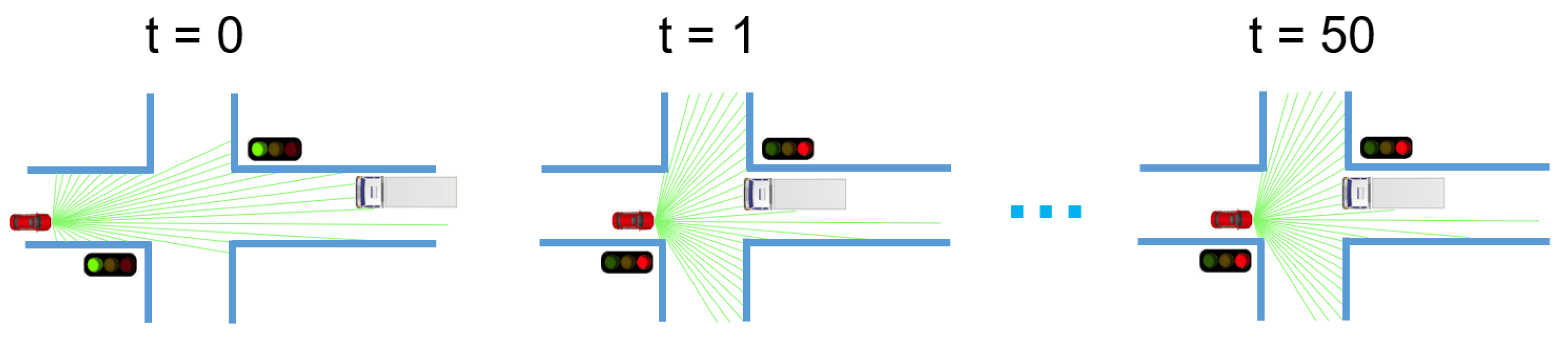
In this paper, we believe that both TAF and SAF are essential for moving objects identification, and only SAF is useful for LiDAR data enrichment. The later statement is easy to prove: consider a stationary LiDAR, because it is not moving, the strategy of combining multiple temporally adjacent frames will not add more valuable information to the current observation. Therefore, only SAF is useful for LiDAR data enrichment. To prove the first statement, please refer to Figure 3 for an illustrative example. In Figure 3, a SDV (Self-Driving Vehicle) equipped with a LiDAR is represented as a red vehicle. It observes an oncoming truck at time step . When the red light was on at time , both cars stopped at an intersection. The two cars continue to wait for the green light until the time . The wait may continue, depending on how long the red light is still on. For the SDV, if it wants to classify the oncoming truck as a moving object, then it has to compare the currently observed scan with the scan captured at . It suggests that the size of the TAF set should be larger than 50, which might be too large for practical usage. In contrast, if not only the TAF, but also the SAF is utilized, then a much smaller memory requirement is needed.
3.2. Moving Point Identification Based on Range Image Comparison
By comparing the current scan with its SAF and TAF, moving points can be identified. Similar to the work proposed in [9,18,23,24], we choose to use visibility-based method [11] for moving point identification. Compared with the voxel grid-based approach [25], the visibility-based method avoids the computationally expensive ray tracing operator, and by directly processing the point cloud, it also avoids the quantization error caused by the construction of the grid map.
For each LiDAR frame , its corresponding range image is firstly calculated using the approach of PBEA (Projection By Elevation Angle) proposed in [1]. To minimize the quantization error, the width and height of the range image are set to relatively large values.
For a point in the current frame , it is firstly transformed to the local coordinate system of any of its SAF or TAF by:
where represents the relative transformation between current frame c and its adjacent frame A. is then projected to the range image coordinate , where and are the column and row indexes of the range image respectively. The norm of is then compared with the value stored in the range image . The range difference is then calculated as:
where represents the range value stored at in the range image .
The value of is a strong indicator for moving point identification, and is widely used in the previous works [18,23]. In this paper, we make two modifications to this method:
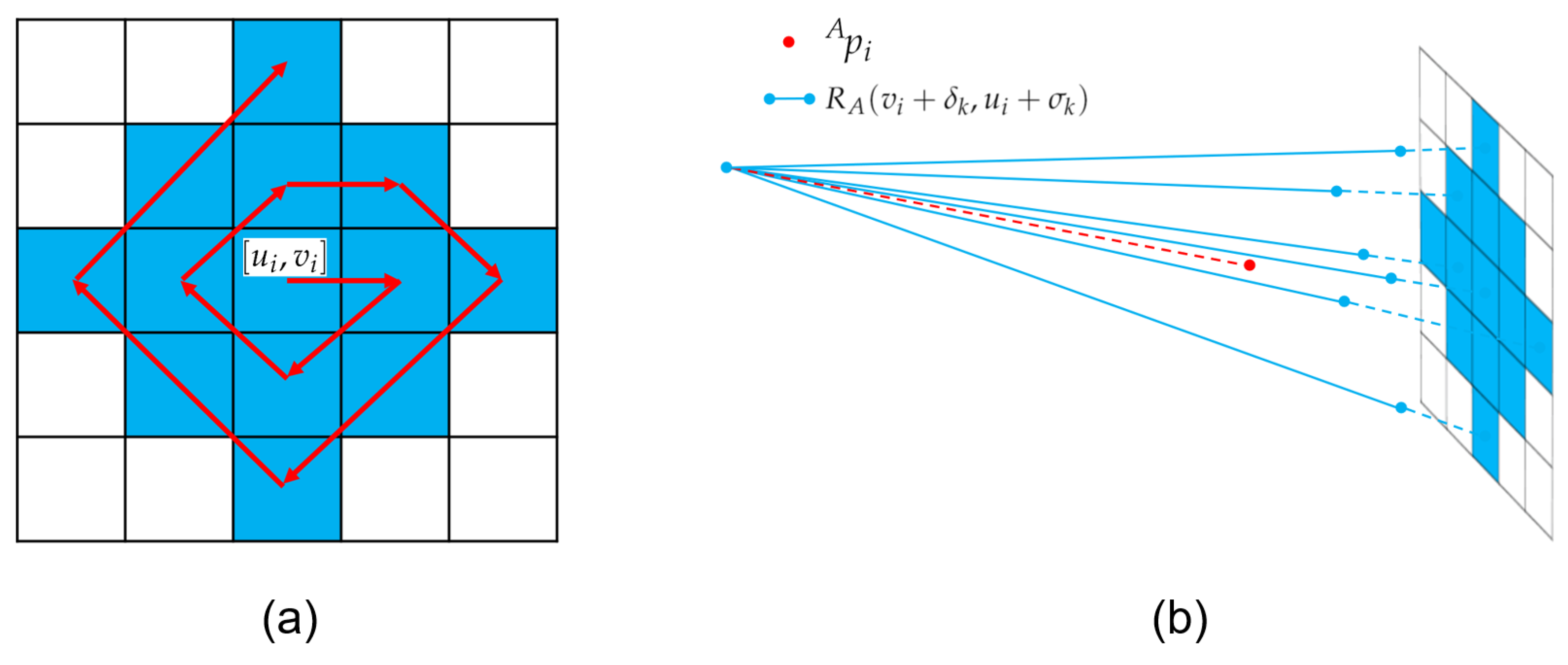
Firstly, in practice, the relative transformation between two frames may contain errors. In addition, the range image representation also contains quantization errors [1]. Taking these errors into account, should be compared not only with , but also with a small area around in the range image. Therefore, Equation (2) is modified to:
where , . The values of and represent the traversal order as shown in Figure 4a. The values of and are also shown in Figure 4b.
Secondly, in previous work, only the absolute value of was used as the moving indicator. In this paper, we argue that not only the absolute value, but also the sign of , contain valuable information for moving point identification. Based on the set of , five possible cases might occur:
- Case 1: There exist some in satisfying , where is a positive value.
- Case 2: All are less than .
- Case 3: All are greater than .
- Case 4: Some are greater than , whilst others are less than .
- Case 5: None of the values in are valid. This is caused by the blank area in the range image, which may be caused by the absorption of target objects, or an ignored uncertain range measurement [24].
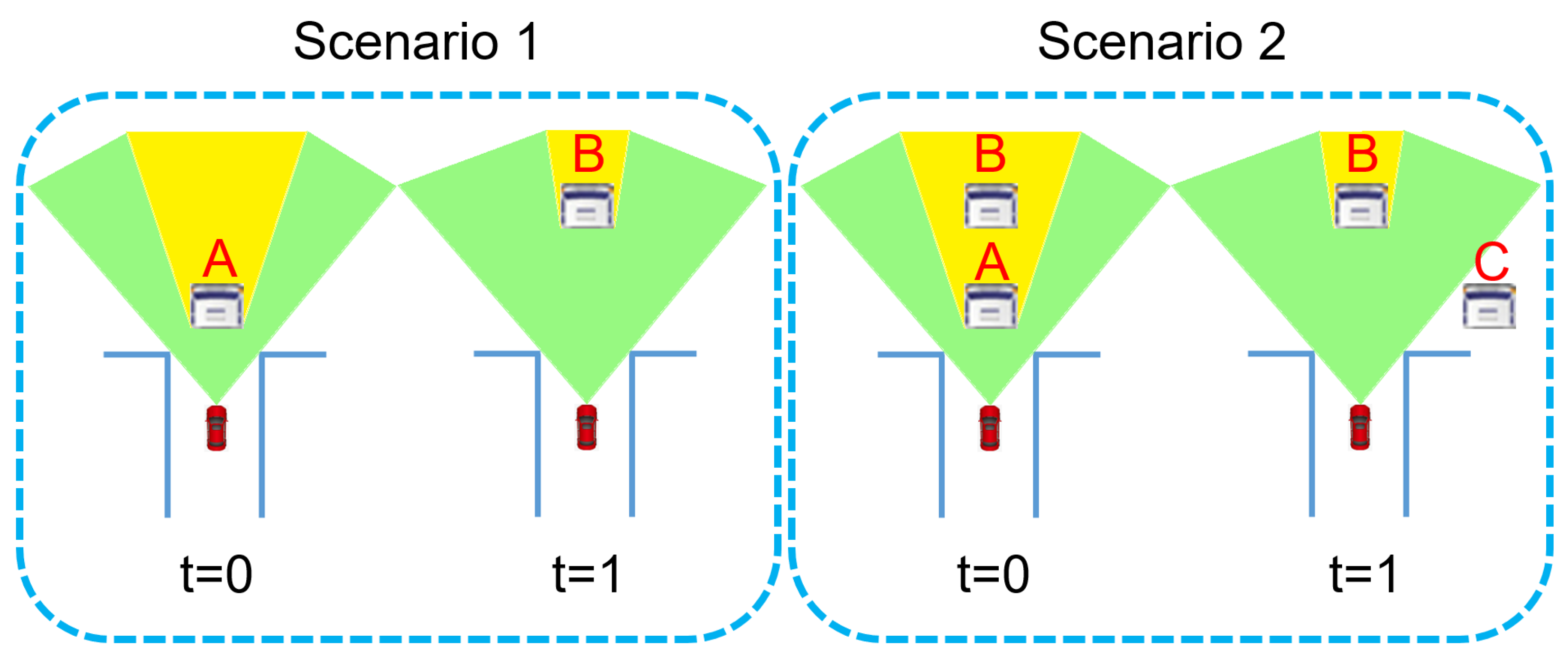
Among these five cases, Case 1 suggests that the query point is probably static, because a close-by point can be found in previous adjacent frames. Case 2 suggests that appears at a closer range than previously observed. This is a strong indicator for moving objects. Case 3 suggests that appears at a further range than previous observations. For this case, there are two possible explanations, as illustrated in Figure 5. In this illustrative example, consider a SDV (shown as the red car) observes an object at location A at time , and observes another object at location B at time . For position B, it is located in the occluded area at time and becomes observable at time . Therefore, it should be classified into Case 3. However, it cannot be judged whether object B is a moving object that moves from A (illustrated as Scenario 1 in Figure 5), or it is a static object that already exists at time (illustrated as Scenario 2 in Figure 5). Therefore, Case 3 is ambiguous for moving object identification.
For Case 4, it suggests that the current observed point can be interpolated from the previous observations. If we fit a local plane or calculate the point normal, then the point-to-plane distance [18] may be zero. Therefore, Case 4 is also not a good indicator for moving objects. In Case 5, the current observed point cannot find any correspondence in the previous observations. There is no motion evidence for this point, and the point remains as it is in the LiDAR enrichment procedure.
From the above analysis, we show that only Case 2 is a strong motion indicator. In practice, the current scan is separately compared with each frame in the SAF and TAF. Each comparison will classify the current point into one of the five cases. We then simply count the number of times that a point is classified into Case 2. If the count value is greater than a threshold, then this point is considered as a moving point. The moving points are then removed from the current scan for future frame enrichment.
3.3. LiDAR Data Enrichment Based on Spatial Adjacent Frames
To enrich the current scan, just as mentioned in Section 3.1, only frames in the SAF set are utilized. Note that for each frame in the SAF set, it has already gone through the moving point identification and exclusion procedure described in the previous subsection. All the remaining points in the SAF set are then transformed into the current frame coordinate, and compared with the current frame. Points that are classified as Case 1 or Case 3 are used to enrich the current frame. The reason for using the points belonging to Case 3 is that these probably static points (not classified as Case 2) are located in the occluded area of the current observation. Even if some of the points are misclassified, they have little impact on SDV planning or driving behavior.
It should be emphasized that in the previous subsection, the current scan is transformed into the previous frames’ coordinate for moving object identification, whilst in this subsection, the previous scans (with moving objects excluded) are transformed into the current frame coordinate to enrich the current scan. In these two scenarios, the functions of the reference coordinate system and the target coordinate system are opposite. It is possible that a point in the target frame is classified as Case 2 when compared with the reference frame, whilst its corresponding point in the reference frame is classified as Case 3 when it is compared with the target frame.
Bearing this in mind, when a new frame is added to the SAF set, it has already been compared with these existing frames in the SAF set. However, the frames that already exist in the SAF set have not yet been compared with this newly added frame. Therefore, these existing frames should also be compared with this newly added frame to find more moving points. These newly found moving points are also removed before their comparison to the current scan for possible LiDAR data enrichment. The whole algorithm is summarized in Algorithm 1.
| Algorithm 1 LiDAR data enrichment using SAF and TAF |
|
4. Experimental Results
4.1. Experimental Setup
We perform experiments on Semantic KITTI dataset [20]. This dataset not only provides semantic labels for each LiDAR point, but also a more accurate LiDAR pose for each LiDAR scan. These poses are obtained using the offline graph SLAM algorithm, and are more accurate than the poses provided in the original KITTI dataset [26]. For the experiments below, we directly use these ground-truth poses to assemble adjacent LiDAR frames together.
The main contribution of this paper is to enrich the LiDAR scan by fusing adjacent frames while simultaneously removing the “ghost” track caused by moving objects. Therefore, we first classify each point in the LiDAR frame as ground/non-ground. The ground points are then removed, and the following experiments are purely performed on non-ground points. Ground segmentation is generally considered to be an almost solved problem [27], especially in urban structured environment, where the roads are mostly flat. For ground segmentation, we use the method proposed in [13].
4.2. Experiments on Moving Point Identification
We first perform experiments on moving point identification. The reason why we prefer to use the term “moving point” rather than “moving object” is to emphasize that our method directly deals with LiDAR points, and we did not perform any object segmentation [28] or region growing technique as used in [18].
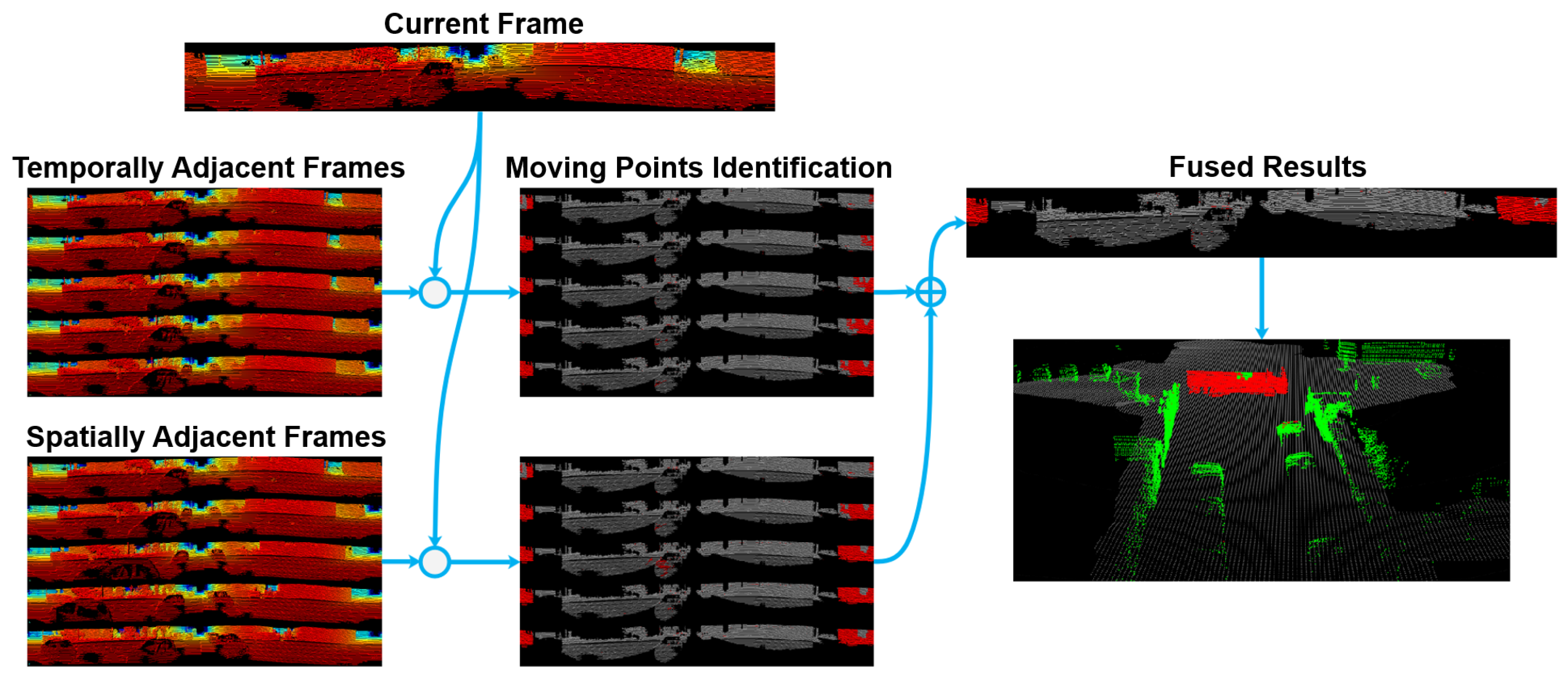
For moving point identification, a qualitative example is shown in Figure 6. The current frame is compared with each frame in the TAF set and SAF set respectively. Points that are classified as Case 2 are considered as potential moving points. From all the comparisons, the number of times that a point is classified as Case 2 is counted. If the count value is greater than a threshold, this point is classified as a moving point, which are colored as red in Figure 6.
By carefully examining the results in this example, we can observe that all the five results from the TAF set cannot classify the entire van as a moving object. In contrast, three of the five results in the SAF comparison successfully classified most of the van as moving points. This clearly shows that not only the TAF set, but also the SAF set are indispensable for moving point identification. The reason that some points in the top middle part of the van are not classified as dynamic is that these points correspond to the invalid areas in the previous observations, which are probably caused by too far-away observations. Therefore, these points are classified as belonging to Case 5.
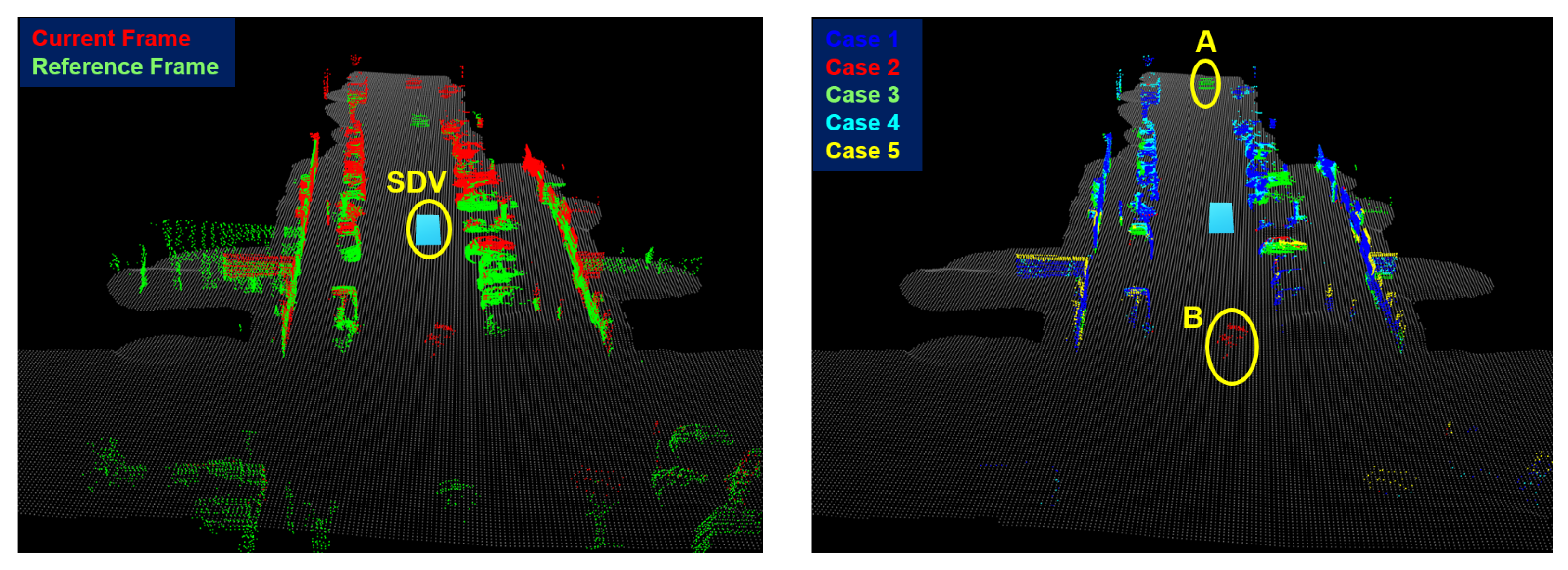
Another example of moving point identification is shown in Figure 7, where the current frame is compared with a reference frame stored in the SAF set. In this scenario, two vehicles, A and B, are moving in the same direction with the SDV. Vehicle A is in front of the SDV and B is behind. As shown in Figure 7, vehicle A is classified as Case 3, and vehicle B is classified as Case 2. In our implementation, only points belonging to Case 2 are considered as moving points. Although vehicle A is not judged as a moving object, it does not affect the data enrichment procedure. Since the previous observations of vehicle A are within the close range of the current observation, they are more likely to be classified as Case 2. Recall that only points classified as Case 1 or Case 3 are used to enrich the current scan, so failure to classify vehicle A will not affect the data enrichment step.
Using the free/occupancy/occlusion terminology in the occupancy grid mapping literature [29], vehicle A actually corresponds to the change from occlusion to occupancy (O2O) and vehicle B corresponds to the change from free to occupancy (F2O). These two situations are usually considered the same in the previous literature [18,19,30]. However, in this work, we emphasized the difference between these two situations, denoted as Case 2 and Case 3 respectively, and believed that F2O is more reliable motion evidence than O2O. If O2O is also considered as evidence of motion, then there will be too many false positives, as illustrated in Figure 7 (Case 3, colored as green).
4.3. Experiments on LiDAR Data Enrichment
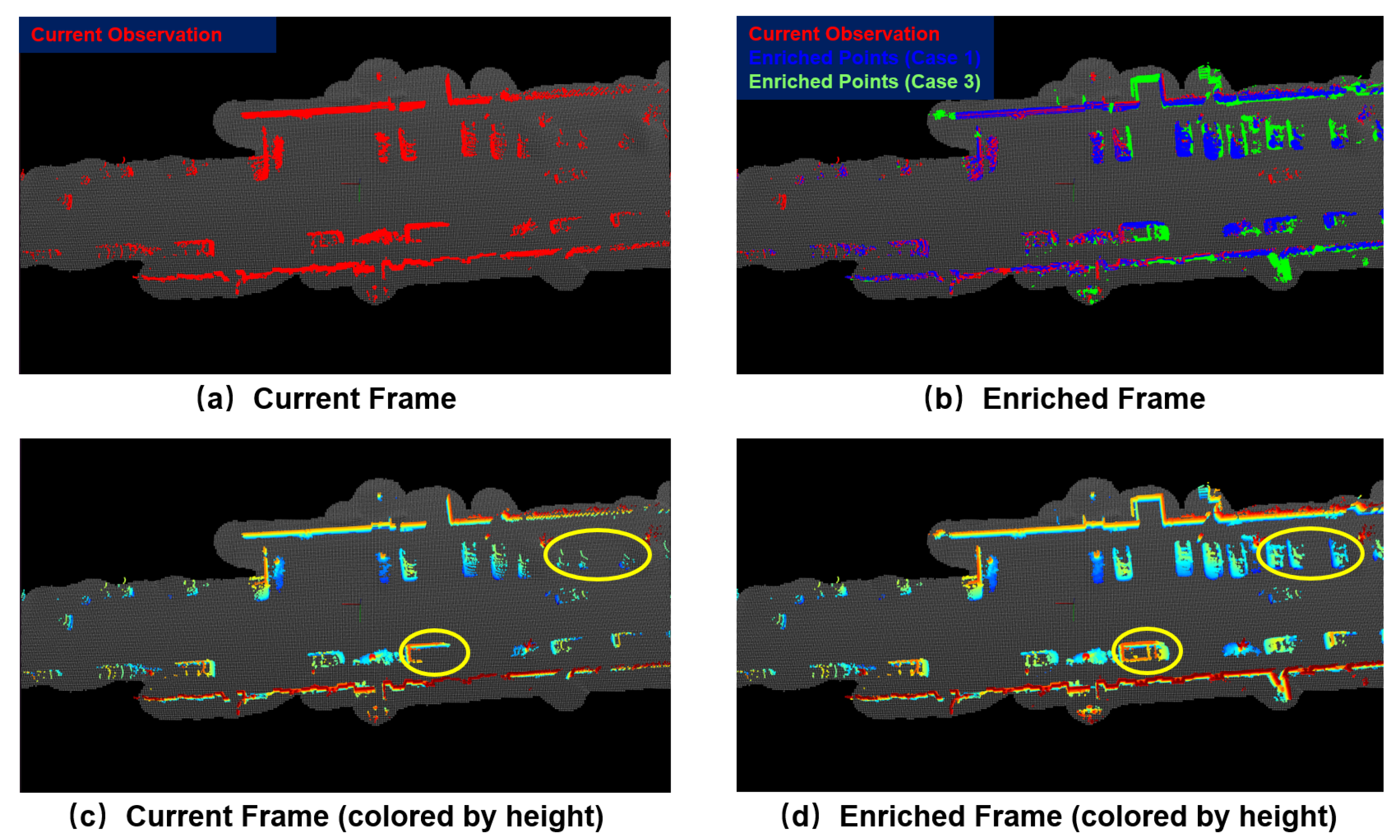
For each frame in the SAF set, its moving points are firstly removed. The remaining points are then transformed to the current frame coordinate, and compared with the current frame. Only points classified as Case 1 or Case 3 are used to enrich the current frame. An illustrative example is shown in Figure 8.
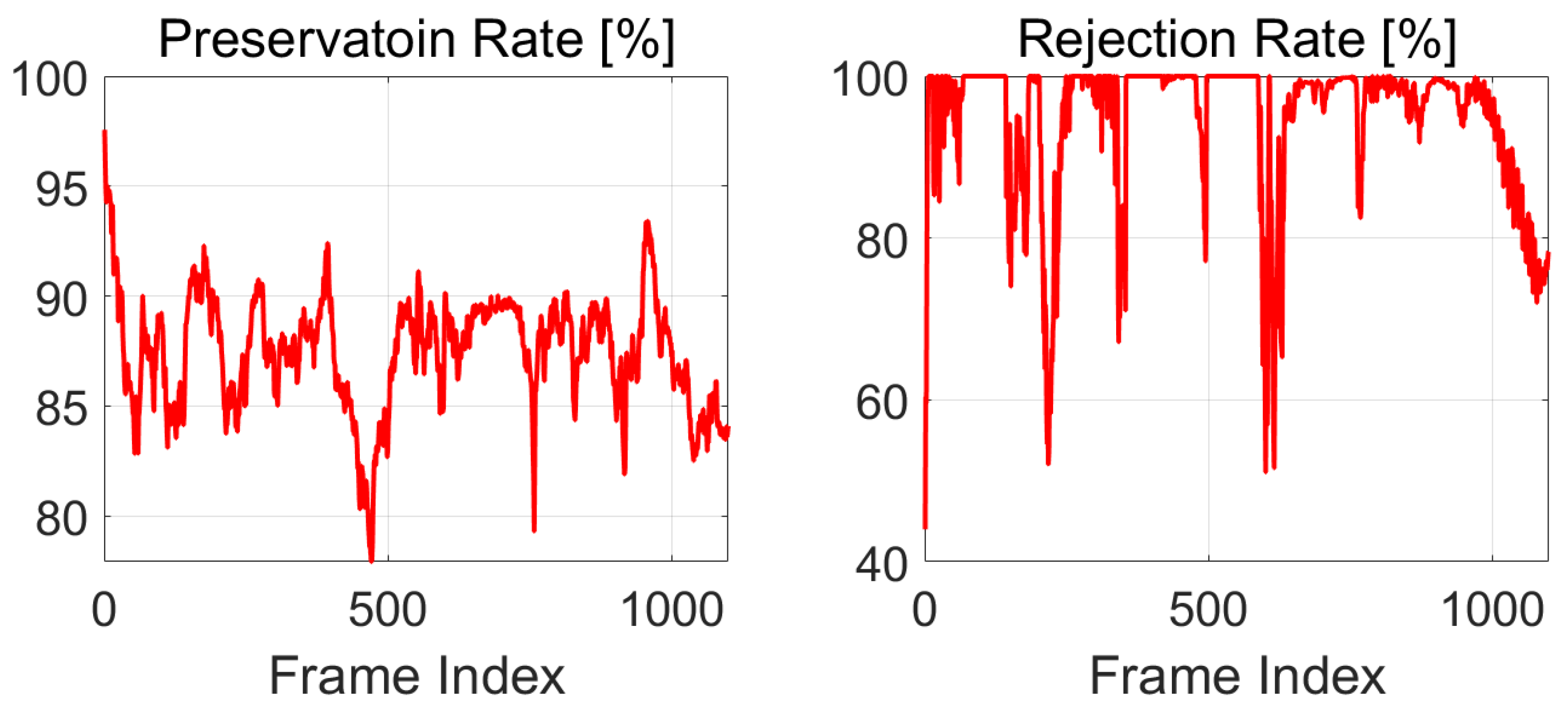
To quantitatively evaluate the LiDAR enrichment performance, we perform experiments on the whole SemanticKITTI sequence 07 dataset, which contains 1101 frames. For performance evaluation, we used two recently proposed performance indicators [11]: Preservation Rate (PR) and Rejection Rate (RR). Compared with the commonly used precision and recall rate, these two indicators are more sensitive to the removal of moving objects, and are more suitable for static map construction tasks.
Compared to the offline static map building scenario in [11], the method proposed in this paper is an online algorithm because we only use historical frames to enrich the current frame. Therefore, the PR and RR could be calculated for each single frame.
We use the moving object label provided in Semantic KITTI to generate ground-truth. For each frame, all the points labeled as static in its SAF set constitute the point set that should be enriched to the current frame, and the points labeled as moving objects constitute the point set that should be removed in the data enrichment procedure. Let and represent the static point set and dynamic point set respectively.
The preservation rate (PR)) is then defined as the ratio of the number of preserved static points to the number of points in . The rejection rate (RR) is defined as the ratio between the number of rejected moving points and the number of points in .
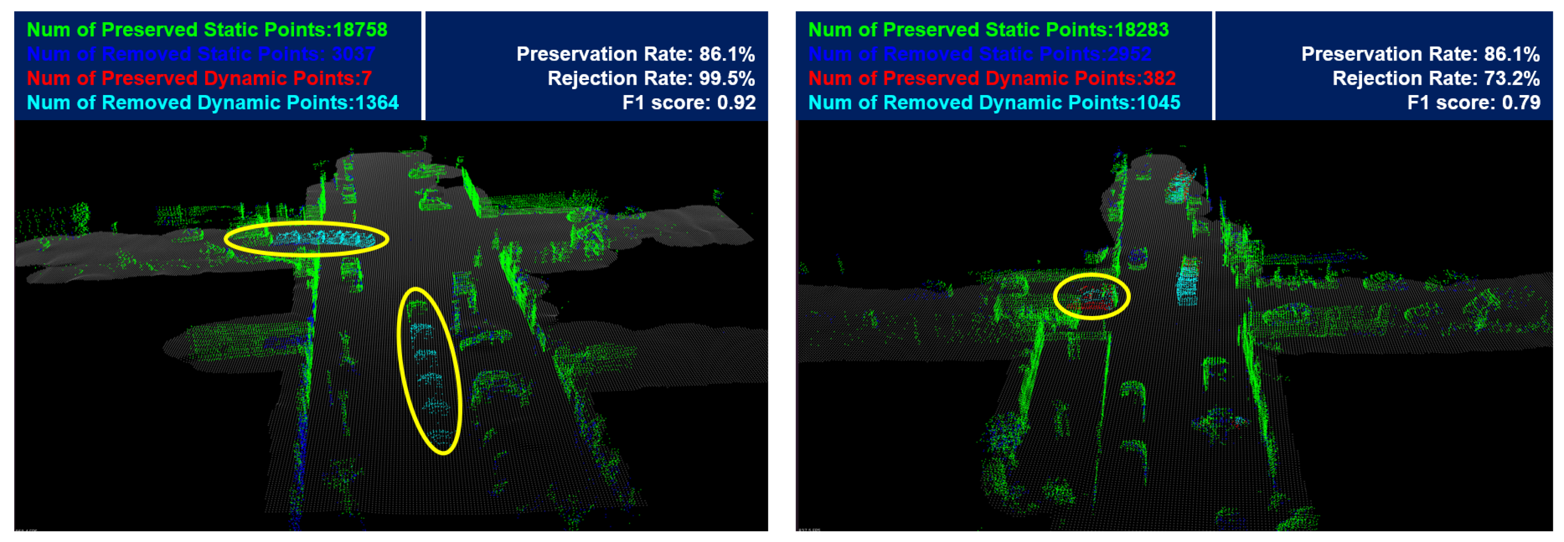
The PR and RR of all the 1100 frames (except the first frame) in SemanticKITTI Sequence 07 dataset are plotted in Figure 9. Two representative scenarios are shown in Figure 10. In Figure 10 left, two moving vehicles are correctly identified, and their “ghost” tracks are successfully removed, so the rejection rate is as high as 99.5%. For the scenario shown in Figure 10 right, the vehicle circled by the yellow ellipse has been parked for a period of time. Therefore, it is not correctly recognized as a moving object, and the rejection rate reduces to 73.2%. Regarding the preservation rate, it is approximately the same for both scenarios.
The computational speed of our method is also evaluated on the SemanticKITTI dataset. Except for the ground segmentation part, the average processing time of our entire algorithm is about 44.97 milliseconds per frame, with a standard deviation of 6.38 milliseconds. Therefore, it meets the real-time requirements of SDV (less than 100 milliseconds).
We also compared the performance of the proposed method with several state-of-the-art methods [9,25,31]. For these previous works, we directly use the results reported in [11]. In order to make a fair comparison with [11], we add the corresponding numbers (num of preserved static/dynamic points, num of total static/dynamic points) between 630th frame and 820th frame, and calculate the PR and RR based on the sum. The results are displayed in Table 1. It is observed that our method outperforms most previous methods [9,25,31], and performs on par with [11]. It should be emphasized that all these previous methods are designed as batch mode for offline usage. In contrast, our method is the only method that can run in real-time for online usage. This clearly distinguishes our approach from previous work. The reason that PR is a bit low is that only the points classified as Case 1 or Case 3 are preserved. The points belonging to Case 4 are removed. By carefully analyzing the points belonging to Case 4, PR may be improved without affecting RR performance. We leave this as future work.
5. Concluding Remarks
In this paper, we propose a novel LiDAR enrichment technique by using a multi-frame fusion strategy. We first proposed the concepts of spatially adjacent frames (SAF) and temporal adjacent frames (TAF). Then we show that both SAF and TAF are essential for moving point identification, and only SAF is useful for LiDAR data enrichment.
Experiments are performed on publicly available SemanticKITTI dataset, and compared with state-of-the-art approaches. Results show that the proposed method outperforms most previous methods, and performs on par with a recently proposed method [11]. Compared to these previous approaches, the proposed method is the only approach that can run in real-time for online usage.
Enriching the sparse LiDAR point cloud has many potential usages. Previous work has shown that the enriched point clouds can improve the performance of LiDAR odometry [8], object detection [32], or semantic segmentation [33]. However, most of these previous works adopt learning-based strategies and try to enrich LiDAR data from a single frame. In this paper, we emphasize that in the context of autonomous driving, each single frame is just a local snapshot of the environment. As LiDAR moves with the SDV, multiple snapshots can be obtained. If these local snapshots can be properly assembled, a dense representation of the environment can naturally be obtained. Therefore, we should not limit ourselves to processing a single frame, but should process multiple frames. Another advantage of processing multiple frames is that we can ensure the stability of the environment perception module, that is, the environment perception results should be consistent between consecutive frames. This stability or consistency is a key enabling factor for the stable and smooth control of SDV.
Author Contributions
Conceptualization, H.F.; methodology, H.F.; software, H.F. and H.X.; validation, X.H. and H.X.; formal analysis, H.F. and H.X.; investigation, H.F. and X.H.; resources, H.F.; data curation, H.F. and B.L.; writing—original draft preparation, H.F.; writing—review and editing, H.X., X.H., and B.L.; visualization, H.F.; All authors have read and agreed to the published version of the manuscript.
Funding
This research received no external funding.
Institutional Review Board Statement
Not applicable.
Informed Consent Statement
Not applicable.
Conflicts of Interest
The authors declare no conflict of interest.
References
- Wu, T.; Fu, H.; Liu, B.; Xue, H.; Ren, R.; Tu, Z. Detailed analysis on generating the range image for lidar point cloud processing. Electronics 2021, 10, 1224. [Google Scholar] [CrossRef]
- Bosse, M.; Zlot, R.; Flick, P. Zebedee Design of a Spring-Mounted 3-D Range. IEEE Trans. Robot. 2012, 28, 1–15. [Google Scholar] [CrossRef]
- Lin, J.; Zhang, F. Loam livox: A fast, robust, high-precision LiDAR odometry and mapping package for LiDARs of small FoV. In Proceedings of the 2020 IEEE International Conference on Robotics and Automation (ICRA), Paris, France, 31 May–31 August 2020. [Google Scholar]
- Uhrig, J.; Schneider, N.; Schneider, L.; Franke, U.; Brox, T.; Geiger, A. Sparsity invariant CNNs. In Proceedings of the International Conference on 3D Vision (3DV), Qingdao, China, 10–12 October 2017. [Google Scholar]
- Ku, J.; Harakeh, A.; Waslander, S.L. In Defense of Classical Image Processing: Fast Depth Completion on the CPU. In Proceedings of the 2018 15th Conference on Computer and Robot Vision (CRV), Toronto, ON, Canada, 8–10 May 2018; pp. 16–22. [Google Scholar] [CrossRef]
- Gu, J.; Xiang, Z.; Ye, Y.; Wang, L. DenseLiDAR: A Real-Time Pseudo Dense Depth Guided Depth Completion Network. IEEE Robot. Autom. Lett. 2021, 6, 1808–1815. [Google Scholar] [CrossRef]
- Shan, T.; Wang, J.; Chen, F.; Szenher, P.; Englot, B. Simulation-based Lidar Super-resolution for Ground Vehicles. Robot. Auton. Syst. 2020, 134, 103647. [Google Scholar] [CrossRef]
- Yue, J.; Wen, W.; Han, J.; Hsu, L.T. 3D Point Clouds Data Super Resolution Aided LiDAR Odometry for Vehicular Positioning in Urban Canyons. IEEE Trans. Veh. Technol. 2021, 70, 4098–4112. [Google Scholar] [CrossRef]
- Kim, G.; Kim, A. Remove, then Revert: Static Point cloud Map Construction using Multiresolution Range Images. In Proceedings of the International Conference on Intelligent Robots and Systems (IROS), Las Vegas, NV, USA, 24 October–24 January 2020. [Google Scholar] [CrossRef]
- Pagad, S.; Agarwal, D.; Narayanan, S.; Rangan, K.; Kim, H.; Yalla, G. Robust Method for Removing Dynamic Objects from Point Clouds. In Proceedings of the IEEE International Conference on Robotics and Automation, Paris, France, 31 May–30 June 2020; pp. 10765–10771. [Google Scholar] [CrossRef]
- Lim, H.; Hwang, S.; Myung, H. ERASOR: Egocentric Ratio of Pseudo Occupancy-Based Dynamic Object Removal for Static 3D Point Cloud Map Building. IEEE Robot. Autom. Lett. 2021, 6, 2272–2279. [Google Scholar] [CrossRef]
- Mur-Artal, R.; Montiel, J.M.; Tardos, J.D. ORB-SLAM: A Versatile and Accurate Monocular SLAM System. IEEE Trans. Robot. 2015, 31, 1147–1163. [Google Scholar] [CrossRef] [Green Version]
- Xue, H.; Fu, H.; Ruike, R.; Jintao, Z.; Bokai, L.; Yiming, F.; Bin, D. LiDAR-based Drivable Region Detection for Autonomous Driving. In Proceedings of the International Conference on Intelligent Robots and Systems (IROS), Prague, Czech Republic, 1 March 2021. [Google Scholar]
- Yang, Q.; Yang, R.; Davis, J.; Nist, D. Spatial-Depth Super Resolution for Range Images. In Proceedings of the 2007 IEEE Conference on Computer Vision and Pattern Recognition, Minneapolis, MN, USA, 17–22 June 2007. [Google Scholar]
- Chen, Y.; Yang, B.; Liang, M.; Urtasun, R. Learning joint 2D-3D representations for depth completion. In Proceedings of the IEEE International Conference on Computer Vision, Seoul, Korea, 27 October–3 November 2019; pp. 10022–10031. [Google Scholar] [CrossRef]
- Badino, H.; Huber, D.; Park, Y.; Kanade, T. Fast and accurate computation of surface normals from range images. In Proceedings of the IEEE International Conference on Robotics and Automation, Shanghai, China, 9–13 May 2011; pp. 3084–3091. [Google Scholar] [CrossRef]
- Zhao, Y.; Bai, L.; Zhang, Z.; Huang, X. A Surface Geometry Model for LiDAR Depth Completion. IEEE Robot. Autom. Lett. 2021, 6, 4457–4464. [Google Scholar] [CrossRef]
- Yoon, D.; Tang, T.; Barfoot, T. Mapless online detection of dynamic objects in 3D lidar. In Proceedings of the 2019 16th Conference on Computer and Robot Vision, CRV, Kingston, QC, Canad, 29–31 May 2019; pp. 113–120. [Google Scholar] [CrossRef] [Green Version]
- Chen, X.; Li, S.; Mersch, B.; Wiesmann, L.; Gall, J.; Behley, J.; Stachniss, C. Moving Object Segmentation in 3D LiDAR Data: A Learning-based Approach Exploiting Sequential Data. IEEE Robot. Autom. Lett. 2021, 1–8. [Google Scholar] [CrossRef]
- Behley, J.; Garbade, M.; Milioto, A.; Behnke, S.; Stachniss, C.; Gall, J.; Quenzel, J. SemanticKITTI: A dataset for semantic scene understanding of LiDAR sequences. In Proceedings of the IEEE/CVF International Conference on Computer Vision, ICCV, Seoul, Korea, 27 October–3 November 2019. [Google Scholar]
- Luo, W.; Yang, B.; Urtasun, R. Fast and Furious: Real Time End-to-End 3D Detection, Tracking and Motion Forecasting with a Single Convolutional Net. In Proceedings of the IEEE Computer Society Conference on Computer Vision and Pattern Recognition, Salt Lake, UT, USA, 18–22 June 2018; pp. 3569–3577. [Google Scholar] [CrossRef]
- Zhang, J.; Singh, S. LOAM: Lidar Odometry and Mapping in Real-time. In Robotics: Science and Systems; 2014; pp. 1–8. Available online: https://www.ri.cmu.edu/pub_files/2014/7/Ji_LidarMapping_RSS2014_v8.pdf (accessed on 8 September 2021).
- Pomerleau, F.; Krüsi, P.; Colas, F.; Furgale, P.; Siegwart, R. Long-term 3D map maintenance in dynamic environments. In Proceedings of the IEEE International Conference on Robotics and Automation, Hong Kong, China, 31 May–7 June 2014; pp. 3712–3719. [Google Scholar] [CrossRef] [Green Version]
- Fu, H.; Xue, H.; Ren, R. Fast Implementation of 3D Occupancy Grid for Autonomous Driving. In Proceedings of the 2020 12th International Conference on Intelligent Human-Machine Systems and Cybernetics, IHMSC 2020, Hangzhou, China, 22–23 August 2020; Volume 2, pp. 217–220. [Google Scholar] [CrossRef]
- Wurm, K.M.; Hornung, A.; Bennewitz, M.; Stachniss, C.; Burgard, W. OctoMap: A Probabilistic, Flexible, and Compact 3D Map Representation for Robotic Systems. In Proceedings of the International Conference on Robotics and Automation (ICRA), Anchorage, Alaska, 3–8 May 2010. [Google Scholar]
- Geiger, A.; Lenz, P.; Stiller, C.; Urtasun, R. Vision meets Robotics: The KITTI Dataset. Int. J. Robot. Res. 2013, 32, 1231–1237. [Google Scholar] [CrossRef] [Green Version]
- Jiang, C.; Paudel, D.P.; Fofi, D.; Fougerolle, Y.; Demonceaux, C. Moving Object Detection by 3D Flow Field Analysis. IEEE Trans. Intell. Transp. Syst. 2021, 22, 1950–1963. [Google Scholar] [CrossRef]
- Zermas, D.; Izzat, I.; Papanikolopoulos, N. Fast segmentation of 3D point clouds: A paradigm on LiDAR data for autonomous vehicle applications. In Proceedings of the IEEE International Conference on Robotics and Automation, Singapore, 29 May–3 June 2017; pp. 5067–5073. [Google Scholar] [CrossRef]
- Thrun, S. Learning Occupancy Grid Maps With Forward Sensor Models. Auton. Robot. 2003, 15, 111–127. [Google Scholar] [CrossRef]
- Petrovskaya, A.; Thrun, S. Model based vehicle tracking for autonomous driving in urban environments. Robot. Sci. Syst. 2009, 4, 175–182. [Google Scholar] [CrossRef]
- Schauer, J.; Nuchter, A. The Peopleremover-Removing Dynamic Objects from 3-D Point Cloud Data by Traversing a Voxel Occupancy Grid. IEEE Robot. Autom. Lett. 2018, 3, 1679–1686. [Google Scholar] [CrossRef]
- Wirges, S.; Yang, Y.; Richter, S.; Hu, H.; Stiller, C. Learned Enrichment of Top-View Grid Maps Improves Object Detection. In Proceedings of the 2020 IEEE 23rd International Conference on Intelligent Transportation Systems, ITSC 2020, Rhodes, Greece, 20–23 September 2020. [Google Scholar] [CrossRef]
- Rist, C.; Emmerichs, D.; Enzweiler, M.; Gavrila, D. Semantic Scene Completion using Local Deep Implicit Functions on LiDAR Data. IEEE Trans. Pattern Anal. Mach. Intell. 2021, 1–19. [Google Scholar] [CrossRef] [PubMed]
Figure 1.
The current LiDAR frame (shown in (a)) only contains 28,894 non-ground points that are considered sparse. By assembling consecutive frames together, a denser representation can be obtained, as shown in (b). However, moving objects (highlighted as red points in (c)) leave “ghost” tracks in the assembled frame. Using the method proposed in this paper, these “ghost” tracks are successfully removed while the static environment is safely enriched, as shown in (d). The method proposed in [13] is utilized for ground/non-ground classification. The estimated ground surface is shown as gray points, while non-ground points are colored by height.
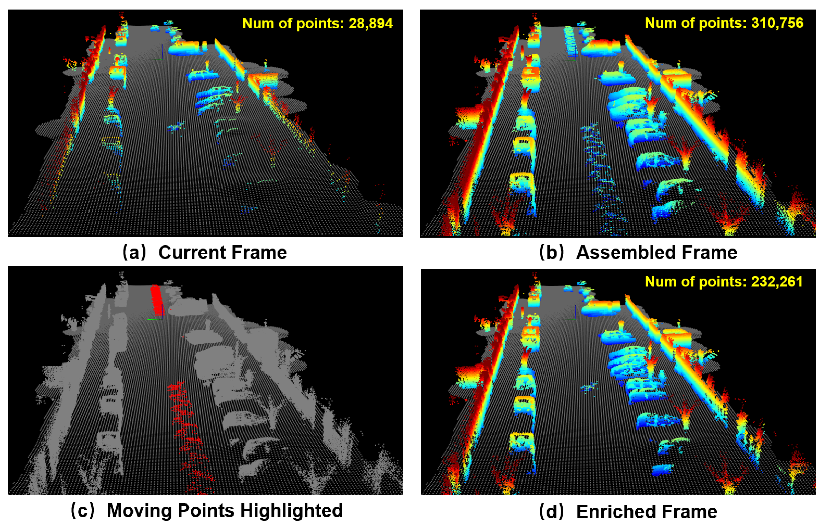
Figure 2.
For the current frame , its temporal adjacent frames is defined as the collection of frames that are temporal close to the current frame. Its spatial adjacent frame is defined as the frames that is spatially close to the current frame, and the distance between any two frames is greater than a distance threshold , i.e., .
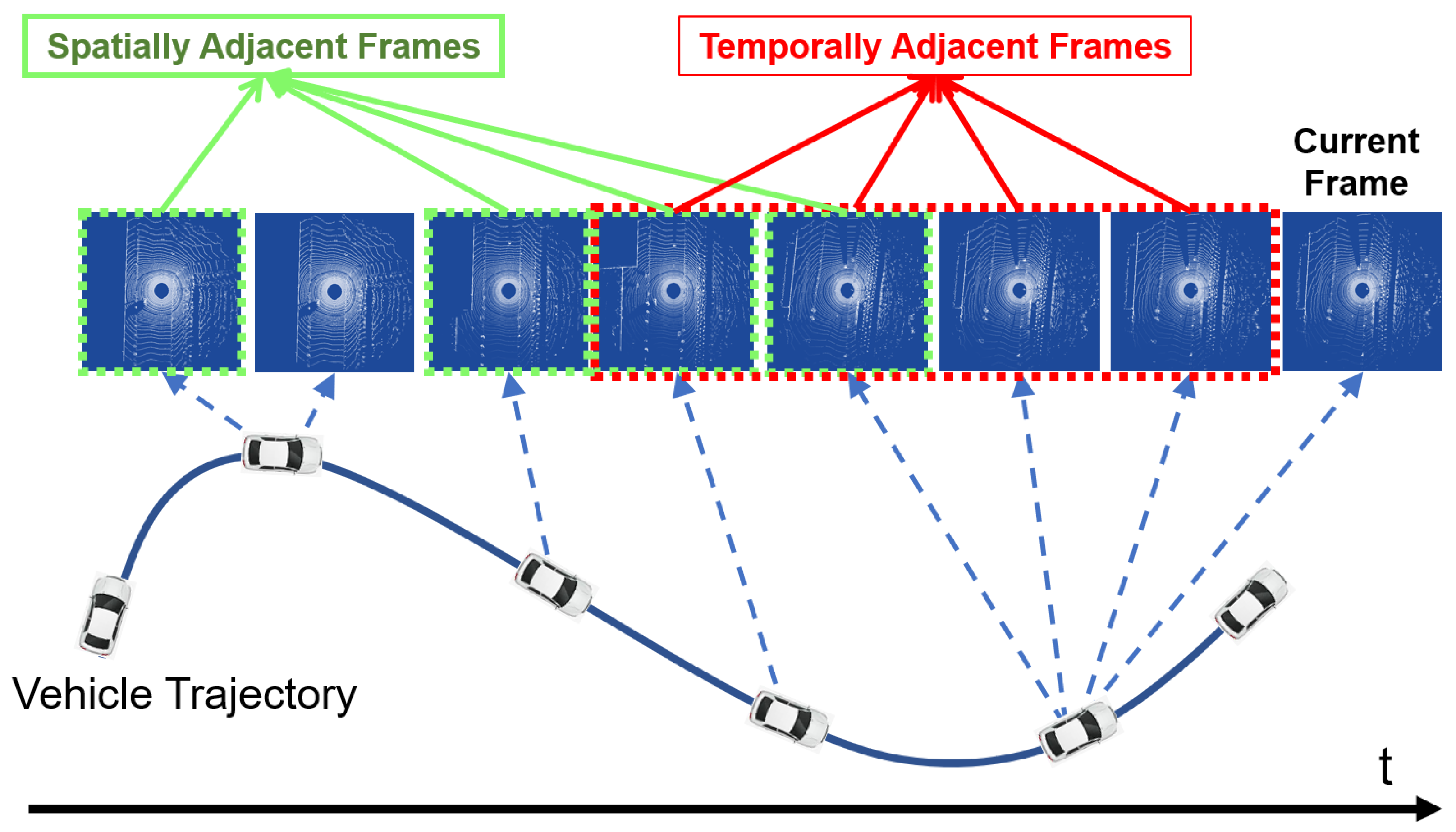
Figure 3.
An illustrative example showing a SDV (red car) equipped with LiDAR observing an oncoming truck at time . The two cars stopped at an intersection and wait for the green light from to .
Figure 3.
An illustrative example showing a SDV (red car) equipped with LiDAR observing an oncoming truck at time . The two cars stopped at an intersection and wait for the green light from to .

Figure 4.
Due to relative pose error and the range image quantization error, the current observed point should not merely be compared with , but also a small area around in the range image. Subfigure (a) shows the comparing order between the current observed point and the small area in the reference frame, while subfigure (b) shows an illustrative example.

Figure 5.
Two possible explanations for Case 3. In Scenario 1, the object in front of the SDV (shown as the red car) is indeed a moving object that moves from A () to B (). In Scenario 2, the object ahead moves from A () to C (), and the object at location B is a stationary object.
Figure 5.
Two possible explanations for Case 3. In Scenario 1, the object in front of the SDV (shown as the red car) is indeed a moving object that moves from A () to B (). In Scenario 2, the object ahead moves from A () to C (), and the object at location B is a stationary object.

Figure 6.
The current frame is compared with each of the five frames in the TAF set and SAF set, respectively. Points that are classified as Case 2 are considered as potential moving points. The 10 comparison results are then fused using a simple counting mechanism.
Figure 6.
The current frame is compared with each of the five frames in the TAF set and SAF set, respectively. Points that are classified as Case 2 are considered as potential moving points. The 10 comparison results are then fused using a simple counting mechanism.

Figure 7.
The image on the left shows the superposition of the current frame and reference frame (a frame in the SAF set). The image on the right shows the classification result obtained by comparing the current frame with the reference frame. It can be seen that the moving vehicle A in front of the SDV is classified as Case 3, and the vehicle B behind the SDV is classified as Case 2.

Figure 8.
The current observed points, the enriched points classified as Case 1 or Case 3 are colored with red, blue, and green, respectively, in (a,b). For the four vehicles enclosed by the yellow ellipse, they are difficult to identify in (c) due to the sparse observations from a single LiDAR frame. In contrast, from the enriched frame shown in (d), these four vehicles are easily recognized.

Figure 9.
The preservation rate and rejection rate calculated for each of the 1100 frames in Semantic KITTI sequence 07 dataset.
Figure 9.
The preservation rate and rejection rate calculated for each of the 1100 frames in Semantic KITTI sequence 07 dataset.

Figure 10.
The two moving vehicles (outlined by the yellow ellipse) shown in the left figure have been correctly identified as moving objects. Therefore, the rejection rate is as high as 99.5%. The vehicle shown in the right figure has not been identified as moving object, hence results in a low rejection rate of 73.2%.


Publisher’s Note: MDPI stays neutral with regard to jurisdictional claims in published maps and institutional affiliations. |
© 2021 by the authors. Licensee MDPI, Basel, Switzerland. This article is an open access article distributed under the terms and conditions of the Creative Commons Attribution (CC BY) license (https://creativecommons.org/licenses/by/4.0/).
Share and Cite
MDPI and ACS Style
Fu, H.; Xue, H.; Hu, X.; Liu, B. LiDAR Data Enrichment by Fusing Spatial and Temporal Adjacent Frames. Remote Sens. 2021, 13, 3640. https://0-doi-org.brum.beds.ac.uk/10.3390/rs13183640
AMA Style
Fu H, Xue H, Hu X, Liu B. LiDAR Data Enrichment by Fusing Spatial and Temporal Adjacent Frames. Remote Sensing. 2021; 13(18):3640. https://0-doi-org.brum.beds.ac.uk/10.3390/rs13183640
Chicago/Turabian StyleFu, Hao, Hanzhang Xue, Xiaochang Hu, and Bokai Liu. 2021. "LiDAR Data Enrichment by Fusing Spatial and Temporal Adjacent Frames" Remote Sensing 13, no. 18: 3640. https://0-doi-org.brum.beds.ac.uk/10.3390/rs13183640
Note that from the first issue of 2016, this journal uses article numbers instead of page numbers. See further details here.