
LiDAR-Based SLAM under Semantic Constraints in Dynamic Environments

1
Institute of Geospatial Information, PLA Strategic Support Force Information Engineering University, Zhengzhou 450052, China
2
Beijing Institute of Remote Sensing Information, Beijing 100011, China
3
Aviation University Air Force, Changchun 130012, China
*
Author to whom correspondence should be addressed.
Remote Sens. 2021, 13(18), 3651; https://0-doi-org.brum.beds.ac.uk/10.3390/rs13183651
Submission received: 20 July 2021
/
Revised: 25 August 2021
/
Accepted: 1 September 2021
/
Published: 13 September 2021
(This article belongs to the Special Issue Advances in Deep Learning Based 3D Scene Understanding from LiDAR)
Abstract
:Facing the realistic demands of the application environment of robots, the application of simultaneous localisation and mapping (SLAM) has gradually moved from static environments to complex dynamic environments, while traditional SLAM methods usually result in pose estimation deviations caused by errors in data association due to the interference of dynamic elements in the environment. This problem is effectively solved in the present study by proposing a SLAM approach based on light detection and ranging (LiDAR) under semantic constraints in dynamic environments. Four main modules are used for the projection of point cloud data, semantic segmentation, dynamic element screening, and semantic map construction. A LiDAR point cloud semantic segmentation network SANet based on a spatial attention mechanism is proposed, which significantly improves the real-time performance and accuracy of point cloud semantic segmentation. A dynamic element selection algorithm is designed and used with prior knowledge to significantly reduce the pose estimation deviations caused by SLAM dynamic elements. The results of experiments conducted on the public datasets SemanticKITTI, KITTI, and SemanticPOSS show that the accuracy and robustness of the proposed approach are significantly improved.
1. Introduction
With the development of technologies such as artificial intelligence (AI), 5G, and the Internet of Things (IoT), the coexistence and symbiosis between people and intelligent robots have quietly emerged. In monotonous, repetitive, dangerous, and unknown environments, intelligent robots have advantages over humans. The prerequisite for an intelligent robot to efficiently perform a given task is an accurate “understanding” of environments and expected impacts. Such understanding involves addressing a series of theoretical and technical issues for intelligent machines, such as environmental perception, environmental modelling, spatial reasoning, and calculations. This understanding is the key generic technology of the new generation of AI [1] and a new problem in surveying and mapping in the AI era [2]. Simultaneous localisation and mapping (SLAM) is a key technology for environmental detection and perception of intelligent robots, but despite significant progress over the past decade, most current mainstream SLAM algorithms operate stably only in static environments. The real world is dynamically changing, including both short-term changes, such as moving cars and pedestrians, and long-term changes, such as those in the environment caused by the change of seasons or the change from day to night. This dynamically changing environment poses new challenges to different modules of SLAM, e.g., pose estimation, feature extraction and tracking, and map construction. Currently, the principle of solving SLAM problems in a dynamic environment is to identify, track and process dynamic elements. Early studies focused on feature detection methods, but these methods are difficult to handle with slow- or fast-moving objects. With the rapid development of fully convolutional neural networks (FCNs), semantic information has been gradually included in the study of SLAM. Semantic segmentation results can reveal potential moving objects in the environment, which can help SLAM filter out moving objects in the feature tracking and mapping module to obtain more accurate pose estimation results. Some achievements have been made in the development of these methods; however, further optimisation is still needed.
According to the sensors used, SLAM can be either visual SLAM or light detection and ranging (LiDAR)-based SLAM. There are many types of visual sensors with low prices, and the research on image feature extraction and recognition and semantic segmentation has promoted the rapid development of visual SLAM, especially in the fields of semantic SLAM and SLAM in dynamic environments. LiDAR is currently used in many fields, including robotics, mobile mapping, autopilot, and three-dimensional (3D) reconstruction. In the research on LiDAR-based SLAM, a system framework based on an occupancy grid map has been established. However, compared with visual SLAM, the research on LiDAR-based SLAM mostly focusses on the direct processing of raw point cloud data collected in real time, while research on integrated object recognition, semantic segmentation and map construction still needs to be deepened.
A LiDAR-based SLAM under semantic constraints in dynamic environments is proposed in this study. Within the proposed approach, a spatial attention network (SANet) is used to achieve semantic segmentation of point clouds, and prior knowledge is used as guidance to establish environmental element classification criteria in order to pre-process the semantic segmentation results. Then, the dynamic elements in the environment are determined based on the environmental context information. Finally, pose estimation and semantic map construction are realised. The main contributions of this study are given below.
(1) A semantic segmentation method SANet is proposed for LiDAR point clouds based on a spatial attention mechanism and effectively improves the real-time performance and accuracy of semantic segmentation.
(2) A dynamic object screening strategy is proposed that can accurately filter moving objects in the environment and provide a reference for efficient and robust pose estimation.
(3) The performance of the proposed approach in a dynamic environment is evaluated for the KITTI and SemanticPOSS datasets. The experiments demonstrate that the proposed approach effectively improves the accuracy of pose estimation and has good performance.
The Section 1 is introduction. The rest of this paper is organised as follows. Section 2 presents a review of related work. Section 3 provides the details of our method. The experimental results for the SemanticKITTI, KITTI, and SemanticPOSS public datasets are presented in Section 4. Finally, a brief conclusion and discussion are presented in Section 5.
2. Related Work
2.1. Point Cloud Semantic Segmentation
The main data form used by LiDAR is point cloud data. How to extract valuable feature information from a large amount of point cloud data is always the focus of researchers. Point cloud semantic segmentation refers to the semantic information annotation on disordered and irregular point cloud data. In early studies, point cloud semantic annotation usually uses methods such as support vector machines (SVMs), conditional random field (CRF) and random forest (RF). For these methods, the semantic annotation categories are limited, and the accuracy is low, so they are not the mainstream methods at present. With a strong learning ability at the feature level, deep learning has gradually become the mainstream method for point cloud semantic segmentation. Different from the one-dimensional (1D) and two-dimensional (2D) data recognition fields (such as speech recognition and image recognition) that have been dominated by deep learning, the disorder and irregularity of point cloud data have limited the use of deep learning for these problems.
To solve the problem of semantic segmentation of 3D point cloud data, three types of deep learning methods have been roughly formed, i.e., point-based methods, image-based methods, and voxel-based methods [3]. The point-based methods use points as the input data of the CNNs, where the difficulty lies in how to extract the feature information of the points. A common solution is to extract local feature information through the neighbour point set for convolution operations. PointNet++ is one of the representative methods, which uses the multiscale domain information of points to extract local feature information for semantic segmentation. Subsequently, a variety of local feature extraction methods based on defining multiple neighbourhoods have emerged [4]. PointCNN is another representative method in which the spatial distance is used to determine the neighbourhood point set to extract local feature information for convolution operations [5]. The image-based methods originate from the excellent performance of deep learning in image recognition and semantic image segmentation. This type of method reduces the dimensionality of the 3D point cloud data by forming a 2D image in a specific manner and then projects the segmentation results back to the 3D data after semantic image segmentation. Common dimensionality reduction methods include multi-view segmentation and spherical projection. Multi-view segmentation collects images from various angles of the point cloud data and restores the 3D data in a multi-view form [6]. Representative spherical projection methods are SqueezeSeg [7,8,9] and RangeNet++ [10], with an accuracy (mean intersection-over-union (mIoU)) of approximately 53%. The voxel-based methods rasterise the point cloud and perform the convolution operation in the form of voxels, to reduce the impact due to the irregularity of point cloud data. The representative works, 3DCNN-DQN-RNN [11] and VolMap [12], are subject to the choice of voxel size. At present, the voxel-based method is effective for data with similar sizes; however, the objective phenomenon of “near big, far small” is a difficult problem for voxel-based methods to overcome.
2.2. Semantic SLAM
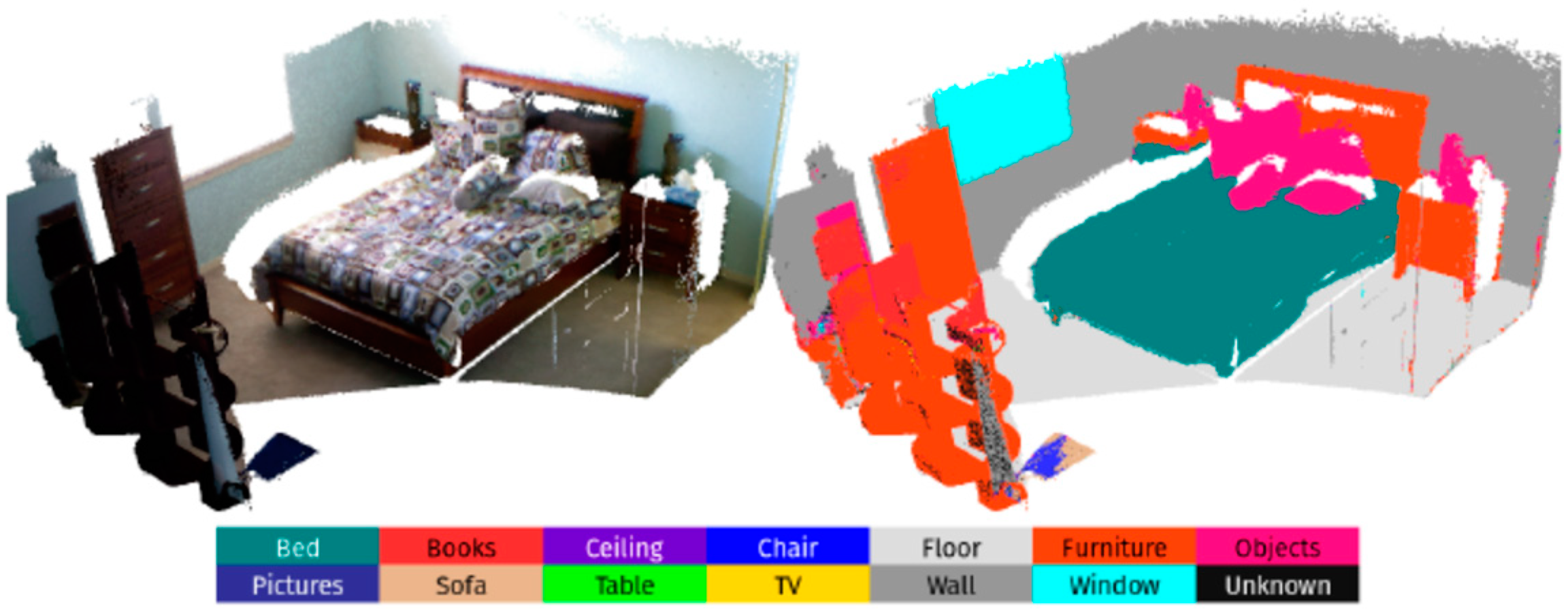
Semantic information is considered to be important information for robots to move from perceptual intelligence to cognitive intelligence. Semantic SLAM is an important way to integrate semantic information into environmental representation. In a review, Cadena et al. [13] summarised the research on semantic SLAM into two parts, i.e., semantic information to improve the accuracy of pose estimation and closed-loop detection, and the classification and mapping of environmental elements using SLAM to help robots deeply understand the environment. In recent studies on semantics-assisted SLAM, continuous pose estimation [14], scene object recognition [15,16], and global localisation [17] has been achieved based on Red, Green, Blue-Depth (RGB-D) sensors and semantic segmentation networks, and scene reconstruction has been achieved based on monocular camera and LiDAR [18]. Research on semantic-assisted SLAM focuses on environmental representation. Environmental elements are represented according to semantic concepts, and semantic maps, which classify and grade the elements, fall into two main categories, i.e., object-based semantic maps (Figure 1) and region-based semantic maps (Figure 2). An object-based semantic map accurately marks the objects in the scene on the map using technical methods, such as scene recognition and image segmentation. Early studies mainly used machine learning methods. Limketkai et al. [19] used a relational Markov network to perform semantic annotation on objects with obvious line features in the scene (such as walls, doors, and windows). In 2008, Andreas proposed the concept of a semantic map to analyse and mark the floor, ceiling, and wall using the characteristics of the indoor building structures based on the constructed 3D point cloud of the scene [20]. Since 2012, through CRF, Sengupta et al. [21,22,23] gradually realised the construction of a semantic map in outdoor environments in different expression forms, such as the Mesh form and the octree form, using visual sensors. With the development and popularisation of deep learning, the use of fully convolutional networks (FCNs) for semantic segmentation proposed in 2014 [24] became the basis of many studies. Based on FCNs, the accuracy of semantic segmentation has been further improved in many studies by increasing the number of convolution layers or adjusting the network structure, e.g., DeepLab [25], ICNet [26], and SegNet [27]. Although the accuracy of semantic segmentation has been improved, the methods that only use FCNs to achieve semantic segmentation still contain unclear descriptions of object contours and inaccurate edge information.
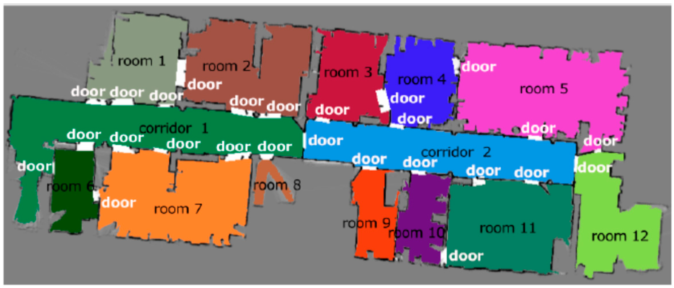
A region-based semantic map performs semantic annotation on each region in the scene, similar to the configuration of the “place name”. The initial research is based on the understanding of “door”, and different regions are usually separated by doors. Based on this understanding, Vasudevan et al. [28,29] applied a probabilistic approach to identify and annotate doors and specific objects and used simple spatial relations to strengthen the reasoning and annotation of specific regions. Rituerto et al. [30] further realised semantic annotation for doors, stairs and elevators. Liu et al. [31] used the semi-supervised clustering approach of the Markov process model to annotate the indoor environment and tried to use different clustering methods for semantic annotation [32,33,34]. In 2011, Pronobis et al. [35] proposed the multi-modal place classification system. A low-level classifier was used to identify the shape and size of the room and the objects, and then the room type was determined by reasoning through Markov chain. Pronobis et al. [36] continued and perfected the work in Ref. [35], and established a semantic annotation module for indoor environments. The development of deep learning has improved the speed and accuracy of different classification tasks. Goeddel et al. [37] applied CNNs to achieve semantic annotation of different regions on occupancy grids. Hiller et al. [38] inferred and annotated the occupancy grids based on a topological map.
2.3. SLAM for Dynamic Environments
Most SLAM algorithms perform extremely well under the assumption of static environments; however, a continuously changing dynamic environment poses a challenge to classic SLAM algorithms. To enable the use of SLAM in dynamic environments, two mainstream research concepts have been put forward, i.e., filtering out dynamic objects in the environment and using multi-time maps to reflect the dynamic changes in the environment. Filtering out moving objects in the environment can minimise the error of data association to improve the accuracy of pose estimation. In this field, there are many studies on dynamic judgement based on prior information combined with visual features, including the combination of deep learning and the classic SLAM algorithms [39]. From the perspective of deep learning methods, semantic segmentation and object detection are the dominant methods. Regarding implementation and basic research, more studies have been performed in indoor environments than in outdoor environments, with RGB-D sensors used as the dominant sensor. Based on the semantic segmentation of RGB images and the combination of depth images, RGB-D sensors can achieve more accurate detection and tracking of dynamic objects in SLAM. DynaSLAM combines Mask RCNN and ORB-SLAM2 to achieve visual SLAM in dynamic environments; however, this method eliminates all moving objects (such as cars parked on the roadside), which may lead to errors in data association [40]. Dynamic-SLAM proposed a missed detection compensation algorithm and selective tracking algorithm to improve the accuracy of pose estimation [41]. In large-scale outdoor environments, it is common to use LiDAR alone or in combination with RGB cameras. For example, SuMa++ uses semantic segmentation results as constraints to improve the iterative closest point (ICP) algorithm to achieve LiDAR-based SLAM in dynamic environments [42]; the semantic information of the image is used to assist pose correction to achieve point cloud registration [43], and a feature map is constructed by extracting simple semantic features from point clouds [44].
3. Method
Inspired by SuMa++ and DynaSLAM, in this study, surfel-based mapping is used. The semantic segmentation results are used as the basis, and high-efficiency SLAM in dynamic environments is achieved through an environmental element selection algorithm. The semantic constraints used in SLAM in dynamic environments are detailed in this section.
3.1. Overview of the Proposed Approach
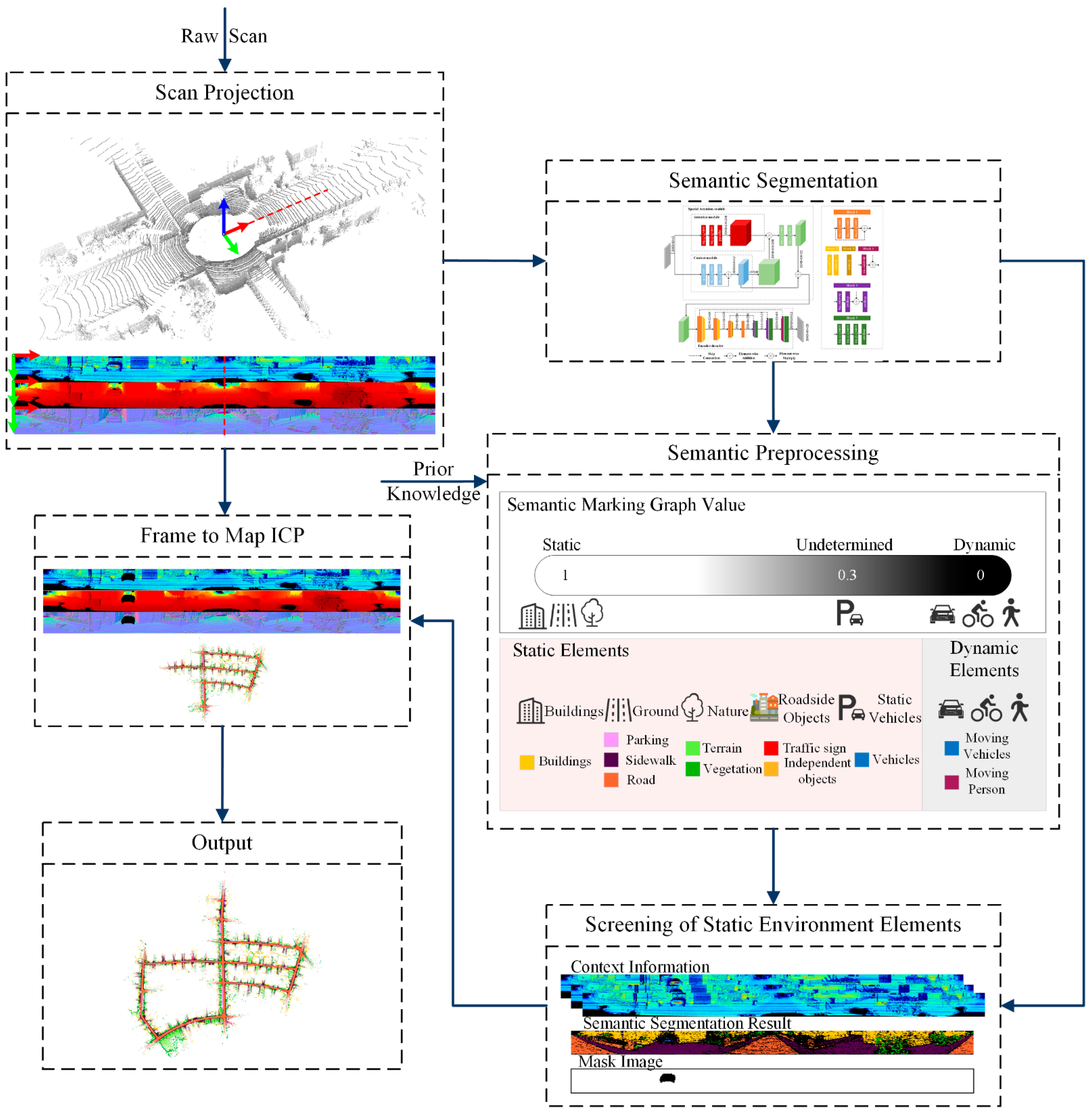
Based on SuMa++, the proposed approach applies a new dynamic object processing strategy to achieve more efficient and accurate pose estimation. The framework is shown in Figure 3. The module for the projection of point cloud data realises the projection of the point cloud data and the generation of the depth map and the normal vector map. A spherical projection [45] is used on the 3D LiDAR data to obtain the projected image (also called the range image), depth map , and normal vector map . The image-based semantic segmentation method is used in the semantic segmentation process, and is used as the input of SANet to obtain the semantic segmentation result . The dynamic element screening module realises the accurate coarse-to-fine classification of dynamic and static objects according to the context information, and obtains the semantic marking graph , which is the basis for pose estimation and semantic map construction. By adding semantic constraints to the frame-to-map ICP algorithm, the map construction module obtains accurate pose estimation results and generates a surfel map with better semantic consistency.
3.2. Semantic Segmentation
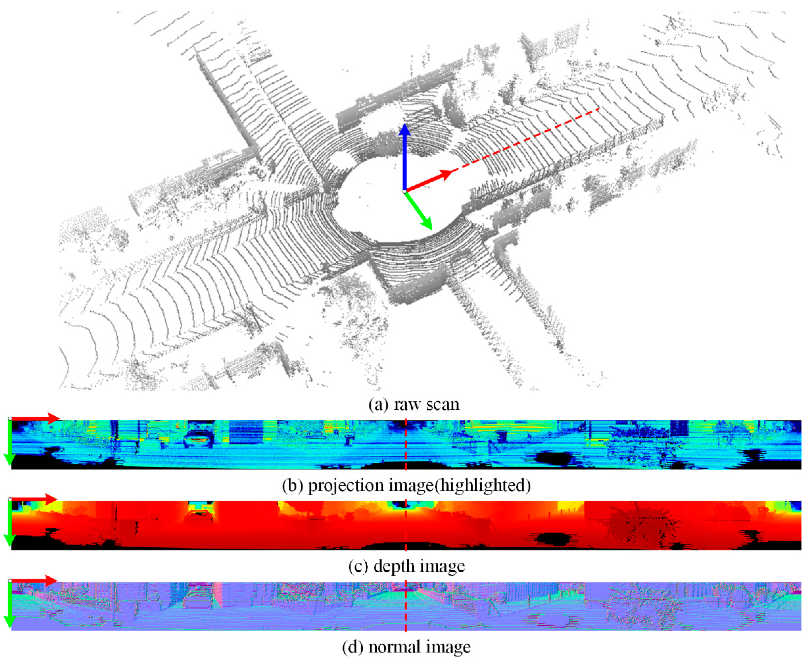
Semantic segmentation is the basic work for dynamic feature selection. Considering the current research progress on semantic segmentation of 3D point clouds and the realistic demand of LiDAR-based SLAM, image-based point cloud semantic segmentation is adopted. This method projects each 3D point in the space as one pixel on the plane for semantic segmentation. There are two reasons for choosing this method. (1) The results of image-based semantic segmentation are significantly better than those of point-based semantic segmentation in terms of performance, efficiency, and dataset training. (2) In pose estimation, due to the reduction in data dimensions, the efficiency of the traversal method based on adjacent pixels of the image is better than that of the nearest neighbour searching and matching on 3D point clouds. By performing a spherical projection on point cloud in each frame, the projected image is obtained, as shown in Figure 4. Each point on the point cloud corresponds to the pixel on the projected image I as follows:
where ; and , respectively, refer to the upper and lower limits of the vertical field of view of the LiDAR; is the width of the projected image, whose value is inversely proportional to the horizontal resolution of the LiDAR; is the height of the projected image, which is the number of LiDAR threads. This projection function guarantees that the adjacent points of any point on the 3D point cloud are still neighbouring pixels of pixel after projection, and the efficiency of the nearest neighbour searching is significantly improved.
Based on the projected image , the normal vector of each pixel is calculated by the vector cross product, and the normal vector map is obtained as follows:
It should be noted that, due to the spherical projection characteristics and the methods for acquiring the width and height of obtained projected image, the left and right boundaries of the projected image are connected in the original point cloud data, i.e., the object may be divided into two parts and appears on the left and right sides of the projected image at the same time, while the upper and lower boundaries of the projected image are determined by the vertical field of view of the LiDAR such that there is no connection between the upper and lower boundaries. Considering the above characteristics, the following processing scheme is adopted when calculating the normal vector in the boundary area of the projected image:
For each point on the 3D point cloud, we store its coordinates, its range , its remission (so-called intensity value) in the corresponding to create a [] tensor as input. We design a semantic segmentation network SANet for a LiDAR point cloud based on a spatial attention mechanism. To improve the semantic segmentation of the projected image, the feature distribution of the projected image is analysed using SqueezeSegv3 [9]. The projected image is sampled at equal intervals, and nine points are selected to analyse the coordinate distribution of the image. Comparison with the colour distribution of natural images in the COCO2017 and CIFAR10 datasets shows that the feature distribution of natural images is independent of the spatial position, whereas that of the projected image has strong spatial priori information. SqueezeSegv3 designs a spatial adaptive convolution module based on the spatial prior characteristics of the projected image to improve the adaptive performance of the convolution filter for local feature extraction.
Based on the spatial priori result of SqueezeSegv3, the projected image and its semantic segmentation method are further analysed, considering the characteristics of context relevance and spatial distribution regularity of the projected image. Context relevance is mainly reflected in the relationship between vehicles and roads (or parking areas). Vehicles are associated with roads (parking areas) in images; that is, the maximum probability for pixels around vehicles belongs to the semantic category of roads or parking areas. The spatial distribution regularity show that the environmental elements have specific spatial distribution characteristics. When the vehicle-borne LiDAR collects data, the pixel probability is centred around the vehicle’s position. The projected image based on the point cloud data obtained by this collection method directly shows that the probability of road pixels is distributed along the central axis and bottom line of the projected image, corresponding to an inverted T-shaped distribution. In addition, the characteristics of the urban environment determine the distribution of vegetation and buildings on both sides of the road, which are likely to be located on the left and right sides of the upper part of the projected image.
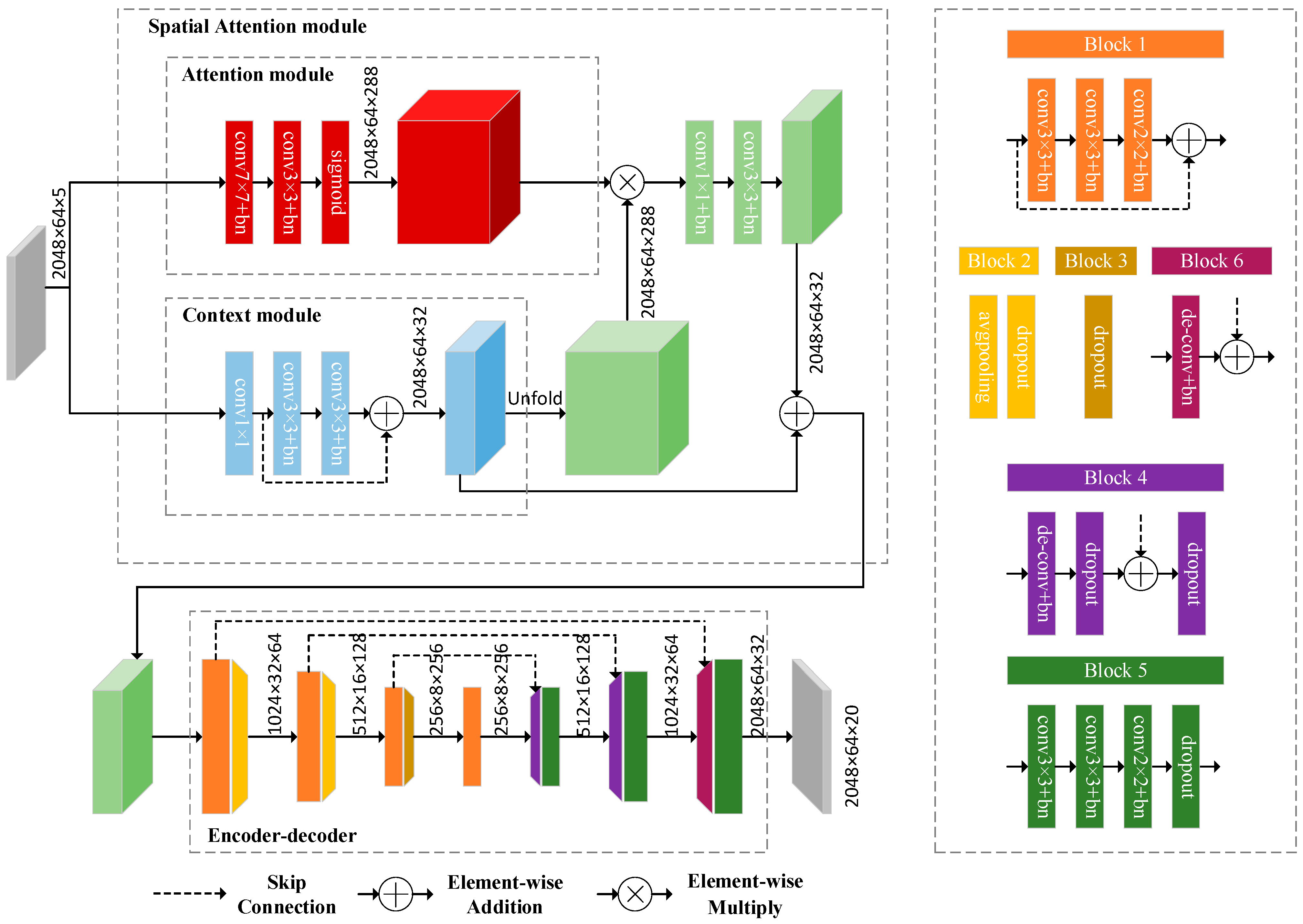
The spatial priori, context relevance, and spatial distribution regularity of a projected image are referred to as “strong spatial correlation” in this paper. We use this “strong spatial correlation” to propose a “spatial attention” module, which is used to design and implement the semantic segmentation network SANet of the LiDAR point cloud. The network structure is shown in Figure 5.
SANet is composed of a spatial attention module and a codec module. The spatial attention module is composed of an attention module and a context module. The features extracted by the spatial attention module are used as the input of codec to realise semantic segmentation of the point cloud. The attention module is designed to use a larger receptive field to obtain spatial distribution information and learns important features while excluding irrelevant features. The context module uses different receptive fields to aggregate context information and fuse different receptive fields, which enables more detailed context information to be captured. The spatial attention module aggregates spatial distribution information and context information to obtain better spatial features. The codec is based on ResNet [46] and consists of four encoders and three decoders. Each block employs a leaky-ReLU activation function, which is followed by batch normalization to make internal covariate shift reduction. The average pooling method is used to create a lighter model that meets the real-time requirements. The final feature map is finally passed to a soft-max classifier to compute pixelwise classification scores.
We use semantic segmentation in SANet to comparatively analyse the predefined environmental element classification methods on the SemanticKITTI and SemanticPOSS datasets based on a guiding ideology of map element classification and grading. The environmental elements are classified into six categories in this study (“buildings”, “ground”, “nature”, “vehicles”, “roadside objects”, and “human and animal”) and 14 subcategories (“buildings”, “parking”, “road”, “sidewalk”, “other-ground”, “vegetation”, “terrain”, “car”, “other-vehicle”, “independent objects”, “traffic-sign”, “pedestrian”, “rider”, and “animal”). Based on this classification method, the weight of each category is established as a priori knowledge for the screening of environmental elements. Although reducing the number of categories does not improve the speed and accuracy of semantic segmentation, fewer semantic annotation colours can effectively improve the calculation of average displacement in the dynamic element screening, which is discussed in Section 3.3.
3.3. Dealing with Potential Dynamics
Currently, the semantic segmentation result, where the object category is used as the output, is important information that helps the robot understand the environment at the semantic level. Hence, in this study, it is used as an important basis for the robot to determine the dynamic and static elements in the environment. From the perspective of human spatial cognition, when people come to an unfamiliar area, they pay attention to the environmental characteristics that do not change much over time, such as representative buildings and road signs, which are generally called the static information, and ignore the dynamic information, such as pedestrians and vehicles. This selective attention helps people quickly become familiar with unfamiliar areas and achieve positioning and navigation planning in those environments. Based on the current technological development, we hope to give a robot the ability to identify stable static elements in a complex and dynamic environment under the constraint of semantic information and accordingly, to build a reliable environment map. According to the characteristics of human spatial cognition in the real environment, the dynamic quantitative indexes for the environmental elements of 6 major categories and 14 subcategories are established, with corresponding values ranging from 0 to 1, from dynamic to static elements, shown in Figure 6. To distinguish the dynamic and static elements more accurately in the environment and to provide features with better robustness for the SLAM pose estimation, the environmental elements are determined based on the upper and lower thresholds. Obviously, the elements below the static threshold and above the dynamic threshold can be easily determined, and the environmental elements between the static threshold and the dynamic threshold are called semi-dynamic elements, which must be addressed.
Semi-dynamic environmental elements usually have the following characteristics: They have dynamic properties but are static in the environment for a certain period. In an urban environment, for example, a vehicle parked on the roadside for a short time or a long time satisfies the above characteristics. For environmental elements with dynamic attributes in the environment, if they are roughly classified as moving objects, the accuracy and robustness of pose estimation could be affected, resulting in a large deviation in the solution due to the sharp decrease in the number of features and the weakening of the corresponding relation between adjacent frames. To determine the static elements more accurately in the environment (regardless of whether their attributes are dynamic or static), an environmental element screening algorithm is designed and applied.
The transformation relation of points with the same name between adjacent frames is expressed as , where includes the rotation matrix and the translation vector . Correspondingly, the transformation relation of projection pixels between adjacent frames can be expressed as . represents the global coordinate system, and the overall pose transformation is as follows:
To accurately use static environment elements for pose estimation, a semantic marking graph is introduced. This marking graph is a 2D matrix, with a size of , which is the same as that of the projected image , the semantic segmentation map , and the normal vector map . The initial value of the semantic marking graph is assigned based on quantitative indexes. For pixels of static elements, the value of the semantic marking graph is 1; for pixels of dynamic elements, it is 0; and for pixels of undetermined elements, it is 0.3 as follows:
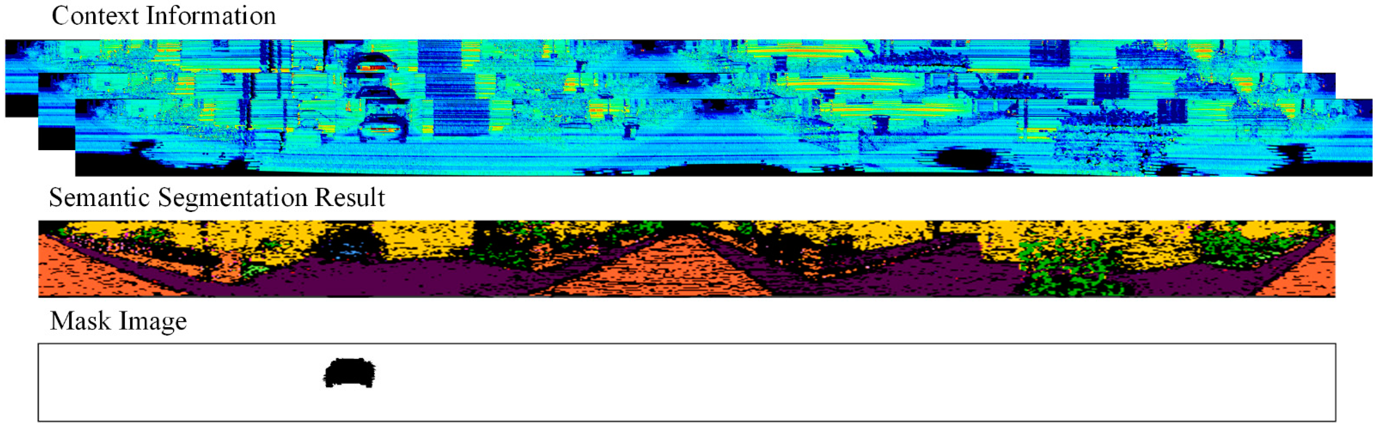
Based on the semantic marking graph, the state (dynamic or static) of each undetermined element is determined based on the contextual information of the scene. The contextual information of the scene contains the information between adjacent frames and the cross-validation information contained in the current frame. The information in the current frame reflects the process of cross-validation. For example, for a frame with the road and vehicle, the determination of the static road and the dynamic vehicle can be obtained; or for a frame with the parking area and vehicle, the determination of the static parking area and the static vehicle can be obtained. For the determination of dynamic elements in the information between adjacent frames, an algorithm for screening environmental elements is designed and applied. First, the average pixel displacement of the static elements between adjacent frames is calculated.
The symbol ⊙ is the dot product operator, i.e., the corresponding elements of two matrices are multiplied. and are the width and height of the semantic segmentation image, respectively. are the semantic segmentation images and semantic marking graphs between adjacent scans, respectively. We assume that the pose is not significantly changed between adjacent frames, and under the condition that no accurate pose estimation is obtained, the pose transformation parameter of the previous frame is used as the initial value to calculate the pixel average displacement. Then, a threshold according to the average displacement is set to determine the state of each undetermined element and update the semantic marking graph as follows:
where is the threshold weight and classifies pixels meeting this constraint as static elements, and the corresponding semantic marking graph is updated () to obtain the semantic marking graph at time . The screening of environmental elements based on context information is shown in Figure 7. Algorithm 1 shows the environmental element screening algorithm.
| Algorithm 1. Screening of static environment elements |
| Input: pose transformation matrix , semantic segmentation result |
| and semantic marking graph |
| Output: updated semantic marking Graph |
| Intermediate variable: average displacement and decision weight |
| Begins |
| for i in w, do |
| for j in h, do |
| calculate ; |
| end |
| end |
| for u in w, do |
| for v in h, do |
| if then |
| else |
| end |
| end |
3.4. Pose Estimation
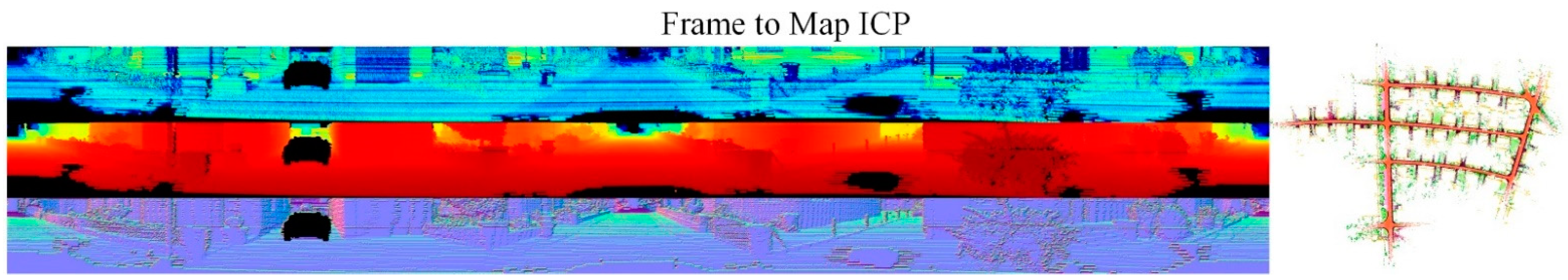
Pose estimation is usually described as a nonlinear optimisation problem. Considering the characteristics of the surfel map, the frame-to-map ICP under semantic constraints is adopted. With the help of the semantic marking graph , the static elements in the environment can be accurately used for pose estimation. Figure 8 shows an example of the frame-to-map ICP based on semantic constraints.
The function for error minimisation is defined as follows:
where are the projection images and semantic marking graphs between adjacent scans, respectively. is the normal map at time . For every iteration of the frame-to-map ICP, the 6-DoF relative pose is incrementally updated using Levenberg–Marquardt as follows [47]:
where Jacobian and residual are functions of the normal map . The diagonal matrix is used for regularisation of the Hessian matrix with . The weight matrix is a diagonal matrix containing weights for each residual . Once the frame-to-map ICP reaches a stopping criterion (e.g., max. number of iterations), the relative transformation matrix is computed from and used to output the desired map-aligned pose as Equation (5).
Within frame-to-map ICP, we set up the weight for the considering the direction of the advance of the LiDAR based on the semantic marking graph. The semantic marking graph filters out dynamic elements in the environment during registration and pose estimation without using all pixel information, and there is no need to set weights for the iteration of dynamic and static elements. Therefore, with the help of a semantic marking graph, the weight setting principle is correlated with the forward direction of the LiDAR sensors, i.e., the weights of the pixels facing the forward direction are higher than those of the pixels facing the lateral and backward directions. For the map construction and determination of position and pose, the scanning data in the forward direction can provide significantly higher gain than those in the lateral and backward directions. In other words, the data in the forward direction are the newly acquired real data, while the data in the lateral and backward directions are similar to the scanning data of the previous frame. Therefore, the LiDAR point cloud data are divided into three equal parts according to the angle. For convenience of calculations, the imaging interval of the projected image in the forward direction is set at . As shown in Figure 9, the weight matrix for pose estimation is obtained.
4. Experiments
In this section, we evaluate our approach on the public datasets SemanticKITTI [48], KITTI [49], and SemanticPOSS [50]. First, the SemanticKITTI dataset is used to verify the performance of SANet. SANet is trained using a hardware platform with an 8 GeForce RTX™ 2080 Ti GPU for 150 epochs. Then, experiments are performed to verify the proposed SLAM method for dynamic environments. The dynamic environment places high requirements on the stability and accuracy of the SLAM algorithms. To verify the effectiveness of the proposed approach, two different outdoor environment LiDAR datasets are selected. The KITTI dataset is the evaluation benchmark for many SLAM algorithms. Experiments on this dataset can test the performance of the proposed approach and facilitate a horizontal comparison with other algorithms. The SemanticPOSS and KITTI datasets are quite different in terms of the collection equipment, collection locations, and data content. The experiments based on the SemanticPOSS dataset confirm the robustness and stability of the proposed approach in the longitudinal direction. To demonstrate the results of our approach in dynamic environments, we compare it with other state-of-the-art LiDAR SLAM systems or with visual SLAM systems. Our experiments are developed on a PC with an Intel i7-9700k CPU, 16 GB RAM, and a single GeForce RTX™ 2080 Ti GPU.
4.1. Semantic Segmentation Experiments on the SemanticKITTI Dataset
To fully evaluate the performance of SANet against other semantic segmentation algorithms using a unified benchmark, we select the SemanticKITTI dataset for training, verification, and testing. The SemanticKITTI dataset provides 43,442 frames of point cloud data (sequence 00–10 contains point cloud data annotation). The semantic segmentation challenge is launched on the official website of the dataset to evaluate the test data using unified indicators. Based on the requirements of other algorithms and datasets, 19,130 frames of point cloud data of sequences 00–07 and 09–10 are used as the training dataset, 4071 frames of sequence 08 are used as the verification dataset, and 20,351 frames of sequence 11–21 are used as the test dataset. The dataset used for the semantic segmentation of single frame data has 19 categories and is evaluated on the official platform. The evaluation index is the mIoU (mean intersection-over-union):
C denotes the number of categories, and denote the true positive, false positive, and false negative values of category , respectively. After training, semantic segmentation is performed on the test dataset, and the results are uploaded to the semantic segmentation challenge of the SemanticKITTI official website for evaluation. Table 1 presents a comparison of the quantitative evaluation results of SANet on the test dataset against those of four other algorithms (RangeNet53++ and SqueezeSegV3 are abbreviated as RangeNet and SquSegV3, respectively).
SANet improves the mIoU score by at least 3.3% on the basis of ensuring real-time performance (which is slightly lower than that of SalsaNet [51] and SalsaNext [52]). SANet achieved a 59.2% mIoU score on the SemanticKITTI test set, which fully proves the proposed feature extraction method based on the spatial attention mechanism efficiently aggregates the local features of different receptive fields and significantly improves the accuracy of semantic segmentation after encoding and decoding.
4.2. KITTI Dataset
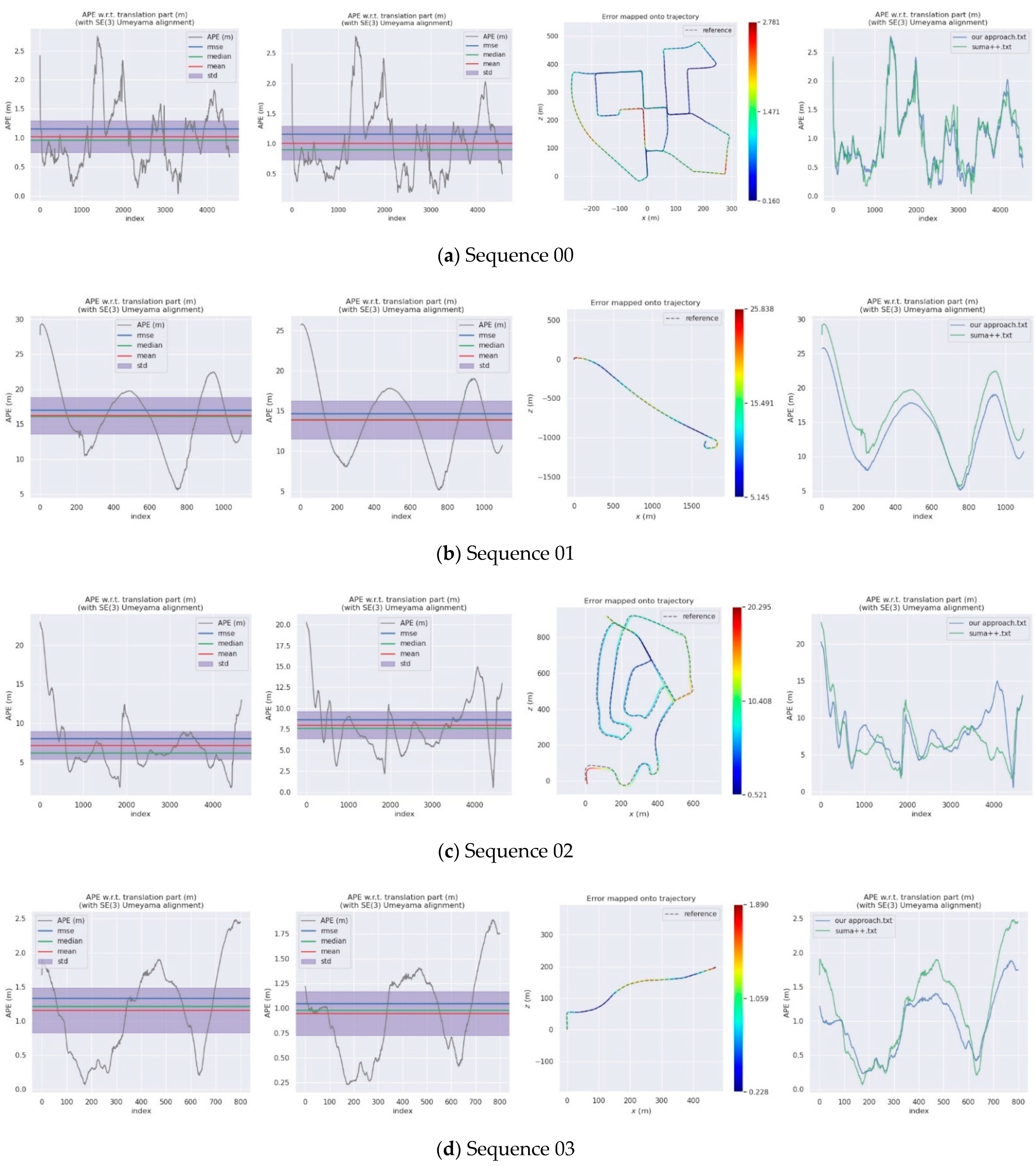
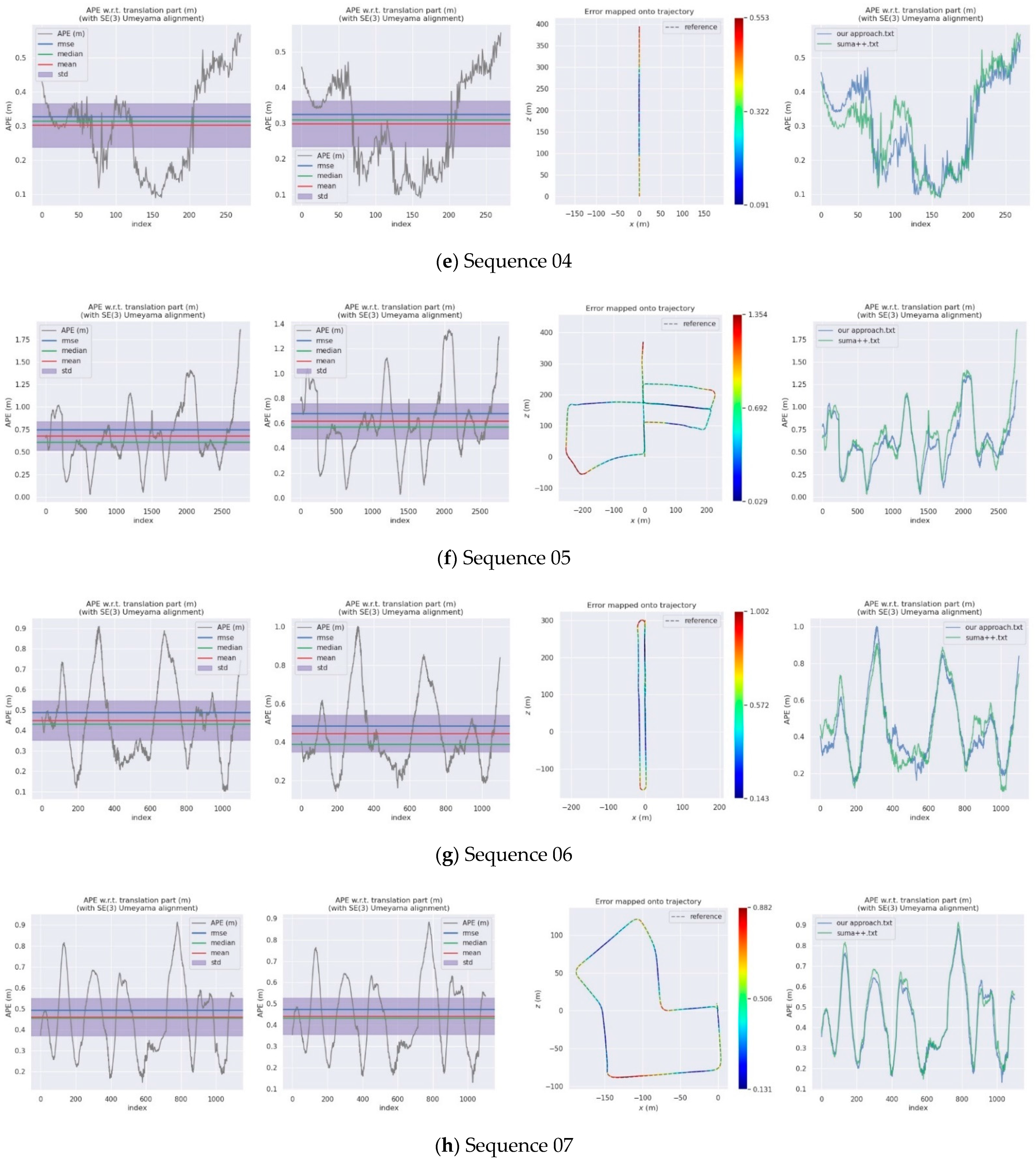
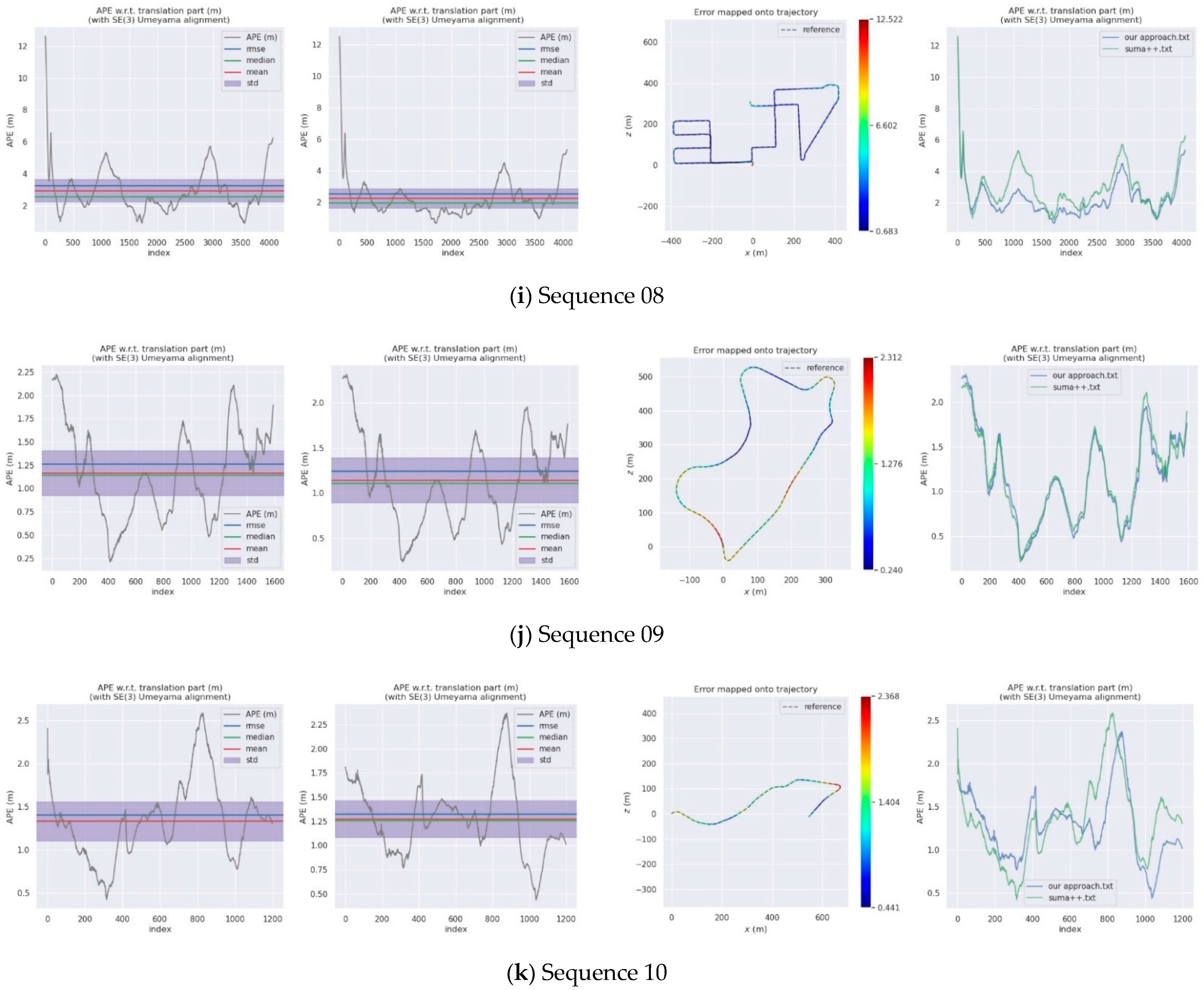
The KITTI dataset is collected by Velodyne HDL-64E and has been the mainstream dataset for SLAM algorithm evaluation since its release. It contains 11 sets of data in typical outdoor environments, e.g., urban, highway and rural environments, which can reflect the characteristics of dynamic environments. In addition, most of the dynamic objects in outdoor environments covered by the KITTI dataset are static, which can better test the performance of the proposed algorithm for screening environmental elements.
For the evaluation of the SLAM algorithm, the quantitative evaluation index of absolute pose error (APE) is applied, using Sim (3) Umeyama alignment in the calculation. We then use the evo tool [53] to evaluate the estimated pose results, including the root mean square error (RMSE), the mean error, the median error, and the standard deviation (Std.). The SuMa++ algorithm based on LiDAR data and the DynaSLAM and DM-SLAM [54], two visual SLAM algorithms with excellent performance in dynamic environments, are selected for comparisons, since the proposed approach draws on the idea of image masking from DynaSLAM. Table 2 is a comparison of the APE used for the translation component of different algorithms and provides details of our approach. Figure 10 shows the results of the error mapped onto the trajectory by our approach and the APE visualisation results between SuMa++ and our approach. Figure 11 shows the semantic map of the sequence 00, 05, 08. In the comparison with the visual SLAM methods, the proposed approach made significant progress on the six sequence data and is inferior to the visual SLAM methods for the other five sequence data. In the comparison with SuMa++, the proposed approach made significant progress in the six sequence data and little improvement in the four sequence data; however, the performance decreases on the Sequence 02 data. Considering that most of the dynamic objects in the KITTI data set are static in the environment, the experimental results strongly demonstrate the effectiveness of the environmental element selection algorithm, which improves the accuracy of pose estimation and enhances the robustness of the SLAM system.
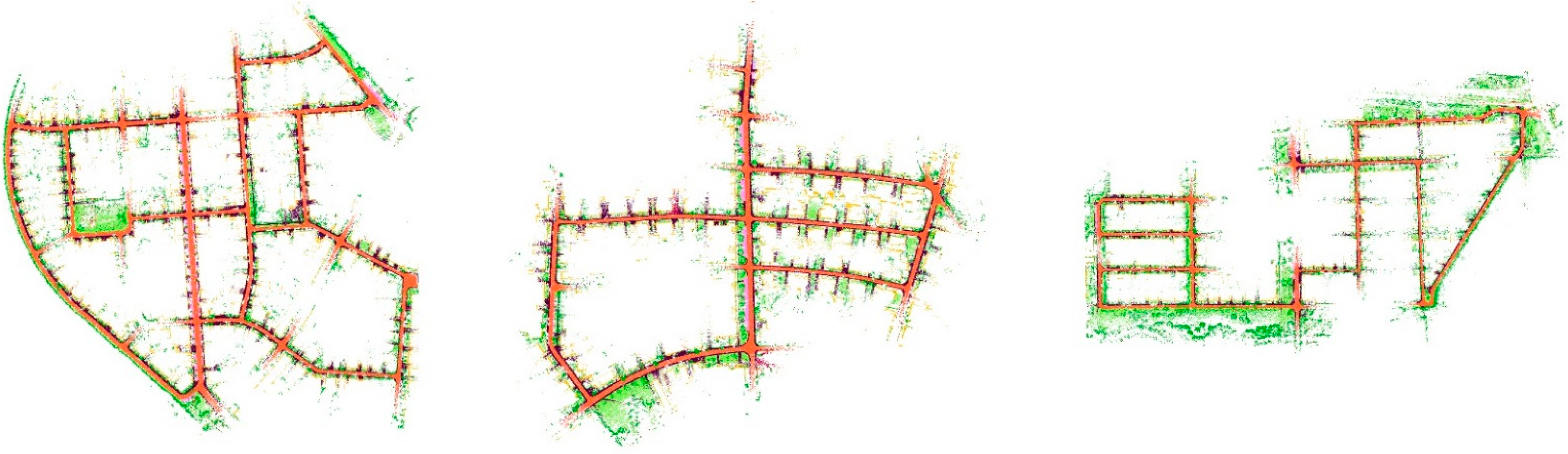
4.3. SemanticPOSS Dataset
The SemanticPOSS dataset is composed of six groups of campus environmental data collected by Hesai Pandora LiDAR. Table 3 shows the comparison results of the dynamic elements between SemanticPOSS and other mainstream outdoor datasets [49]. Compared with the KITTI dataset in which most dynamic objects are static in the environment, the SemanticPOSS dataset, which is small in size, covers more dynamic elements and is more in line with the characteristics of dynamic environments. In addition, the truth trajectory of six groups of data in the SemanticPOSS dataset is relatively stable without a closed loop; thus, the SemanticPOSS dataset can be used for testing the accuracy and robustness of the SLAM algorithm in a highly dynamic environment.
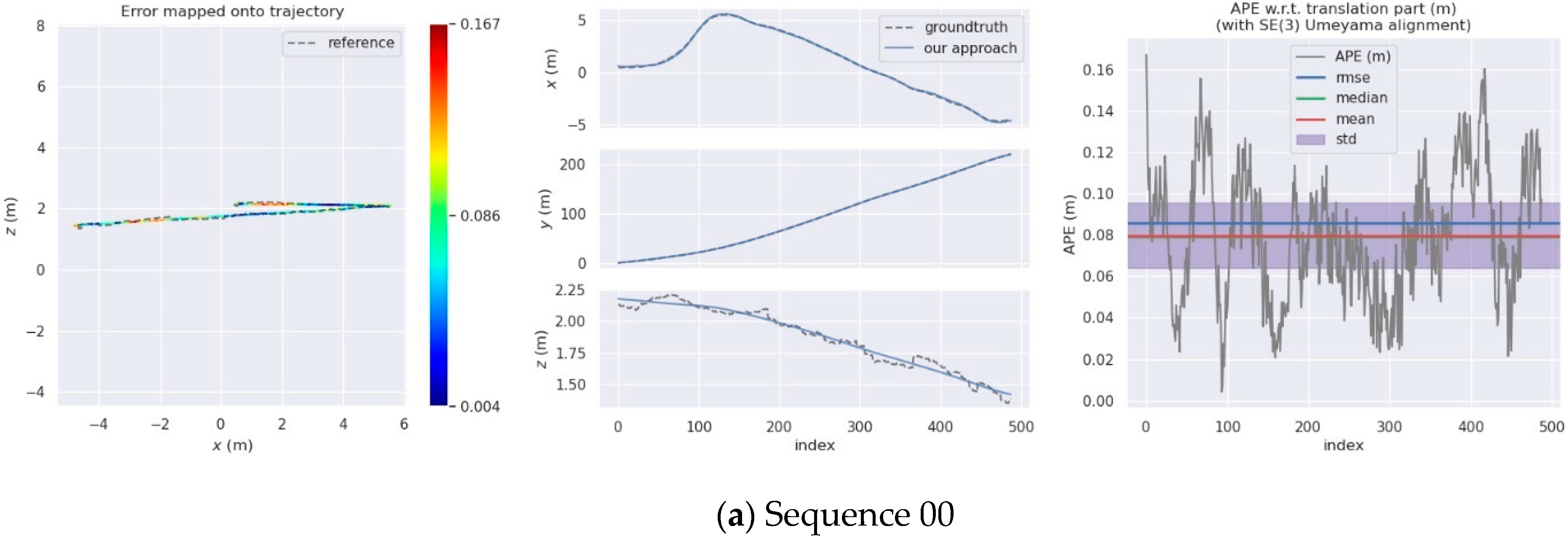
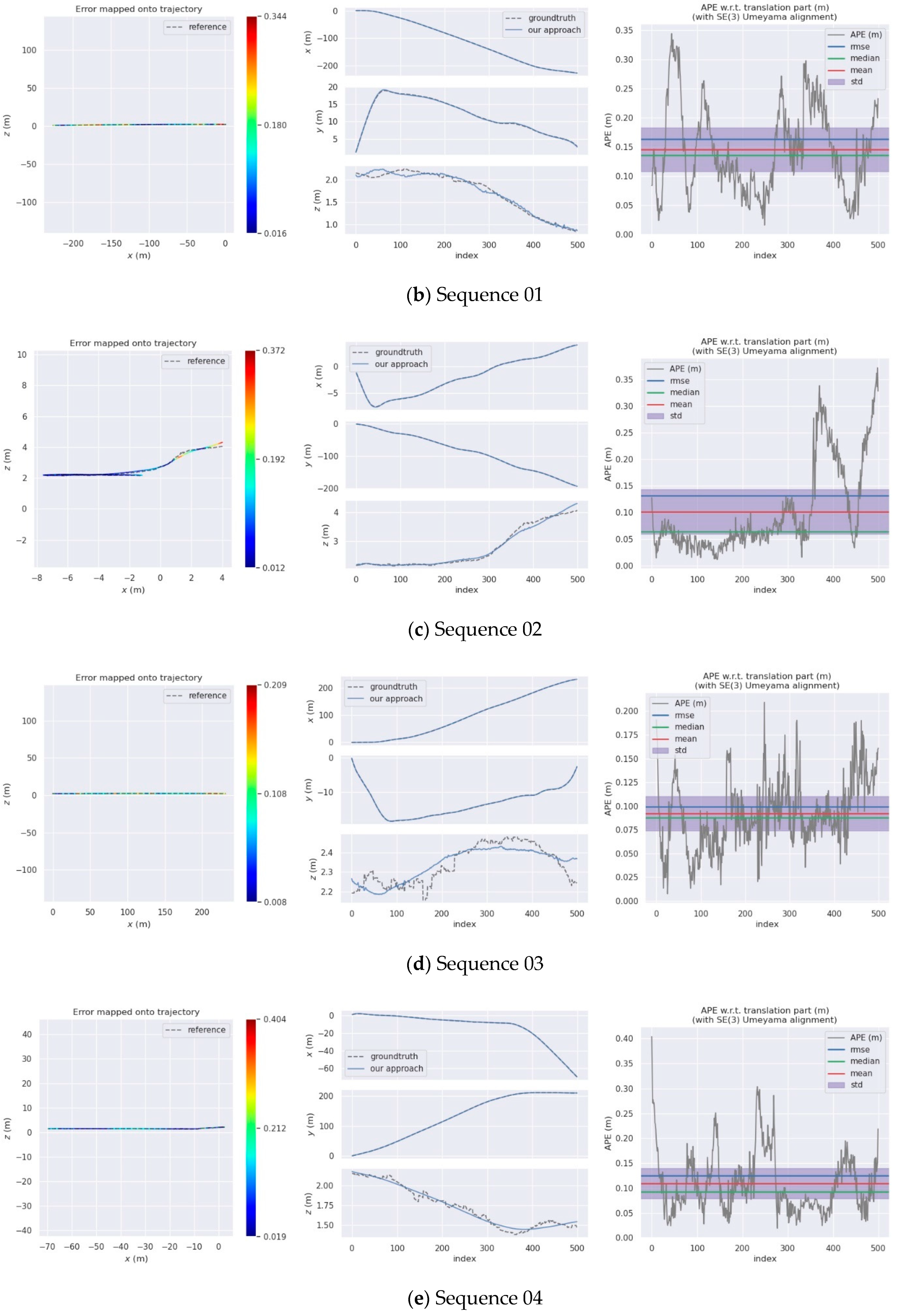
Because SuMa++ can only be implemented in the KITTI dataset and cannot be implemented in the SemanticPOSS dataset, only the proposed approach is quantitatively evaluated. Experiments are conducted on the six groups of data in the SemanticPOSS dataset. Table 4 shows that the proposed approach achieves relatively excellent results. Figure 12 shows the visualisation results. Good pose estimation results are obtained in the x and y directions, but there is deviation in the z direction, which is the main cause of inaccurate pose estimation. The deviation in the z direction is caused by the dimensionality reduction during the projection of the acquired point cloud data into the projected image. The dimensionality reduction of 3D data into a 2D image inevitably leads to loss of information. Although the depth map and normal vector map are improved, there are still errors.
Overall, experiments on the KITTI and the SemanticPOSS datasets demonstrate that the proposed approach effectively eliminates the interference of dynamic elements in the environment, improves the accuracy of pose estimation, enhances the performance of SLAM, and obtains excellent results.
5. Conclusions
In this paper, a LiDAR-based SLAM framework is constructed under the constraint of semantic information. The performance of the LiDAR-based SLAM is improved by using the environmental element screening algorithm in dynamic environments. This framework is divided into four modules, i.e., projection of point cloud data, semantic segmentation, dynamic element screening, and semantic map construction. The proposed approach is inspired by SuMa++ and DynaSLAM. There are three main contributions of this approach. First, a semantic segmentation method SANet for LiDAR point clouds based on spatial attention mechanism is proposed that effectively improves the real-time performance and accuracy of semantic segmentation. Second, a dynamic element selection algorithm that considers context information is proposed that simply and effectively improves the robustness and accuracy of dynamic element determination. Third, a LiDAR-based SLAM framework in a dynamic environment is constructed and used with semantic segmentation and prior knowledge to realise real-time localisation and semantic map construction in dynamic environments.
This framework is evaluated on three datasets, namely, SemanticKITTI, KITTI, and SemanticPOSS. An experiment is performed on the SemanticKITTI dataset, and better semantic segmentation results are achieved than by using other excellent semantic segmentation networks. The experiment on the KITTI dataset achieves a horizontal comparison with other excellent SLAM algorithms. The performance of the proposed framework is better than that of SuMa++, a LiDAR-based SLAM, and is partially better than that of visual SLAM methods, such as DM-SLAM and DynaSLAM. The experiment in highly dynamic environments is conducted on the SemanticPOSS dataset, and accurate pose estimation results are obtained. The experimental results show that the proposed approach has reliable performance, accuracy, and robustness in dynamic environments.
In summary, we explored LiDAR-based SLAM in dynamic environments in this study, and we will investigate point cloud semantic segmentation and LiDAR-based SLAM in more complex dynamic environments in the future.
Author Contributions
Conceptualization, W.W. and X.Y.; formal analysis, W.W. and X.Y.; methodology, W.W., X.Y., X.Z. and L.C.; software, W.W., X.Z., L.Z. and X.L.; supervision, L.C.; validation, L.Z. and X.L.; writing—original draft, W.W., X.Z., and L.C.; writing—review and editing, X.Y., L.Z. and X.L. All authors have read and agreed to the published version of the manuscript.
Funding
This research was funded by the National Natural Science Foundation of China (Project No.42130112 and No.42171456), the Youth Program of the National Natural Science Foundation of China (Project No.41801317), the Central Plains Scholar Scientist Studio Project of Henan Province, the National Key Research and Development Program of China (Project No.2017YFB0503500).
Institutional Review Board Statement
Not applicable.
Informed Consent Statement
Not applicable.
Data Availability Statement
Our experimental data are all open-source data sets.
Conflicts of Interest
The authors declare no conflict of interest.
References
- The Group of Strategic Research on Artificial Intelligence 2.0 in China. In Strategic Research on Artificial Intelligence 2.0 in China; Zhejiang University press: Zhejiang, China, 2018; pp. 1–10.
- Jun, G.A.O. The 60 Anniversary and Prospect of Acta Geodaetica et Cartographica Sinica. Acta Geod. Et Cartogr. Sin. 2017, 46, 1219–1225. [Google Scholar]
- Gao, B.; Pan, Y.; Li, C.; Geng, S.; Zhao, H. Are We Hungry for 3D LiDAR Data for Semantic Segmentation? A Survey of Datasets and Methods. IEEE Trans. Intell. Transp. Syst. 2021, 1–19. [Google Scholar] [CrossRef]
- Qi, C.R.; Yi, L.; Su, H.; Guibas, L.J. PointNet++ deep hierarchical feature learning on point sets in a metric space. In Proceedings of the 31st International Conference on Neural Information Processing Systems, Long Beach, CA, USA, 3–9 December 2017; pp. 5105–5114. [Google Scholar]
- Li, Y.; Bu, R.; Sun, M.; Wu, W.; Di, X.; Chen, B. Pointcnn: Convolution on x-transformed points. Advances in neural information processing systems. Adv. Neural Inf. Process. Syst. 2018, 31, 820–830. [Google Scholar]
- Lawin, F.J.; Danelljan, M.; Tosteberg, P.; Bhat, G.; Khan, F.S.; Felsberg, M. Deep projective 3D semantic segmentation. In Proceedings of the International Conference on Computer Analysis of Images and Patterns, Ystad, Sweden, 22–24 August 2017; Springer: Cham, The Netherlands, 2017; pp. 95–107. [Google Scholar]
- Wu, B.; Wan, A.; Yue, X.; Keutzer, K. Squeezeseg: Convolutional neural nets with recurrent crf for real-time road-object segmentation from 3d lidar point cloud. In Proceedings of the 2018 IEEE International Conference on Robotics and Automation (ICRA), Brisbane, QLD, Australia, 21–25 May 2018; pp. 1887–1893. [Google Scholar]
- Wu, B.; Zhou, X.; Zhao, S.; Yue, X.; Keutzer, K. Squeezesegv2: Improved model structure and unsupervised domain adaptation for road-object segmentation from a lidar point cloud. In Proceedings of the IEEE 2019 International Conference on Robotics and Automation (ICRA), Montreal, QC, Canada, 20–24 May 2019; pp. 4376–4382. [Google Scholar]
- Xu, C.; Wu, B.; Wang, Z.; Zhan, W.; Vajda, P.; Keutzer, K.; Tomizuka, M. Squeezesegv3: Spatially-adaptive convolution for efficient point-cloud segmentation. In European Conference on Computer Vision; Springer: Cham, The Netherlands, 2020; pp. 1–19. [Google Scholar]
- Milioto, A.; Vizzo, I.; Behley, J.; Stachniss, C. Rangenet++: Fast and accurate lidar semantic segmentation. In Proceedings of the 2019 IEEE/RSJ International Conference on Intelligent Robots and Systems (IROS), Macau, China, 4–8 November 2019; pp. 4213–4220. [Google Scholar]
- Liu, F.; Li, S.; Zhang, L.; Zhou, C.; Ye, R.; Wang, Y.; Lu, J. 3DCNN-DQN-RNN: A deep reinforcement learning framework for semantic parsing of large-scale 3D point clouds. In Proceedings of the IEEE International Conference on Computer Vision, Venice, Italy, 22–29 October 2017; pp. 5678–5687. [Google Scholar]
- Radi, H.; Ali, W. VolMap: A Real-time Model for Semantic Segmentation of a LiDAR surrounding view. arXiv 2019, arXiv:1906.11873. [Google Scholar]
- Cadena, C.; Carlone, L.; Carrillo, H.; Latif, Y.; Scaramuzza, D.; Neira, J.; Reid, I.; Leonard, J.J. Past, Present, and Future of Simultaneous Localization and Mapping: Toward the Robust-Perception Age. IEEE Trans. Robot. 2016, 32, 1309–1332. [Google Scholar] [CrossRef] [Green Version]
- Yu, C.; Liu, Z.; Liu, X.-J.; Xie, F.; Yang, Y.; Wei, Q.; Fei, Q. DS-SLAM: A Semantic Visual SLAM towards Dynamic Environments. In Proceedings of the 2018 IEEE/RSJ International Conference on Intelligent Robots and Systems (IROS), Madrid, Spain, 1–5 October 2018; pp. 1168–1174. [Google Scholar]
- Zeng, Z.; Zhou, Y.; Jenkins, O.C.; Desingh, K. Semantic mapping with simultaneous object detection and localization. In Proceedings of the 2018 IEEE/RSJ International Conference on Intelligent Robots and Systems (IROS), Madrid, Spain, 1–5 October 2018; pp. 911–918. [Google Scholar]
- Sünderhauf, N.; Dayoub, F.; McMahon, S.; Talbot, B.; Schulz, R.; Corke, P.; Wyeth, G.; Upcroft, B.; Milford, M. Place categorization and semantic mapping on a mobile robot. In Proceedings of the 2016 IEEE International Conference on Robotics and Automation (ICRA), Stockholm, Sweden, 16–21 May 2016; pp. 5729–5736. [Google Scholar]
- Mousavian, A.; Toshev, A.; Fišer, M.; Košecká, J.; Wahid, A. Visual representations for semantic target driven navigation. In Proceedings of the 2019 International Conference on Robotics and Automation (ICRA), Montreal, QC, Canada, 20–24 May 2019; pp. 8846–8852. [Google Scholar]
- Ma, W.C.; Tartavull, I.; Bârsan, I.A.; Wang, S.; Bai, M.; Mattyus, G.; Homayounfar, N.; Lakshmikanth, S.K.; Pokrovsky, A.; Urtasun, R. Exploiting Sparse Semantic HD Maps for Self-Driving Vehicle Localization. In Proceedings of the 2019 IEEE/RSJ International Conference on Intelligent Robots and Systems (IROS), Macau, China, 4–8 November 2019; pp. 5304–5311. [Google Scholar]
- Limketkai, B.; Liao, L.; Fox, D. Relational object maps for mobile robots. In Proceedings of the Nineteenth International Joint Conference on Artificial Intelligence (IJCAI), Edinburgh, Scotland, UK, 30 July–5 August 2005; pp. 1471–1476. [Google Scholar]
- Nüchter, A.; Hertzberg, J. Towards semantic maps for mobile robots. Robot. Auton. Syst. 2008, 56, 915–926. [Google Scholar] [CrossRef] [Green Version]
- Sengupta, S.; Sturgess, P.; Torr, P.H.S. Automatic dense visual semantic mapping from street-level imagery. In Proceedings of the 2012 IEEE/RSJ International Conference Intelligent Robots and Systems (IROS), Vilamoura-Algarve, Portugal, 7–12 October 2012; pp. 857–862. [Google Scholar]
- Valentin, J.P.; Sengupta, S.; Warrell, J.; Shahrokni, A.; Torr, P.H. Mesh based semantic modelling for indoor and outdoor scenes. In Proceedings of the IEEE Conference on Computer Vision and Pattern Recognition, Portland, OR, USA, 23–28 June 2013; pp. 2067–2074. [Google Scholar]
- Sengupta, S.; Sturgess, P. Semantic octree: Unifying recognition, reconstruction and representation via an octree constrained higher order MRF. In Proceedings of the 2015 IEEE International Conference, Robotics and Automation (ICRA), Seattle, WA, USA, 25–30 May 2015; pp. 1874–1879. [Google Scholar]
- Long, J.; Shelhamer, E.; Darrell, T. Fully convolutional networks for semantic segmentation. In Proceedings of the IEEE Conference on Computer Vision and Pattern Recognition, Boston, MA, USA, 7–12 June 2015; pp. 3431–3440. [Google Scholar]
- Chen, L.C.; Papandreou, G.; Kokkinos, I.; Murphy, K.; Yuille, A.L. Deeplab: Semantic image segmentation with deep convolutional nets, atrous convolution, and fully connected crfs. IEEE Trans. Pattern Anal. Mach. Intell. 2018, 40, 834–848. [Google Scholar] [CrossRef] [PubMed]
- Zhao, H.; Qi, X.; Shen, X.; Shi, J.; Jia, J. Icnet for real-time semantic segmentation on high-resolution images. In Proceedings of the European Conference on Computer Vision (ECCV), Munich, Germany, 8–14 September 2018; pp. 405–420. [Google Scholar]
- Badrinarayanan, V.; Kendall, A.; Cipolla, R. SegNet: A Deep Convolutional Encoder-Decoder Architecture for Image Segmentation. IEEE Trans. Pattern Anal. Mach. Intell. 2017, 39, 2481–2495. [Google Scholar] [CrossRef] [PubMed]
- Vasudevan, S.; Gächter, S.; Nguyen, V.; Siegwart, R. Cognitive maps for mobile robots—An object based approach. Robot. Auton. Syst. 2007, 55, 359–371. [Google Scholar] [CrossRef] [Green Version]
- Vasudevan, S.; Siegwart, R. Bayesian space conceptualization and place classification for semantic maps in mobile robotics. Robot. Auton. Syst. 2008, 56, 522–537. [Google Scholar] [CrossRef]
- Rituerto, A.; Murillo, A.C.; Guerrero, J.J. Semantic labeling for indoor topological mapping using a wearable catadioptric system. Robot. Auton. Syst. 2014, 62, 685–695. [Google Scholar] [CrossRef]
- Liu, M.; Colas, F.; Pomerleau, F.; Siegwart, R. A Markov semi-supervised clustering approach and its application in topological map extraction. In Proceedings of the 2012 IEEE/RSJ International Conference on Intelligent Robots and Systems, Vilamoura-Algarve, Portugal, 7–12 October 2012; pp. 4743–4748. [Google Scholar]
- Brunskill, E.; Kollar, T.; Roy, N. Topological mapping using spectral clustering and classification. In Proceedings of the 2007 IEEE/RSJ International Conference on Intelligent Robots and Systems, San Diego, CA, USA, 29 October–2 November 2007; pp. 3491–3496. [Google Scholar]
- Liu, M.; Colas, F.; Siegwart, R. Regional topological segmentation based on mutual information graphs. In Proceedings of the 2011 IEEE International Conference on Robotics and Automation. IEEE, Shanghai, China, 9–13 May 2011; pp. 3269–3274. [Google Scholar]
- Liu, Z.; Chen, D.; von Wichert, G. Online semantic exploration of indoor maps. In Proceedings of the 2012 IEEE International Conference on Robotics and Automation, Saint Paul, MN, USA, 14–18 May 2012; pp. 4361–4366. [Google Scholar]
- Pronobis, A.; Mozos, O.; Caputo, B.; Jensfelt, P. Multi-modal Semantic Place Classification. Int. J. Robot. Res. 2009, 29, 298–320. [Google Scholar] [CrossRef]
- Pronobis, A.; Jensfelt, P. Large-scale semantic mapping and reasoning with heterogeneous modalities. In Proceedings of the 2012 IEEE International Conference on Robotics and Automation, Saint Paul, MN, USA, 14–18 May 2012; pp. 3515–3522. [Google Scholar]
- Goeddel, R.; Olson, E. Learning semantic place labels from occupancy grids using CNNs. In Proceedings of the 2016 IEEE/RSJ international conference on intelligent robots and systems (IROS), Daejeon, Korea, 9–14 October 2016; pp. 3999–4004. [Google Scholar]
- Hiller, M.; Qiu, C.; Particke, F.; Hofmann, C.; Thielecke, J. Learning Topometric Semantic Maps from Occupancy Grids. In Proceedings of the 2019 IEEE/RSJ International Conference on Intelligent Robots and Systems (IROS), Macau, China, 4–8 November 2019. [Google Scholar]
- Saputra, M.R.U.; Markham, A.; Trigoni, N. Visual SLAM and structure from motion in dynamic environments: A survey. ACM Comput. Surv. (CSUR) 2018, 51, 1–36. [Google Scholar] [CrossRef]
- Bescos, B.; Facil, J.M.; Civera, J.; Neira, J. DynaSLAM: Tracking, Mapping, and Inpainting in Dynamic Scenes. IEEE Robot. Autom. Lett. 2018, 3, 4076–4083. [Google Scholar] [CrossRef] [Green Version]
- Xiao, L.; Wang, J.; Qiu, X.; Rong, Z.; Zou, X. Dynamic-SLAM: Semantic monocular visual localization and mapping based on deep learning in dynamic environment. Robot. Auton. Syst. 2019, 117, 1–16. [Google Scholar] [CrossRef]
- Chen, X.; Milioto, A.; Palazzolo, E.; Giguere, P.; Behley, J.; Stachniss, C. Suma++: Efficient lidar-based semantic slam. In Proceedings of the 2019 IEEE/RSJ International Conference on Intelligent Robots and Systems (IROS), Macau, China, 4–8 November 2019; pp. 4530–4537. [Google Scholar]
- Zaganidis, A.; Sun, L.; Duckett, T.; Cielniak, G. Integrating Deep Semantic Segmentation Into 3-D Point Cloud Registration. IEEE Robot. Autom. Lett. 2018, 3, 2942–2949. [Google Scholar] [CrossRef] [Green Version]
- Dubé, R.; Cramariuc, A.; Dugas, D.; Nieto, J.; Siegwart, R.; Cadena, C. SegMap: 3D Segment Mapping using Data-Driven Descriptors. In Robotics: Science and Systems XIV; MIT Press: Cambridge, MA, USA, 2018. [Google Scholar]
- Li, B.; Zhang, T.; Xia, T. Vehicle Detection from 3D Lidar Using Fully Convolutional Network. arXiv arXiv:1608.07916, 2016.
- He, K.; Zhang, X.; Ren, S.; Sun, J. Deep residual learning for image recognition. In Proceedings of the IEEE Conference on Computer Vision and Pattern Recognition, Las Vegas, NV, USA, 27–30 June 2016; pp. 770–778. [Google Scholar]
- Hinzmann, T. Perception and Learning for Autonomous UAV Missions. Ph.D. Thesis, ETH Zurich, Zürich, Switzerland, 2020. [Google Scholar]
- Behley, J.; Garbade, M.; Milioto, A.; Quenzel, J.; Behnke, S.; Stachniss, C.; Gall, J. SemanticKITTI: A Dataset for Semantic Scene Understanding of LiDAR Sequences. In Proceedings of the 2019 IEEE/CVF International Conference on Computer Vision (ICCV); Institute of Electrical and Electronics Engineers (IEEE), Seoul, Korea, 27 October–3 October 2019; pp. 9296–9306. [Google Scholar]
- Geiger, A.; Lenz, P.; Urtasun, R. Are we ready for autonomous driving? The KITTI vision benchmark suite. In Proceedings of the 2012 IEEE Conference on Computer Vision and Pattern Recognition, Providence, RI, USA, 16–21 June 2012; pp. 3354–3361. [Google Scholar] [CrossRef]
- Pan, Y.; Gao, B.; Mei, J.; Geng, S.; Li, C.; Zhao, H. SemanticPOSS: A Point Cloud Dataset with Large Quantity of Dynamic Instances. In Proceedings of the 2020 IEEE Intelligent Vehicles Symposium (IV), Las Vegas, NV, USA, 19 October–13 November 2020; pp. 687–693. [Google Scholar]
- Aksoy, E.E.; Baci, S.; Cavdar, S. Salsanet: Fast road and vehicle segmentation in lidar point clouds for autonomous driving. In Proceedings of the 2020 IEEE Intelligent Vehicles Symposium (IV), Las Vegas, NV, USA, 19 October–13 November 2020; pp. 926–932. [Google Scholar]
- Cortinhal, T.; Tzelepis, G.; Aksoy, E.E. SalsaNext: Fast, uncertainty-aware semantic segmentation of LiDAR point clouds. In International Symposium on Visual Computing; Springer: Cham, The Netherlands, 2020; pp. 207–222. [Google Scholar]
- Grupp, M. Evo: Python PackAge for the Evaluation of Odometry and Slam. Available online: https://github.com/MichaelGrupp/evo (accessed on 5 May 2021).
- Lu, X.; Wang, H.; Tang, S.; Huang, H.; Li, C. DM-SLAM: Monocular SLAM in dynamic environments. Appl. Sci. 2020, 10, 4252. [Google Scholar] [CrossRef]
Figure 1.
Object-based semantic map.

Figure 2.
Region-based semantic map.

Figure 3.
Overview of our proposed method. Input scans are projected through spherical projection and segmented by proposed SANet, then elements that fall in the assumed dynamic content by semantic pre-processing and screening algorithms are discarded for pose estimation. The static environment elements are fed into the SLAM algorithm for tracking and semantic mapping after dynamic feature points are discarded.

Figure 4.
Spherical projection of LiDAR point cloud. (a) A raw scan from KITTI Dataset, (b) the corresponding projection image, colours in the visualization correspond to the remission, i.e., the brighter the colour, the higher the remission; (c) the corresponding depth image, colours in the visualization correspond to the range value, i.e., the darker the red, the closer the range; (d) the corresponding normal image, colours in the visualization correspond to the normal value, i.e., lilac are normal pointing upward (like the blue arrow in subgraph (a)).

Figure 5.
Architecture of the proposed SANet.

Figure 6.
Classification of environmental elements based on prior knowledge.
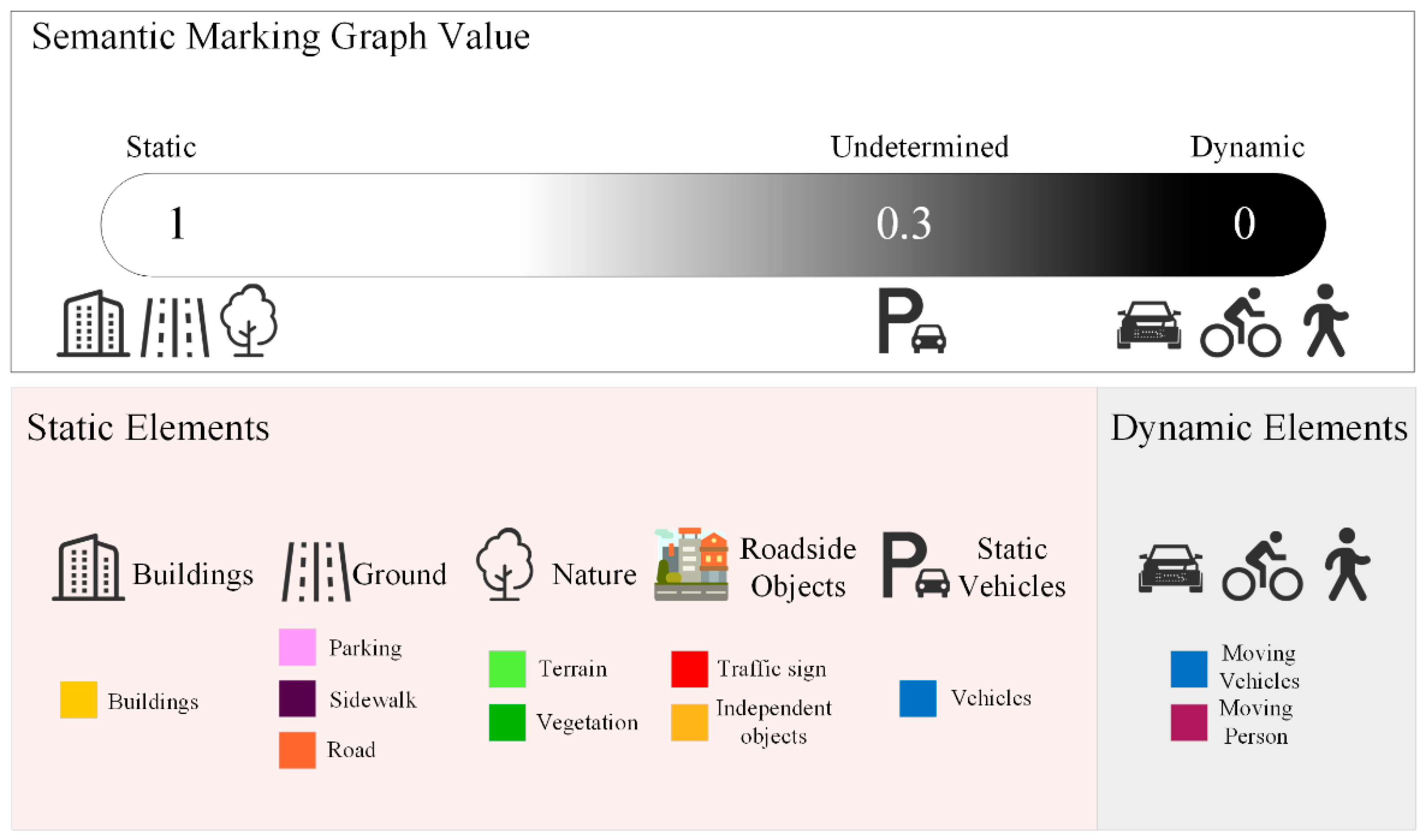
Figure 7.
Schematic diagram of environmental elements selection based on context information.

Figure 8.
Schematic diagram of frame-to-map ICP.

Figure 9.
Schematic diagram of weight matrix assignment.
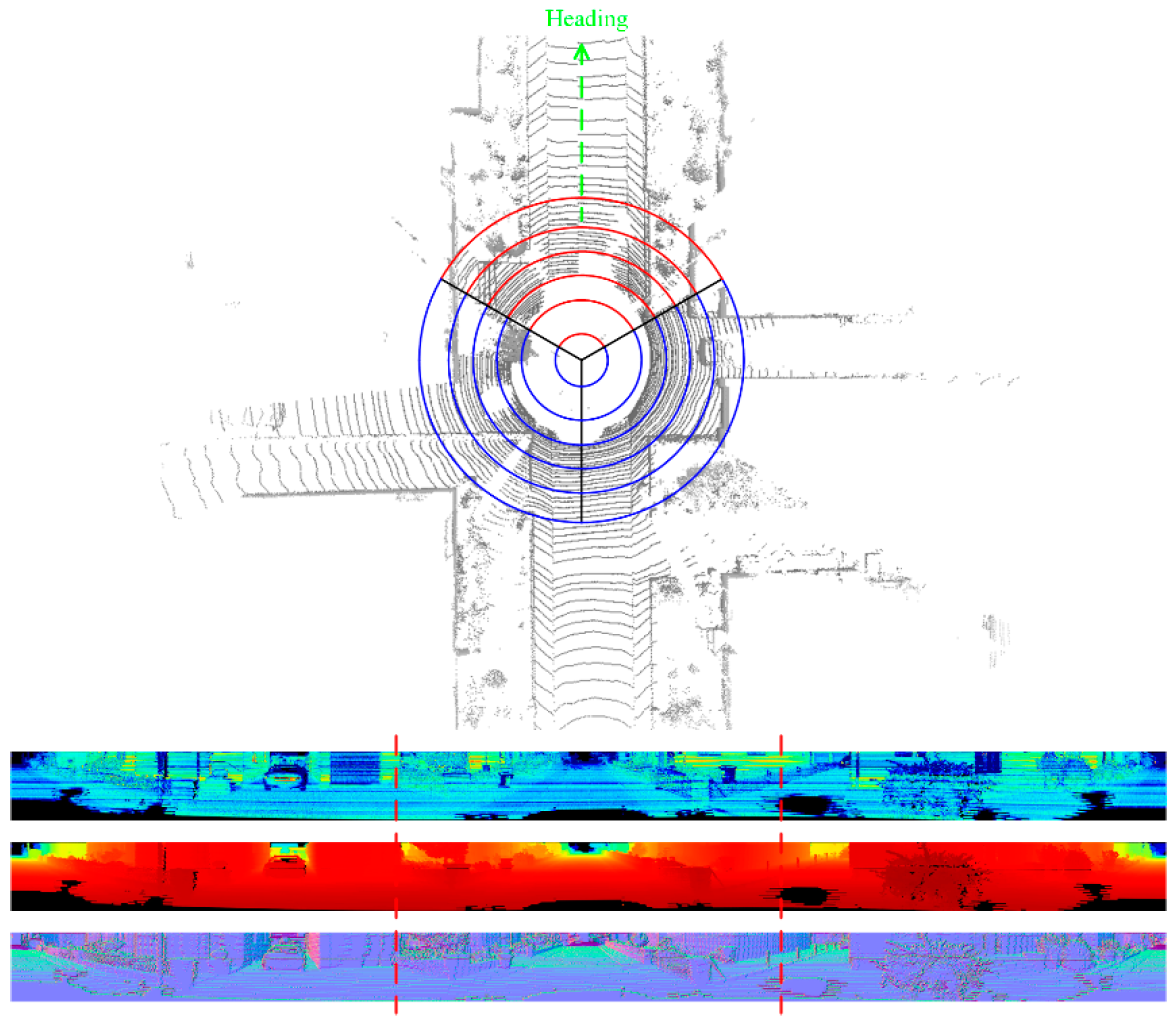
Figure 10.
Experimental results of KITTI dataset.


Figure 11.
The order of semantic maps is sequence 00 05 08.

Figure 12.
Experimental results of SemanticPOSS dataset.


Table 1.
Quantitative comparison of mIoU scores on SemanticKITTI test set (sequences 11–21) of each algorithm, SANet is the proposed method.
Table 1.
Quantitative comparison of mIoU scores on SemanticKITTI test set (sequences 11–21) of each algorithm, SANet is the proposed method.
| Method | Car | Bicycle | Motorcycle | Truck | Other-vehicle | Person | Bicyclist | Motorcyclist | Road | Parking | Sidewalk | Other-ground | Building | Fence | Vegetation | Trunk | Terrain | Pole | Traffic-sign | mIoU(%) |
|---|---|---|---|---|---|---|---|---|---|---|---|---|---|---|---|---|---|---|---|---|
| RangeNet | 91.4 | 25.7 | 34.4 | 25.7 | 23.0 | 38.3 | 38.8 | 4.8 | 91.8 | 65.0 | 75.2 | 27.8 | 87.4 | 58.6 | 80.5 | 55.1 | 64.6 | 47.9 | 55.9 | 52.2 |
| SquSegV3 | 92.5 | 38.7 | 36.5 | 29.6 | 33.0 | 45.6 | 46.2 | 20.1 | 91.7 | 63.4 | 74.8 | 26.4 | 89.0 | 59.4 | 82.0 | 58.7 | 65.4 | 49.6 | 58.9 | 55.9 |
| SalsaNet | 83.3 | 25.4 | 23.9 | 23.9 | 17.3 | 32.5 | 30.4 | 8.3 | 89.7 | 51.6 | 70.4 | 19.9 | 80.2 | 45.9 | 71.5 | 38.1 | 61.2 | 26.9 | 39.4 | 44.2 |
| SalsaNext | 90.9 | 36.4 | 29.5 | 21.7 | 19.9 | 52.0 | 52.7 | 16.0 | 90.9 | 58.1 | 74.0 | 27.8 | 87.9 | 58.2 | 81.8 | 61.7 | 66.3 | 51.7 | 58.0 | 54.5 |
| SANet | 92.5 | 49.7 | 37.9 | 38.7 | 32.4 | 57.5 | 52.0 | 33.5 | 91.4 | 64.0 | 75.1 | 28.8 | 88.6 | 59.6 | 81.0 | 62.5 | 65.4 | 53.2 | 61.6 | 59.2 |
Table 2.
Comparison of APE for translation part (Unit: m).
| Sequences | SuMa++ | DynaSLAM | DM-SLAM | Our Approach | |||
|---|---|---|---|---|---|---|---|
| RMSE | RMSE | RMSE | RMSE | Mean | Median | Std. | |
| 00 | 1.16 | 1.4 | 1.4 | 1.15 | 1.00 | 0.90 | 0.56 |
| 01 | 17.05 | 9.4 | 9.1 | 14.65 | 13.88 | 13.95 | 4.69 |
| 02 | 8.02 | 6.7 | 4.6 | 8.62 | 7.99 | 7.63 | 3.24 |
| 03 | 1.34 | 0.6 | 0.6 | 1.04 | 0.95 | 0.98 | 0.45 |
| 04 | 0.33 | 0.2 | 0.2 | 0.32 | 0.29 | 0.30 | 0.13 |
| 05 | 0.75 | 0.8 | 0.7 | 0.67 | 0.61 | 0.57 | 0.28 |
| 06 | 0.49 | 0.8 | 0.8 | 0.48 | 0.44 | 0.38 | 0.19 |
| 07 | 0.50 | 0.5 | 0.6 | 0.47 | 0.44 | 0.43 | 0.17 |
| 08 | 3.25 | 3.5 | 3.3 | 2.56 | 2.26 | 1.99 | 1.21 |
| 09 | 1.26 | 1.6 | 1.7 | 1.24 | 1.14 | 1.11 | 0.49 |
| 10 | 1.41 | 1.2 | 1.1 | 1.32 | 1.27 | 1.26 | 0.38 |
Table 3.
Comparison of datasets.
| Frames | Points | Type | Average Instances per Frame | |||
|---|---|---|---|---|---|---|
| People | Rider | Car | ||||
| Cityscapes | 24,998 | 52,425 M | images | 6.16 | 0.68 | 9.51 |
| KITTI | 14,999 | 1799 M | point clouds | 0.63 | 0.22 | 4.38 |
| SemanticPOSS | 2988 | 216 M | point clouds | 8.29 | 2.57 | 15.02 |
Table 4.
Absolute Pose Error (APE) for translation part (Unit: m).
| Sequences | Our Approach | |||
|---|---|---|---|---|
| RMSE | Mean | Median | Std. | |
| 00 | 0.09 | 0.08 | 0.08 | 0.03 |
| 01 | 0.16 | 0.15 | 0.13 | 0.07 |
| 02 | 0.13 | 0.10 | 0.06 | 0.08 |
| 03 | 0.10 | 0.10 | 0.09 | 0.04 |
| 04 | 0.13 | 0.11 | 0.10 | 0.06 |
| 05 | 0.17 | 0.16 | 0.15 | 0.07 |
Publisher’s Note: MDPI stays neutral with regard to jurisdictional claims in published maps and institutional affiliations. |
© 2021 by the authors. Licensee MDPI, Basel, Switzerland. This article is an open access article distributed under the terms and conditions of the Creative Commons Attribution (CC BY) license (https://creativecommons.org/licenses/by/4.0/).
Share and Cite
MDPI and ACS Style
Wang, W.; You, X.; Zhang, X.; Chen, L.; Zhang, L.; Liu, X. LiDAR-Based SLAM under Semantic Constraints in Dynamic Environments. Remote Sens. 2021, 13, 3651. https://0-doi-org.brum.beds.ac.uk/10.3390/rs13183651
AMA Style
Wang W, You X, Zhang X, Chen L, Zhang L, Liu X. LiDAR-Based SLAM under Semantic Constraints in Dynamic Environments. Remote Sensing. 2021; 13(18):3651. https://0-doi-org.brum.beds.ac.uk/10.3390/rs13183651
Chicago/Turabian StyleWang, Weiqi, Xiong You, Xin Zhang, Lingyu Chen, Lantian Zhang, and Xu Liu. 2021. "LiDAR-Based SLAM under Semantic Constraints in Dynamic Environments" Remote Sensing 13, no. 18: 3651. https://0-doi-org.brum.beds.ac.uk/10.3390/rs13183651
Note that from the first issue of 2016, this journal uses article numbers instead of page numbers. See further details here.