Article

Measurements and Modelling of Aritificial Sky Brightness: Combining Remote Sensing from Satellites and Ground-Based Observations

1
Department of Physics, Eszterházy Károly Catholic University, 3300 Eger, Hungary
2
Department of Physics, Eötvös Loránd University, BDPK, 9700 Szombathely, Hungary
3
Hungarian Meteorological Service, 1024 Budapest, Hungary
*
Author to whom correspondence should be addressed.
Remote Sens. 2021, 13(18), 3653; https://doi.org/10.3390/rs13183653
Submission received: 30 July 2021 / Revised: 31 August 2021 / Accepted: 7 September 2021 / Published: 13 September 2021
(This article belongs to the Special Issue Light Pollution Monitoring Using Remote Sensing Data)

Abstract

:
In recent decades, considerable research has been carried out both in measuring and modelling the brightness of the sky. Modelling is highly complex, as the properties of light emission (spatial and spectral distribution) are generally unknown, and the physical state of the atmosphere cannot be determined independently. The existing radiation transfer models lack the focus on light pollution and model only a narrow spectral range or do not consider realistic atmospheric circumstances. In this paper, we introduce a new Monte Carlo simulation for modelling light pollution, including the optical density of the atmosphere and multiple photon scattering, then we attempt to combine the available information of satellite and ground-based measurements to check the extent to which it is possible to verify our model. It is demonstrated that we need all the separate pieces of information to interpret the observations adequately.

1. Introduction

1.1. Ground Measurements of ALAN

The measurement of artificial light at night (ALAN) has several decade-long history. During this time, different measurement methods and types of equipment were used. These are single-channel measurement devices, such as Sky Quality Meters (SQM), or multi-channel devices, like digital single-lens reflex (DSLR) cameras and mirrorless cameras (MILC).
The SQM (e.g., [1]) devices measure the zenith brightness and are widely used, but have some drawbacks compared to multi-channel methods. They contain a custom filter that does not exactly match any astronomical or photopic band, but has an extra sensitivity at blue wavelengths. The displayed value measured by the instrument often uses a unit of measurement where the reference is a stellar spectrum, which has different values at different wavelengths. Thus it does not correspond to the astronomically accepted definition of magnitude [2].
For multi-channel measurements, DSLR and MILC cameras are used to monitor the quality of the night sky and light pollution [3]. These cameras save images in raw format and can be calibrated to measure the radiance of the sky. The distribution of sky brightness can be represented by using false colour images, being a good method for comparative analysis [4,5,6,7,8,9,10]. With these cameras, the goal is to provide all-sky measurements. This task can be performed either by applying fish-eye lenses or taking several images of the full sky and stitching them together to create a full-sky panorama image. Fish-eye lenses often lack the resolution and precision close to the horizon, which is normally the most interesting for light pollution measurements. This problem can be solved by taking two or multiple fish-eye images in the vertical plane [11], but in return, the resolution of the zenith becomes poorer.
To achieve the highest accuracy and resolution in dark places, it is recommended to take a large panorama of several photos from different directions. Kolláth et al. [2] use a solution that covers the whole sky by using a full-frame digital camera mounted on a robotic panoramic head with a 24 mm or 35 mm linear lens. The method does not require a long exposure time so that the apparent movement of stars and the sky does not cause any artificial distortion during the measurement. It is also possible to correct the acquired images afterwards based on astrometry [2].
Light pollution is most often characterised by measuring the sky brightness. Galatanu et al. [12] present a supplementary method for describing the extent of light pollution based on global measurements or statistical tests, an approach based on direct imaging of both light sources and the light pollution they cause. These are differential imaging measurements that provide a quantitative estimate of light pollution levels in target areas (e.g., building facades) by determining the luminous flux that represents the actual light pollution. In addition to the existing measurements, their studies use an alternative measurement method, which aims to measure the amount of light reaching the building facade and then directly study the sources of light pollution, which form the missing link in the causal system.

1.2. Satellite Measurements of ALAN

Obtaining information about the emission spectrum of outdoor artificial light sources on large spatial scales is challenging. Ground measurements with DSLR and MILC cameras are suitable for spectral analysis but are very localized. The majority of remote-sensed nighttime lighting data is monochrome, obtaining data in a single channel with a broadband filter. Today, it is very interesting to measure the night lighting spectrum on a large scale since rapid changes are currently taking place [13,14,15]. For several decades, outdoor lighting has mainly used high-pressure sodium (HPS), low-pressure sodium (LPS), metal halide (MH) and fluorescent lamps. Recently, however, there has been a widespread transition to white light-emitting diode (LED) lamps, which are now becoming the dominant source and whose emissions have been associated with more severe environmental impacts [16,17,18].
The Suomi NPP (National Polar-orbiting Operational Environmental Satellite System Preparatory Project) is one of the most comprehensive satellite remote sensing systems for measuring the brightness of the Earth’s surface. The satellite orbits in a polar sun-synchronous orbit at an altitude of 824 km above the surface. Its specialised Visible Infrared Imager Radiometer Suite (VIIRS) takes images of the surface of our planet in the visible and infrared range. However, due to the limited field of view of VIIRS, it cannot see the whole Earth at once. A global scan can be performed as follows: when it passes over the equator from south to north, it always passes over the equator at the same time but at different longitudes as the Earth passes beneath it. In this way, it can photograph the entire surface of the Earth in a single day. Since the bands in its field of view are pritty broad (3000 km), there is an overlap between the images taken at adjacent passes, even at the equator. The VIIRS DNB (Day/Night Band) night images are often analyzed for a longer time period to get current data of nighttime lights [19]. These images are affected by a number of factors, including atmospheric conditions, moonlight, snow and clouds [19,20,21]. Hence, the data quality is not good enough to detect temporal variations. Due to the anisotropic reflection characteristics of the Earth, the surface is modelled with a bidirectional reflection distribution, and the direction of solar radiation and satellite viewing changes the satellite-observed radiation reaching the surface. Because of this, for obtaining accurate brightness data, the measurements need to be corrected.
Besides the actual remote-sensing of satellites, an alternative source of spatial and temporal data on the spectrum of artificial night lighting is the photographs taken by astronauts on the International Space Station (ISS). The obtained imagery can be used to estimate the spectral type of ground light sources based on colour information [22].
Bouroussis and Topalis [23] offer an alternative to ground-based measurements applying unmanned drone aircrafts measuring light pollution. Their aim is to develop a new standardised method for light pollution measurement that uses a variety of lighting bodies measured by unmanned aircraft systems. This technology uses drone aircraft equipped with multiple types of sensors, programmed to fly over predefined areas and routes and to perform complex measurements with limited human intervention. In contrast to ground-based measurements, this technology allows fast, simple, accurate and repeatable measurements from multiple angular positions and altitudes. It offers new ways to investigate and detect problems related to light pollution and intrusive lighting, for which there are currently few standardised computational and measurement methods. Measurements with unmanned drone aircraft allow a holistic, three-dimensional assessment of lighting.
In this paper we use the 2019 VIIRS DNB data (see [19]), especially the VNL V2 annual averages (https://eogdata.mines.edu/nighttime_light/annual/v20/, accessed 28 May 2021).

1.3. Modelling of ALAN

Ground and satellite measurements cannot provide a satisfactory amount and quality data for creating light pollution maps. Ground measurements can be well-calibrated, and spectral data gain is possible but is localised. Satellite measurements are often monochrome and require further corrections to get comparable data with other measurement methods. For comprehensive maps, modelling is an essential method that uses data from sky brightness databases for certain locations, and from these, the missing data can be extrapolated. One example that aims to model natural sky brightness is the GAMBONS (GAia Map of the Brightness Of the Natural Sky) model that maps the night brightness of the sky in cloudless and moonless nights. GAMBONS is based on the extra atmospheric star radiance data obtained from the Gaia and Hipparcos catalogue. These contain astrometric and photometric information for more than 1.6 billion stars. Besides the star radiance, zodiacal light and airglow is taken into account to estimate effects of atmospheric attenuation and scattering [24].
Some previous radiative transfer models were developed to model the atmospheric conditions and not the light pollution directly. Moncet et al. [25] present a fast and accurate method for numerical modelling of band transmissions during radiative transfer in media with inhomogeneous thermodynamic properties, involving a mixture of absorbing gases with varying concentrations. The Optimal Spectral Sampling (OSS) method was primarily designed for modelling radiance values measured by sounding radiometers in the infrared range and has been extended to the microwave range but can also be applied in the visible and ultraviolet spectrum. The OSS allows the use of remote sensing and satellite measurements and includes the data of observations into numerical weather prediction models. The method is based on an extension of the exponential sum fitting transmittance technique by obtaining the channel-averaged radiative transfer from the weighted sum of monochromatic calculations. OSS is essentially a monochromatic method that allows accurate treatment of surface reflectance and the spectral variations of the Planck function. The model takes into account the variation of the surface emissivity within the channel transmission band by a function. In addition, the method can be easily coupled with multiple scattering calculations, an important factor when modelling radiance in cloudy weather. The OSS method can be directly applied to interferometric measurements. It enables the selection of numerical accuracy relative to a reference line-by-line model, which allows optimising accuracy and computational speed for a given application. In general, only a few monochromatic points are needed to model channel radiations with a brightness temperature accuracy of a few hundredths of K.
Another method, that was designed for modelling atmospheric conditions and multilayered clouds, was described by Wang et al. [26] who developed a fast and flexible model for simulating thermal infrared radiation transfer in scattering-absorbing atmospheres. The model can simulate radiation transfer in a single run, taking different user-defined viewing angles and fluxes into account. Furthermore, the model considers complex and realistic cases such as the coexistence of ice clouds, water clouds and mineral dust layers within an atmospheric column. In the model, for an atmosphere with three scattering layers (water, ice and mineral dust), the root mean square error of the simulated brightness temperatures at the top of the atmosphere is approximately 0.05 K. The relative flux errors at the boundary and interior levels are below 1%. Due to its computational efficiency and accuracy, the model can facilitate radiative transfer simulations based on remote sensing measurements of high spectral resolution and narrowband infrared measurements, as well as weather forecasting applications processing large amounts of data. The chosen spectral resolution of 0.1 cm 1 prevents the extension of their current model to highly absorptive bands (e.g., 600–700 cm 1 ). However, replacing the applied clear sky module with a higher performance model may be suitable for applications involving spectral bands with strong absorption.
A recent study [27] describes a spectral data compression (SDCOMP) radiative transfer model in which satellite and ground-based high spectral resolution measurements are taken into account to create an accurate and efficient radiative transfer model for weather and climate applications, for atmospheric measurements. The model is capable of simulating radiation values in the visible and infrared spectral regions. The SDCOMP approach ‘compresses’ the optical properties of spectral data and radiance domains and then applies a two-fold principal component analysis (PCA) to reduce the computational load. The two-fold principal component analysis includes a PCA based on optical properties for a given atmospheric scenario and then a radiation-based PCA from a large number of atmospheric scenarios derived from a precomputed radiation data set. The former is useful for simulating radiations with relatively low spectral resolutions at a few representative wavelengths, while the latter is performed at all wavelengths to obtain results with the desired spectral resolution. The procedure ensures that each monochromatic radiative transfer calculation can be performed time-efficiently, and the number of such calculations can be optimised. SDCOMP is about three orders of magnitude faster than numerical radiative transfer calculations.
In a most recent paper Kyba et al. [28] emphasize that studying night lights from multiple angles of view provides additional information that can be used to improve the results of current night-light-based remote sensing and to make corrections to models that simulate artificial skyglow. One of the most physically detailed artificial night sky brightness models is the Illumina model [29], which has been under continuous development since 2005 and includes a cloud cover scheme, a blocking scheme for subgrid obstacles (trees and buildings), and a full hyperspectral modelling approach. However, these methods do not realistically account for the geographical variability of obstacle properties. Direct measurement of upward light emission using multi-angle imagery is a critical factor to improve model accuracy [28].
The above models show solutions for radiative transfer computation, however, most of them are not specific for light pollution rather than for atmospheric or meteorological predictions. Some of them models only a narrow range of the radiation spectrum (e.g., infrared) or focus only on atmospheric conditions relevant to meteorology. The total sky radiance is highly influenced by multiple photon scattering, the proper quantification of which is still a challenging task. Kocifaj [30] describes a numerical model that gives the relative contribution of higher-scattering radiances to the total sky radiance, treated analytically for all orders of scattering. The method utilizes the same processor time for each scattering mode, thus it allows for rapid estimation of higher-scattering radiances and residual error. The effects of multiple scattering become important when the light source is at a higher distance than 30 km.
Monte Carlo simulation has been recently used as a powerful tool for numerical modelling of radiation processes and radiation transfer, which allows to efficiently model the relationship between the physical properties of an object and the radiation it emits. The method must take into account the adverse consequences of Monte Carlo noise in the simulation results. This noise can be reduced, e.g., by corrective measurements [31]. Using a similar concept, in this paper, we show a new model of light pollution based on Monte Carlo simulation of multiple photon scattering. The model is corrected with the data of ground measurements at known locations, based on which the brightness distribution can be calculated for custom locations.

2. Materials and Methods

2.1. Measurements

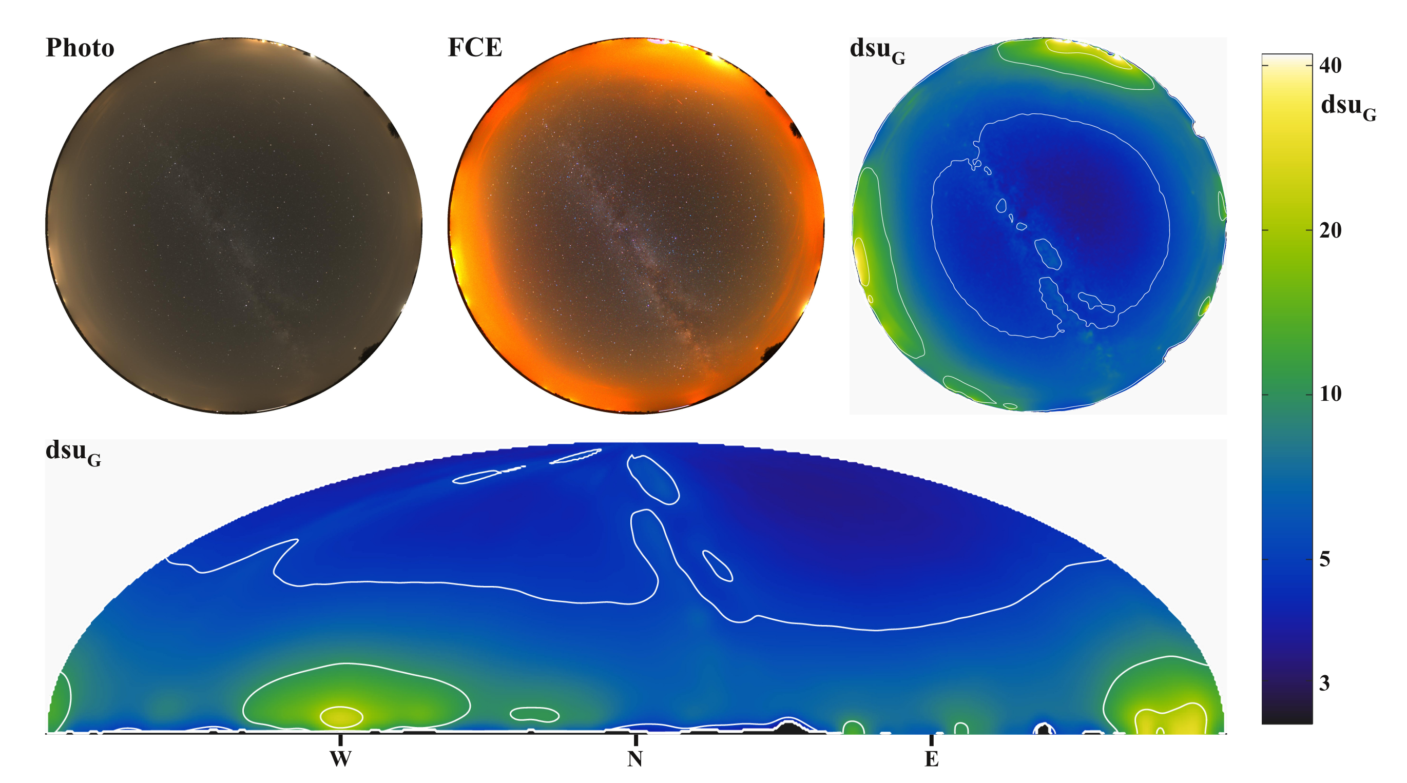
2.1.1. DiCaLum: All Sky Radiance Measurements

The simple instruments commonly used (e.g., Unihedron Sky Quality Meter) are essentially illuminance meters. Still, they have a limited field of view and are calibrated to give a part of the sky’s average radiance (approximately luminance). These instruments proved helpful, especially in the early days, and they are still significant in sky quality determination. However, they only provide information on a small part of the sky, and their spectral sensitivity is different from that of all other instruments. With the development of digital cameras, it has become possible to make more precise but often at lower temporal resolution measurements with cameras equipped with fish-eye optics of appropriate quality [1,3]. Image radiance measurements have opened a new way of determining sky quality. A significant flaw that remains with fish-eye systems is that near the horizon, where the sky is more illuminated by the dome of light from settlements, the lens’s vignetting effect is most vital, making measurements uncertain.
To overcome these problems, we have developed our mobile laboratory, where instead of using fish-eye optics, we create a mosaic of multiple images. In the commonly used setup, a 24 mm focal length optic is used to take 28 pictures. Since manually taking this many photos is problematic, we use a robotic panoramic head to move the camera. Under standard conditions, a 6-second exposure is sufficient for darker locations (ISO 6400 and f/1.4 brightness) so that a high-resolution sky map can be taken in 10 min with the equipment set up at a given area.
The measurements are represented in dark sky unit (dsu) [2] for the R, G and B bands of the camera. It is a mean spectral radiance weighted by the spectral response of the camera filters. 1 dsu is equivalent to 1 nW/m 2 /sr/nm. The radiance map can be converted to different projections. We use standard equal zenith angle fish-eye projection or Hammer-Aitoff equal-area projection in this paper (see Figure 1).
A Konica-Minolta 2000A spectroradiometer complements the portable laboratory, and the primary purpose is to calibrate digital cameras. However, the instrument is sensitive enough to measure the spectral radiance of the sky under natural conditions (as low as 2 nW/m 2 /sr/nm depending on the spectral range). The possibility of the parallel camera and spectroradiometer measurements further increases the accuracy of the measurements.

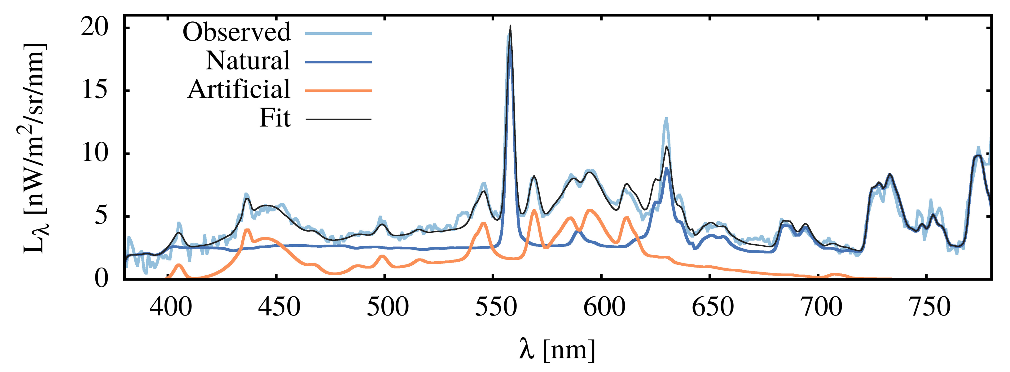
2.1.2. Fitting the Natural Spectrum Components

For spectral measurements, we used the already mentioned Konica-Minolta CS2000A spektroradiometer. To achieve the highest sensitivity, we use the widest field of view of 1 . The bandwidth of the device is FWHM = 3.9 nm at 550 nm based on our measurements. All the synthetic spectra used in this paper is calculated with the same bandwidth. The reported sensitivity of the device is L = 0.005 cd/m 2 at the longest measurement time (241 s) The colour of the night sky carries crucial information, essentially a fingerprint of the composition of light. The natural and artificial spectra of the sky are very different, so the components are separable. This makes it possible to determine the radiance of the natural component in a light-contaminated sky. This is important because this component is constantly changing due to natural processes. The natural component determined from the spectrum is then used as a model for imaging measurements of the whole sky.
A typical spectrum and its decomposition are shown in Figure 2. The artificial component is fitted with the spectra of CFL, sodium lamp and LED typically used in Hungary. The natural part was based on the “Advanced Cerro Paranal Sky Model” (https://www.eso.org/sci/software/pipelines/skytools/skymodel, accessed 1 June 2020) [32]. In the SkyCalc web interface, we set the convolving line spread function to a Gaussian matching the bandwidth of the Konica-Minolta CS2000A spectroradiometer. However, we do not use these spectra directly but the decomposition to the different spectral components (e.g., the main oxygen, sodium lines, OH bands, and the continuous parts). All the spectral components are fitted independently. Thus the method provides an independent fit from the Cerro Paranal Sky Model.
The natural component from the sky spectrum can be used to select the best fitting natural sky model (e.g., GAMBONS-https://gambons.fqa.ub.edu/, accessed 28 May 2021). Figure 3 displays the natural sky luminance (without the stars and the Milky Way) as a function of altitude. The models are provided for two different solar activity levels and for AOD = 0.05, 0.10, 0.20, 0.30 and 0.40 (from top to bottom). The values for the black dots are calculated from the decomposed spectroradiometer data. This comparison confirms the good transparency at the given night. The fit gives the natural component estimate and an important input for model parameters (e.g., AOD).

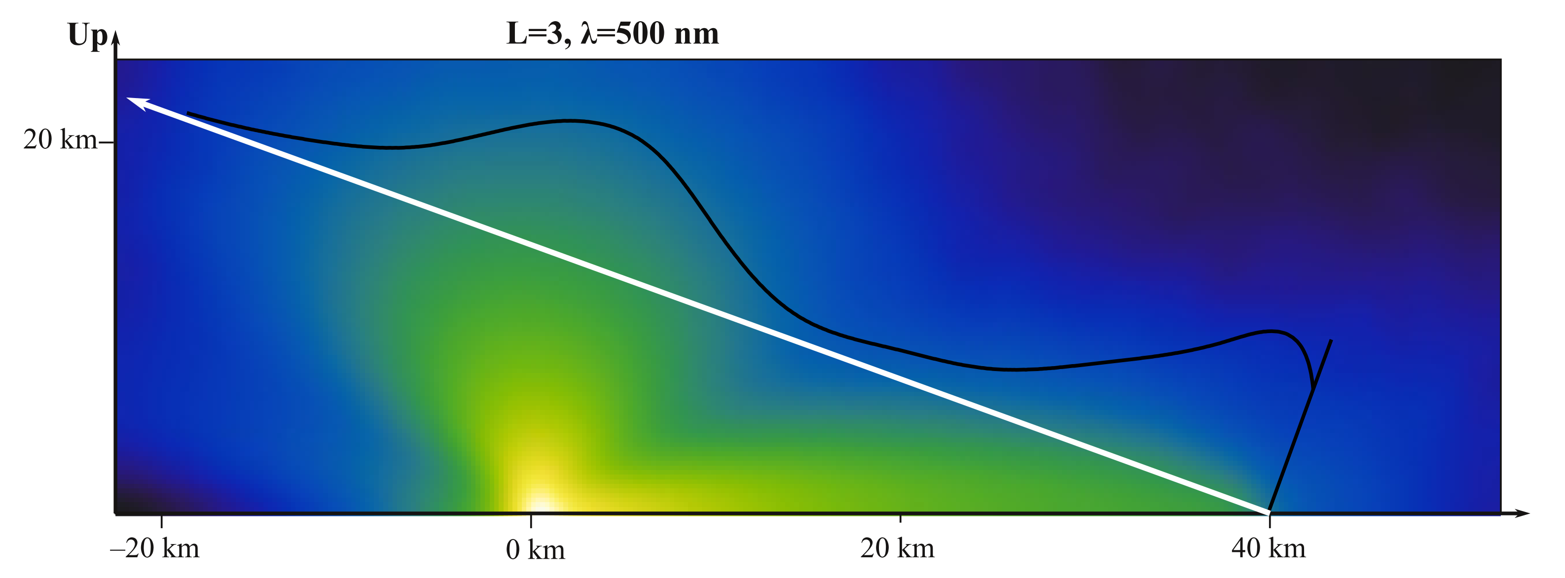
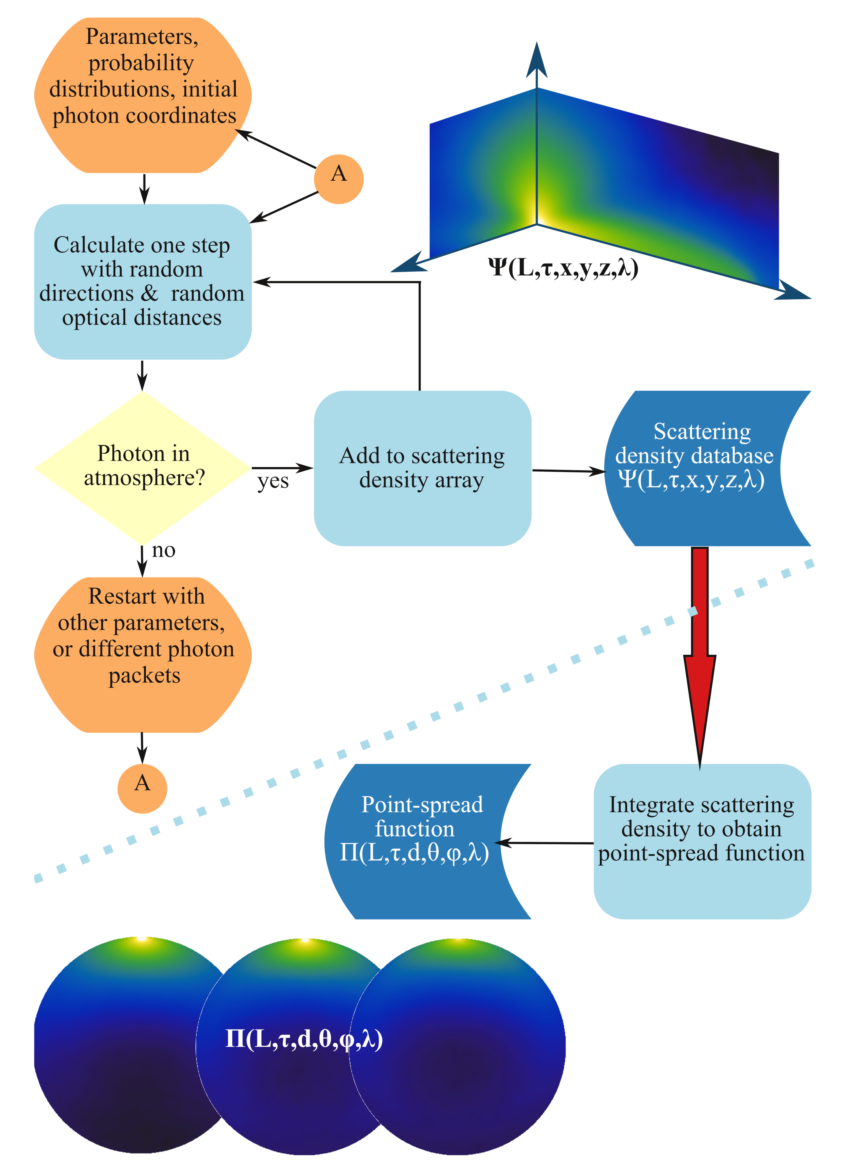
2.2. ScatDenMC: A Scattering Density Monte Carlo Radiation Transfer Model

Light pollution modelling is essentially a radiative transfer problem. The difficulty is to treat the atmospheric scattering with sufficient accuracy. The problem can only be solved numerically, which can be done in two ways: either by solving the integrodifferential equations of radiative transfer by computer or by Monte-Carlo simulation with the accurate treatment of the elementary scattering processes. We have chosen the latter since it requires fewer approximations. The Monte Carlo method has the disadvantage of being more computationally demanding, but in many cases, the increased accuracy (e.g., multiple scattering) compensates for this.
The first Monte Carlo radiative transfer calculation step is to distribute random photon packets to the atmosphere. Since our goal is to create a point spread function, we use a point source in the calculations.
Spherical harmonics can reasonably approximate the directional distribution of the source. In the case of axis symmetry, it is usually sufficient to calculate the emission corresponding to the first 4–5 Legendre polynomials (L = 0, ...,4). Note that L = 0 corresponds to the same probability of light leaving in all directions (spherical symmetry), and L = 1 gives the Lambertian distribution. Higher-order polynomials do not directly relate to actual sources; we use them to fit a polynomial series to real word distributions.
Monte Carlo simulation provides an optimal method for modelling sky brightness. In its simplest form, this method is relatively straightforward: It generates photon scattering using random numbers, and then in the next step, using only random numbers again, it determines the length of the path of the next scattering event. The following random number determines the new direction of the photon after scattering. Then the cycle starts again until the packet leaves the atmosphere, is absorbed, or reaches the detector. This procedure defines the simplest Monte Carlo modelling, a brute force method that is computationally inefficient. The main reason for the poor performance is that most of the photons never reach the detector.
The real improvement in numerical efficiency is the use of peel-off methods [33]. The technique works in the same way as brute-force modelling, but in this case, the weight of the photon packet potentially reaching the virtual camera is calculated based on each scattering event. From the scattering phase function, we can calculate the probability that the photon will propagate after the scattering event in the direction of the detector. The forced photon arrivals are weighted by the distance and optical depth between the scattering point and the observer. In theory, this method gives the same results as the standard method. The drawback of the peeling method is that low probability scatterings (which occur only rarely in the simulation) can be given considerable weight in some situations. If these events infrequently happen (in a statistically low number), the Monte Carlo simulation statistics are flawed, leading to noisy results.
The peel-off method can be further improved in terms of noise statistics and optimized CPU time. We developed a numerical method, the scattering density Monte Carlo radiative transfer code (ScatDenMC). Based on the scattering events, a spatial probability density distribution can be generated, which gives the probability of a photon leaving a given spatial point in a given direction.
The scattering density is calculated in a discrete Cartesian grid. After each scattering event, the code calculates the increment to the given volume element in the grid. In general, in each grid point, a 2D function gives the directional distribution of the scattering probability. We do not store the mean phase function for all the directions to reduce data storage, only for a finite number of observer locations. Thus the scattering density has the following form:
Ψ ( L , AOD , o k , x j , y j , z j , λ ) = m P ( μ j ) e ( τ k j ) W m ,
where x j , y j , and z j are the coordinates of the jth grid point, L is the Legendre polynomial order, AOD gives the aerosol opical depth of the atmosphere, o k represents the coordinates of the kth observer location, λ is the wavelength, and W m is the weight of the photon packet at the mth scattering event. The weight of the photon packet is set initially to 1, and it is decreased after ground reflection and atmospheric absorption.
The above process is repeated with photon packets of different wavelengths. Since the results smoothly depend on the wavelength, it is sufficient to calculate, e.g., 20 nm steps, which results in 21 different distributions over the whole visible range.
Figure 4 displays the sections of the scattering density distributions for the vertical plane, including the observer and the source. This density function is calculated from the observer’s point of view, including the distortion due to the scattering phase function and the weight determined by the optical depth between the observer and the given grid point. This interaction results in the skewed structure of the distribution.
In the above formalism we mentioned only the main parameters of the model: L and AOD. However, there are additional parameters. The scale height of the aerosols is fixed to 2.2 km in this paper, the shape of the aerosol profile is the standard exponential one. However, it is straightforward to include additional profiles in the model. For a given parameter set, the scattering density distribution depends on the location ( x j , y j , z j ), wavelength λ and direction Thus this is, in reality, a 6-dimensional distribution. It is convenient to reduce the number of dimensions for internal data storage. The different λ values can be handled separately, and the directional distribution is reduced to a few observers locations. Thus only a 3D discrete spatial distribution is stored according to the direction of a finite observation point (virtual camera).
It is also possible to treat the 3D discrete density function with an appropriate smoothing algorithm (e.g., low-frequency filtering) to further reduce noise. The 3D continuous density function can then be obtained by interpolation.
After the Monte Carlo run, the density distribution is weighted according to the light absorption between the scattering point and the observer. For a given relative position of light emission and observer, this yields a 3D distribution function from which the sky radiances measured in the given direction can be obtained by taking integrals along the lines from the observer, which define the point spread function Π :
Π ( L , AOD , o k , θ , ϕ , λ ) = Ψ ¯ ( L , AOD , o k , x ( θ , ϕ , R ) , y ( θ , ϕ , R , z ( θ , ϕ , R ) , λ ) d R
Here we note the spatially interpolated density function by Ψ ¯ . The grid is dense enough to use a smoothing interpolation reducing the numerical noise of the Monte Carlo method. The integral is calculated along a line from the kth observer’s location to the direction represented by the horizontal polar coordinates: azimuth ( θ ) and elevation ( ϕ ) (see Figure 4)
Figure 5 displays the above procedure on a flowchart. There are two separate steps in the process, the first one generates the scattering density function ( Ψ ) and the second step interpolates and integrate the distribution along the different directions to get the point-spread function ( Π ). The two sub-processes are separated by the dotted blue line in the flowchart.
The model calculates the number of scattering events in the volume elements of the atmosphere. The density function depends on the relative location of the source and the observer—it makes the particular shape of the distribution. Figure 6 displays the dependence of the distribution on wavelength and the source emission function represented by Legendre polynomials. In the above figure, the source is at −30 km, and the observer is at 50 km). The results depend on many parameters: aerosol optical depth (AOD), density profile, humidity, the shape of the aerosol and Rayleigh scattering phase function, ground albedo, and the wavelength dependence of all these parameters.
In addition to the above representation of the scattering density ditribution, it is possible to average the scattering phase function of the photons at a given spatial point so that the average phase function can be obtained at some points.
Data storage was optimised by dividing the possible distances between the observer and the source into groups. We store the distribution function at six different distances in one run, which we repeat for six different ranges. As the distance increases, the spatial resolution can be reduced without loss of interpolation. This has the advantage that the increased cell volume compensates for the decreasing number of scattering events with increasing distance. With this method, the distribution function is well interpolated up to a distance of 300 km. Given the distance intervals, the Legendre polynomials and the different wavelengths, it is thus necessary to run the code several hundred different parameter combinations (for the above parameters). This also indicates that the system can be efficiently run optimised with a separate procedure on multi-thread computers capable of parallel runs. We are working with 1 billion photon bundles in a single run, so the total number of photon packets is in the order of 10 13 .
Once the scattering density is computed for all spherical harmonics, distance intervals and wavelengths, then for arbitrary spatial, directional and spectral distributions of sources, a simple algebra can be used to compute, for example, the sky brightness distribution at a given spatial location. All that is needed is weighted summation and convolution.
In the first step, the spectral distribution of the source is used to determine the spatial density function corresponding to the spectral response function of the detector. In a second step, the effect of the spatial emission distribution of the source is determined by the radiance distribution of the sky. Finally, the impact of each source is summed.
One important advantage of the Monte Carlo simulation is that higher-order scattering can be implemented with no additional effort. The running time decreased in the higher-order scattering steps since the number of photons decreases as the photon packets leave the atmosphere or lose weight after ground reflection. We performed a simple test on the importance of higher-order scattering. Models with AOD = 0.05, 0.2 and 0.3 were calculated with single, double or multiple (up to 8 steps) scattering order. Figure 7 displays the results. To simulate a real life scenario, the natural component of sky radiance is downloaded from the GAMBONS calculator for the same AOD values. We selected a date where the Milky Way is at low elevation. The simulation location and other parameters are given in the next section, for this test they have no relevance.
The figure clearly demonstrates the importance of higher order scattering. There is a significant increase in sky luminance from second order to high-order scattering. As expected, the difference increases with increasing aerosol optical depth. At AOD = 0.3, the zenith radiance increases by 20% from double scattering to multiple scattering. It means that models with double scattering underestimate sky brightness by 0.2 mpsas.
It is noted that the disadvantage of the current realisation of the procedure is that the topography can only be taken into account with limited accuracy. However, a significant advantage of the method over other methods is that it correctly handles the phenomenon of multiple scattering even in dense optical media (high AOD, clouds).

3. Results

Figure 8 summarises the proposed procedure to fit the models to the observational data. The inputs for the process are the spectrum of the sky in the zenith and at a couple of different elevations, the satellite database, the selected natural sky model from GAMBONS. In an optimal situation, the spectra of a representative sample of the sources are also available.
To test the fit of the models and observations, we chose the Hortobágy Starry Sky Park (inside Hortobágy National Park) in Hungary. The national park is located in the Great Hungarian Plain. There are no mountains within a radius of 60 km of the chosen observation point, and the terrain is flat for at least a distance of 200 km in several directions. The lack of mountains significantly simplifies data interpretation and modelling. The location of the observation is at coordinates 47.5754 N–21.2432 E. Measurements were taken twice: the first time on 2 September 2019 at 22:30 UT and the second time on 10 May 2021. On the first occasion, the transparency was not good, but the sky was clear. The estimated AOD was between 0.2 and 0.3. On the second occasion, we measured sky radiance with significantly better transparency. On this occasion, a comparison of spectroradiometric measurements with the GAMBONS model gives AOD = 0.05.

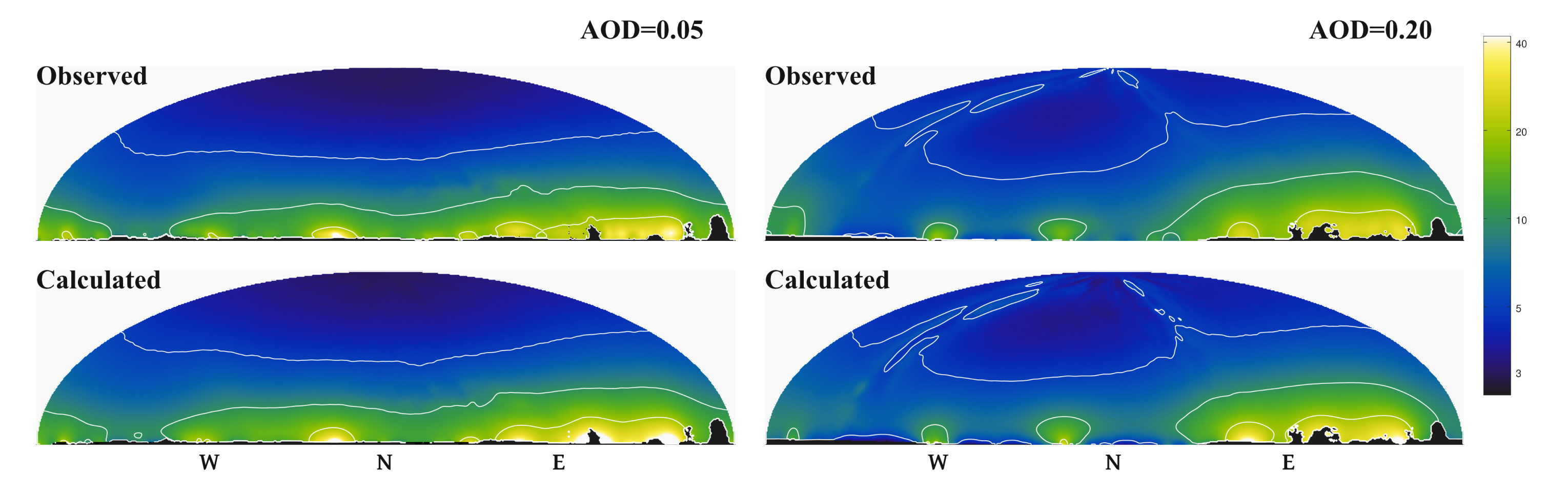
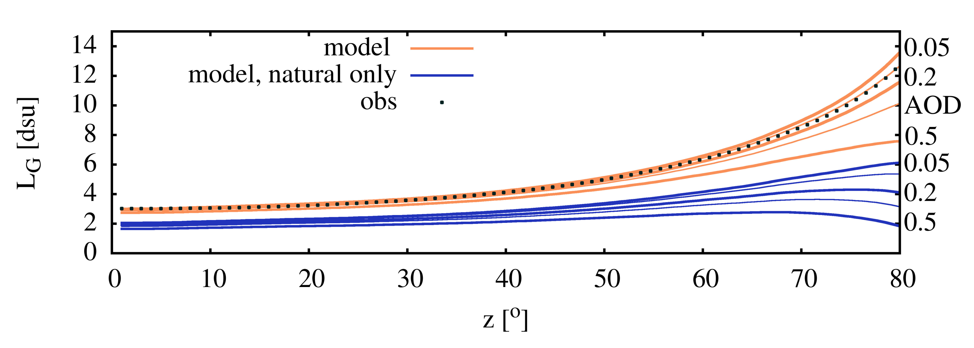
3.1. The Overall Fit of the Observations

To set the general parameters of the models, first, we averaged the measurements for different zenith angles, and then we compared it with the same curve calculated from the models. Figure 9 displays the mean radiance as a function of zenith angle both for the models and the observations. We plotted the model curves for different distance limits to check how the model converges as we include more and more sources with increasing distance.
At this stage, we fixed some of the parameters. We used the same spectral distribution for all the sources, which is typical for the mixture of lightings: sodium lamp (40%), compact fluorescent lamp (40%) and white LED (20%). We plan to perform a spectral survey in the neighbourhood of the measurements, which will make it possible to refine the spectral distribution of the settlements. The scale height of the atmospheric aerosols is fixed to h = 2 km.
For this study, we fixed the angular distribution of the source emission to the mixture of the first two Legendre polynomials. The fits with different combinations of the polynomials do not differ significantly if we allow the variation of the power output of the sources.
The fact that we measured the sky radiance at two substantially different atmospheric conditions (AOD = 0.05 and AOD = 0.20) provides an excellent opportunity to compare models with observations and to study the impact of AOD on sky quality. All parameters were assumed to be identical in the modelling, except for AOD. Although it is a strong assumption, the other parameters at this stage of our study provide reliable results. The changes due to the variation of ground albedo, aerosol scale height are significantly lower than caused by the changes in AOD. If the quality of the fit is suitable for both cases, the reliability of the comparison is enhanced.
Figure 10 compares the observed (top) and modelled (bottom) sky brightness of Hortobágy Starry Sky Park in Hungary, measured with a Sony ILCE 7SII camera equipped with a Samyang 24 mm lens. The sky brightness is visualized with false colours, and the contour lines refer to the same intensity value in the modelled and measured images, respectively. Because there are objects (trees and buildings) in the screen which obscures the sky, we used the measurement images to create a mask that achieves a similar effect in the modelled images. Masking helps in visual comparison. The brightness caused by artificial light sources together with the natural component shows a good fit to the observations. We used the observed images to create a mask since there are some obscuring objects (trees and buildings). The dependence of global structure on the sky radiance map on aerosol optical depts is well recovered by the models.

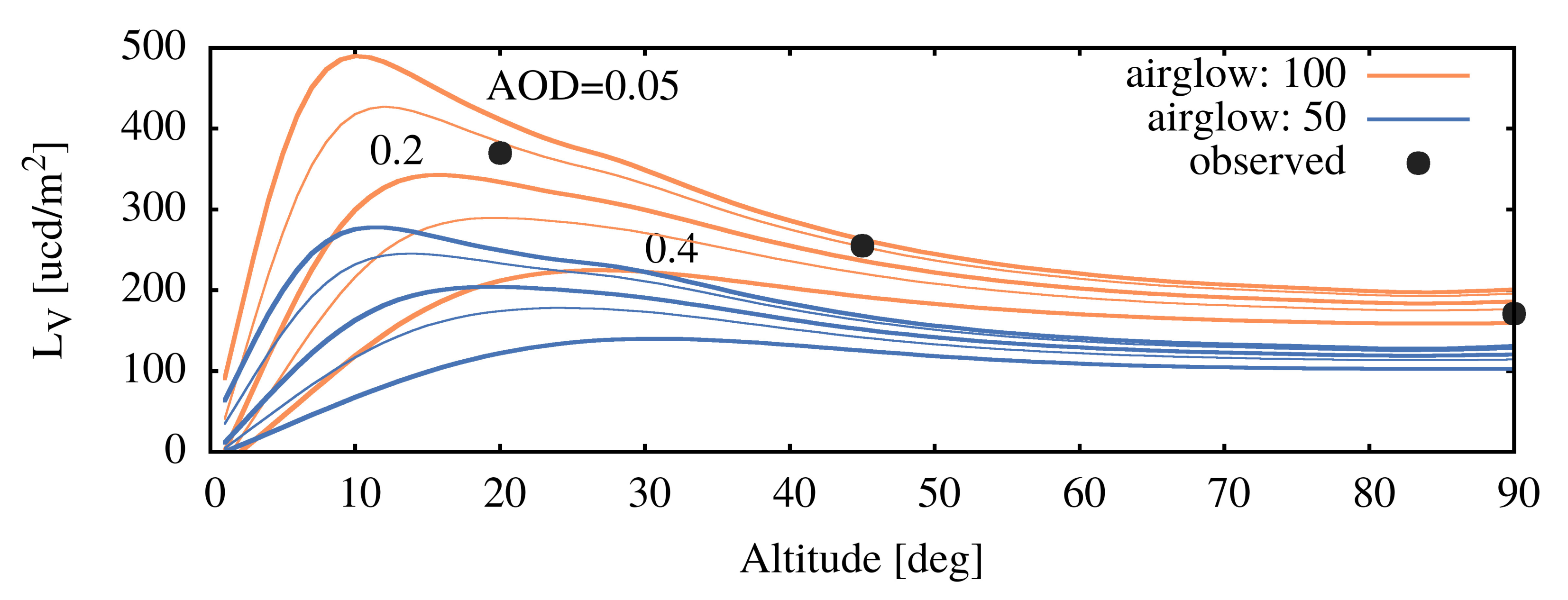
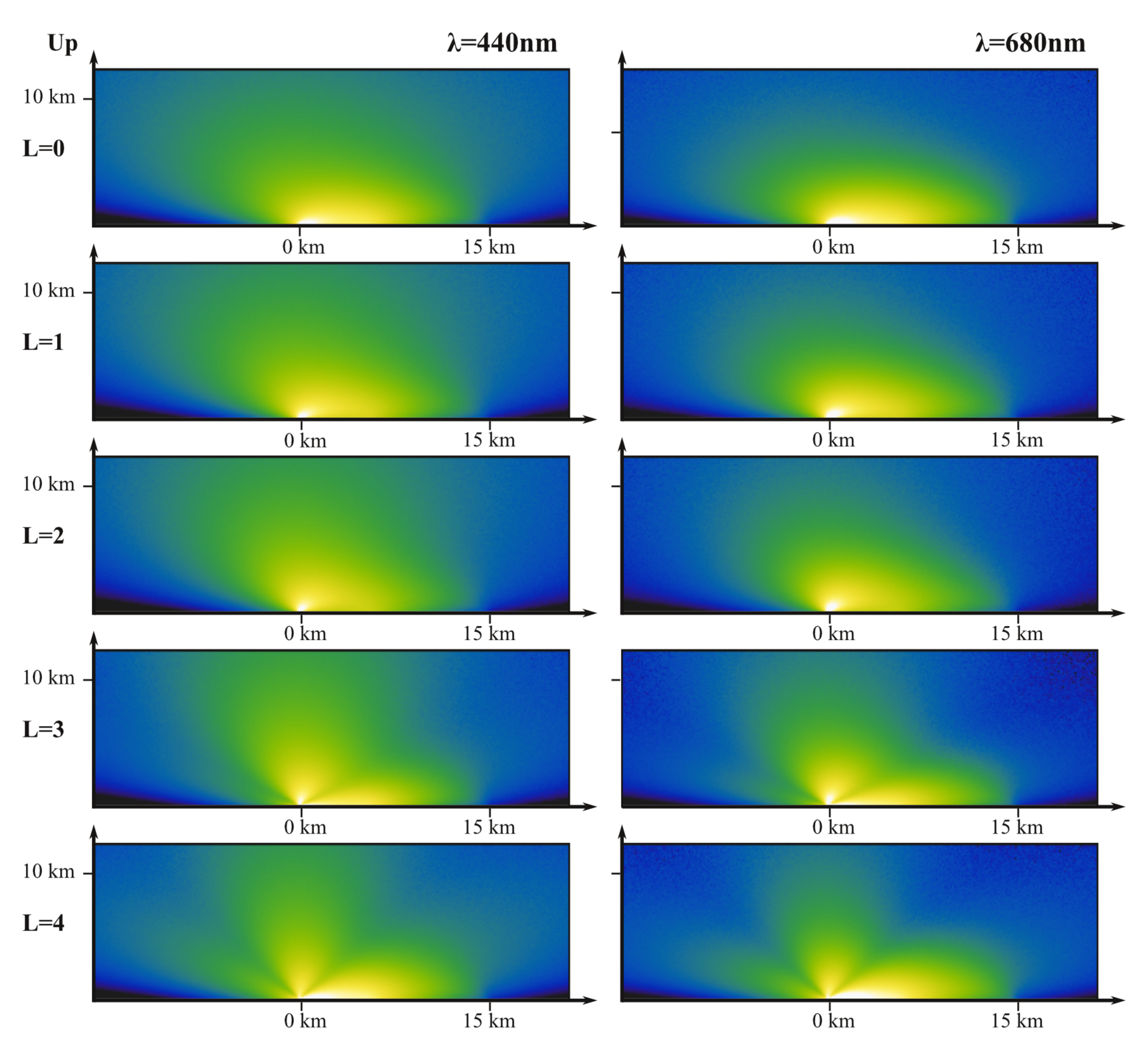
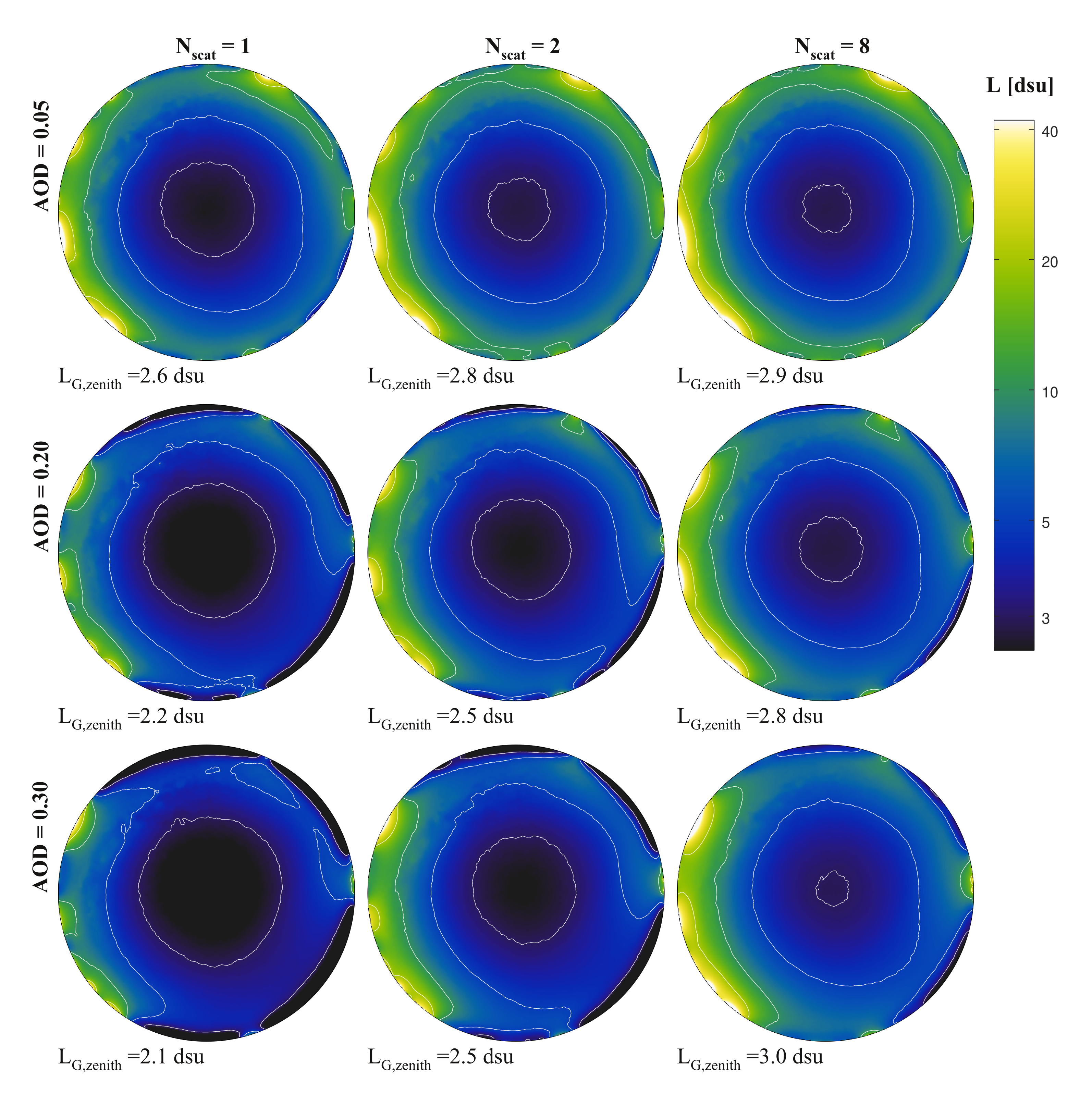
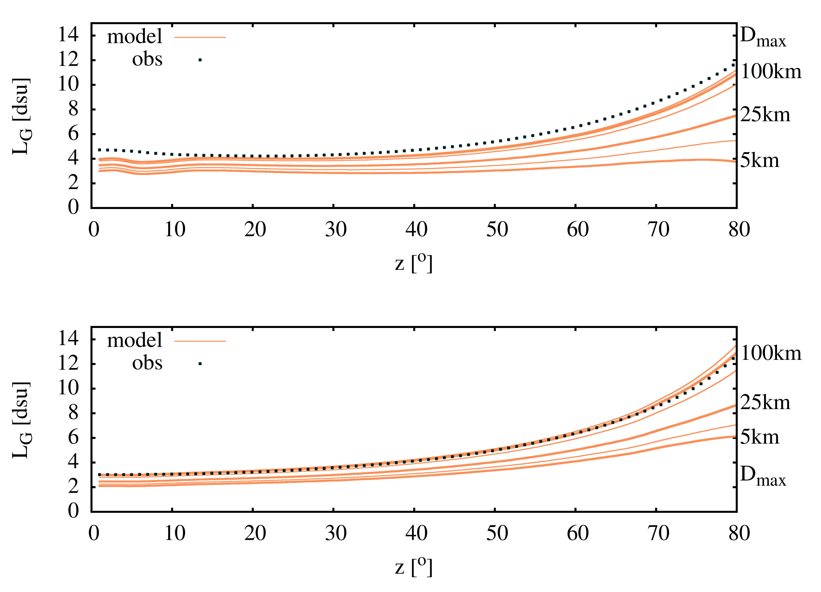
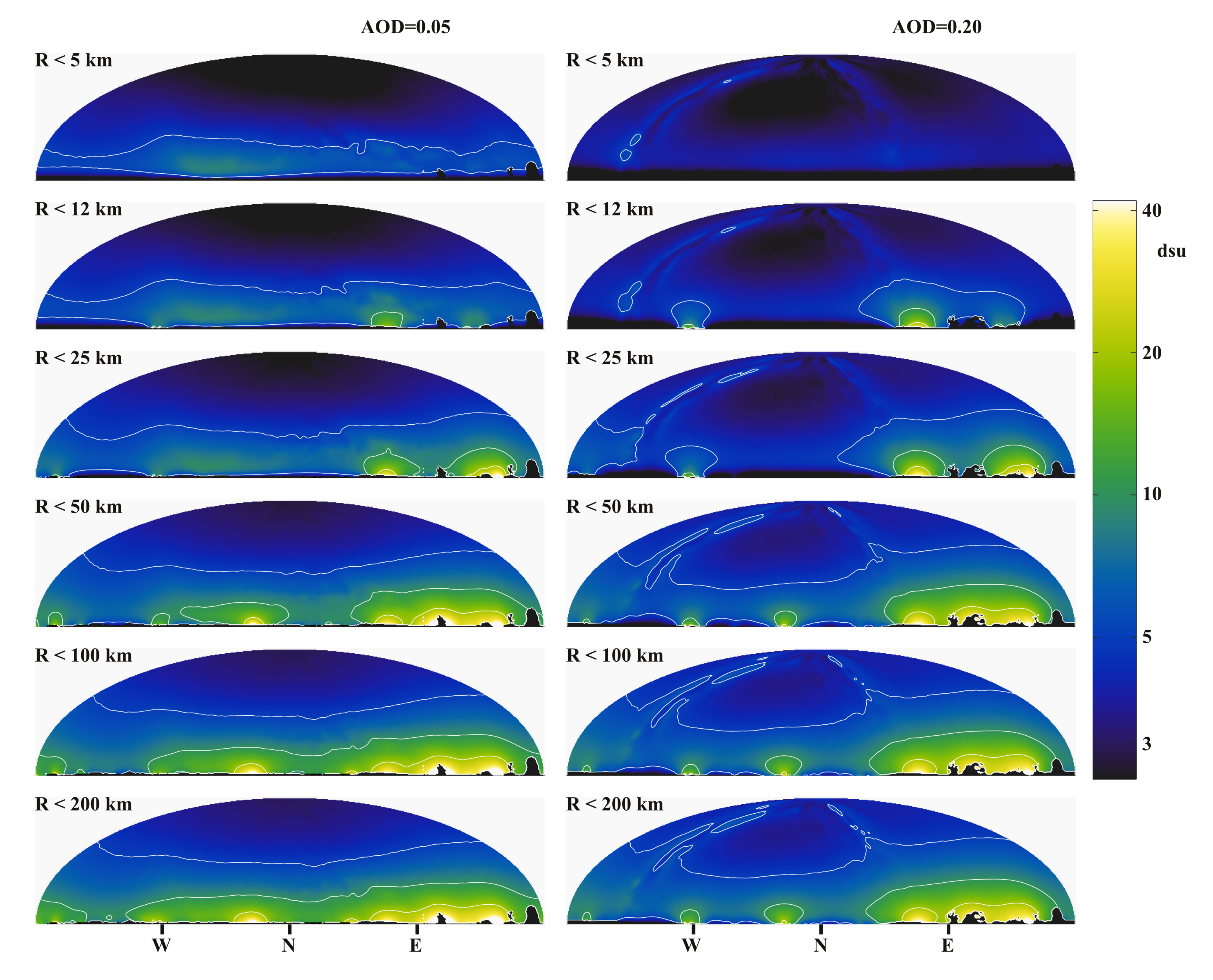
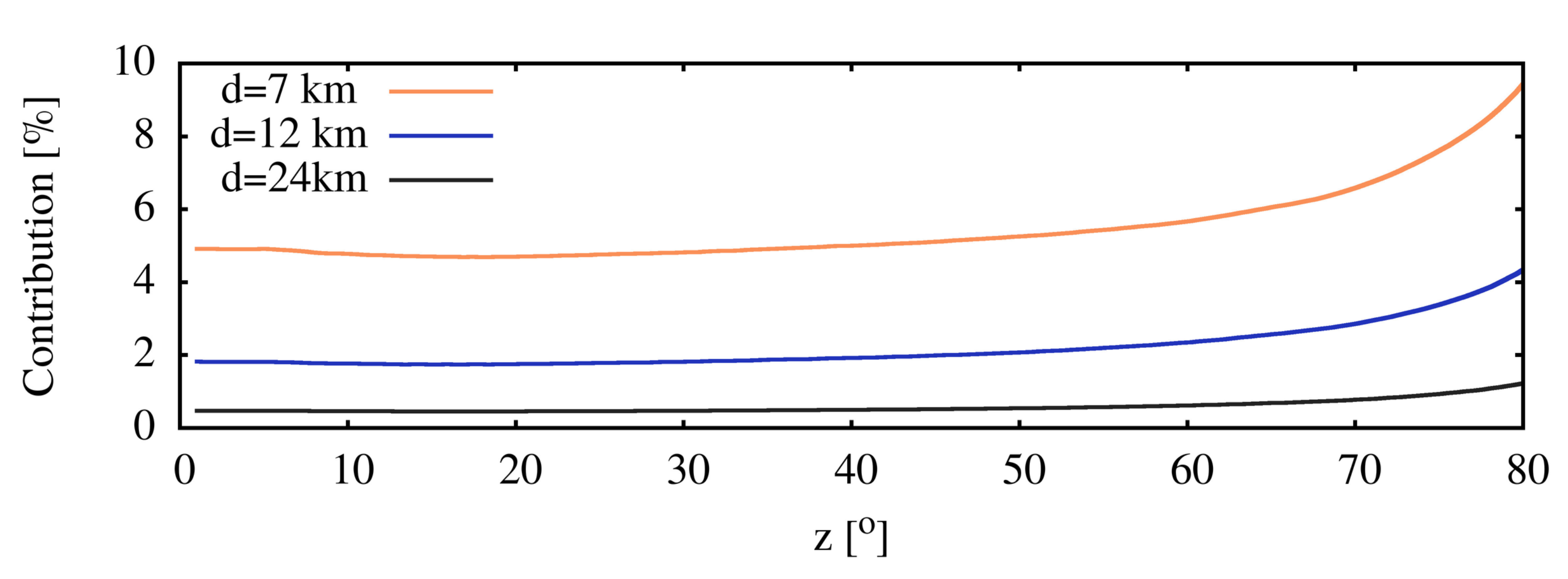
3.2. Dependence of Sky Radiance on the Distance of the Sources

When the overall fit of the models to the observations is satisfactory, we can use the Monte Carlo models to simulate the effect of only the subsets of all the sources. It is essential to know the contribution of sources at different distances from the observer to the sky brightness. The most straightforward application is to consider only sources within a given radius R. By increasing R, we can check how the effect of each settlement manifests itself. For the chosen observation site, a good possibility is that Budapest is within the distance range of 160–180 km, and the light path is not significantly shielded by topography.
Figure 11 displays how the radiance map of the sky depends on the maximum allowed distance of the sources for both optical depths used for the modelling.
There are no significant sources within 5 km, so the first row only illustrates the natural component of the sky based on the GAMBONS model. Within 10 km, two sources appear: the settlement of Hortobágy, which despite its proximity, does not represent significant light pollution. A larger city, Balmazújváros, provides a more substantial contribution to sky brightness. The satellite map displays another substantial source which is not a village but an industrial facility (Nagyhegyes Natural Gas Storage Site). Although having a much smaller geometrical extent than a settlement, it is a bright spot from space and provides a direct bright spot at the horizon. However, it does not contribute to the sky radiance as expected.
It is possible to create a weighted representation of the satellite light emission maps based on the fitted models. The weights are calculated according to the sky brightness excess produced by the given pixel and measured at a given geographic location. Figure 12 shows an example of this procedure. The modified map is shown weighted for two different observer locations. This further helps to identify the light domes in the ground measurements correctly. For the analyses in this article, we have used the 2019 VIIRS data, but for comparison purposes, here we also show the 2018 data. No significant differences between the two years are found, as confirmed by our additional tests.

4. Discussion

A major measure of light pollution at a given geographical location is the objective determination of night sky quality/radiance. Since multiple measurements are necessary to establish a firm foundation of the qualification, massive observational datasets exist at each location. However, the measurements are heterogeneous due to the varying atmospheric conditions. We developed a mapping technique based on ground-based and satellite observations combined with radiation transfer modelling to minimize sky quality determination uncertainties. Knowing the positions of light sources from satellite images, we could estimate the dark sky’s radiance with Monte Carlo radiation transfer modelling at specific sites. Then, we compared these simulations with actual measurements performed by DSLR cameras. The light output of the cities can be corrected by the measured spectra of the light domes to eliminate the mismatch due to the spectral response of satellite measurements. Then, an additional correction is made for the light output by fitting the observations. The natural night brightness is corrected by fitting to the data of the GAMBONS model. After determining the model parameters for a known location, we can easily extrapolate the parameters for another sites with similar environmental properties. With the combination of measurements and modelling, with a few physical measurements taken at different times and locations, we can create a high-quality light pollution map of a given protected area or other territories by extrapolation.
Our primary goal in fitting the observations was not to use the fitted parameters to determine the physical state of the atmosphere but to use the measurements to define a physically well-defined extrapolation procedure that can be used, for example, to map the area. If we can take measurements at one or a few locations and fit them to the models, we can use them to determine the sky’s state at any location. After fitting the global parameters, the models can be used to predict the effect of changes in environmental parameters. As an example, we show in Figure 13 the trends we expect to see as the AOD changes at the measurement site. We fitted the measurement with AOD = 0.05 and then calculated the distribution of sky radiances at that time in a less transparent atmosphere. We added a different location here, which has a more significant distance from the primary sources. It is close to Száztelek with coordinates: 47.5507 N–21.0639 E. As the AOD is increased, as expected, the light dome of distant settlements disappears steadily. Meanwhile, the models suggest that the measured radiances in the zenith do not change significantly. While the effect of remote sources decreases, nearby sources increase due to locally increased scattering.
We also provide a figure (Figure 14) with the profile of the mean radiance. The models are presented for all the components (orange curves) and the GAMBONS models only (blue curves). Note that the best fit of the observed zenith distance dependence does not coincide with the best topology in the sky radiance map. A possible resolution for this discrepancy is the effect of aerosol scale height.
Another application of models fitted to observations is the impact assessment of lighting in specific installations. There is a strong source visible over a significant part of the study area based on visual observations. This is the industrial area near Nagyhegyes mentioned above (coordinates: 47.5079 N–21.3666 E). Figure 15 illustrates how prominent this facility is compared to the light from other settlements from the observation point 24 km from the source. It also shows that the sky above it is not significantly brightened. Suppose the gas storage area is excluded from the sources considered in the model calculations. In that case, it is possible to estimate the facility’s contribution to the increase in sky brightness. In general, no significant variation can be observed in the sky radiance maps, but the increase is still observable. The percentage increase of sky radiance compared to the natural sky is shown in Figure 16. In addition to the two observation points used so far, we have also calculated the models for a closer location, 7 km away from the source (coordinates: 47.5095 N–21.2690 E). The figure demonstrates that a single facility can clearly degrade sky quality at an otherwise remote location. Compared to the actual (observed) sky radiance, the relative contribution reduced to half of the values presented in the figure.
We started to carry out additional measurements to determine the spectrum of sources in each municipality. We have developed a measurement system to determine the spectral composition of the light emitted by the lighting system with sufficient accuracy. This measurement device can be simply operated by driving a vehicle along the streets of a settlement. These data will allow us to fit satellite data to the spectrum. After fitting the spectral correction, we plan to use the comparison of measurements and models to fit individual corrections for each settlement. This procedure will also eliminate errors due to differences in spatial emission distributions. This work is under progress and will be published elsewhere.

5. Conclusions

We developed a Monte Carlo radiation transfer code that emphasises light pollution modelling. The new element of the procedure is the inclusion of an intermediate scattering density distribution. This method reduces the noise related to the scattering events close to the observers’ locations and makes it possible to interpolate the results smoothly to intermediate positions. The code is general enough to adapt it to different atmospheric conditions. Although the calculation of the scattering density distribution is CPU consuming, the resulting point spread function can be used to process night sky radiance maps for any source distribution quickly.
We also provide a procedure that results in the best model night sky distribution based on the available observational data. We use both spectral information and imaging radiometry of the upper hemisphere.
The best-fitted models can be calculated for a given location based on the spectral measurements and the corrected satellite observations. The model can be fine-tuned with the help of digital camera measurements. Thus the fits of all available data for a single location provide the best models to use to interpolate and extrapolate the ground-based measurements.
We have shown that sky radiances can be interpreted appropriately by combining all available information and using modern radiative transfer models. The maximum available information consists of the following components:
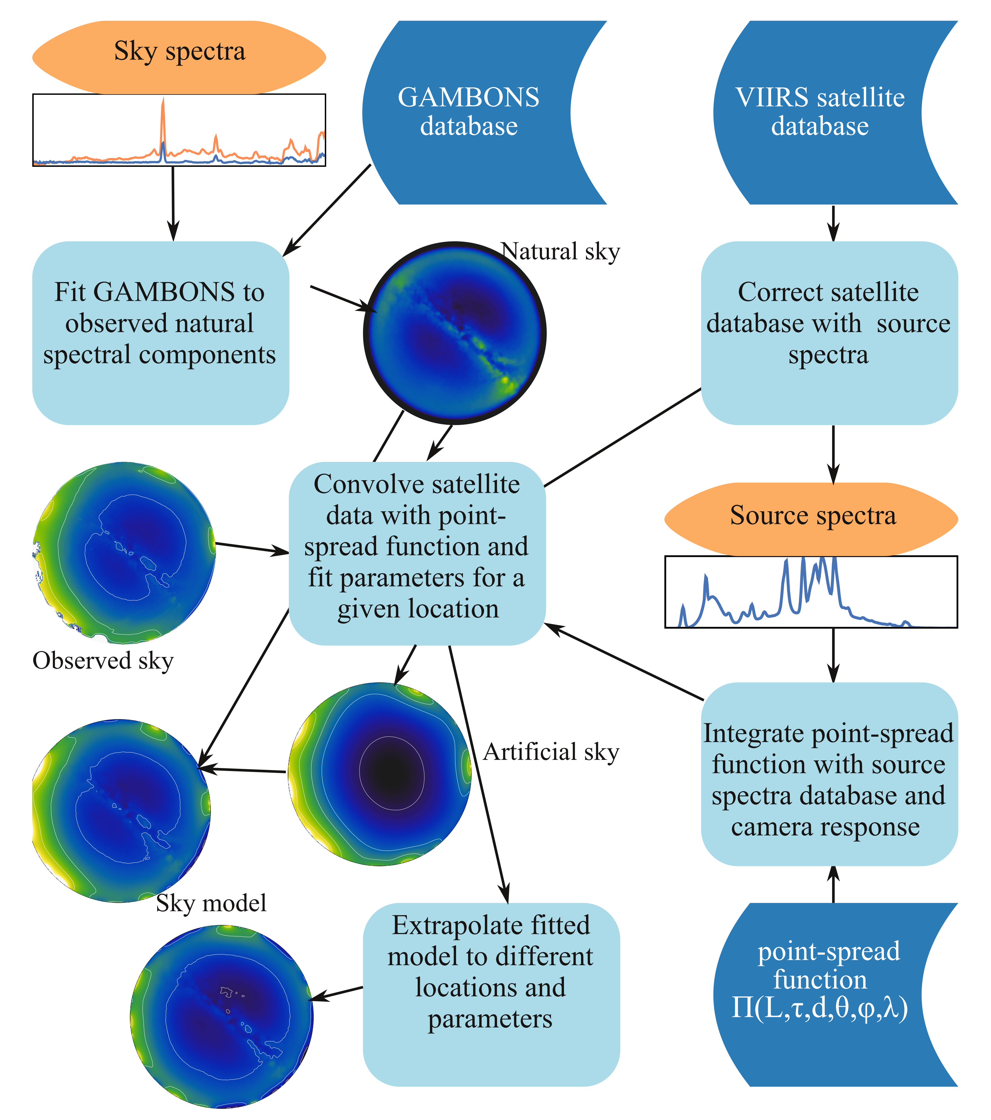
  • The natural distribution of the sky radiances, (GAMBONS)
  • The satellite measurements of the artificial light emission (VIIRS),
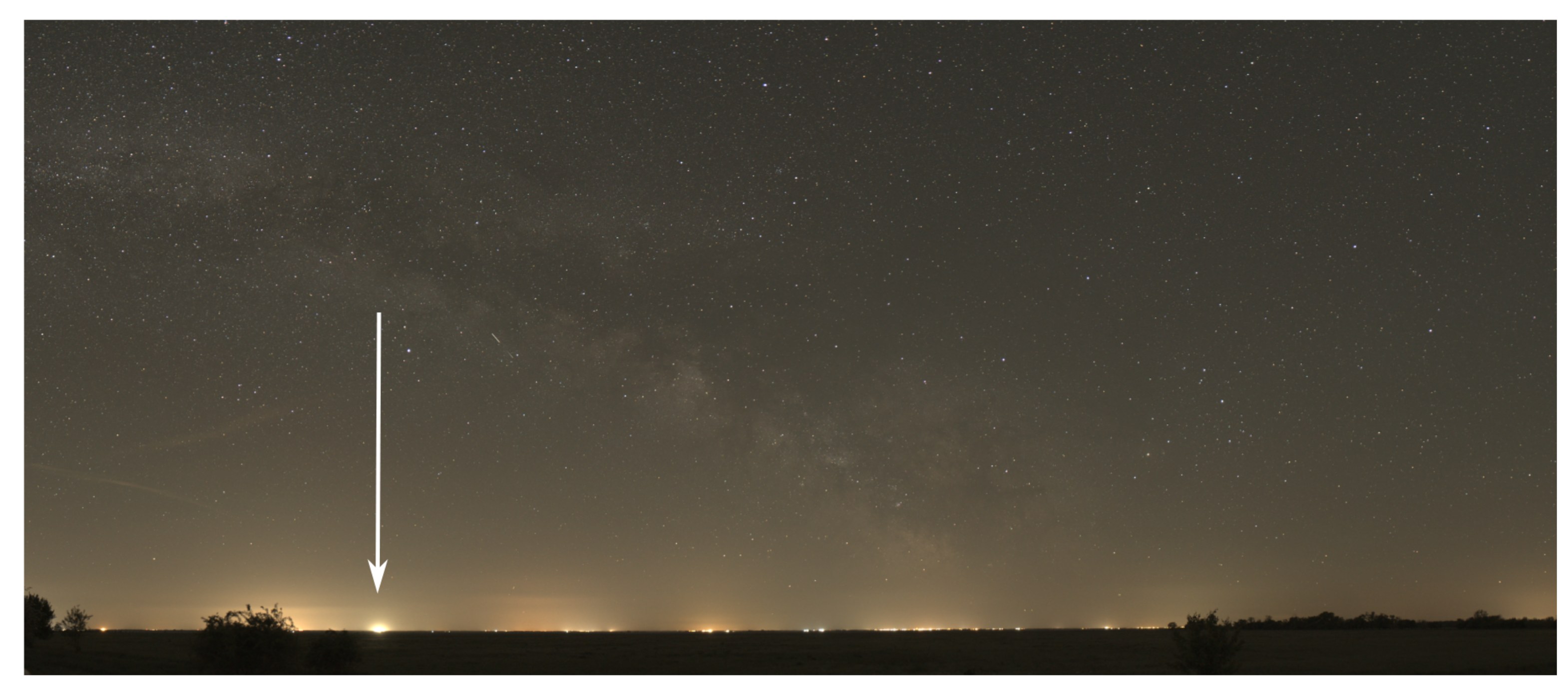
  • The distribution of the measured sky radiances, (DiCaLUM)
  • The distribution of the spectral radiances density of the sky at each location,
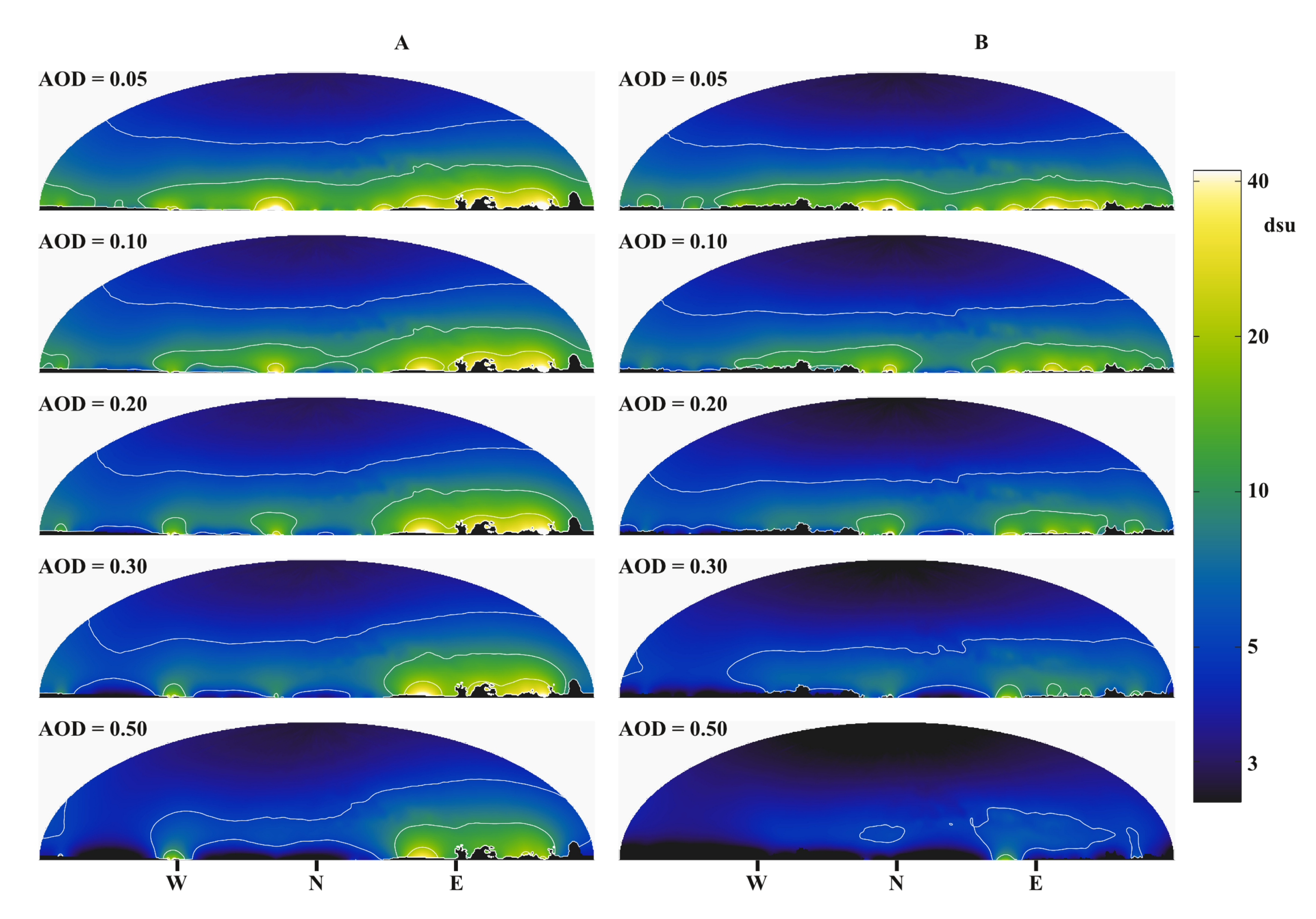
  • Sky radiances distribution based on radiative transfer models (ScatDenMC).
The combination of all this information has confirmed that the ScatDenMC model correctly describes the physical processes. The spectral information is essential for the interpretation of all-sky measurements and sky radiance modelling. The GAMBONS model was also crucial to make the comparison of observations and models firmly based.

Author Contributions

Conceptualization, Z.K., D.S. and K.K.; methodology, Z.K.; software, Z.K.; validation, D.S. and K.K.; measurements, D.S. and Z.K.; writing—original draft preparation, Z.K.; writing—review and editing, D.S. and K.K.; visualization, Z.K.; supervision, Z.K. All authors have read and agreed to the published version of the manuscript.

Funding

This research was funded by the European Union and co-financed by the European Social Fund (Grant No. EFOP–3.6.2–16–201–00014: Development of international research environment for light pollution studies) and the GINOP–2.3.3–15–2016–00037 project: Development of a measurement system based on digital cameras for international monitoring of light pollution and its biological effects.

Acknowledgments

We thank the Hortobágy National Park Directorate and István Gyarmathy for the help with the on-site measurements.

Conflicts of Interest

The authors declare no conflict of interest.

Abbreviations

The following abbreviations are used in this manuscript:
dsudark sky unit
FCEfalse colour enhancement
GAMBONSGAia Map of the Brightness Of the Natural Sky
DiCaLumDigital Camera Luminance
ScatDenMCScattering Density Monte Carlo (radiation transfer code)

References

  1. Cinzano, P. Night sky photometry with sky quality meter. ISTIL Int. Rep. 2005, 9, 1–14. [Google Scholar]
  2. Kolláth, Z.; Cool, A.; Jechow, A.; Kolláth, K.; Száz, D.; Tong, K.P. Introducing the Dark Sky Unit for multi-spectral measurement of the night sky quality with commercial digital cameras. J. Quant. Spectrosc. Radiat. Transf. 2020, 253, 107162. [Google Scholar] [CrossRef]
  3. Hänel, A.; Posch, T.; Ribas, S.J.; Aubé, M.; Duriscoe, D.; Jechow, A.; Kollath, Z.; Lolkema, D.E.; Moore, C.; Schmidt, N.; et al. Measuring night sky brightness: Methods and challenges. J. Quant. Spectrosc. Radiat. Transf. 2018, 205, 278–290. [Google Scholar] [CrossRef] [Green Version]
  4. Kolláth, Z. Measuring and modelling light pollution at the Zselic Starry Sky Park. J. Phys. Conf. Ser. 2010, 218, 012001. [Google Scholar] [CrossRef] [Green Version]
  5. Kolláth, Z.; Dömény, A.; Kolláth, K.; Nagy, B. Qualifying lighting remodelling in a Hungarian city based on light pollution effects. J. Quant. Spectrosc. Radiat. Transf. 2016, 181, 46–51. [Google Scholar] [CrossRef]
  6. Kolláth, Z.; Dömény, A. Night sky quality monitoring in existing and planned dark sky parks by digital cameras. Int. J. Sustain. Light. 2017, 19, 61–68. [Google Scholar] [CrossRef]
  7. Jechow, A.; Hölker, F.; Kolláth, Z.; Gessner, M.O.; Kyba, C.C.M. Evaluating the summer night sky brightness at a research field site on Lake Stechlin in northeastern Germany. J. Quant. Spectrosc. Radiat. Transf. 2016, 181, 24–32. [Google Scholar] [CrossRef] [Green Version]
  8. Jechow, A.; Ribas, S.J.; Domingo, R.C.; Hölker, F.; Kolláth, Z.; Kyba, C.C.M. Tracking the dynamics of skyglow with differential photometry using a digital camera with fisheye lens. J. Quant. Spectrosc. Radiat. Transf. 2018, 209, 212–223. [Google Scholar] [CrossRef] [Green Version]
  9. Jechow, A.; Hölker, F.; Kyba, C.C.M. Using all-sky differential photometry to investigate how nocturnal clouds darken the night sky in rural areas. Sci. Rep. 2019, 9, 1391. [Google Scholar] [CrossRef] [PubMed] [Green Version]
  10. Jechow, A.; Kyba, C.C.M.; Hölker, F. Mapping the brightness and color of urban to rural skyglow with all-sky photometry. J. Quant. Spectrosc. Radiat. Transf. 2020, 250, 106988. [Google Scholar] [CrossRef]
  11. Jechow, A.; Kyba, C.C.M.; Hölker, F. Beyond All-Sky: Assessing Ecological Light Pollution Using Multi-Spectral Full-Sphere Fisheye Lens Imaging. J. Imaging 2019, 5, 46. [Google Scholar] [CrossRef] [Green Version]
  12. Galatanu, C.D.; Husch, M.; Canale, L.; Lucache, D. Targeting the Light Pollution: A Study Case. In Proceedings of the 2019 IEEE International Conference on Environment and Electrical Engineering and 2019 IEEE Industrial and Commercial Power Systems Europe (EEEIC/I CPS Europe), Genova, Italy, 11–14 June 2019; pp. 1–6. [Google Scholar] [CrossRef]
  13. Kyba, C.C.M.; Hänel, A.; Hölker, F. Redefining efficiency for outdoor lighting. Energy Environ. Sci. 2014, 7, 1806. [Google Scholar] [CrossRef]
  14. Kyba, C.C.M.; Kuester, T.; Kuester, T. Changes in outdoor lighting in Germany from 2012–2016. Int. J. Sustain. Light. 2017, 19, 112–123. [Google Scholar] [CrossRef]
  15. Kyba, C.C.M.; Kuester, T.; De Miguel, A.S.; Baugh, K.; Jechow, A.; Hölker, F.; Bennie, J.; Elvidge, C.D.; Gaston, K.J.; Guanter, L. Artificially lit surface of Earth at night increasing in radiance and extent. Sci. Adv. 2017, 3, e1701528. [Google Scholar] [CrossRef] [PubMed] [Green Version]
  16. Davies, T.W.; Duffy, J.P.; Bennie, J.; Gaston, K.J. The nature, extent, and ecological implications of marine light pollution. Front. Ecol. Environ. 2014, 12, 347–355. [Google Scholar] [CrossRef] [Green Version]
  17. Davies, T.W.; Bennie, J.; Cruse, D.; Blumgart, D.; Inger, R.; Gaston, K.J. Multiple night-time light-emitting diode lighting strategies impact grassland invertebrate assemblages. Glob. Chang. Biol. 2017, 23, 2641–2648. [Google Scholar] [CrossRef] [PubMed]
  18. Davies, T.W.; Smyth, T. Why artificial light at night should be a focus for global change research in the 21st century. Glob. Chang. Biol. 2018, 24, 872–882. [Google Scholar] [CrossRef] [Green Version]
  19. Elvidge, C.D.; Zhizhin, M.; Ghosh, T.; Hsu, F.C.; Taneja, J. Annual Time Series of Global VIIRS Nighttime Lights Derived from Monthly Averages: 2012 to 2019. Remote Sens. 2021, 13, 922. [Google Scholar] [CrossRef]
  20. Elvidge, C.D.; Baugh, K.; Zhizhin, M.; Hsu, F.C.; Ghosh, T. VIIRS night-time lights. Int. J. Remote Sens. 2017, 38, 5860–5879. [Google Scholar] [CrossRef]
  21. Román, M.O.; Stokes, E.C. Holidays in lights: Tracking cultural patterns in demand for energy services. Earths Future 2015, 3, 182–205. [Google Scholar] [CrossRef]
  22. Sánchez de Miguel, A.; Kyba, C.C.; Aubé, M.; Zamorano, J.; Cardiel, N.; Tapia, C.; Bennie, J.; Gaston, K.J. Colour remote sensing of the impact of artificial light at night (I): The potential of the International Space Station and other DSLR-based platforms. Remote Sens. Environ. 2019, 224, 92–103. [Google Scholar] [CrossRef]
  23. Bouroussis, C.A.; Topalis, F.V. Assessment of outdoor lighting installations and their impact on light pollution using unmanned aircraft systems-The concept of the drone-gonio-photometer. J. Quant. Spectrosc. Radiat. Transf. 2020, 253, 107155. [Google Scholar] [CrossRef]
  24. Masana, E.; Carrasco, J.M.; Bará, S.; Ribas, S.J. A multiband map of the natural night sky brightness including Gaia and Hipparcos integrated starlight. Mon. Not. R. Astron. Soc. 2020, 501, 5443–5456. [Google Scholar] [CrossRef]
  25. Moncet, J.L.; Uymin, G.; Lipton, A.E.; Snell, H.E. Infrared Radiance Modeling by Optimal Spectral Sampling. J. Atmos. Sci. 2008, 65, 3917–3934. [Google Scholar] [CrossRef]
  26. Wang, C.; Yang, P.; Liu, X. A High-Spectral-Resolution Radiative Transfer Model for Simulating Multilayered Clouds and Aerosols in the Infrared Spectral Region. J. Atmos. Sci. 2015, 72, 926–942. [Google Scholar] [CrossRef]
  27. Liu, C.; Yao, B.; Natraj, V.; Weng, F.; Le, T.; Shia, R.L.; Yung, Y.L. A Spectral Data Compression (SDCOMP) Radiative Transfer Model for High-Spectral-Resolution Radiation Simulations. J. Atmos. Sci. 2020, 77, 2055–2066. [Google Scholar] [CrossRef] [Green Version]
  28. Kyba, C.C.M.; Aubé, M.; Bará, S.; Bertolo, A.; Bouroussis, C.A.; Cavazzani, S.; Espey, B.R.; Falchi, F.; Gyuk, G.; Jechow, A.; et al. The benefit of multiple angle observations for visible band remote sensing using night lights. Earth Sp. Sci . Open Arch. ESSOAr 2021. [Google Scholar] [CrossRef]
  29. Aubé, M.; Simoneau, A. New features to the night sky radiance model illumina: Hyperspectral support, improved obstacles and cloud reflection. J. Quant. Spectrosc. Radiat. Transf. 2018, 211, 25–34. [Google Scholar] [CrossRef]
  30. Kocifaj, M. Multiple scattering contribution to the diffuse light of a night sky: A model which embraces all orders of scattering. J. Quant. Spectrosc. Radiat. Transf. 2018, 206, 260–272. [Google Scholar] [CrossRef]
  31. Noebauer, U.M.; Sim, S.A. Monte Carlo radiative transfer. Living Rev. Comput. Astrophys. 2019, 5, 1. [Google Scholar] [CrossRef] [Green Version]
  32. Noll, S.; Kausch, W.; Barden, M.; Jones, A.M.; Szyszka, C.; Kimeswenger, S.; Vinther, J. An atmospheric radiation model for Cerro Paranal: I. The optical spectral range. Astron. Astrophys. 2012, 543, A92. [Google Scholar] [CrossRef]
  33. Spada, F.; Krol, M.C.; Stammes, P. McSCIA: Application of the Equivalence Theorem in a Monte Carlo radiative transfer model for spherical shell atmospheres. Atmos. Chem. Phys. 2006, 6, 4823–4842. [Google Scholar] [CrossRef] [Green Version]
Figure 1. Representations of digital camera measurements after DiCaLum processing. The top left image shows the original photographic montage of the upper hemisphere. FCE displays the same image with false colour enhancement, which amplifies the differences compared to a normal, natural sky. The Green channel radiance in the dsu unit is presented in the standard fish-eye projection and Hammer-Aitoff projection.
Remotesensing 13 03653 g001
Figure 2. Decomposition of the zenith sky spectrum to the natural and artificial components.
Remotesensing 13 03653 g002
Figure 3. Airglow radiance as a function of altitude. The lines show the GAMBONS model for high (orange) and low (blue) level of activity. The models are provided for two different solar activity levels (50% and 100% in the GAMBONS calculator) and for AOD = 0.05, 0.10, 0.20, 0.30 and 0.40 (from top to bottom). The labels next to the thick orange curves provide the corresponding AOD values. The black dots represent the actual measurements.
Remotesensing 13 03653 g003
Figure 4. Section of the scattering density distribution and its variation along a line (black curve). The radiance of the sky in a given direction (indicated by the white arrow) is given by the integral of the curve.
Remotesensing 13 03653 g004
Figure 5. Flowchart of the Monte Carlo simulation.
Remotesensing 13 03653 g005
Figure 6. Section of the scattering density distribution for different combinations of AOD and wavelength.(in the figure: the source is at 0 km, and the observer is at 15 km). The results depend on many parameters, like aerosol optical depth (AOD), density profile, etc.
Remotesensing 13 03653 g006
Figure 7. Dependence of calculated sky radiance on the number of scatterings.
Remotesensing 13 03653 g007
Figure 8. Flowchart of model fitting.
Remotesensing 13 03653 g008
Figure 9. The mean radiance of the sky as the function of the zenit distance. Top: first observation with AOD = 0.02; Bottom: second observation with AOD = 0.05. The models are calculated for the sources within a given distance. The limit distances are 5, 12, 25, 50, 100 and 200 km, from bottom to top. The limiting distance is indicated at the right side of the figure for the thick lines. The intermediate values for the thin lines are D m a x = 12 km and 50 km.
Remotesensing 13 03653 g009
Figure 10. Comparison of the observations (bottom) with the models (top) The areosol optical depth (AOD) used for the Monte Carlo simulation is indicated at the top of the figure.
Remotesensing 13 03653 g010
Figure 11. The build-up of the sky radiance vs the distance of included sources. The aerosol optical depth (AOD) used for the Monte Carlo simulation is indicated at the top of the figure. The maximum distance of the used sources is displayed at each row.
Remotesensing 13 03653 g011
Figure 12. Weighted source map based on the VIIRS images from 2018 and 2019 for two different observation points (indicated by arrows).
Remotesensing 13 03653 g012
Figure 13. The dependence of the sky radiance map on the atmospheric optical depths (AOD) for two different sites. (A): standard observing site; (B): location close to Szásztelek.
Remotesensing 13 03653 g013
Figure 14. The mean radiance of the sky as the function of the zenith distance and AOD. The blue lines represent only the natural component (GAMBONS model). The AOD is indicated at the right side of the figure for the thick lines. The intermediate values for the thin lines are AOD = 0.1 and 0.3.
Remotesensing 13 03653 g014
Figure 15. View on the horizon at the second observation point close to Szásztelek. The white arrow indicates the light of the gas storage station.
Remotesensing 13 03653 g015
Figure 16. The relative contribution of the gas storage facility to the sky radiance compared to the natural sky from three different distances.
Remotesensing 13 03653 g016
Publisher’s Note: MDPI stays neutral with regard to jurisdictional claims in published maps and institutional affiliations.

