
Guaranteed Robust Tensor Completion via ∗L-SVD with Applications to Remote Sensing Data


1
School of Automation, Guangdong University of Technology, Guangzhou 510006, China
2
Tensor Learning Team, RIKEN AIP, Tokyo 103-0027, Japan
3
Key Laboratory of Intelligent Detection and The Internet of Things in Manufacturing, Ministry of Education, Guangzhou 510006, China
*
Author to whom correspondence should be addressed.
Remote Sens. 2021, 13(18), 3671; https://0-doi-org.brum.beds.ac.uk/10.3390/rs13183671
Submission received: 30 July 2021
/
Revised: 3 September 2021
/
Accepted: 9 September 2021
/
Published: 14 September 2021
(This article belongs to the Special Issue Remote Sensing Image Denoising, Restoration and Reconstruction)
Abstract
:This paper conducts a rigorous analysis for the problem of robust tensor completion, which aims at recovering an unknown three-way tensor from incomplete observations corrupted by gross sparse outliers and small dense noises simultaneously due to various reasons such as sensor dead pixels, communication loss, electromagnetic interferences, cloud shadows, etc. To estimate the underlying tensor, a new penalized least squares estimator is first formulated by exploiting the low rankness of the signal tensor within the framework of tensor -Singular Value Decomposition (-SVD) and leveraging the sparse structure of the outlier tensor. Then, an algorithm based on the Alternating Direction Method of Multipliers (ADMM) is designed to compute the estimator in an efficient way. Statistically, the non-asymptotic upper bound on the estimation error is established and further proved to be optimal (up to a log factor) in a minimax sense. Simulation studies on synthetic data demonstrate that the proposed error bound can predict the scaling behavior of the estimation error with problem parameters (i.e., tubal rank of the underlying tensor, sparsity of the outliers, and the number of uncorrupted observations). Both the effectiveness and efficiency of the proposed algorithm are evaluated through experiments for robust completion on seven different types of remote sensing data.

1. Introduction
Despite the broad adoption of advanced sensors in various remote sensing tasks, the quality of data remains a critical issue and can significantly influence the actual performances of the backend applications. Many types of modern remote sensing data in the modality of optical, hyperspectral, multispectral, thermal, Light Detection and Ranging (LiDAR), Synthetic Aperture Radar (SAR), etc., are typically multi-way and can be readily stored, analyzed, and processed by tensor-based models [1,2,3,4,5,6,7]. In some extreme circumstances, the data tensor may encounter missing entries, gross sparse outliers, and small dense noises at the same time, as a result of partial sensor failures, communication errors, occlusion by obstacles, and so on [8,9]. To robustly complete a partially observed data tensor corrupted by outliers and noises, the problem of robust tensor completion arises.
When only a fraction of partially corrupted observations are available, the crucial point of robust tensor completion lies in the assumption that the underlying data tensor is highly redundant such that the main components of it remain only slightly suppressed by missing information, outliers, and noises, and thus can be effectively reconstructed by exploiting the intrinsic redundancy. The tensor low-rankness is an ideal tool to model the redundancy of tensor data, and has gained extensive attention in remote sensing data restoration [5,10,11].
As higher-order extensions of low-rank matrix models [12], low-rank tensor models are typically formulated as minimization problems of the tensor rank function [13]. However, there are multiple definitions of tensor ranks, such as the CP rank [14], Tucker rank [15], TT rank [16], TR rank [17], etc., which focus on low rank structures in the original domains (like the pixel domain of optimal images) [18,19]. Recently, a remarkably different example named the low-tubal-rank tensor model [20,21] was proposed within the algebraic framework of tensor Singular Value Decomposition (t-SVD) [20,22], which captures low-rankness in the frequency domain defined via Discrete Fourier Transform (DFT). As discussed in [18,19,21,23], the low-tubal-rank tensor models are capable to exploit both low-rankness and smoothness of the tensor data, making it quite suitable to analyze and process diverse remote sensing imagery data which are often simultaneously low-rank and smooth [5,10].
Motivated by the advantages of low-tubal-rankness in modeling remote sensing data, we resolve the robust tensor completion problem by utilizing a generalized low-tubal-rank model based on the tensor -Singular Value Decomposition (-SVD) [24], which leverages low-rankness in more general transformed domains rather than DFT. What needs to be pointed out is that the -SVD has become a research focus in tensor-based signal processing, computer vision, and machine learning very recently [18,23,25,26]. Regarding the preference of theory in this paper, we only introduce several typical works with statistical analysis as follows. For tensor completion in the noiseless settings, Lu et al. [26] proposed a -SVD-based model which can exactly recover the underlying tensor under mild conditions. For tensor completion from partial observations corrupted by sparse outliers, Song et al. [27] designed a -SVD-based algorithm with exact recovery guarantee. Zhang et al. [25] developed a theoretically guaranteed approach via the -SVD to for tensor completion from Poisson noises. The problem of tensor recovery from noisy linear observations is studied in [18] based the -SVD with guaranteed statistical performance.
In this paper, we focus on statistical guaranteed approaches in a more challenging setting than the aforementioned -SVD-based models, where the underlying signal tensor suffers from missing entries, sparse outliers, and small dense noises simultaneously. Specifically, we resolve the problem of robust tensor completion by formulating a -SVD-based estimator whose estimation error is established and further proved to be minimax optimal (up to a log factor). We propose an algorithm based on Alternating Direction Method of Multipliers (ADMM) [28,29] to compute the estimator and evaluate both the effectiveness and efficiency on seven different types of remote sensing data.
The remainder of this paper proceeds as follows. We first introduce some notation and preliminaries in Section 2. Then, the proposed estimator for robust tensor completion is formulated in Section 3. We compute the estimator by using an ADMM-based algorithm described in Section 4. The statistical performance of the proposed estimator is analyzed in Section 5. Experimental results on both synthetic and real datasets are reported in Section 7. We summarize this paper and discuss future directions briefly in Section 8. The proofs of the theoretical results are given in Appendix A.
2. Preliminaries
In this section, we first introduce some notations and then give a brief introduction to the -SVD framework.
2.1. Notations
Main notations are listed in Table 1. Let , . Let and , . For denotes the standard vector basis whose entry is 1 with the others 0. For , the outer product denotes a standard tensor basis in , whose entry is 1 with the others 0. For a 3-way tensor, a tube is a vector defined by fixing indices of the first two modes and varying the third one; A slice is a matrix defined by fixing all but two indices. For any set , denotes its cardinality and its complement. Absolute positive constants are denoted by , whose values may vary from line to line. When the field and size of a tensor are not shown explicitly, it is defaulted to be in . The spectral norm and nuclear norm of a matrix are the maximum and the sum of the singular values, respectively.
2.2. Tensor -Singular Value Decomposition
The tensor -SVD is a generalization of the t-SVD [22]. To get a better understanding of -SVD, we first introduce several basic notions of t-SVD as follows. For any tensor , its block circulant matrix is defined as
We also define the block vectorization operator and its inverse operator for any by:
Then, based on the operators defined above, we are able to give the definition of the tensor t-product.
Definition 1
If we view the 3-way tensor as a -by- “matrix” of tubes , then the t-product can be analogously conducted like the matrix multiplication by changing scalar multiplication by the circular convolution between the tubes (i.e., vectors), as follows:
where the symbol ⊛ denotes the circular convolution of two tubes defined as follows [22]:
where is the modulus operator. According to the well-known relationship between circular convolution and DFT, the t-product is equivalent to matrix multiplication between all the frontal slices in the Fourier domain [22], i.e.,
where denotes the tensor obtained by conducting DFT on all the mode-3 fibers of any tensor , i.e.,
where is the transform matrix of DFT [22], and denotes the tensor mode-3 product [30].
In [24], Kernfeld et al. extended the t-product to the tensor -product by replacing DFT by any invertible linear transform induced by a non-singular transformation matrix , and established the framework of -SVD. In the latest studies, the transformation matrix defining the transform L is restricted to be orthogonal [18,26,31,32] (unitary in [25,27]) for better properties, which is also followed in this paper.
Given any orthogonal matrix (though we restrict to be orthogonal for simplicy, our analysis still holds with simple extensions for unitary [27]), define the associated linear transform with inverse on any as
Definition 2
Definition 3
(–block-diagonal matrix [18]). For any , its –block-diagonal matrix, denoted by , is defined as the block diagonal matrix whose i-th diagonal block is the i-th frontal slice of , i.e.,
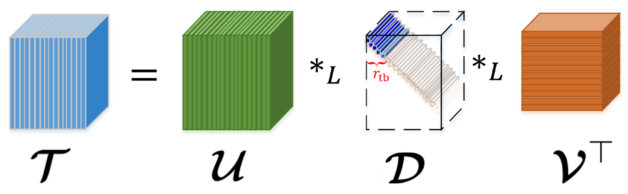
Based on the notions of tensor –transpose, -identity tensor, -orthogonal tensor, and f-diagonal tensor [24], the –SVD (illustrated in Figure 1) is given.
Theorem 1
(Tensor –SVD, -tubal rank [24]). Any has a tensor –Singular Value Decomposition (–SVD) under any L in Equation (4), given as follows
where , are -orthogonal, and is f-diagonal.
The -tubal rank of is defined as the number of non-zero tubes of in its –SVD in Equation (5) i.e.,
where # counts the number of elements of a given set.
For any , we have the following equivalence between its -SVD and the matrix SVD of its –block-diagonal matrix :
Considering the block diagonal structure of , we define the tensor -multi-rank on its diagonal blocks :
Definition 4
As proved in [26,27], –TNN is the convex envelop of the -norm of the –multi-rank in unit tensor -spectral norm ball. Thus, –TNN encourages a low –multi-rank structure which means low-rankness in spectral domain. When the linear transform L represents the DFT (although we restrict the in Equation (4) to be orthogonal, we still consider TNN as a special case of –TNN up to constants and real/complex domain) along the 3-rd mode, –TNN and tensor -spectral norm degenerate to the Tubal Nuclear Norm (TNN) and the tensor spectral norm, respectively, up to a constant factor [26,33].
3. Robust Tensor Completion
In this section, we will formulate the robust tensor completion problem. The observation model will be shown first.
3.1. The Observation Model
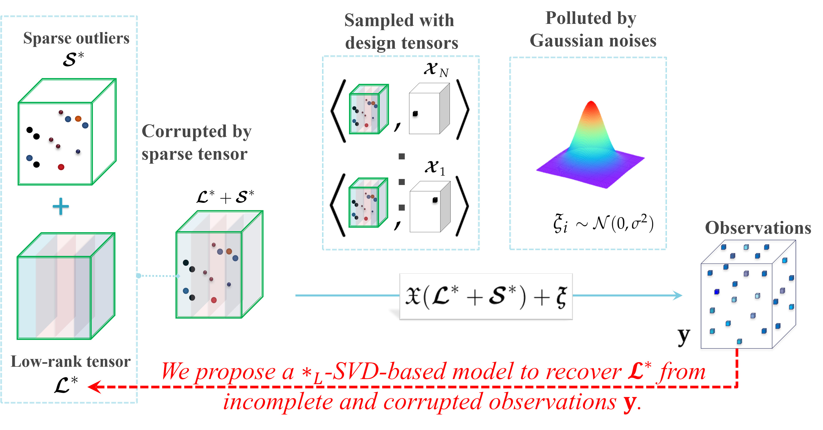
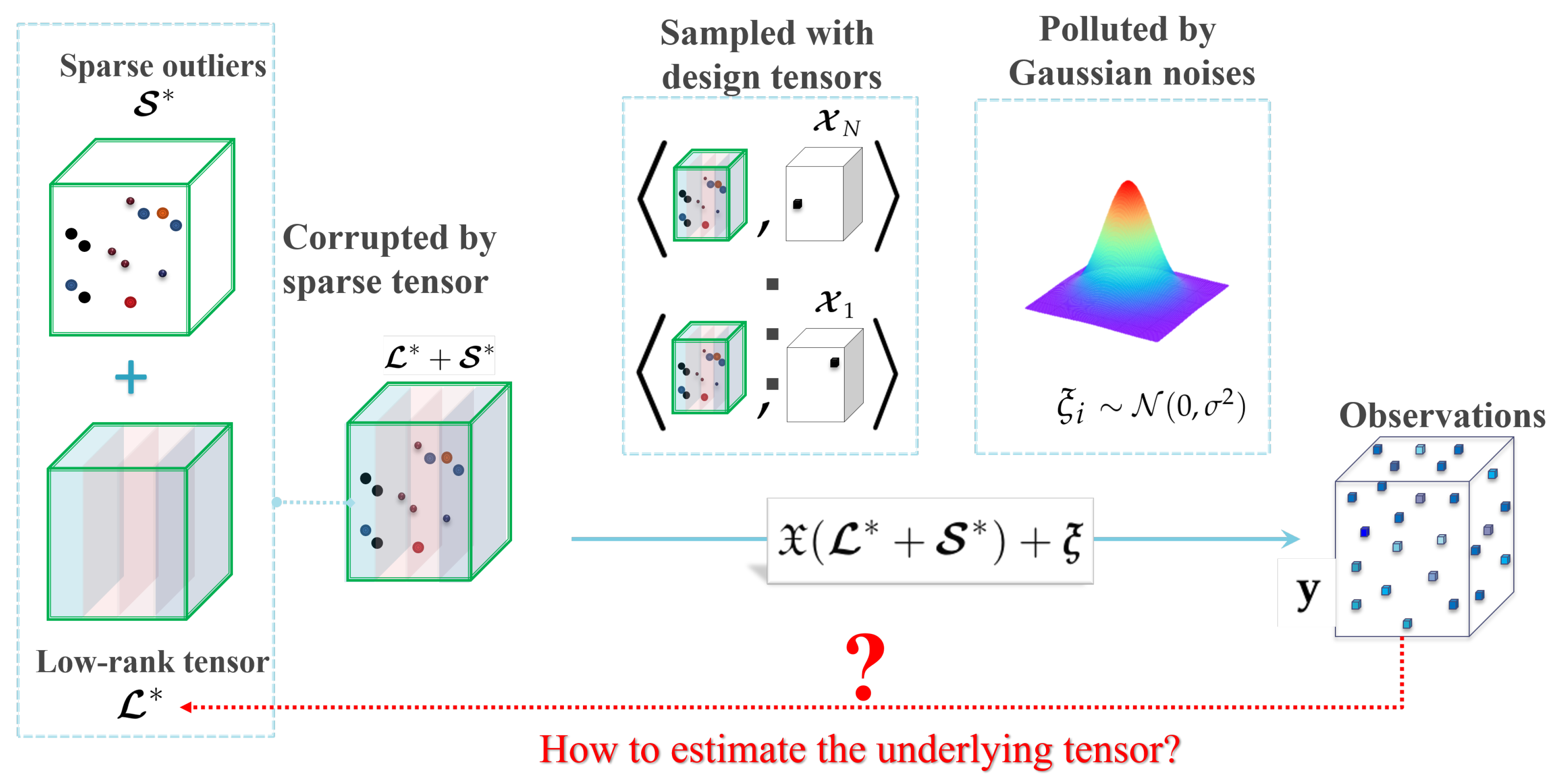
Consider an underling signal tensor which possesses intrinsically low-dimensionality structure characterized by low-tubal-rankness, that is . Suppose we obtain N scalar observations of from the noisy observation model:
where the tensor represents some gross corruptions (e.g., outliers, errors, etc.) additive to the signal which is element-wisely sparse (the presented theoretical analysis and optimization algorithm can be generalized to more sparsity settings of corruptions (e.g. the tube-wise sparsity [20,34], and slice-wise sparsity [34,35]) by using the tools developed for robust matrix completion in [36] and robust tensor decomposition in [34]; for simplicity, we only consider the most common element-wisely sparse case), ’s are random noises sampled i.i.d. from Gaussian distribution , and ’s are known random design tensors in satisfying the following assumptions:
Assumption A1.
We make two natural assumptions on the design tensors:
- I.
- All the corrupted positions of are observed, that is, the (unknown) support of the corruption tensor is fully observed. Formally speaking, there exists an unknown subset drawn from an (unknown) distribution on the set , such that each element in is sampled at least once.
- II.
- All uncorrupted positions of are sampled uniformly with replacement for simplicity of exposition. Formally speaking, each element of the set is sampled i.i.d. from an uniform distribution on the set .
According to the observation model (6), the true tensor is first corrupted by a sparse tensor and then sampled to N scalars with additive Gaussian noises (see Figure 2). The corrupted positions of are further assumed in Assumption A1 to be totally observed with design tensors in , and the remaining uncorrupted positions are sampled uniformly through design tensors in .
Let and be the vector of observations and noises, respectively. Define the design operator as and its adjoint operator for any . Then the observation model (6) can be rewritten in a compact form
3.2. The Proposed Estimator
The aim of robust tensor completion is to reconstruct the unknown low-rank and sparse from incomplete and noisy measurements generated by the observation model (6). It can be treated as a robust extension of tensor completion in [33], and a noisy partial variant of tensor robust PCA [37].
To reconstruct the underlying low-rank tensor and sparse tensor , it is natural to consider the following minimization model:
where we use least squares as the fidelity term for Gaussian noises, the tubal rank as the regularization to impose low-rank structure in , the tensor -(pseudo)norm to regularize for sparsity, are tunable regularization parameters, balancing the regularizations and the fidelity term.
However, general rank and -norm minimization is NP-hard [12,38], making it extremely hard to soundly solve Problem (7). For tractable low-rank and sparse optimization, we follow the most common idea to relax the non-convex functions and to their convex surrogates, i.e., the –tubal nuclear norm and the tensor -norm , respectively. Specifically, the following estimator is defined:
where is a known constant constraining the magnitude of entries in and . The additional constraint and is very mild since most signals and corruptions are of limited energy in real applications. It can also provide a theoretical benefit to exclude the “spiky” tensors, which is important in controlling the separability of and . Such “non-spiky” constraints are also imposed in previous literatures [36,39,40], playing a key role in bounding the estimation error.
Then, it is natural to ask the following questions:
- Q1:
- How to compute the proposed estimator?
- Q2:
- How well can the proposed estimator estimate and ?
4. Algorithm
In this section, we answer Q1 by designing an algorithm based on ADMM to compute the proposed estimator.
To solve Problem (8), the first step is to introduce auxiliary variables to deal with the complex couplings between , , , and as follows:
where is the indicator function of tensor -norm ball defined as follows
We then give the augmented Lagrangian of Equation (9) with Lagrangian multipliers and and penalty parameter :
Following the framework of standard two-block ADMM [41], we separate the primal variables into two blocks and , and update them alternatively as follows:
Update the first block : After the t-th iteration, we first update by keeping the other variables fixed as follows:
By taking derivatives, respectively, to and and setting them to zero, we obtain the following system of equations:
Through solving the system of equations in Equation (12), we obtain
where denotes the identity operator, and the intermediate tensors are given by , , and .
Update the second block : According to the special form of the Lagrangian in Equation (10), the variables in the second block can be updated separately as follows.
We first update with fixed :
We then update with fixed :
where is the proximality operator of –TNN given in the following lemma.
Lemma 1
(A modified version of Theorem 3.2 in [26]). Let be any tensor with –SVD . Then the proximality operator of –TNN at with constant , defined as , can be computed by
where
where denotes the positive part of t, i.e., .
We update with fixed :
where is the proximality operator [19] of the tensor -norm at point given as , where ⊙ denotes the element-wise product.
We then update with fixed :
where is the projector onto the tensor -norm ball of radius a, which is given by [19].
Similarly, we update as follows:
Update the dual variables and : According to the update strategy of dual variables in ADMM [41], the variables and can be updated using dual ascent as follows:
The algorithm for solving Problem (8) is summarized in Algorithm 1.
| Algorithm 1 Solving Problem (8) using ADMM. |
|
Complexity Analysis: The time complexity of Algorithm 1 is analyzed as follows. Due to the special structures of design tensors , the operators and can be implemented with time cost and , respectively. The cost of updating and is . The main time cost in Algorithm 1 lies in the update of which needs the –SVD on tensors, involving the -transform (costing in general), and matrix SVDs on matrices (costing ). Thus, the one-iteration cost of Algorithm 1 is
in general, and can be reduced to for some linear transforms L which have fast implementations (like DFT and DCT).
Convergence Analysis: According to [28], the convergence rate of general ADMM-based algorithms is , where t is the iteration number. The convergence analysis of Algorithm 1 is established in Theorem 2.
Theorem 2
Proof.
The key idea is to rewrite Problem (9) into a standard two-block ADMM problem. For notational simplicity, let
with and defined as follows
and
where denotes the operation of tensor vectorization (see [30]).
It can be verified that and are closed, proper convex functions. Then, Problem (9) can be re-written as follows:
According to the convergence analysis in [41], we have:
where are the optimal values of , , respectively. Variable is a dual optimal point defined as:
where is the component of dual variables in a saddle point
of the unaugmented Lagrangian
. □
5. Statistical Performance
In this section, we answer Q2 by studying the statistical performances of the proposed estimator . Specifically, the goal is to upper bound the squared F-norm error . We will first give an upper bound on the estimation error in a non-asymptotic manner, and then prove that the upper bound is minimax optimal up to a logarithm factor.
5.1. Upper Bound on the Estimation Error
We establish an upper bounds on the estimation error in the following theorem. For notational simplicity, let and denote the number of corrupted and uncorrupted observations of in the observation model (6), respectively.
Theorem 3
Theorem 3 implies that, if the noise level and spikiness level a are fixed, and all the corrupted positions are observed exactly only once (i.e., the number of corrupted observations ), then the estimation error in Equation (26) would be bounded by
Note that, the bound in Equation (27) is intuition-consistent: if the underlying tensor gets more complex (i.e., with higher tubal rank), then the estimation error will be larger; if the corruption tensor gets denser, then the estimation error will also become larger; if the number of uncorrupted observations gets larger, then the estimation error will decrease. The scaling behavior of the estimation error in Equation (27) will be verified through experiments on synthetic data in Section 7.1.
Remark 1
(Consistence with prior models for robust low-tubal-rank tensor completion). According to Equation (27), our –SVD-based estimator in Equation (8) allows the tubal rank to take the order , and the corruption ratio to be for approximate estimation with small error. It is slightly better with a logarithm factor than the results for t-SVD-based tensor robust completion model in [8] which allows and .
Remark 2
Remark 3
(Consistence with prior models for robust low-tubal-rank tensor decomposition). In the setting of Robust Tensor Decomposition (RTD) [34], the fully observed model instead of our estimation model in Equation (6) is considered. For the RTD problem, our error bound in Equation (27) is consistent with the t-SVD-based bound for RTD [34] (up to a logarithm factor).
Remark 4
(No exact recovery guarantee). According to Theorem 3, when and , i.e., in the noiseless case, the estimation error is upper bounded by which is not zero. Thus, no exact recovery is guaranteed by Theorem 3. It can be seen as a trade-off that we do not assume the low-tubal-rank tensor to satisfy the tensor incoherent conditions [8,35,37] which essentially ensures the separability between and .
5.2. A Minimax Lower Bound for the Estimation Error
In Theorem 3, we established the estimation error for Model (8). Then one may ask the complementary questions: how tight is the upper bound? Are there fundamental (model-independent) limits of estimation error in robust tensor completion? In this section, we will answer the questions.
To analyze the optimality of the proposed upper bound in Theorem 3, the minimax lower bounds of the estimation error is established for the tensor pair belonging to the class of tensor pairs defined as:
We then define the associated element-wise minimax error as follows
where the infimum ranges over all pairs of estimators , the supremum ranges over all pairs of underlying tensors in the given tensor class , and the expectation is taken over the design tensors and i.i.d. Gaussian noises in the observation model (6). We come up with the following theorem.
Theorem 4
(Minimax lower bound). Suppose the dimensionality , the rank and sparsity parameters , the number of uncorrupted entries , and the number of corrupted entries with a constant . Then, under Assumption A1, there exist absolute constants and , such that
where
The lower bound given in Equation (30) implies that the proposed upper bound in Theorem 3 is optimal (up to a log factor) in the minimax sense for tensors belonging to the set . That is to say no estimator can obtain more accurate estimation than our estimator in Equation (8) (up to a log factor) for , thereby showing the optimality of the proposed estimator.
6. Connections and Differences with Previous Works
In this section, we discuss the connections and differences with existing nuclear norm based robust matrix/tensor completion models, where the underlying matrix/tensor suffers from missing values, gross sparse outliers, and small dense noises at the same time.
First, we briefly introduce and analyze the two most related models, i.e., the matrix nuclear norm based model [36] and the sum of mode-wise matrix nuclear norms based model [45] as follows.
- (1)
- The matrix Nuclear Norm (NN) based model [36]: If the underlying tensor is of 2-way, i.e., a matrix, then the observation model in Equation (6) becomes the setting for robust matrix completion, and the proposed estimator in Equation (8) degenerates to the matrix nuclear norm based estimator in [36]. In both model formulation and statistical analysis, this work can be seen as a 3-way generalization of [36].Moreover, by conducting robust matrix completion on each frontal slice of a 3-way tensor, we can obtain the matrix nuclear norm based robust tensor completion model as follows:
- (2)
- The Sum of mode-wise matrix Nuclear Norms (SNN) based model [45]: Huang et al. [45] proposed a robust tensor completion model based on the sum of mode-wise nuclear norms deduced by the Tucker decomposition as followswhere is the mode-k matriculation of tensor , for all .The main differences between SNN and this work are two-fold: (i) SNN is based on the Tucker decomposition [15], whereas this work is based on the recently proposed tensor -SVD [24]; (ii) the theoretical analysis for SNN cannot guarantee the minimax optimality of the model in [45], whereas this works rigorously proof of the minimax optimality of the proposed estimator is established in Section 5.
Then, we discuss the following related works which can be seen as special cases of this work.
- (1)
- The robust tensor completion model based on t-SVD [46]: In a short conference presentation [46] (whose first author is the same as this paper), the t-SVD-based robust tensor completion model is studied. As t-SVD can be viewed as a special case of the -SVD (when DFT is used as the transform L), the model in [46] can be a special case of ours.
- (2)
- The robust tensor recovery models with missing values and sparse outliers [8,27]: In [8,27], the authors considered the robust reconstruction of incomplete tensor polluted by sparse outliers, and proposed t-SVD (or -SVD) based models with theoretical guarantees for exact recovery. As they did not consider small dense noises, their settings are indeed a special case of our observation model (6) when .
- (3)
- The robust tensor decomposition based on t-SVD [34]: In [34], the authors studied the t-SVD-based robust tensor decomposition, which aims at recovering a tensor corrupted by both gross sparse outliers and small dense noises. Comparing with this work, Ref. [34] can be seen as a special case when there are no missing values.
7. Experiments
In this section, experiments on synthetic datasets will be first conducted to validate the sharpness of the proposed upper bounds in Theorem 3. Then, both effectiveness and efficiency of the proposed algorithm will be demonstrated through experiments on seven different types of remote sensing datasets. All codes are written in Matlab, and all experiments are performed on a Windows 10 laptop with AMD Ryzen 3.0 GHz CPU and 8 GB RAM.
7.1. Sharpness of the Proposed Upper Bound
Sharpness of the proposed upper bounds in Theorem 3 will be validated. Specifically, we will check whether the upper bounds in Equation (27) can reflect the true scaling behavior of the estimation error. As predicted in Equation (27), if the upper bound is “sharp”, then it is expected that the Mean Square Errors (MSE) will possess a scaling behavior very similar to the upper bound: approximately linear w.r.t the tubal rank of the underlying tensor , the -norm of the corruption tensor , and the reciprocal of uncorrupted observation number . We will examine whether this expectation will happen in simulation studies on synthetic datasets.
The synthetic datasets are generated as follows. Similar to [26], we consider three cases of linear transform L with orthogonal matrix : (1) Discrete Fourier Transform (DFT); (2) Discrete Cosine Transform (DCT) [24]; (3) Random Orthogonal Matrix (ROM) [26]. The underlying low-rank tensor with -tubal rank is generated by , where and are i.i.d. sampled from . is then normalized such that . Second, to generate the sparse corruption tensor , we first form with i.i.d. uniform distribution and then uniformly select entries. Thus the number of corrupted entries . Third, we uniformly select elements from the uncorrupted positions of . Finally, the noise are sampled from i.i.d. Gaussian with . We consider f-diagonal tensors with , and tubal rank . We choose corruption ratio and uncorrupted observation ratio . In each setting, the MSE averaged over 30 trials is reported.
In Figure 3, we report the results for tensors when the DFT is adopted as the linear transform L in Equation (4). According to sub-plots (a), (b), and (d) in Figure 3, it can be seen that the MSE scales approximately linearly w.r.t. , , and . There results accord well with our expectation for the size and linear transform . As very similar phenomena are also observed in all the other settings where and , we simply omit them.Thus, it can be verified that the scaling behavior of the estimation error can be approximately predicted by the proposed upper bound in Equation (27).
7.2. Effectiveness and Efficient of the Proposed Algorithm
In this section, we evaluate both the effectiveness and efficiency of the proposed Algorithm 1 by conducting robust tensor completion on seven different types of datasets collected from several remote sensing related applications from Section 7.2.1– Section 7.2.7.
Following [25], we adopted three different transformations L in Equation (4) to define the –TNN: the first two transformations are DFT and DCF (denoted by TNN (DFT) and TNN (DCT), respectively), and the third one named TNN (Data) depends on the given data motived by [27,31]. We first perform SVD on the mode-3 unfolding matrix of as , and then use as the desired transform matrix in the –product (4). The proposed algorithm is compared with the aforementioned models NN [36] in Equation (32) and SNN [45] in Equation (33) in Section 6. Both Model (32) and Model (33) are solved by using ADMM with implementations by ourselves in Matlab language.
We conduct robust tensor completion on the datasets in Figure 4 with a similar settings as [47]. For a tensor data re-scaled by , we choose its support uniformly at random with ratio and fill in the values with i.i.d. standard Gaussian variables to generate the corruption . Then, we randomly sample the entries of uniformly with observation ratio . The noises are further generated with i.i.d. zero-mean Gaussian entries whose standard deviation is given by to generate the observations . The goal in the experiments is to estimate the underlying signal from . The effectiveness of algorithms are measured by the Peaks Signal Noise Ratio (PSNR) and structural similarity (SSIM) [48]. Specifically, the PSNR of an estimator is defined as
for the underlying tensor . The SSIM is computed via
where and denotes the local means, standard deviation, cross-covariance, and dynamic range of the magnitude of tensors and . Larger PSNR and SSIM values indicate higher quality of the estimator .
7.2.1. Experiments on an Urban Area Imagery Dataset
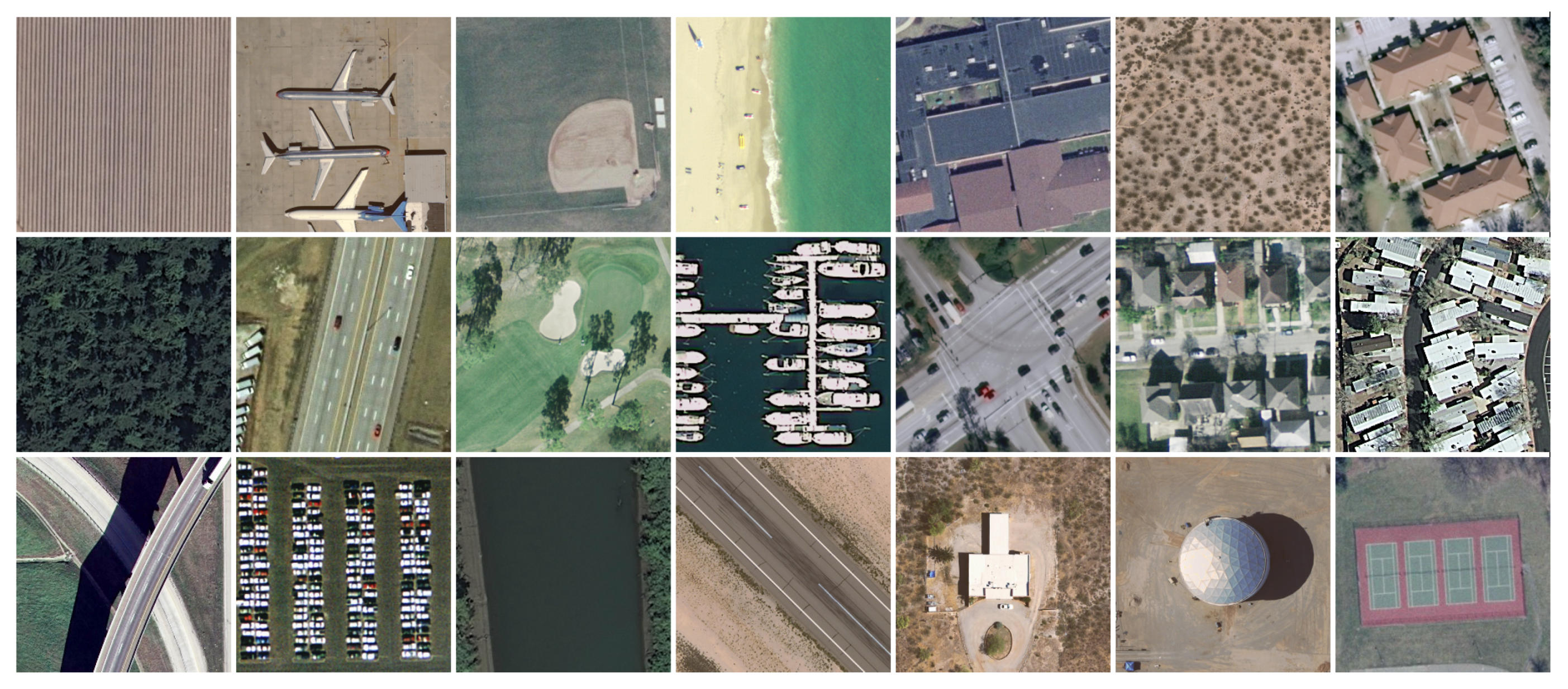
Area imagery data processing plays a key role in many remote sensing applications, such as land-use mapping [49]. We adopt the popular area imagery dataset UCMerced [50], which is a 21 class land use image dataset meant for research purposes. The images were manually extracted from large images from the USGS National Map Urban Area Imagery collection for various urban areas around the country. The pixel resolution of this public domain imagery is 1 foot, and each RGB image measures pixels. There are 100 images for each class, and we chose the 85-th image to form a dataset of 21 images as shown in Figure 4.
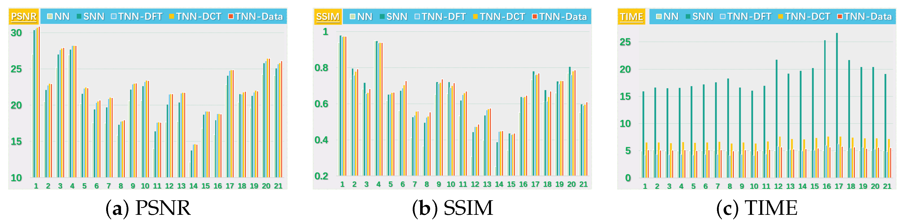
We consider two scenarios by setting for the images. For NN (Model (32)), we set the regularization parameters (suggested by [38]), and tune the parameter around (suggested by [51]). For SNN, the parameter is tuned in for better performance in most cases, and the weight is set by . For Algorithm 1, we tune around , and let for TNN (DFT) and for TNN (DCT) and TNN (Data). In each setting, we test each image for 10 trials and report the averaged PSNR (in db), SSIM and running time (in seconds).
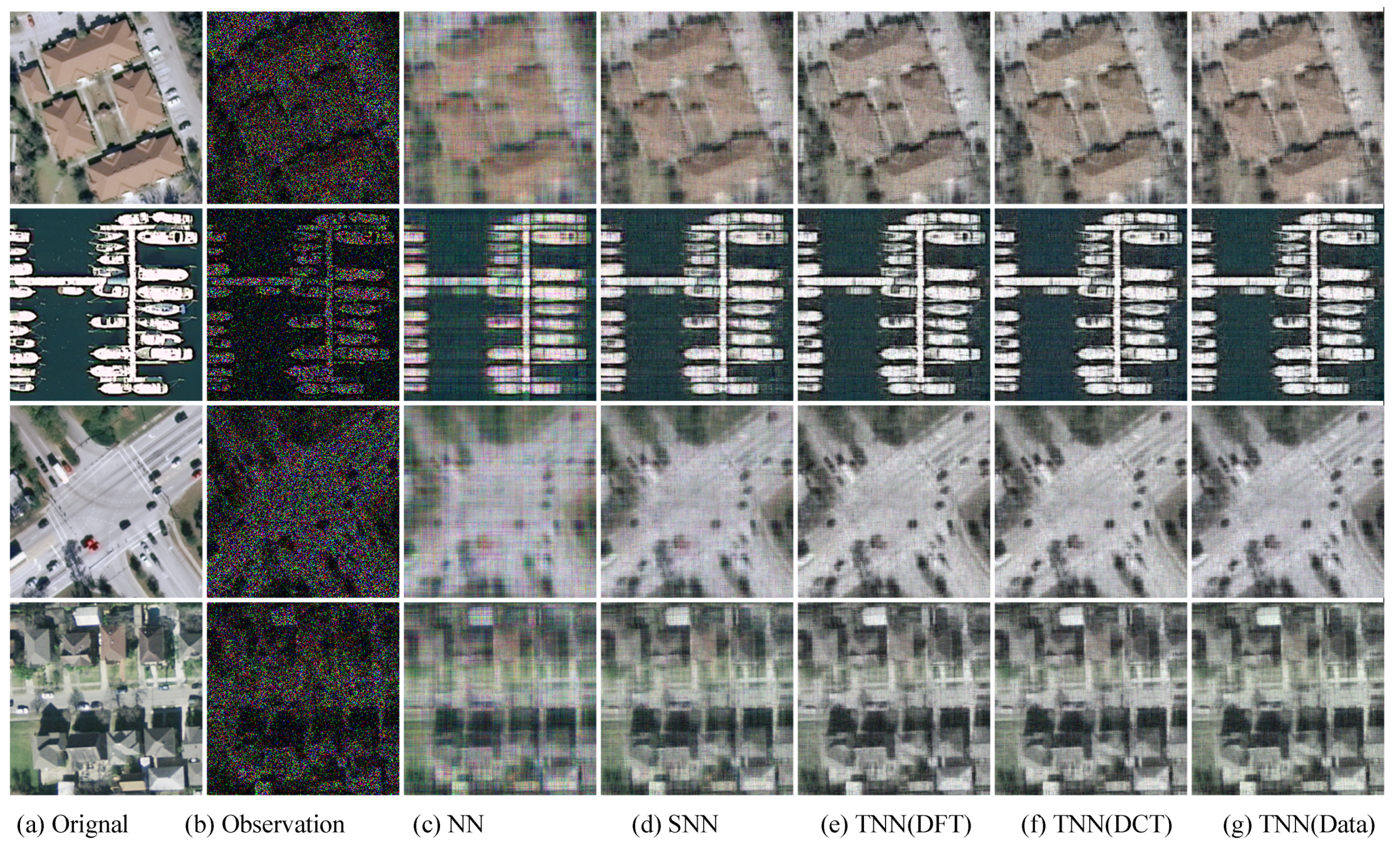
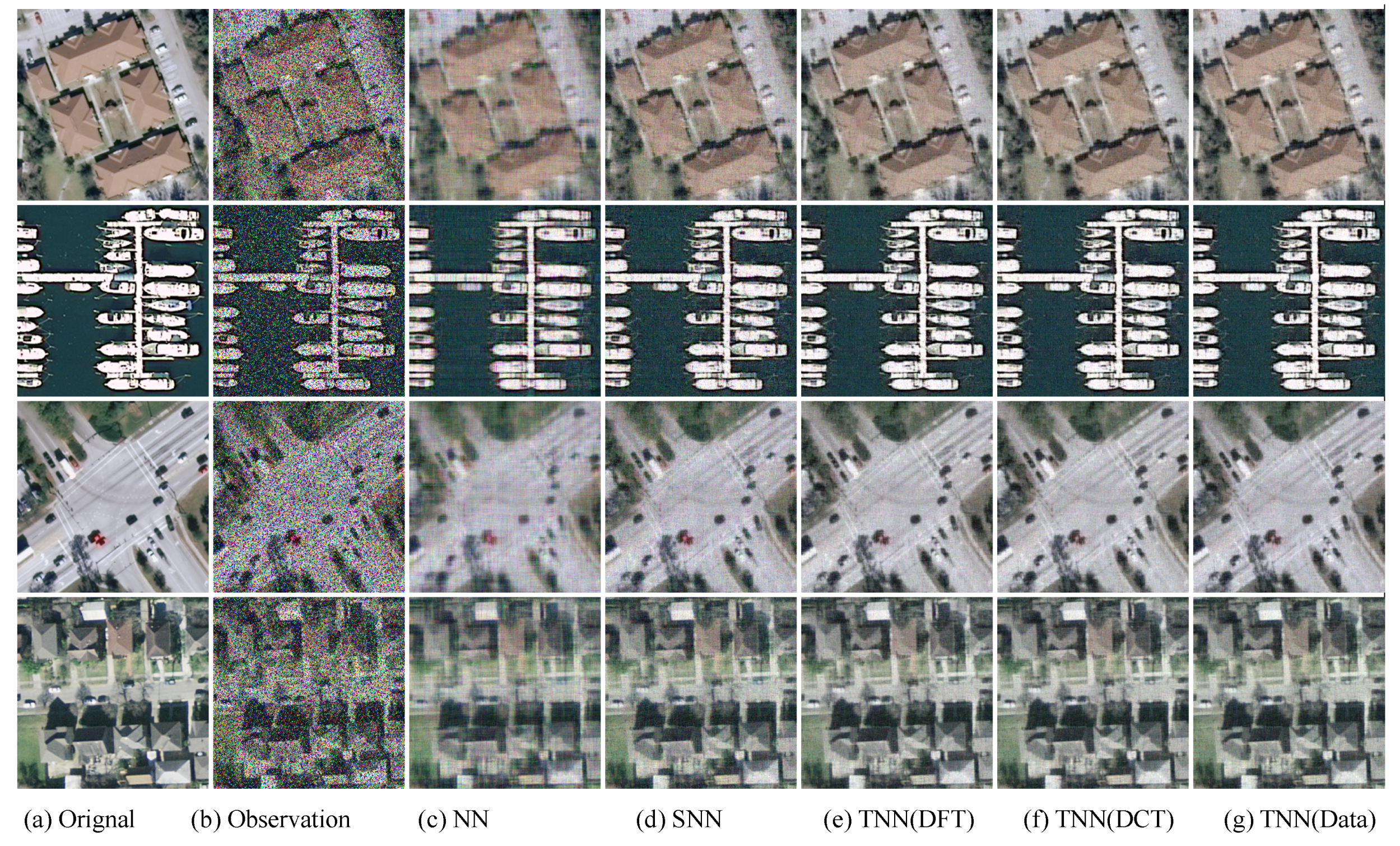
We present the PSNR, SSIM values and running time in Figure 5 and Figure 6 for settings of and , respectively, for quantitative evalution, with visual examples shown in Figure 7 and Figure 8. It can seen that from Figure 5, Figure 6, Figure 7 and Figure 8 that the proposed TNN (Data) has the highest recovery quality in most cases, and posses a comparative running time as NN. We attribute the promising performance of the proposed algorithm to the extraordinary representation power of the low-tubl-rank models: low-tubal-rankness can exploit both low-rankness and smoothness simultaneously, whereas traditional models like NN and SNN can only exploit low-rankness in the original domain [18].
7.2.2. Experiments on Hyperspectral Data
Benefit from its fine spectral and spatial resolutions, hyperspectral image processing has been extensively adopted in many remote sensing applications [10,52]. In this section, we conduct robust tensor completion on subsets of the two representative hyperspectral datasets described as follows:
- Indian Pines: This dataset was collected by AVIRIS sensor in 1992 over the Indian Pines test site in North-western Indiana and consists of pixels and 224 spectral reflectance bands. We use the first 30 bands in the experiments due to the trade-off between the limitation of computing resources and the efforts for parameter tuning.
- Salinas A: The data were acquired by AVIRIS sensor over the Salinas Valley, California in 1998, and consists of 224 bands over a spectrum range of 400–2500 nm. This dataset has a spatial extent of pixels with a resolution of 3.7 m. We use the first 30 bands in the experiments too.
We consider three settings, i.e., Setting I , , Setting II , , and Setting III for robust completion of hyper-spectral data. For NN, we set the regularization parameters (suggested by [38]), and tune the parameter around (suggested by [51]). For SNN, the parameter is tuned in for better performance in most cases, and we chose the weight by (suggested by [47]). For Algorithm 1, we tune the parameter around , and let for TNN (DFT) and for TNN (DCT) and TNN (Data). In each setting, we test each image for 10 trials and report the averaged PSNR (in db), SSIM and running time (in seconds).
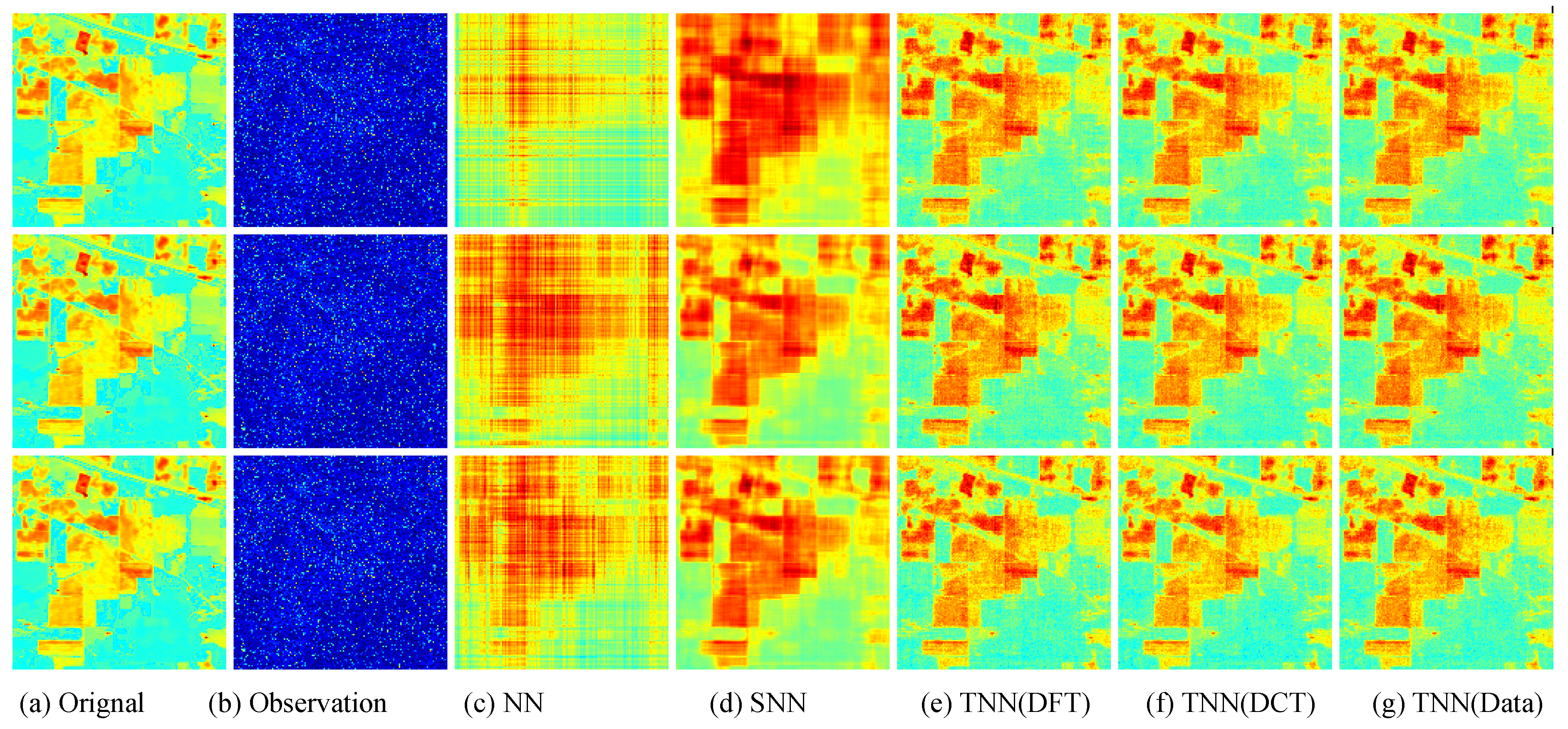
For quantitative evalution, we report the PSNR, SSIM values and running time in Table 2 and Table 3 for the Indian Pines and Salinas A datasets, respectively. The visual examples are, respectively, shown in Figure 9 and Figure 10. It can seen that the proposed TNN (Data) has the highest recovery quality in most cases, and has a comparative running time as NN, indicating the effectiveness and efficiency of low-tubal-rank models in comparison with original domain-based models NN and SNN.
7.2.3. Experiments on Multispectral Images
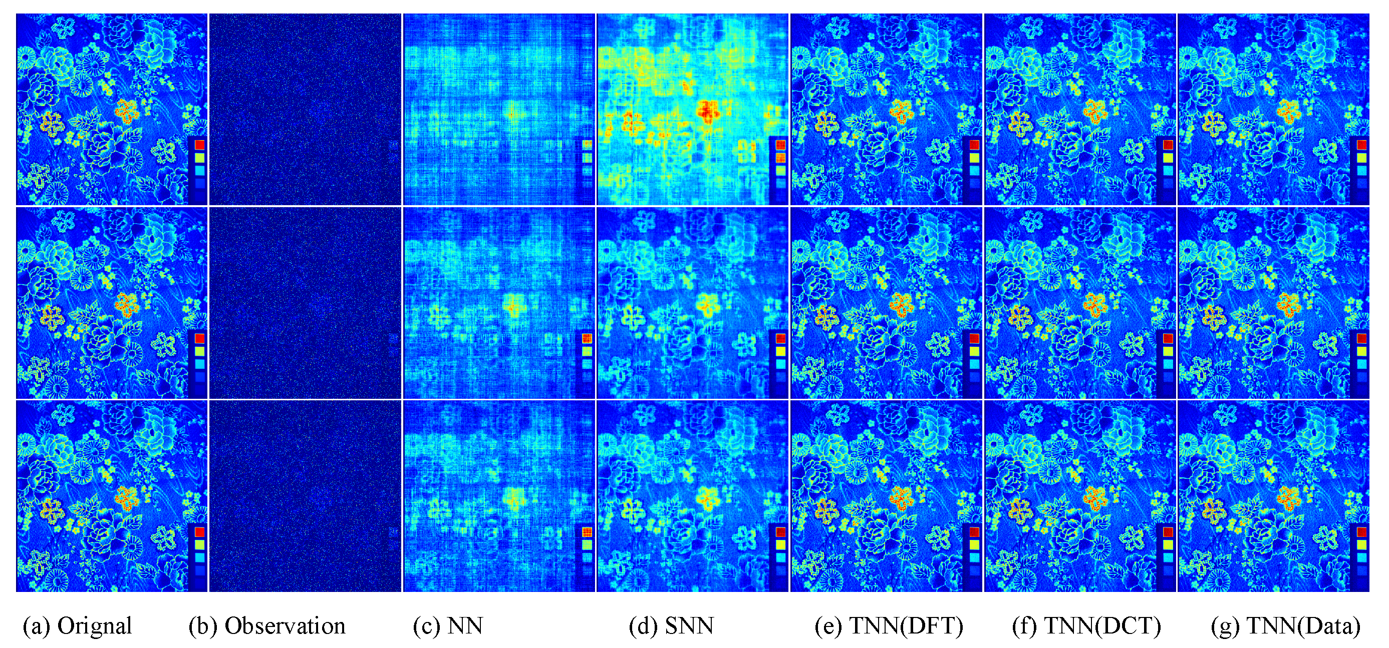
Multispectral imaging captures image data within specific wavelength ranges across the electromagnetic spectrum, and has become one of the most widely utilized datatype in remote sensing. This section presents simulated experiments on multispectral images. The original data are two multispectral images Beads and Cloth from the Columbia MSI Database (available at http://www1.cs.columbia.edu/CAVE/databases/multispectral accessed on 28 July 2021) containing scenes of a variety of real-world objects. Each MSI is of size 512 × 512 × 31 with intensity range scaled to [0, 1].
We also consider three settings, i.e., Setting I , Setting II , and Setting III for robust completion of multi-spectral data. We tune the parameters in the same way as Section 7.2.2. In each setting, we test each image for 10 trials and report the averaged PSNR (in db), SSIM and running time (in seconds).
For quantitative evalution, we report the PSNR, SSIM values and running time in Table 4 and Table 5 for the Beads and Cloth datasets, respectively. The visual examples for the Cloth dataset is shown in Figure 11. We can also find that the proposed TNN (Data) achieves the highest accuracy in most cases, and has a comparative running time as NN, which demonstrates both the effectiveness and efficiency of low-tubal-rank models.
7.2.4. Experiments on Point Could Data
With the rapid advances of sensor technology, the emerging point cloud data provide better performance than 2D images in many remote sensing applications due to its flexible and scalable geometric representation [53]. In this section, we also conduct experiments on a dataset (scenario B from http://www.mrt.kit.edu/z/publ/download/velodynetracking/dataset.html, accessed on 28 July 2021) for Unmanned Ground Vehicle (UGV). The dataset contains a sequence of point cloud data acquired from a Velodyne HDL-64E LiDAR. We select 30 frames (Frame Nos. 65-94) from the data sequence. The point cloud data is formatted into two tensors sized representing the distance data (named SenerioB Distance) and the intensity data (named SenerioB Intensity), , respectively.
We also consider three settings, i.e., Setting I , Setting II , and Setting III for robust completion of point cloud data. We tune the parameters in the same way as Section 7.2.2. In each setting, we test each image for 10 trials and report the averaged PSNR (in db), SSIM and running time (in seconds). For quantitative evalution, we report the PSNR, SSIM values and running time in Table 6 and Table 7 for the SenerioB Distance and SenerioB Intensity datasets, respectively. We can also find that the proposed TNN (Data) achieves the highest accuracy in most cases, and has a comparative running time as NN, which demonstrates both the effectiveness and efficiency of low-tubal-rank models.
7.2.5. Experiments on Aerial Video Data
Aerial videos (or time sequences of images) are broadly used in many computer vision based remote sensing tasks [54]. We experiment on a tensor which consists of the first 30 frames of the Sky dataset (available at http://www.loujing.com/rss-small-target, accessed on 28 July 2021) for small object detection [55].
We also consider three settings, i.e., Setting I , Setting II , and Setting III . We tune the parameters in the same way as Section 7.2.2. In each setting, we test each image for 10 trials and report the averaged PSNR (in db), SSIM and running time (in seconds). For quantitative evalution, we report the PSNR, SSIM values and running time in Table 8. It is also found that the proposed TNN (Data) achieves the highest accuracy in most cases, and can run as fast as NN.
7.2.6. Experiments on Thermal Imaging Data
Thermal infrared data can provide important measurements of surface energy fluxes and temperatures in various remote sensing applications [7]. In this section, we experiment on two infrared datasets as follows:
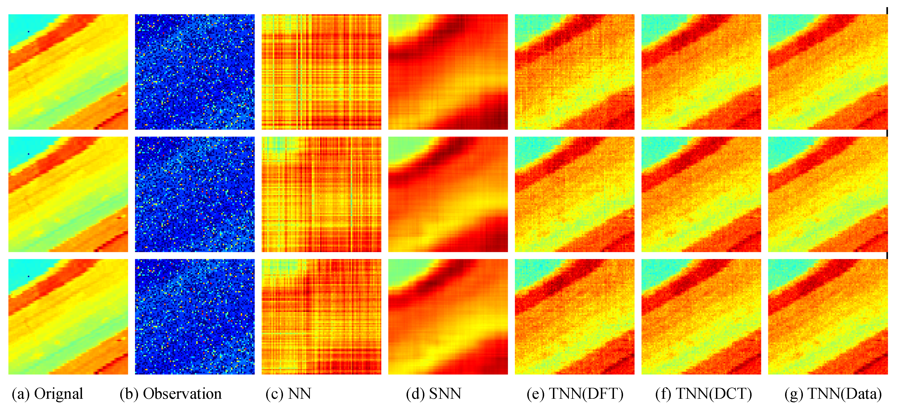
- The Infraed Detection dataset [56]: this dataset is collected for infrared detection and tracking of dim-small aircraft targets under ground/air background (available at http://www.csdata.org/p/387/, accessed on 28 July 2021). It consists of 22 subsets of infrared image sequences of all aircraft targets. We use the first 30 frames of data3.zip to form a tensor due to the trade-off between the limitation of computing resources and the efforts for parameter tuning.
- The OSU Thermal Database [3]: The sequences were recorded on the Ohio State University campus during the months of February and March 2005, and show several people, some in groups, moving through the scene. We use the first 30 frames of Sequences 1 and form a tensor of size .
Similiar to Section 7.2.2, we test in three settings, i.e., Setting I , Setting II , and Setting III , and use the same strategy for parameter tuning. In each setting, we test each image for 10 trials and report the averaged PSNR (in db), SSIM and running time (in seconds). For quantitative evalution, we report the PSNR, SSIM values and running time in Table 9 and Table 10 for the Infraed Detection and OSU Thermal Database datasets, respectively. The visual examples are, respectively, shown in Figure 12 and Figure 13. It can seen that the proposed TNN (Data) has the highest recovery quality in most cases, and has a comparative running time as NN, showing both effectiveness and efficiency of low-tubal-rank models in comparison with original domain-based models NN and SNN.
7.2.7. Experiments on SAR Data
Polarimetric synthetic aperture radar (PolSAR) has attracted lots of attention from remote sensing scientists because of its various advantages, e.g., all-weather, all-time, penetrating capability, and multi-polarimetry [57]. In this section, we adopt the PolSAR UAVSAR Change Detection Images dataset. It is a dataset of single-look quad-polarimetric SAR images acquired by the UAVSAR airborne sensor in L-band over an urban area in San Francisco city on 18 September 2009, and May 11, 2015. The dataset #1 have length and width of 200 pixels, and we use the first 30 bands.
We also consider three settings, i.e., Setting I , Setting II , and Setting III . We tune the parameters in the same way as Section 7.2.2. In each setting, we test each image for 10 trials and report the averaged PSNR (in db), SSIM and running time (in seconds) in Table 11. It is also found that the proposed TNN (Data) achieves the highest accuracy in most cases, and can run as fast as NN.
8. Conclusions
In this paper, we resolve the challenging robust tensor completion problem by proposing a -SVD-based estimator to robustly reconstruct a low-rank tensor in the presence of missing values, gross outliers, and small noises simultaneously. Specifically, this work can be concluded in the following three aspects:
- (1)
- Algorithmically, we design an efficient algorithm within the framework of ADMM to efficiently compute the proposed estimator with guaranteed convergence behavior.
- (2)
- Statistically, we analyze the statistical performance of the proposed estimator by establishing a non-asymptotic upper bound on the estimation error. The proposed upper bound is further proved to be minimax optimal (up to a log factor).
- (3)
- Experimentally, the correctness of the upper bound is first validated through simulations on synthetic datasets. Then both effectiveness and efficiency of the proposed algorithm are demonstrated by extensive comparisons with state-of-the-art nuclear norm based models (i.e., NN and SNN) on seven different types of remote sensing data.
However, from a critical point of view, the proposed method has the following two limitations:
- (1)
- The orientational sensitivity of -SVD: Despite the promising empirical performance of the -SVD-based estimator, a typical defect of it is the orientation sensitivity owing to low-rankness strictly defined along the tubal orientation which makes it fail to simultaneously exploit transformed low-rankness in multiple orientations [19,58].
- (2)
- The difficulty in finding the optimal transform for -SVD: Although a direct use of fixed transforms (like DFT and DCT) may produce fairish empirical performance, it is still unclear how to find the best optimal transformation for any certain tensor when only partial and corrupted observations are available.
According to the above limitations, it is interesting to consider higher-order extensions of the proposed model in an orientation invariant way like [19] and discuss the statistical performance. It is also interesting to consider the data-dependent transformation learning like [31,59]. Another future direction is to consider more efficient solvers of Problem (8) using the factorization strategy or Frank–Wolfe method [47,60,61,62].
Author Contributions
Conceptualization, A.W. and Q.Z.; Data curation, Q.Z.; Formal analysis, G.Z.; Funding acquisition, A.W., G.Z. and Q.Z.; Investigation, A.W.; Methodology, G.Z.; Project administration, A.W. and Q.Z.; Resources, Q.Z.; Software, A.W.; Supervision, G.Z. and Q.Z.; Validation, A.W., G.Z. and Q.Z.; Visualization, Q.Z.; Writing—original draft, A.W. and G.Z.; Writing—review & editing, A.W., G.Z. and Q.Z. All authors have read and agreed to the published version of the manuscript.
Funding
This work was supported in part by the National Natural Science Foundation of China under Grants 61872188, 62073087, 62071132, U191140003, 6197309, in part by the China Postdoctoral Science Foundation under Grant 2020M672536, in part by the Natural Science Foundation of Guangdong Province under Grants 2020A1515010671, 2019B010154002, 2019B010118001.
Institutional Review Board Statement
Not applicable.
Informed Consent Statement
Not applicable.
Data Availability Statement
In this paper, all the data supporting our experimental results are publicly available with references or URL links.
Acknowledgments
The authors are grateful to the editor and reviewers for their valuable time in processing this manuscript. The first author would like to thank Shasha Jin for her kind understanding in these months, and Zhong Jin in Nanjing University of Science and Technology for his long time support. The authors are also grateful to Xiongjun Zhang for sharing the code for [25] and Olga Klopp for her excellent theoretical analysis in [36,51] which is so helpful.
Conflicts of Interest
The authors declare no conflict of interest.
Appendix A. Proof of Theoretical Results
Appendix A.1. Additional Notations and Preliminaries
For the ease of exposition, we first list the additive notations often used in the proofs in Table A1.

Table A1.
Additional notations in the proofs.
| Notations | Descriptions | Notations | Descriptions |
|---|---|---|---|
| estimation error of | estimation error of | ||
| -tubal-rank of | sparsity of | ||
| inverse uncorrupted ratio | a | -norm bound in Equation (8) | |
| index set of design tensors corresponding to uncorrupted entries | |||
| index set of design tensors corresponding to corrupted entries | |||
| stochastic tensor defined to lower bound parameters and | |||
| stochastic tensor defined to lower bound parameter | |||
| random tensor defined in bounding with i.i.d. Rademacher | |||
| expectation of for defined to establish the RSC condition | |||
We then introduce the decomposability of -TNN and tensor -norm which plays a key role in the analysis.
Decomposability of -TNN. Suppose has reduced -SVD as , where and are orthogonal and is f-diagonal. Define projectors and as follows:
Then, it can be verified that:
- (I).
- , ;
- (II).
- , .
- (III).
- , .
In the same way to the results in supplementary material of [43], it can also be shown that the following equations hold:
- (I).
- (Decomposability of –TNN) For any satisfying , ,
- (II).
- (Norm compatibility inequality) For any
Decomposability of tensor -norm [63]. Let denote any index set and its complement. Then for any tensor , define two tensors and as follows
Then, one has
- (I).
- (Decomposability of -norm) For any ,
- (II).
- (Norm compatibility inequality) For any ,
Appendix A.2. The Proof for Theorem 3
The proof follows the lines of [34,36]. For notational simplicity, we define the following two sets
which denote the index set of design tensors corresponding to uncorrupted/corrupted entries, respectively.
Appendix A.2.1. Mainstream of Proving Theorem 3
Proof of Theorem 3.
Equation (A5) indicates that
which leads to
where , and the equality holds. Now each item in the right hand side of (A8) will be upper bounded separately as follows. Following the idea of [36], the upper bound will be analyzed upon the following event
According to the tail behavior of the maximum in a sub-Gaussian sequence, it holds with an absolute constant such that .
Bound. On the event , we get
Bound. Note that according to the properties of -TNN, we have
Thus, we can bound term by
By letting , it holds that
Bound: Note that since , we have , leading to
Letting yields
Then, we follow the line of [36] to specify a kind of Restricted Strong Convexity (RSC) for the random sampling operator formed by the design tensors on a carefully chosen constrained set. The RSC will show that when the error tensors belong to the constrained set, the following relationship:
holds with an appropriate residual with high probability.
Before explicitly defining the constrained set, we first consider the following set where should lie:
with two positive constants and whose values will be specified later. We also define the following set of tensor pairs:
We then define the constrained set as the intersection:
To bound the estimation error in Equation (26), we will upper bound and separately.
Note that
and similarly
We will bound and separately. We first bound in what follows.
Case 1: If , then we use the following inequality
which holds due to .
Thus, we can upper bound with an upper bound of in Lemma A1
Case 2: Suppose . First, according to Lemma A3, it holds on the event defined in Equation (A9) that
where holds due to the triangular inequality; is a direct consequence of Lemma A3, and the definition of event ; holds because , and for any ; stems from the inequality ; is due to the triangular inequality; holds since .
Note that according to Lemma A1, we have with probability at least :
where is defined in Lemma A4.
Then, according to Lemma A6, it holds with probability at least that
where is defined in Equation (A64).
Recall that Equation (A13) writes:
Letting , we further obtain
Note that the bound on is given in Lemma A4, and the values of and can be set according to Lemmas A8 and A9, respectively. Then, by putting Equations (A18), (A19) and (A52) together, and using Lemmas A8 and A9 to bound associated norms of the stochastic quantities , , and in the error term, we can obtain the bound on and complete the proof. □
Appendix A.2.2. Lemmas for the Proof of Theorem 3
Lemma A1.
Letting , it holds that
Proof of Lemma A1.
By the standard condition for optimality over a convex set, it holds that for any feasible
which further leads to
Letting , we have
Note that
Thus, we have
One the other hand, the definition of sub-differential indicates
which implies
Also note that
which implies
Since , we have
Thus, it holds that
which complete the proof. □
Lemma A2.
It holds that
Proof of Lemma A2.
Note that
where hold since is the dual norm of ; holds since and the tensor -norm is invariant to changes in sign. □
Lemma A3.
By letting and , we have
Proof of Lemma A3.
In Equation (A33), letting , we obtain
First, note that
Also, we have according to the convexity of and that
Thus, we have
Moreover, it is often used that
Since we set and , we have
where we use . It implies
Note that, . Thus, we have
□
Lemma A4.
If and , then on the event defined in Equation (A9), we have
and it holds with probability at least that
Proof of Lemma A4.
(I) The proof of Equation (A51): Recall that Lemma A1 implies
Then, we have on event :
where holds due to Assumption A1.I; is a direct use of Lemma A1; stems from the facts that and the definition of event in Equation (A9).
Thus, Equation (A51) is proved.
(II) The proof of Equation (A52): According to the optimality of to Problem (8), we have
which implies
which further leads to
Note that by using , we have
Thus on the event defined in Equation (A9), we have
where holds due to Lemma A2; holds because , and ; holds because , and ; holds as a consequence of , (due to Assumption A1.I), and the definition of event .
Now, we discuss the bound of in two cases.
□
Lemma A5.
Define the following set
Then, it holds with probability at least that
for any .
Proof of Lemma A5.
We prove this lemma using a standard peeling argument. First, define the following
We partition this set to simpler events with :
Note that according to Lemma A7, we have with :
Thus, we have
where is due to for positive x. By setting and recalling the value of , the lemma is proved. □
Lemma A6.
For any , it holds with probability at least that
where
Proof of Lemma A6.
The proof is very similar to that of Lemma A5, and we simply omit it. □
Lemma A7.
Define the set
and
Then, it holds that
Proof of Lemma A7.
First, we study the tail behavior of by directly using the Massart’s inequality in Theorem 14.2 of [64]. According to the Massart’s inequality, it holds for any
By letting , the first inequality in Equation (A67) is proved.
Then, we will upper bound the expectation of . By standard symmetrization argument [65], we have
where ’s are i.i.d. Randemacher variables. Further, according to the contraction principle [66], it holds that
In the following, we consider the two cases:
Case 1. Consider , we have
By letting in Equation (A68), we obtain
when .
Case 2. Consider , where , , and . The goal in this case is to upper bound
where holds as a property of the sup operation; holds due to the definition of dual norm; stems from the condition .
It remains to upper bound in Equation (A72). First, according to the definition of , we have
We also have
where holds due to the triangular inequality, and is a result of conditions and . Since Assumption A1.II indicates , combing Equations (A74) and (A75) further yields an upper bound on as follows:
which further leads to
The application of is also used to further relax the above inequality:
Lemma A8.
Under Assumption A1, there exists an absolute constant such that the following bounds on the tensor spectral norm of stochastic tensors and hold:
- (I)
- For tensor , we have
- (II)
- For tensor , we have
Proof of Lemma A8.
Lemma A9.
Under Assumption A1, there exists an absolute constant such that the following bounds on the -norm of stochastic tensors , , and hold:
- (I)
- For tensor , we have
- (II)
- For tensor , we have
- (III)
- For tensor , we have
Proof of Lemma A9.
Since this lemma can be straightforwardly proved in the same way as Lemma 10 in [36], we omit the proof. □
Appendix A.3. Proof of Theorem 4
The proof of Theorem 4 follows those of Theorems 2 and 3 in [36] for robust matrix completion. Given and , let be the probability with respect to the random design tensors and random noises according to the observation model in Equation (6). Without loss of generality, we assume .
Proof of Theorem 4.
For element-wisely sparse , we first construct a set which satisfies the following conditions:
- (i)
- For any tensor in , we have ;
- (ii)
- For any two tensors in , we have ;
- (iii)
- For any tensor in , any of its entries are in , where ,
Motivated by the proof of Theorem 2 in [36], is constructed as follows
where is the zero matrix, and with being a small enough constant such that .
Next, according to the Varshamov-Gilbert lemma (see Lemma 2.9 in [67]), there exists a set containing the zero tensor , such that
- (i)
- its cardinality , and
- (ii)
- for any two distinct tensors and in ,
Let denote the probabilistic distribution of random variables observed when the underlying tensor is in the observation model (6). Note that, the distribution of the random noise . Thus, for any , the KL divergence between and satisfies
Hence, if we choose , then it holds that
for any .
According to Theorem 2.5 in [67], using Equations (A88) and (A90), there exists a constant , such that
where
Note that b can be chosen to be arbitrarily small, then low-rank part of Theorem 4 is proved.
Then, we consider the sparse part of Theorem 4. Given a set with cardinality , we also define as follows
where is the zero tensor, and . Then, according to the Varshamov-Gilbert lemma (see Lemma 2.9 in [67]), there exists a set containing the zero tensor , such that: (i) its cardinality , and (ii) for any two distinct tensors and in ,
Let denote the probabilistic distribution of random variables observed when the underlying tensor is in the observation model (6). Thus, for any , the KL divergence between and satisfies
Hence, if we choose , then it holds that
for any . According to Theorem 2.5 in [67], using Equations (A93) and (A95), there exists a constant , such that
where
Note that can be chosen to be arbitrarily small, then sparse part of Theorem 4 is proved.
Thus, according to Equations (A91) and (A96), by setting
the following relationship holds
where . Then according to Markov inequality, we obtain
□
References
- He, W.; Yokoya, N.; Yuan, L.; Zhao, Q. Remote sensing image reconstruction using tensor ring completion and total variation. IEEE Trans. Geosci. Remote Sens. 2019, 57, 8998–9009. [Google Scholar] [CrossRef]
- He, W.; Yao, Q.; Li, C.; Yokoya, N.; Zhao, Q.; Zhang, H.; Zhang, L. Non-local meets global: An integrated paradigm for hyperspectral image restoration. IEEE Trans. Pattern Anal. Mach. Intell. 2020. [Google Scholar] [CrossRef] [PubMed]
- Davis, J.W.; Sharma, V. Background-subtraction using contour-based fusion of thermal and visible imagery. Comput. Vis. Image Underst. 2007, 106, 162–182. [Google Scholar] [CrossRef]
- Bello, S.A.; Yu, S.; Wang, C.; Adam, J.M.; Li, J. Deep learning on 3D point clouds. Remote Sens. 2020, 12, 1729. [Google Scholar] [CrossRef]
- Zheng, Y.B.; Huang, T.Z.; Zhao, X.L.; Chen, Y.; He, W. Double-factor-regularized low-rank tensor factorization for mixed noise removal in hyperspectral image. IEEE Trans. Geosci. Remote Sens. 2020, 58, 8450–8464. [Google Scholar] [CrossRef]
- Liu, H.K.; Zhang, L.; Huang, H. Small target detection in infrared videos based on spatio-temporal tensor model. IEEE Trans. Geosci. Remote Sens. 2020, 58, 8689–8700. [Google Scholar] [CrossRef]
- Zhou, A.; Xie, W.; Pei, J. Background modeling combined with multiple features in the Fourier domain for maritime infrared target detection. IEEE Trans. Geosci. Remote. Sens. 2021. [Google Scholar] [CrossRef]
- Jiang, Q.; Ng, M. Robust low-tubal-rank tensor completion via convex optimization. In Proceedings of the 28th International Joint Conference on Artificial Intelligence, Macao, China, 10–16 August 2019; AAAI Press: Palo Alto, CA, USA, 2019; pp. 2649–2655. [Google Scholar]
- Zhao, Q.; Zhou, G.; Zhang, L.; Cichocki, A.; Amari, S.I. Bayesian robust tensor factorization for incomplete multiway data. IEEE Trans. Neural Networks Learn. Syst. 2016, 27, 736–748. [Google Scholar] [CrossRef] [Green Version]
- Liu, H.; Li, H.; Wu, Z.; Wei, Z. Hyperspectral image recovery using non-convex low-rank tensor approximation. Remote Sens. 2020, 12, 2264. [Google Scholar] [CrossRef]
- Ma, T.H.; Xu, Z.; Meng, D. Remote sensing image denoising via low-rank tensor approximation and robust noise modeling. Remote Sens. 2020, 12, 1278. [Google Scholar] [CrossRef] [Green Version]
- Fazel, M. Matrix Rank Minimization with Applications. Ph.D. Thesis, Stanford University, Stanford, CA, USA, 2002. [Google Scholar]
- Liu, J.; Musialski, P.; Wonka, P.; Ye, J. Tensor completion for estimating missing values in visual data. IEEE Trans. Pattern Anal. Mach. Intell. 2013, 35, 208–220. [Google Scholar] [CrossRef]
- Carroll, J.D.; Chang, J. Analysis of individual differences in multidimensional scaling via an N-way generalization of “Eckart-Youn” decomposition. Psychometrika 1970, 35, 283–319. [Google Scholar] [CrossRef]
- Tucker, L.R. Some mathematical notes on three-mode factor analysis. Psychometrika 1966, 31, 279–311. [Google Scholar] [CrossRef] [PubMed]
- Oseledets, I. Tensor-train decomposition. SIAM J. Sci. Comput. 2011, 33, 2295–2317. [Google Scholar] [CrossRef]
- Zhao, Q.; Zhou, G.; Xie, S.; Zhang, L.; Cichocki, A. Tensor ring decomposition. arXiv 2016, arXiv:1606.05535. [Google Scholar]
- Wang, A.; Zhou, G.; Jin, Z.; Zhao, Q. Tensor recovery via *L-spectral k-support norm. IEEE J. Sel. Top. Signal Process. 2021, 15, 522–534. [Google Scholar] [CrossRef]
- Wang, A.; Li, C.; Jin, Z.; Zhao, Q. Robust tensor decomposition via orientation invariant tubal nuclear norms. In Proceedings of the The AAAI Conference on Artificial Intelligence (AAAI), New York, NY, USA, 7–12 February 2020; pp. 6102–6109. [Google Scholar]
- Zhang, Z.; Ely, G.; Aeron, S.; Hao, N.; Kilmer, M. Novel methods for multilinear data completion and de-noising based on tensor-SVD. In Proceedings of the IEEE Conference on Computer Vision and Pattern Recognition (CVPR), Columbus, OH, USA, 23–28 June 2014; pp. 3842–3849. [Google Scholar]
- Liu, X.; Aeron, S.; Aggarwal, V.; Wang, X. Low-tubal-rank tensor completion using alternating minimization. IEEE Trans. Inf. Theory 2020, 66, 1714–1737. [Google Scholar] [CrossRef]
- Kilmer, M.E.; Braman, K.; Hao, N.; Hoover, R.C. Third-order tensors as operators on matrices: A theoretical and computational framework with applications in imaging. SIAM J. Matrix Anal. A 2013, 34, 148–172. [Google Scholar] [CrossRef] [Green Version]
- Liu, X.Y.; Wang, X. Fourth-order tensors with multidimensional discrete transforms. arXiv 2017, arXiv:1705.01576. [Google Scholar]
- Kernfeld, E.; Kilmer, M.; Aeron, S. Tensor–tensor products with invertible linear transforms. Linear Algebra Its Appl. 2015, 485, 545–570. [Google Scholar] [CrossRef]
- Zhang, X.; Ng, M.K.P. Low rank tensor completion with poisson observations. IEEE Trans. Pattern Anal. Mach. Intell.. 2021. [Google Scholar] [CrossRef]
- Lu, C.; Peng, X.; Wei, Y. Low-rank tensor completion with a new tensor nuclear norm induced by invertible linear transforms. In Proceedings of the IEEE Conference on Computer Vision and Pattern Recognition (CVPR), Long Beach, CA, USA, 16–20 June 2019; pp. 5996–6004. [Google Scholar]
- Song, G.; Ng, M.K.; Zhang, X. Robust tensor completion using transformed tensor singular value decomposition. Numer. Linear Algebr. 2020, 27, e2299. [Google Scholar] [CrossRef]
- He, B.; Yuan, X. On the O(1/n) convergence rate of the Douglas–Rachford alternating direction method. SIAM J. Numer. Anal. 2012, 50, 700–709. [Google Scholar] [CrossRef]
- Parikh, N.; Boyd, S. Proximal algorithms. Found. Trends® Optim. 2014, 1, 127–239. [Google Scholar] [CrossRef]
- Kolda, T.G.; Bader, B.W. Tensor decompositions and applications. SIAM Rev. 2009, 51, 455–500. [Google Scholar] [CrossRef]
- Kong, H.; Lu, C.; Lin, Z. Tensor Q-rank: New data dependent definition of tensor rank. Mach. Learn. 2021, 110, 1867–1900. [Google Scholar] [CrossRef]
- Lu, C.; Zhou, P. Exact recovery of tensor robust principal component analysis under linear transforms. arXiv 2019, arXiv:1907.08288. [Google Scholar]
- Zhang, Z.; Aeron, S. Exact tensor completion using t-SVD. IEEE Trans. Signal Process. 2017, 65, 1511–1526. [Google Scholar] [CrossRef]
- Wang, A.; Jin, Z.; Tang, G. Robust tensor decomposition via t-SVD: Near-optimal statistical guarantee and scalable algorithms. Signal Process. 2020, 167, 107319. [Google Scholar] [CrossRef]
- Zhou, P.; Feng, J. Outlier-robust tensor PCA. In Proceedings of the IEEE Conference on Computer Vision and Pattern Recognition, Honolulu, HI, USA, 21–26 July 2017. [Google Scholar]
- Klopp, O.; Lounici, K.; Tsybakov, A.B. Robust matrix completion. Probab. Theory Relat. Fields 2017, 169, 523–564. [Google Scholar] [CrossRef]
- Lu, C.; Feng, J.; Chen, Y.; Liu, W.; Lin, Z.; Yan, S. Tensor robust principal component analysis: Exact recovery of corrupted low-rank tensors via convex optimization. In Proceedings of the IEEE Conference on Computer Vision and Pattern Recognition (CVPR), Las Vegas, NV, USA, 26 June–1 July 2016; pp. 5249–5257. [Google Scholar]
- Candès, E.J.; Li, X.; Ma, Y.; Wright, J. Robust principal component analysis? J. ACM (JACM) 2011, 58, 11. [Google Scholar] [CrossRef]
- Negahban, S.; Wainwright, M.J. Estimation of (near) low-rank matrices with noise and high-dimensional scaling. Ann. Stat. 2011, 39, 1069–1097. [Google Scholar] [CrossRef]
- Wang, A.; Wei, D.; Wang, B.; Jin, Z. Noisy low-tubal-rank tensor completion through iterative singular tube thresholding. IEEE Access 2018, 6, 35112–35128. [Google Scholar] [CrossRef]
- Boyd, S.; Parikh, N.; Chu, E. Distributed optimization and statistical learning via the alternating direction method of multipliers. Found. Trends® Mach. Learn. 2011, 3, 1–122. [Google Scholar]
- Wang, A.; Jin, Z. Near-optimal noisy low-tubal-rank tensor completion via singular tube thresholding. In Proceedings of the IEEE International Conference on Data Mining Workshop (ICDMW), New Orleans, LA, USA, 18–21 November 2017; pp. 553–560. [Google Scholar]
- Wang, A.; Lai, Z.; Jin, Z. Noisy low-tubal-rank tensor completion. Neurocomputing 2019, 330, 267–279. [Google Scholar] [CrossRef]
- Wang, A.; Song, X.; Wu, X.; Lai, Z.; Jin, Z. Generalized Dantzig selector for low-tubal-rank tensor recovery. In Proceedings of the The International Conference on Acoustics, Speech, and Signal Processing (ICASSP), Brighton, UK, 12–17 May 2019; pp. 3427–3431. [Google Scholar]
- Huang, B.; Mu, C.; Goldfarb, D.; Wright, J. Provable models for robust low-rank tensor completion. Pac. J. Optim. 2015, 11, 339–364. [Google Scholar]
- Wang, A.; Song, X.; Wu, X.; Lai, Z.; Jin, Z. Robust low-tubal-rank tensor completion. In Proceedings of the ICASSP 2019-2019 IEEE International Conference on Acoustics, Speech and Signal Processing (ICASSP), Brighton, UK, 12–17 May 2019; pp. 3432–3436. [Google Scholar]
- Fang, W.; Wei, D.; Zhang, R. Stable tensor principal component pursuit: Error bounds and efficient algorithms. Sensors 2019, 19, 5335. [Google Scholar] [CrossRef] [Green Version]
- Wang, Z.; Bovik, A.C.; Sheikh, H.R.; Simoncelli, E.P. Image quality assessment: From error visibility to structural similarity. IEEE Trans. Image Process. 2004, 13, 600–612. [Google Scholar] [CrossRef] [Green Version]
- Chen, J.; Wang, C.; Ma, Z.; Chen, J.; He, D.; Ackland, S. Remote sensing scene classification based on convolutional neural networks pre-trained using attention-guided sparse filters. Remote Sens. 2018, 10, 290. [Google Scholar] [CrossRef] [Green Version]
- Yang, Y.; Newsam, S. Bag-of-visual-words and spatial extensions for land-use classification. In Proceedings of the 18th SIGSPATIAL International Conference on Advances in Geographic Information Systems, San Jose, CA, USA, 2–5 November 2010; pp. 270–279. [Google Scholar]
- Klopp, O. Noisy low-rank matrix completion with general sampling distribution. Bernoulli 2014, 20, 282–303. [Google Scholar] [CrossRef] [Green Version]
- Li, N.; Zhou, D.; Shi, J.; Wu, T.; Gong, M. Spectral-locational-spatial manifold learning for hyperspectral images dimensionality reduction. Remote Sens. 2021, 13, 2752. [Google Scholar] [CrossRef]
- Mayalu, A.; Kochersberger, K.; Jenkins, B.; Malassenet, F. Lidar data reduction for unmanned systems navigation in urban canyon. Remote Sens. 2020, 12, 1724. [Google Scholar] [CrossRef]
- Hwang, Y.S.; Schlüter, S.; Park, S.I.; Um, J.S. Comparative evaluation of mapping accuracy between UAV video versus photo mosaic for the scattered urban photovoltaic panel. Remote Sens. 2021, 13, 2745. [Google Scholar] [CrossRef]
- Lou, J.; Zhu, W.; Wang, H.; Ren, M. Small target detection combining regional stability and saliency in a color image. Multimed. Tools Appl. 2017, 76, 14781–14798. [Google Scholar] [CrossRef]
- Hui, B.; Song, Z.; Fan, H. A dataset for infrared detection and tracking of dim-small aircraft targets under ground/air background. China Sci. Data 2020, 5, 291–302. [Google Scholar]
- Wang, Z.; Zeng, Q.; Jiao, J. An adaptive decomposition approach with dipole aggregation model for polarimetric SAR data. Remote Sens. 2021, 13, 2583. [Google Scholar] [CrossRef]
- Wei, D.; Wang, A.; Feng, X.; Wang, B.; Wang, B. Tensor completion based on triple tubal nuclear norm. Algorithms 2018, 11, 94. [Google Scholar] [CrossRef] [Green Version]
- Han, X.; Wu, B.; Shou, Z.; Liu, X.Y.; Zhang, Y.; Kong, L. Tensor FISTA-net for real-time snapshot compressive imaging. In Proceedings of the AAAI Conference on Artificial Intelligence, New York, NY, USA, 7–12 February 2020; Volume 34, pp. 10933–10940. [Google Scholar]
- Mu, C.; Zhang, Y.; Wright, J.; Goldfarb, D. Scalable robust matrix recovery: Frank–Wolfe meets proximal methods. SIAM J. Sci. Comput. 2016, 38, A3291–A3317. [Google Scholar] [CrossRef] [Green Version]
- Wang, A.; Jin, Z.; Yang, J. A faster tensor robust PCA via tensor factorization. Int. J. Mach. Learn. Cybern. 2020, 11, 2771–2791. [Google Scholar] [CrossRef]
- Lou, J.; Cheung, Y. Robust Low-Rank Tensor Minimization via a New Tensor Spectral k-Support Norm. IEEE TIP 2019, 29, 2314–2327. [Google Scholar] [CrossRef] [PubMed]
- Negahban, S.; Yu, B.; Wainwright, M.J.; Ravikumar, P.K. A unified framework for high-dimensional analysis of M-estimators with decomposable regularizers. Proceedings of Advances in Neural Information Processing Systems, Vancouver, BC, USA, 7–10 December 2009; pp. 1348–1356. [Google Scholar]
- Bühlmann, P.; Van De Geer, S. Statistics for High-Dimensional Data: Methods, Theory and Applications; Springer Science & Business Media: Berlin/Heidelberg, Germany, 2011. [Google Scholar]
- Vershynin, R. High-Dimensional Probability: An Introduction with Applications in Data Science; Cambridge University Press: Cambridge, UK, 2018; Volume 47. [Google Scholar]
- Talagrand, M. A new look at independence. Ann. Probab. 1996, 24, 1–34. [Google Scholar] [CrossRef]
- Tsybakov, A.B. Introduction to Nonparametric Estimation; Springer: New York, NY, USA, 2011. [Google Scholar]
Figure 1.
An illustration of –SVD [18].
Figure 1.
An illustration of –SVD [18].

Figure 2.
An illustration of the robust tensor completion problem.

Figure 3.
Plots of the MSE versus the tubal rank of the underlying tensor, the number of corruptions , the number of uncorrupted observations and its inversion : (a) MSE vs. the tubal rank with fixed corruption level and number of uncorrupted observations ; (b) MSE vs. the number of corruptions with fixed tubal rank 9 and total observation number ; (c) MSE vs. the number of uncorrupted observation with and corruption level ; (d) MSE vs. with and .
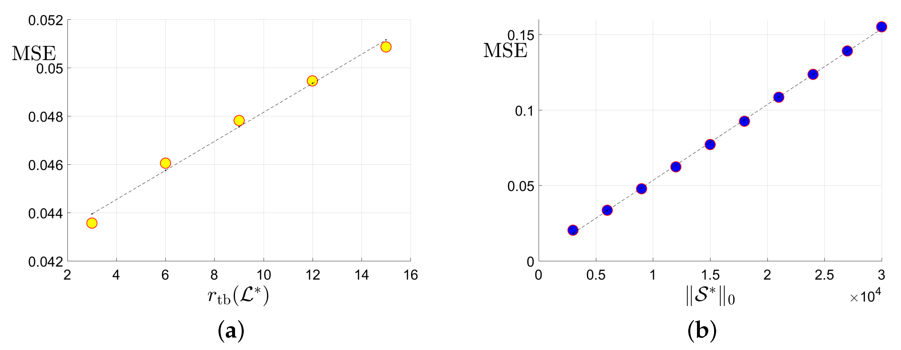

Figure 4.
The dataset consists of the 85-th frame of all the 21 classes in the UCMerced dataset.

Figure 5.
The PSNR, SSIM values and running time (in seconds) on the UCMerced dataset for the setting .
Figure 5.
The PSNR, SSIM values and running time (in seconds) on the UCMerced dataset for the setting .

Figure 6.
The PSNR, SSIM values and running time (in seconds) on the UCMerced dataset for the setting .
Figure 6.
The PSNR, SSIM values and running time (in seconds) on the UCMerced dataset for the setting .
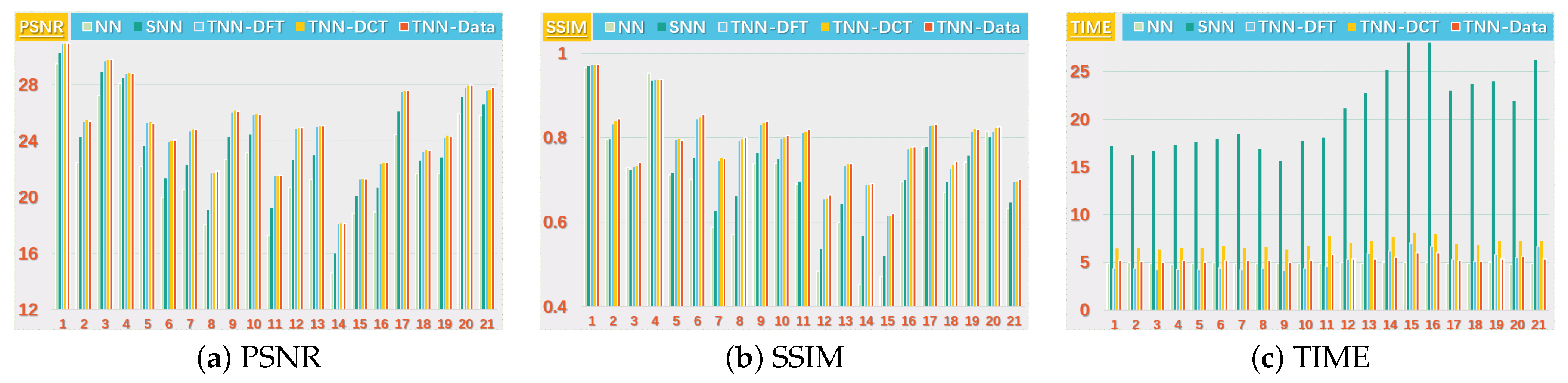
Figure 7.
The visual examples for five models on UCMerced dataset for the setting . (a) The original image; (b) the observed image; (c) image recovered by the matrix nuclear norm (NN) based Model (32); (d) recovered by the sum of mode-wise nuclear norms (SNN) based Model (33); (e) image recovered by TNN (DFT); (f) image recovered by TNN (DCT); (g) image recovered by TNN (Data).

Figure 8.
The visual examples for five models on UCMerced dataset for the setting . (a) The original image; (b) the observed image; (c) image recovered by the matrix nuclear norm (NN) based Model (32); (d) recovered by the sum of mode-wise nuclear norms (SNN) based Model (33); (e) image recovered by TNN (DFT); (f) image recovered by TNN (DCT); (g) image recovered by TNN (Data).

Figure 9.
Visual results of robust tensor completion for five models on the 21st bound of Indian Pines dataset. The top, middle, and bottum row corresponds to the Setting I , Setting II , and Setting III , respectively. The sub-plots from (a) to (g): (a) the original image; (b) the observed image; (c) image recovered by the matrix nuclear norm (NN) based Model (32); (d) recovered by the sum of mode-wise nuclear norms (SNN) based Model (33); (e) image recovered by TNN (DFT); (f) image recovered by TNN (DCT); (g) image recovered by TNN (Data).

Figure 10.
Visual results of robust tensor completion for five models on the 21st bound of Salinas A dataset. The top, middle, and bottum row corresponds to the Setting I , Setting II , and Setting III , respectively. The sub-plots from (a) to (g): (a) the original image; (b) the observed image; (c) image recovered by the matrix nuclear norm (NN) based Model (32); (d) recovered by the sum of mode-wise nuclear norms (SNN) based Model (33); (e) image recovered by TNN (DFT); (f) image recovered by TNN (DCT); (g) image recovered by TNN (Data).

Figure 11.
Visual results of robust tensor completion for five models on the 21st bound of Cloth dataset. The top, middle, and bottum row corresponds to the Setting I , Setting II , and Setting III , respectively. The sub-plots from (a) to (g): (a) The original image; (b) the observed image; (c) image recovered by the matrix nuclear norm (NN) based Model (32); (d) recovered by the sum of mode-wise nuclear norms (SNN) based Model (33); (e) image recovered by TNN (DFT); (f) image recovered by TNN (DCT); (g) image recovered by TNN (Data).

Figure 12.
Visual results of robust tensor completion for five models on the 21st bound of Infraed Detection dataset. The top, middle, and bottum row corresponds to the Setting I , Setting II , and Setting III , respectively. The sub-plots from (a) to (g): (a) the original image; (b) the observed image; (c) image recovered by the matrix nuclear norm (NN) based Model (32); (d) recovered by the sum of mode-wise nuclear norms (SNN) based Model (33); (e) image recovered by TNN (DFT); (f) image recovered by TNN (DCT); (g) image recovered by TNN (Data).
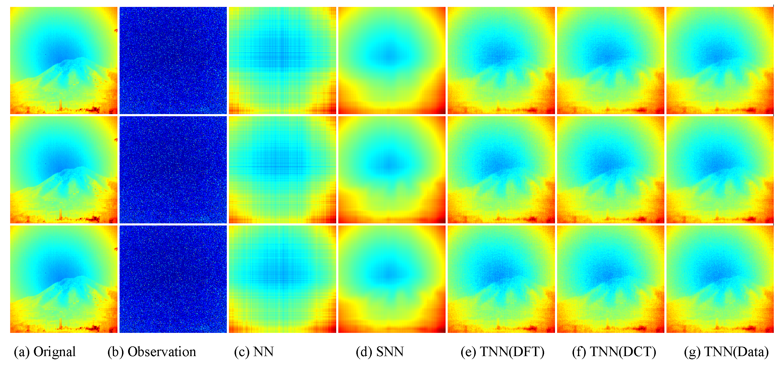
Figure 13.
Visual results of robust tensor completion for five models on the 21st bound of OSU Thermal Database dataset. The top, middle, and bottum row corresponds to the Setting I , Setting II , and Setting III , respectively. The sub-plots from (a) to (g): (a) the original image; (b) the observed image; (c) image recovered by the matrix nuclear norm (NN) based Model (32); (d) recovered by the sum of mode-wise nuclear norms (SNN) based Model (33); (e) image recovered by TNN (DFT); (f) image recovered by TNN (DCT); (g) image recovered by TNN (Data).

Table 1.
List of notations.
| Notations | Descriptions | Notations | Descriptions |
|---|---|---|---|
| t | a scaler | a matrix | |
| a vector | a tensor | ||
| the true low-rank tensor | the estimator of | ||
| the true sparse tensor | the estimator of | ||
| a scalar observation | Gaussian noise | ||
| a design tensor | N | number of observations | |
| number of uncorrupted observations | |||
| support of corruption tensor | complement of | ||
| design operator | adjoint operator of | ||
| an orthogonal matrix in | tensor L-transform | ||
| block-diagonal matrix of | tensor spectral norm | ||
| entry of | tubal nuclear norm | ||
| tube of | tensor -norm | ||
| frontal slice of | tensor F-norm | ||
| tensor -norm | |||
| mode-k unfolding of | tensor inner product |
Table 2.
Quantitative evaluation on the Indian Pines dataset in PSNR, SSIM, and running time of five models for robust tensor completion in three settings, i.e., Setting I , Setting II , and Setting III . The highest PSNR/SSIM, or lowest time (in seconds) is highlighted in bold.
Table 2.
Quantitative evaluation on the Indian Pines dataset in PSNR, SSIM, and running time of five models for robust tensor completion in three settings, i.e., Setting I , Setting II , and Setting III . The highest PSNR/SSIM, or lowest time (in seconds) is highlighted in bold.
| Settings | Metrics | NN | SNN | TNN-DFT | TNN-DCT | TNN-Data |
|---|---|---|---|---|---|---|
| PSNR | 20.63 | 25.46 | 28.49 | 29.33 | 30.08 | |
| Setting I | SSIM | 0.4842 | 0.7275 | 0.7619 | 0.7872 | 0.8181 |
| TIME | 14.77 | 40.1 | 11.17 | 15.53 | 13.54 | |
| PSNR | 21.95 | 27.66 | 29.49 | 30.17 | 30.61 | |
| Setting II | SSIM | 0.5454 | 0.7864 | 0.7912 | 0.8073 | 0.8296 |
| TIME | 14.18 | 39.76 | 11.04 | 15.23 | 13.29 | |
| PSNR | 22.43 | 28.22 | 29.64 | 30.31 | 30.87 | |
| Setting III | SSIM | 0.5534 | 0.8051 | 0.7971 | 0.8139 | 0.8345 |
| TIME | 14.21 | 38.88 | 11.05 | 15.27 | 13.43 |
Table 3.
Quantitative evaluation on the Salinas A dataset in PSNR, SSIM, and running time of five tensor completion models for robust tensor completion in three settings, i.e., Setting I , Setting II , and Setting III . The highest PSNR/SSIM, or lowest time (in seconds) is highlighted in bold.
Table 3.
Quantitative evaluation on the Salinas A dataset in PSNR, SSIM, and running time of five tensor completion models for robust tensor completion in three settings, i.e., Setting I , Setting II , and Setting III . The highest PSNR/SSIM, or lowest time (in seconds) is highlighted in bold.
| Settings | Metrics | NN | SNN | TNN-DFT | TNN-DCT | TNN-Data |
|---|---|---|---|---|---|---|
| PSNR | 19.01 | 26.18 | 27.1 | 30.99 | 32.69 | |
| Setting I | SSIM | 0.4918 | 0.837 | 0.7501 | 0.8350 | 0.8774 |
| TIME | 5.57 | 11.53 | 4.07 | 5.73 | 4.9 | |
| PSNR | 20.97 | 28.79 | 29.4 | 32.26 | 33.3 | |
| Setting II | SSIM | 0.5806 | 0.8675 | 0.8117 | 0.8645 | 0.8714 |
| TIME | 5.41 | 11.36 | 4.02 | 5.67 | 4.79 | |
| PSNR | 21.54 | 29.5 | 29.73 | 32.38 | 33.54 | |
| Setting III | SSIM | 0.5914 | 0.8772 | 0.8208 | 0.8683 | 0.8848 |
| TIME | 5.34 | 11.01 | 3.98 | 5.59 | 4.91 |
Table 4.
Quantitative evaluation on the Beads dataset in PSNR, SSIM, and running time of five tensor completion models for robust tensor completion in three settings, i.e., Setting I , Setting II , and Setting III . The highest PSNR/SSIM, or lowest time (in seconds) is highlighted in bold.
Table 4.
Quantitative evaluation on the Beads dataset in PSNR, SSIM, and running time of five tensor completion models for robust tensor completion in three settings, i.e., Setting I , Setting II , and Setting III . The highest PSNR/SSIM, or lowest time (in seconds) is highlighted in bold.
| Settings | Metrics | NN | SNN | TNN-DFT | TNN-DCT | TNN-Data |
|---|---|---|---|---|---|---|
| PSNR | 18.58 | 18.71 | 25.11 | 25.18 | 27.05 | |
| Setting I | SSIM | 0.448 | 0.6208 | 0.804 | 0.8203 | 0.8673 |
| TIME | 309.55 | 933.12 | 280 | 260.46 | 241.65 | |
| PSNR | 20.4 | 21.35 | 27.31 | 27.46 | 28.9 | |
| Setting II | SSIM | 0.5406 | 0.7603 | 0.8754 | 0.8894 | 0.9143 |
| TIME | 302.95 | 915.57 | 276.2 | 268.58 | 244.5 | |
| PSNR | 21.01 | 22.36 | 27.96 | 28.13 | 29.4 | |
| Setting III | SSIM | 0.5531 | 0.7848 | 0.8803 | 0.8944 | 0.9165 |
| TIME | 301.92 | 922.07 | 276.99 | 272.59 | 244.02 |
Table 5.
Quantitative evaluation on the Cloth dataset in PSNR, SSIM, and running time of five tensor completion models for robust tensor completion in three settings, i.e., Setting I , Setting II , and Setting III . The highest PSNR/SSIM, or lowest time (in seconds) is highlighted in bold.
Table 5.
Quantitative evaluation on the Cloth dataset in PSNR, SSIM, and running time of five tensor completion models for robust tensor completion in three settings, i.e., Setting I , Setting II , and Setting III . The highest PSNR/SSIM, or lowest time (in seconds) is highlighted in bold.
| Settings | Metrics | NN | SNN | TNN-DFT | TNN-DCT | TNN-Data |
|---|---|---|---|---|---|---|
| PSNR | 21.5 | 22.79 | 29.7 | 30.83 | 30.77 | |
| Setting I | SSIM | 0.5054 | 0.6333 | 0.8649 | 0.8883 | 0.8941 |
| TIME | 308.29 | 915.43 | 281.4 | 264.84 | 242.63 | |
| PSNR | 22.63 | 24.94 | 32.32 | 33.57 | 33.86 | |
| Setting II | SSIM | 0.5566 | 0.7355 | 0.916 | 0.9323 | 0.9391 |
| TIME | 300.3 | 911.27 | 273.36 | 268.46 | 243.37 | |
| PSNR | 22.99 | 25.78 | 32.76 | 34.02 | 34.39 | |
| Setting III | SSIM | 0.5652 | 0.7643 | 0.9183 | 0.9342 | 0.941 |
| TIME | 297.94 | 910.64 | 280.51 | 268.25 | 246.14 |
Table 6.
Quantitative evaluation on the SenerioB Distance dataset in PSNR, SSIM, and running time of five tensor completion models for robust tensor completion in three settings, i.e., Setting I , Setting II , and Setting III . The highest PSNR/SSIM, or lowest time (in seconds) is highlighted in bold.
| Settings | Metrics | NN | SNN | TNN-DFT | TNN-DCT | TNN-Data |
|---|---|---|---|---|---|---|
| PSNR | 17.55 | 20.01 | 23.86 | 23.86 | 23.87 | |
| Setting I | SSIM | 0.468 | 0.763 | 0.8732 | 0.8737 | 0.8739 |
| TIME | 15.22 | 186.31 | 14.49 | 19.66 | 15.83 | |
| PSNR | 18.57 | 23.87 | 25.28 | 25.31 | 25.34 | |
| Setting II | SSIM | 0.551 | 0.9055 | 0.9096 | 0.91 | 0.9105 |
| TIME | 15.51 | 189.87 | 15.55 | 18.68 | 16.31 | |
| PSNR | 18.98 | 24.78 | 25.79 | 25.83 | 25.87 | |
| Setting III | SSIM | 0.5678 | 0.9197 | 0.9179 | 0.9184 | 0.9189 |
| TIME | 15.03 | 195 | 14.8 | 19.11 | 15.02 |
Table 7.
Quantitative evaluation on the SenerioB Intensity dataset in PSNR, SSIM, and running time of five tensor completion models for robust tensor completion in three settings, i.e., Setting I , Setting II , and Setting III . The highest PSNR/SSIM, or lowest time (in seconds) is highlighted in bold.
| Settings | Metrics | NN | SNN | TNN-DFT | TNN-DCT | TNN-Data |
|---|---|---|---|---|---|---|
| PSNR | 16.35 | 20.35 | 21.28 | 21.26 | 21.31 | |
| Setting I | SSIM | 0.2588 | 0.7076 | 0.7114 | 0.7116 | 0.7137 |
| TIME | 15.13 | 188.96 | 14.18 | 19.06 | 15.19 | |
| PSNR | 17.09 | 22.17 | 22.28 | 22.32 | 22.45 | |
| Setting II | SSIM | 0.3149 | 0.7889 | 0.7708 | 0.7718 | 0.7781 |
| TIME | 14.64 | 187.61 | 14.09 | 19.1 | 15.74 | |
| PSNR | 17.35 | 22.48 | 22.57 | 22.61 | 22.79 | |
| Setting III | SSIM | 0.3331 | 0.7985 | 0.7828 | 0.7836 | 0.7914 |
| TIME | 14.7 | 187.66 | 14.23 | 19 | 15.22 |
Table 8.
Quantitative evaluation on the Sky dataset in PSNR, SSIM, and running time of five tensor completion models for robust tensor completion in three settings, i.e., Setting I , Setting II , and Setting III . The highest PSNR/SSIM, or lowest time (in seconds) is highlighted in bold.
Table 8.
Quantitative evaluation on the Sky dataset in PSNR, SSIM, and running time of five tensor completion models for robust tensor completion in three settings, i.e., Setting I , Setting II , and Setting III . The highest PSNR/SSIM, or lowest time (in seconds) is highlighted in bold.
| Settings | Metrics | NN | SNN | TNN-DFT | TNN-DCT | TNN-Data |
|---|---|---|---|---|---|---|
| PSNR | 21.03 | 26.74 | 28.67 | 28.59 | 29.74 | |
| Setting I | SSIM | 0.4875 | 0.7805 | 0.708 | 0.7076 | 0.788 |
| TIME | 36.1 | 144.84 | 28.1 | 39.85 | 34.43 | |
| PSNR | 22.44 | 28.8 | 29.41 | 29.35 | 30.48 | |
| Setting II | SSIM | 0.5715 | 0.8026 | 0.7155 | 0.7147 | 0.7814 |
| TIME | 34.23 | 138.52 | 27.11 | 38.77 | 33.74 | |
| PSNR | 22.77 | 28.72 | 29.55 | 29.49 | 30.59 | |
| Setting III | SSIM | 0.5786 | 0.7471 | 0.7324 | 0.7307 | 0.7906 |
| TIME | 34.42 | 139.78 | 26.97 | 39.14 | 33.86 |
Table 9.
Quantitative evaluation on the Infraed Detection dataset in PSNR, SSIM, and running time of five tensor completion models for robust tensor completion in three settings, i.e., Setting I , Setting II , and Setting III . The highest PSNR/SSIM, or lowest time (in seconds) is highlighted in bold.
| Settings | Metrics | NN | SNN | TNN-DFT | TNN-DCT | TNN-Data |
|---|---|---|---|---|---|---|
| PSNR | 24.82 | 30.09 | 31.94 | 32.07 | 32.84 | |
| Setting I | SSIM | 0.6021 | 0.8231 | 0.7408 | 0.7437 | 0.7768 |
| TIME | 49.01 | 215.41 | 48.97 | 52.37 | 46.59 | |
| PSNR | 26.58 | 31.8 | 32.33 | 32.43 | 33.11 | |
| Setting II | SSIM | 0.6679 | 0.8414 | 0.7428 | 0.7453 | 0.7724 |
| TIME | 47.55 | 217.43 | 50.07 | 52.9 | 47.18 | |
| PSNR | 26.95 | 31.9 | 33.11 | 33.2 | 33.81 | |
| Setting III | SSIM | 0.6682 | 0.8454 | 0.7237 | 0.7265 | 0.7525 |
| TIME | 48.65 | 216.42 | 49.13 | 52.81 | 46.94 |
Table 10.
Quantitative evaluation on the OSU Thermal Database in PSNR, SSIM, and running time of five tensor completion models for robust tensor completion in three settings, i.e., Setting I , Setting II , and Setting III . The highest PSNR/SSIM, or lowest time (in seconds) is highlighted in bold.
Table 10.
Quantitative evaluation on the OSU Thermal Database in PSNR, SSIM, and running time of five tensor completion models for robust tensor completion in three settings, i.e., Setting I , Setting II , and Setting III . The highest PSNR/SSIM, or lowest time (in seconds) is highlighted in bold.
| Settings | Metrics | NN | SNN | TNN-DFT | TNN-DCT | TNN-Data |
|---|---|---|---|---|---|---|
| PSNR | 15.62 | 21.5 | 31.33 | 31.5 | 31.51 | |
| Setting I | SSIM | 0.3402 | 0.8105 | 0.9345 | 0.9347 | 0.935 |
| TIME | 49 | 222.49 | 40.31 | 49.45 | 42.22 | |
| PSNR | 17.47 | 29.48 | 32.88 | 33.19 | 33.21 | |
| Setting II | SSIM | 0.4428 | 0.9057 | 0.9427 | 0.9431 | 0.9433 |
| TIME | 46.18 | 197.9 | 36.14 | 47.19 | 41.79 | |
| PSNR | 18.17 | 30.83 | 33.31 | 33.71 | 33.75 | |
| Setting III | SSIM | 0.468 | 0.9265 | 0.9495 | 0.95 | 0.9507 |
| TIME | 45.85 | 200.39 | 36.39 | 46.96 | 41.36 |
Table 11.
Quantitative evaluation on the UAVSAR-Dataset1-2015 dataset in PSNR, SSIM, and running time of five tensor completion models for robust tensor completion in three settings, i.e., Setting I , Setting II , and Setting III . The highest PSNR/SSIM, or lowest time (in seconds) is highlighted in bold.
| Settings | Metrics | NN | SNN | TNN-DFT | TNN-DCT | TNN-Data |
|---|---|---|---|---|---|---|
| PSNR | 29.14 | 25.86 | 26.22 | 26.5 | 31.62 | |
| Setting I | SSIM | 0.8748 | 0.8797 | 0.8868 | 0.8909 | 0.9438 |
| TIME | 23.54 | 75.07 | 17.46 | 25.24 | 22.6 | |
| PSNR | 31.3 | 26.71 | 26.96 | 27.31 | 34.28 | |
| Setting II | SSIM | 0.9044 | 0.8742 | 0.9018 | 0.9059 | 0.9615 |
| TIME | 23.09 | 74.75 | 17.6 | 24.77 | 22.59 | |
| PSNR | 31.8 | 26.98 | 27.14 | 27.66 | 35.03 | |
| Setting III | SSIM | 0.9118 | 0.8829 | 0.903 | 0.9092 | 0.9649 |
| TIME | 22.88 | 73.03 | 17.64 | 25.22 | 22.54 |
Publisher’s Note: MDPI stays neutral with regard to jurisdictional claims in published maps and institutional affiliations. |
© 2021 by the authors. Licensee MDPI, Basel, Switzerland. This article is an open access article distributed under the terms and conditions of the Creative Commons Attribution (CC BY) license (https://creativecommons.org/licenses/by/4.0/).
Share and Cite
MDPI and ACS Style
Wang, A.; Zhou, G.; Zhao, Q. Guaranteed Robust Tensor Completion via ∗L-SVD with Applications to Remote Sensing Data. Remote Sens. 2021, 13, 3671. https://0-doi-org.brum.beds.ac.uk/10.3390/rs13183671
AMA Style
Wang A, Zhou G, Zhao Q. Guaranteed Robust Tensor Completion via ∗L-SVD with Applications to Remote Sensing Data. Remote Sensing. 2021; 13(18):3671. https://0-doi-org.brum.beds.ac.uk/10.3390/rs13183671
Chicago/Turabian StyleWang, Andong, Guoxu Zhou, and Qibin Zhao. 2021. "Guaranteed Robust Tensor Completion via ∗L-SVD with Applications to Remote Sensing Data" Remote Sensing 13, no. 18: 3671. https://0-doi-org.brum.beds.ac.uk/10.3390/rs13183671
Note that from the first issue of 2016, this journal uses article numbers instead of page numbers. See further details here.