Improve the Estimation of Monocular Vision 6-DOF Pose Based on the Fusion of Camera and Laser Rangefinder

Abstract

Monocular vision is one of the most commonly used noncontact six-degrees-of-freedom (6-DOF) pose estimation methods. However, the large translational DOF measurement error along the optical axis of the camera is one of its main weaknesses, which greatly limits the measurement accuracy of monocular vision measurement. In this paper, we propose a novel monocular camera and 1D laser rangefinder (LRF) fusion strategy to overcome this weakness and design a remote and ultra-high precision cooperative targets 6-DOF pose estimation sensor. Our approach consists of two modules: (1) a feature fusion module that precisely fuses the initial pose estimated from the camera and the depth information obtained by the LRF. (2) An optimization module that optimizes pose and system parameters. The performance of our proposed 6-DOF pose estimation method is validated using simulations and real-world experiments. The experimental results show that our fusion strategy can accurately integrate the information of the camera and the LRF. Further optimization carried out on this basis effectively reduces the measurement error of monocular vision 6-DOF pose measurement. The experimental results obtained from a prototype show that its translational and rotational DOF measurement accuracy can reach up to 0.02 mm and 15″, respectively, at a distance of 10 m.

1. Introduction

The remote six-degrees-of-freedom (6-DOF) pose, i.e., the position and orientation estimation of a cooperative target plays an important role in many industries. It helps to achieve accurate and efficient machine operations and, therefore, the 6-DOF pose measurement has been widely used in autonomous robotics, precision machining, on-orbit servicing, and spacecraft docking [1]. A few of the most widely used sensors for remote 6-DOF pose measurement include GPS [2], laser tracker [3], Lidar [4], and stereo-camera [5]. However, as

Table 1. Comparison of multi-DOF sensors for long-distance measurement range.

(At 10 m)	Position Accuracy	Orientation Accuracy	Remark
GPS [1]	>100 mm	-	Low accuracy
Laser tracker [2]	~0.015 mm	~10″	High cost
Lidar [3]	~20 mm	~1°	Low sampling
Camera [4]	>0.1 mm	>0.01°	Large depth error
Proposed Sensor	<0.02 mm	<15″	Sensor fusion

shows, all these sensors have their own disadvantages.

Monocular vision is one of the most commonly used 6-DOF pose measurement methods for pose measurement of a cooperative target. It has low hardware complexity, high accuracy, and wide measurement range. However, due to its inherent limitations, the measurement accuracy along the optical axis of the camera is generally considerably lower than that in the other two directions [6]. This low accuracy is one of the significant challenges of obtaining high precision measurements with the monocular vision-based system.

Recently, significant works have been carried out on monocular vision-based algorithms. According to the target attributes, those works can be classified into two categories: cooperative and noncooperative target measurement. The former problem is also known as the perspective-n-point (PnP) problem and consists of pose determination of a calibrated monocular camera from n correspondences between 3D reference points and their 2D projections [7]. In the past few decades, researchers have invested a large amount of research effort to solve the PnP problem [8].

There are two types of strategies for solving the PnP problem: iterative and noniterative. Most of the strategies of the latter type [9,10] obtain the 3D positions of points in the camera coordinate system using efficient linear operations [11,12]. However, their noise resistance is poor, especially when the number of 3D points n ≤ 5. In 2011, Li et al. [12] proposed a perspective similar triangle (PST) method that reduced the number of unknown parameters using a geometric constraint. Kneip et al. [13] proposed a novel closed-form solution to the P3P problem. Fischler et al. [14] divided the n-point problem into 3 point subsets and eliminated the multiplicity by checking the consistency. Zhi et al. [15] proposed an easy-to-implement linear algorithm for a 4 point problem. Lepetit et al. [11] proposed the first linear-complexity method that used four virtual control points with weights to represent the 3D reference points. Li et al. [12] also proposed a noniterative O(n) method, named the RPnP method, which could robustly obtain the optimum solution by solving a seventh order polynomial.

The iterative methods are more accurate than the noniterative methods. Among the former methods, the classical methods formulated the PnP problem into a nonlinear least-squares problem [16], and then solved it using iterative optimization methods. However, the performance of these methods depended heavily on initialization, due to which they could easily get trapped into local minima, resulting in poor accuracy, especially in the absence of redundant points, i.e., n ≤ 6.

The fusion of monocular camera with other sensors, i.e., Lidar, 2D LRF, and 1D LRF, has become a new research hotspot, because the sensor fusion technology can integrate the advantages of different sensors. The majority of research in this area is on the fusion of 3D Lidar and monocular cameras. Meng et al. [17] presented a navigation framework for mobile robots with a monocular camera and 3D Lidar. The V-LOAM [18] simultaneously refined the motion estimation and point cloud registration by combining monocular visual odometry and subsequent Lidar scans matching. LIMO [19] proposed a depth extraction algorithm from Lidar measurements for camera feature tracks and estimating motion using a robust keyframe-based bundle adjustment.

A significant amount of research combines a camera and a 2D LRF. Frueh et al. [20] developed a set of data processing algorithms for generating textured facade meshes of cities utilizing a series of laser scanners and digital cameras data. Bok et al. [21] presented a novel approach based on a hand-held LRF and camera fusion sensor system to reconstruct a massive-scale structure. Haris et al. [22] proposed a fusion scheme combining the accuracy of laser sensors with the broad visual fields of cameras for extracting accurate scene structure information.

Recently, many systems and applications combining camera and 1D LRF for measurements were proposed. Most of the literature on 1D LRF and camera fusion used the 1D LRF to compensate the scale information lost by the camera. Zhang et al. [23] synthesized line segments obtained from 1D LRF and line features extracted from a monocular camera for SLAM. Riccardo et al. [24] used a 1D LRF enhanced monocular system for scale correct pose estimation. Zhuang et al. [25] presented a method for fusing a 1D LRF and a monocular camera to restore unknown 3D structures and 6-DOF camera poses. This method could overcome a known limitation of the absolute scale of monocular cameras. Ordonez [26] proposed an approach that combines a camera and a 1D LRF to estimate the length of a line segment on an unknown plane.

In this paper, we focus on the compensation and correction of monocular camera 6-DOF pose measurement results using a high precision 1D LRF. We propose a feasible and straightforward remote and precise 6-DOF pose measurement algorithm based on the fusion of 1D LRF and monocular camera for cooperative targets. The SRPnP [7] method is used to obtain the initial 6-DOF pose of the cooperative target in the camera coordinate system, and accurate depth information obtained by the 1D LRF is used to correct the initial 6-DOF pose based on our proposed 1D LRF and monocular camera fusion strategy. Subsequently, an optimization model was proposed based on the nonlinear optimization method [27] to optimize the 6-DOF pose and parameters of the fusion system synchronously. The extrinsic parameters of each sensor are critical to the accuracy of multi-sensor data fusion results. Therefore, we also propose an extrinsic parameters calibration pipeline for invisible 1D LRF and camera.

The main contributions of this paper are as follows:

• A novel remote and ultra-high precision 6-DOF pose measurement method for cooperative target based on monocular camera and 1D LRF fusion is proposed.
• A complete calibration pipeline for the camera and 1D LRF fusion system is proposed. To the best of our knowledge, this work is the first method to calibrate the parameters of the camera and the 1D LRF that is not visible under the camera.
• A novel optimization model based on the nonlinear optimization method is presented to optimize measured 6-DOF pose results and system parameters synchronously.
• The accuracy and usability of the proposed method are verified by numerical and real-world experiments. The experimental results show that the proposed method completely eliminates the large measurement error along the optical axis of the camera in monocular vision 6-DOF pose measurement. In addition, our experimental prototype achieves ultra-high accuracy. The maximum errors of translational and rotational DOF are less than 0.02 mm and 15″, respectively, at a distance of 10 m.

The rest of this paper is organized as follows: Section 2 analyzes the 6-DOF pose measurement accuracy with monocular vision and proves that the accuracy in the sight direction is exceptionally low. The system overview of our approach and the definition of the coordinate systems are outlined in Section 3. Section 4 illustrates the proposed algorithm in detail. The experiments are presented in Section 5, along with comprehensive comparisons and analysis. The conclusion is provided in Section 6.

2. Accuracy Analysis of Pose Measurement with Monocular Vision

There are many factors that affect the accuracy of measuring cooperative targets via monocular vision. These factors include the measurement distance, the size of the cooperative target, the calibration accuracy of the camera, the extraction accuracy of the centroids of feature points, etc. We consider the example of a P3P problem for analyzing the theoretical derivation of position accuracy in each direction of monocular pose measurement based on the work carried out by Zhao et al. [28].

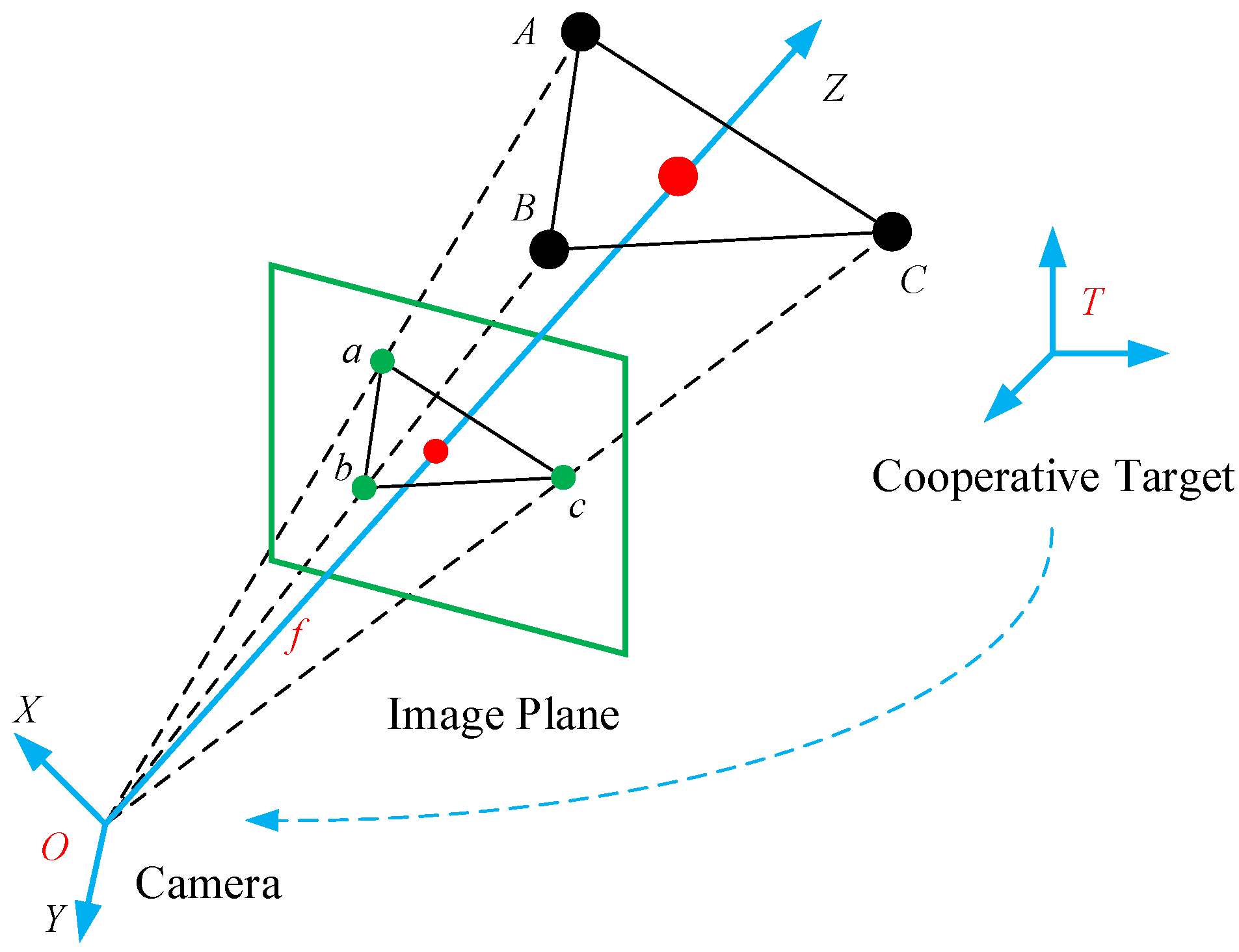
Figure 1 shows a calibrated camera and three known 3D points, A, B, and C. These points are projected onto the normalized image plane as a, b, and c [8]. One way to solve the P3P problem is to use simultaneous equations based on the law of cosines to first calculate the distances between three spatial points A, B, and C and the camera’s optical center. This is then followed by the determination of the locations of spatial points in the camera coordinate system according to the coordinates of projection points a, b, and c on the image plane. Without loss of generality, we choose points A and B for analysis.

Based on the work in [28], we assume that the coordinate of point A in the camera coordinate system is $(X_A,Y_A,Z_A)$. We further assume that the coordinate of point a in the image plane has an error $\delta a=\sqrt{\delta a_x^2+\delta a_y^2}$. In addition, we define the focal length of camera is as f. According to the imaging theorem, the errors of point A in the X and Y directions in the camera coordinate system are

$$\delta X_A=\frac{Z_A}{f}\times \delta a_x$$

(1)

$$\delta Y_A=\frac{Z_A}{f}\times \delta a_y$$

(2)

We introduce another space point, $B$, to analyze the error in the Z direction. When A and B are simultaneously moving along the Z direction, and we assume the error of line segment $\overline{ab}$ is $\delta ab$; then, according to [28], we obtain

$$\delta Z\propto \frac{Z_A^2}{AB\times f}\times \delta ab$$

(3)

Based on Equations (1)–(3), we can intuitively conclude that the error along the Z-axis is significantly higher than the errors along the other two axes. The position error along the Z-axis is directly proportional to the quadratic distance between the camera and the object. In contrast, the errors in the other two directions are directly proportional to the distance. Thus, when the measurement distance is significantly larger than the size of cooperative object, the translational error along the optical axis is higher than the errors along the other two axes.

We demonstrate the aforementioned difference in errors by means of an example: We consider a cooperative object of length $\overline{AB}=20 \mathrm{cm}$, the distance between the camera and object is 10 m, and the extraction error of the centroids of feature spots points is ${\delta }_a=0.1 \mathrm{pixels}$. The pixel size is 5.5 μm, the image size is 4096 × 3072 pixels, and the focal length of the camera is f = 600 mm. Using these parameters in Equations (1)–(3), we can find that the translational measurement accuracy along the optical axis of the camera is approximately 50 times lower than that along the other two axes. The actual experimental analysis is presented in Section 5.3.

3. Overview of the Proposed Camera and LRF Fusion System

This section is divided into three parts. The first part describes the composition of our system, which clarifies the subsequent description and derivation process and makes them easier to understand. The second part defines the relevant coordinate systems. The last part introduces the calculation process of the proposed 6-DOF pose measurement.

3.1. System Composition

As shown in Figure 2, the designed measurement system is mainly composed of four parts: an LRF, a monocular camera, a computer, and a cooperative target. As the researchers have already established relatively mature camera imaging and LRF measurement models, we will focus on the design of cooperative targets.

Our cooperative target consists of a laser corner cube prism and six red LEDs. Four LEDs are placed on the front panel of the target in a square configuration with a width of approximately 200 mm. The remaining two LEDs are placed on two slender rods whose length is approximately 200 mm. The laser corner cube prism is placed on the diagonal of the four LEDs. The relative positions of the six LEDs and corner cube prism are strictly calibrated using a three-coordinate measuring machine. The corner cube prism is used to reflect the laser, which ensures a laser distance measurement with ultra-high precision. In addition, as can be observed from the graph note in Figure 2, another advantage of the corner cube prism is that there is no stringent requirement on the incident point and incident angle of the laser beam, which helps to improve the measurement range and robustness.

3.2. Definition of the Coordinate Systems

The coordinate systems used in this article are defined as follows:

• Image pixel coordinate system (ICS, O): the rows and columns of the pixel plane are denoted by u and v, respectively.
• Camera optical coordinate system (CCS, O_C): the origin is the optical center of the camera. The optical axis direction of the camera is denoted by z_c, and x_c and y_c are parallel to u and v, respectively.
• Body coordinate system (BCS, O_B): the coordinate system is determined by the cooperative control points in the camera housing. The z_B, x_B and y_B axes point in the forward, right, and downward directions, respectively.
• LRF coordinate system (LCS, O_L): the z_L, x_L, and y_L axes point in the forward, right, and downward directions, whereas the laser line lies along the z_L-axis.
• Cooperative target coordinate system (TCS, O_T): the origin is defined by the center of the diagonal of the four LEDs on the coordinate target panel. The z_T, x_T, and y_T axes point in the backward, right, and downward directions, respectively.

The matrix $[R_{\alpha 2\beta },t_{\alpha 2\beta }]$ defines the conversion relations between the α-coordinate system and the β-coordinate system. $R_{\alpha 2\beta }$ is a 3 × 3 attitude rotation matrix, and $t_{\alpha 2\beta }$ is a 3 × 1 translation vector in α-coordinates. For example, $[R_{L2B},t_{L2B}]$ represents the relationship between the LCS and the BCS.

3.3. Calculation Process of Pose Measurement

First, we utilize the proposed parameters’ calibration process to calibrate the conversion relations $[R_{L2B},t_{L2B}]$ from the LCS to the BCS, and the conversion relations $[R_{C2B},t_{C2B}]$ from the CCS to the BCS, as shown in Figure 2.

Second, the monocular camera and the LRF are used to obtain image data and initial accurate depth data, respectively. We obtain the initial 6-DOF pose of cooperative targets based on the SRPnP [7] method, and then it can be transferred into the BCS using the calibrated parameters $[R_{C2B},t_{C2B}]$.

Third, we use the initial accurate depth data to correct the initial pose based on our proposed fusion strategy.

Last, we use an optimization model to optimize the 6-DOF pose and the fusion system parameters synchronously.

4. 6-DOF Pose Estimation

In this section, we will systematically present several key algorithms of our proposed method, including system calibration, data fusion, and system optimization.

4.1. Parameters Calibration

The proposed fusion system calibration includes two parts, as mentioned in Section 3.3. Most of the existing calibration methods [1,29,30] cannot be directly applied to the relationship between the BCS and the TCS, because the LRF uses invisible light. Thus, we introduce a laser tracker (Leica AT960) for the system parameter calibration. We assume that the accurate intrinsic matrix and radial distortion of the camera have been obtained using Zhang’s algorithm [31].

4.1.1. Extrinsic Parameters between LCS and BCS

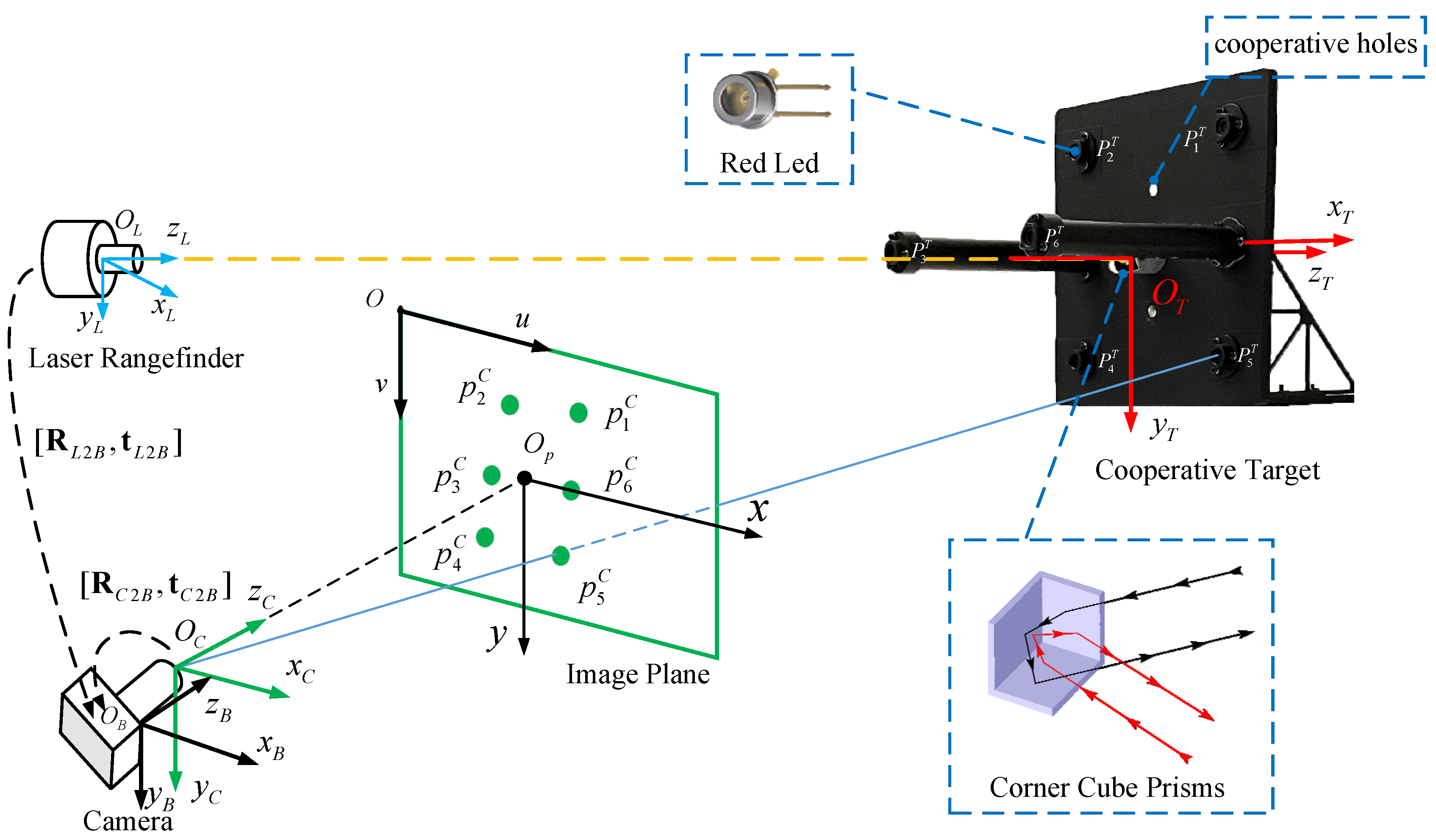
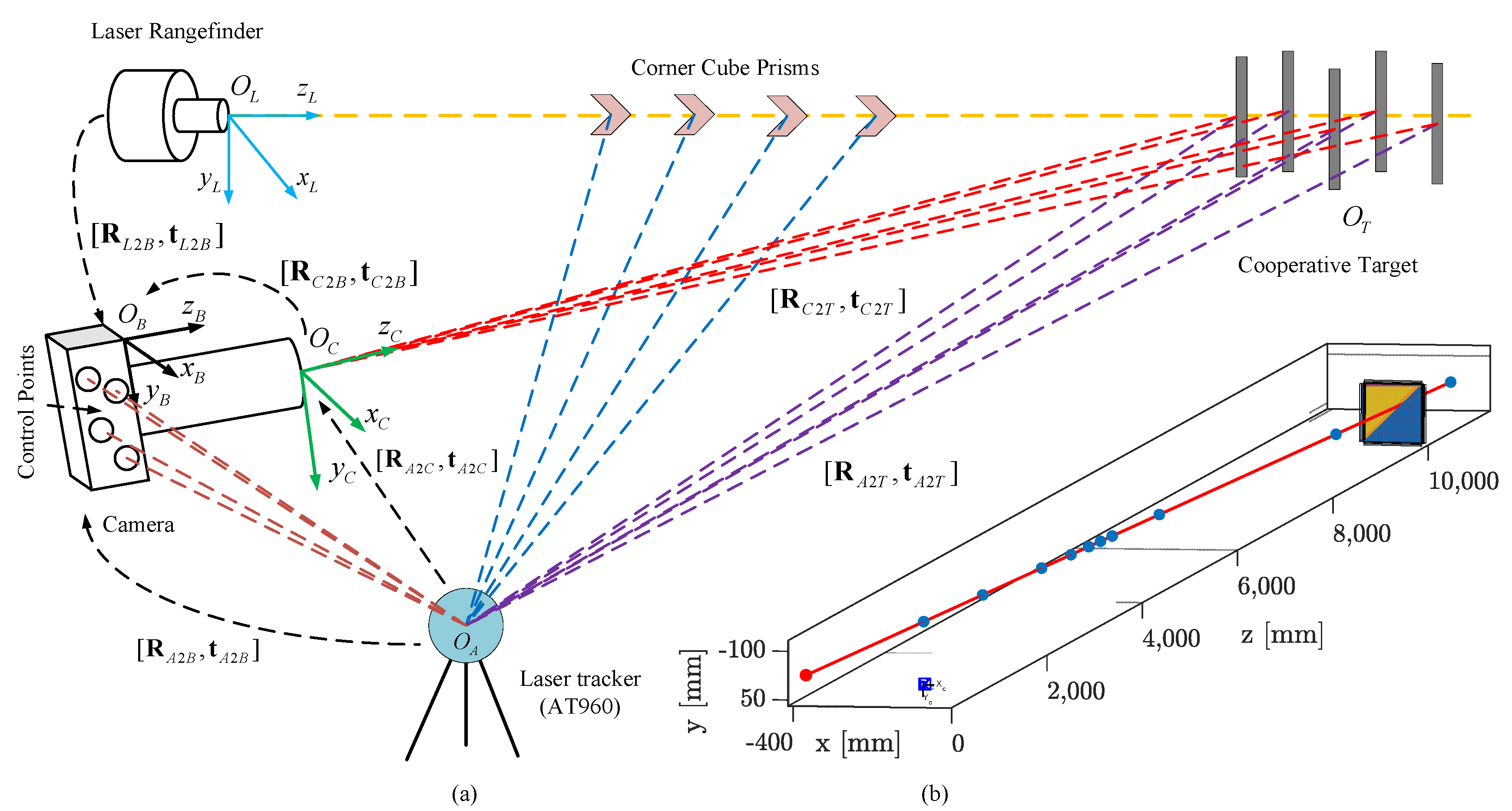
As illustrated in Figure 3a, the laser beam of the 1D LRF can be represented as a half-line with the origin $O_{LB}$ in the BCS, and we define the direction of the half-line by a unit norm vector $n_{LB}$. To reduce the number of parameters, we can use the origin $O_{LB}$ and unit norm vector $n_{LB}$ to represent the relationship between the LCS and the BCS; therefore, the extrinsic parameters of the laser tracker beam are as follows:

$$\begin{array}{l}{O}_{LB}={\left[x_L,y_L,z_L\right]}^T\\ n_{LB}={\left[n_{xL},n_{yL},n_{zL}\right]}^T\end{array}$$

(4)

Here, all vectors and points are expressed in the BCS.

We move the corner cube prism along the direction of the LRF laser beam several times. The position of the corner cube prism measured by AT460 and the measured values of the LRF are all recorded each time. As the laser beam is invisible, the feedback signal of the LRF can be used to ensure that the corner cube prism is along the laser beam. The direction $n_{LA}$ of the laser beam in the ASC can be calculated via straight-line fitting when we obtain all laser spots’ coordinates. Subsequently, the origin $O_{LA}$ in the ASC can be determined based on the ranging values measured by the LRF each time.

As Figure 3a shows, the four calibrated control points on the camera housing can be tracked using the Laser tracker to determine the conversion relations $[R_{A2B},t_{A2B}]$. Thus, the extrinsic parameters of the LCS to the BCS are

$$\begin{array}{l}{O}_{LB}=R_{A2B}·O_{LA}+t_{A2B}\\ n_{LB}=R_{A2B}·n_{LA}+t_{A2B}\end{array}$$

(5)

4.1.2. Extrinsic Parameters between CCS and BCS

As illustrated in Figure 3a, similar to the camera housing, there are also four control points on the cooperative target that can be used to determine the relationship $[R_{A2T},t_{A2T}]$ between the ACS and the TCS. The camera can determine the relationship $[R_{C2T},t_{C2T}]$ between the CCS and the TCS. Based on the relationship $[R_{A2B},t_{A2B}]$ relating the ASC to the BCS and the relationship $[R_{A2T},t_{A2T}]$ relating the ACS to the TCS, we can calculate the conversion relations $[R_{B2T},t_{B2T}]$ between the BCS and the TCS as the following expressions:

$$\begin{array}{l}{R}_{B2T}=R_{A2T}inv(R_{A2B})\\ t_{B2T}=R_{A2B}(t_{A2T}-t_{A2B})\end{array}$$

(6)

where $inv{(}^{})$ represents matrix inversion.

Now, using the relationship $[R_{C2T},t_{C2T}]$ between the CCS and the TCS, which are obtained by the camera and the relationship $[R_{B2T},t_{B2T}]$ between the BCS and the TCS, we can calculate the relationship $[R_{C2B},t_{C2B}]$ between the CCS and the BCS as

$$\begin{array}{l}{R}_{C2B}=inv(R_{B2T})R_{C2T}\\ t_{C2B}=t_{C2B}+inv(R_{C2T})R_{B2T}{t}_{B2T}\end{array}$$

(7)

Based on Equations (6) and (7), an initial value of the extrinsic parameters $[R_{C2B},t_{C2B}]$ between the CCS and the BCS can be obtained experimentally. Next, we will use more data to iteratively optimize the initial parameter values.

We define the pose relationship matrix between the CCS and the TCS derived from $[R_{C2B},t_{C2B}]$ and $[R_{B2T},t_{B2T}]$ as $[R_{C2T}^{\prime },t_{C2T}^{\prime }]$. According to the coordinate system conversion relations, $[R_{C2T}^{\prime },t_{C2T}^{\prime }]$ can be calculated by

$$\{\begin{array}{l}{R}_{C2T}^{\prime }=R_{B2T}{R}_{C2B}\\ t_{C2T}^{\prime }=t_{C2B}+inv(R_{C2B})t_{B2T}\end{array}$$

(8)

According to the 6-DOF pose given in Equation (8), we can obtain six re-projection imaging points $P_i^T(i=1,2,\dots ,6)$ on the image plane with the help of the imaging theorem and the calibrated parameters. Then, we can calculate the Euclidean distance between each re-projection imaging point and its corresponding actual imaging point $p_i^C(i=1,2,\dots ,6)$, namely the reprojection error. A total of $n$ measurements are acquired by changing the azimuth and angle of the cooperative target and recording the results after each change. We utilize an iterative optimization scheme for all measurements by minimizing the reprojection errors of six LED points on the cooperative target. The following objective function is optimized:

$$\underset{K,R_{C2B},t_{C2B},\left\{X_{led},Y_{led},Z_{led}\right\}}{minimize}={\displaystyle \sum _{j=1}^n\left({\displaystyle \sum _{i=1}^6\left|p_{i,j}^C-pro(P_{i,j}^T)\right|}\right)}$$

(9)

where $K$ represents the intrinsic matrix of the camera, $R_{C2B}$ and $t_{C2B}$ are the extrinsic parameters relating the CCS to the BCS, $\left\{X_{led},Y_{led},Z_{led}\right\}$ represent the coordinates of six LED points in the TCS, and $pro(P_{i,j}^T)$ is the projection functions of six LED points based on the pose relationship between the CCS and the TCS $[R_{C2T}^{\prime },t_{C2T}^{\prime }]$.

The rotation matrix $R_{C2B}$ is parametrized using the Cayley–Gibbs–Rodriguez (CGR) theorem [32]. It can be expressed as a function of the CGR parameters $s=\left[\begin{array}{ccc}{s}_1& s_2& s_3\end{array}\right]$, as follows:

$$R_{C2B}=\frac{1}{1+s_1^2+s_2^2+s_3^2}·\left[\begin{array}{ccc}1+s_1^2-s_2^2-s_3^2& 2s_1{s}_2-2s_3& 2s_1{s}_3+2s_2\\ 2s_1{s}_2+2s_3& 1-s_1^2+s_2^2-s_3^2& 2s_2{s}_3-2s_1\\ 2s_1{s}_3-2s_2& 2s_2{s}_3+2s_1& 1-s_1^2-s_2^2+s_3^2\end{array}\right]$$

(10)

Subsequently, the problem will be transformed into an unconstrained optimization problem. By solving Equation (9) based on the Levenberg–Marquardt optimization method [33,34], we can obtain accurate calibration parameters of the intrinsic matrix of the camera $K$, extrinsic parameters relating the CCS to the BCS $[R_{C2B},t_{C2B}]$, and the coordinates of six LED points in the TCS $\left\{X_{led},Y_{led},Z_{led}\right\}$; Figure 3b shows the results of applying the proposed calibration procedure to our setup comprising a camera and an LRF.

In this subsection, we obtained the conversion relations that transfer the initial 6-DOF pose measured by the camera to the BCS, as well as calculated the origin of the LRF and the direction of the laser line in the BCS. In the following subsection, we will design an algorithm to obtain the ultra-high precision 6-DOF pose of the cooperative target.

4.2. Pose Acquisition and Fusion

The accurate depth $D_a$ measured by the LRF can be directly used by the fusion algorithm. We use a series of image processing algorithms to detect the centroid of the imaging points $p_i^C(i=1,2,\dots ,6)$ of six LEDs. The different steps of this algorithm include image filtering, circle detection, and centroid acquisition [35]. The coordinates of six LEDs under the cooperative target coordinate system (TCS) are denoted by $P_i^T(i=1,2,\dots ,6)$.

As Figure 3a shows, we have six cooperative points in the TCS and their corresponding image coordinates in the ICS. The calculation of the relative 6-DOF pose between the camera and the cooperative target belongs to the PnP problem mentioned in Section 1.

The corresponding relationship between $P_i^T$ and $p_i^C$ is given by the following expression:

$$s{P}_i^T=K(R_C{p}_i^T+t_C)$$

(11)

where $K$ is the intrinsic matrix of the camera, and $s$ is a depth scale factor. The rotation matrix and the translation vector relating the CCS to the TCS measured by the camera based on the SRPnP method are denoted by $R_C$ and $t_C$, respectively. Subsequently, we transfer them to the BCS using the following expressions:

$$R_B=\left[\begin{array}{ccc}{R}_{11}& R_{12}& R_{13}\\ R_{21}& R_{22}& R_{23}\\ R_{31}& R_{32}& R_{33}\end{array}\right]=R_{C}inv(R_{C2B})$$

(12)

$$t_B=\left[\begin{array}{c}{t}_x\\ t_y\\ t_z\end{array}\right]=R_{C2B}(t_C-t_{C2B})$$

(13)

where R_B meets the orthogonal constraint of the rotation matrix and has three degrees of freedom. Thus, we obtain the initial 6-DOF pose and accurate depth value between the BCS and the TCS. Our goal is to use the depth value $D_a$ to correct the $t_z$ component of the 6-DOF pose.

However, as illustrated in Figure 4, the laser beam has an inevitable width. In other words, the laser spot is diffuse. This means that the laser corner cube prism does not necessarily lie on the straight line $L_{LT}$ defined by the center of the laser beam and, therefore, the depth value of LRF cannot be directly used. However, we are certain that the laser corner cube prism is on the laser spot.

Without loss of generality, we assume that the laser spot is a plane that passes through the point $P=\left\{x_r, y_r, z_r\right\}$, which is located in the center line of laser beam $L_{LT}$. The line $L_{LT}$ can be represented by an origin $O_{LB}={\left[x_L,y_L,z_L\right]}^T$ and a unit norm vector $n_{LB}={\left[n_{xL},n_{yL},n_{zL}\right]}^T$. We can obtain $O_{LB}$ and $n_{LB}$ by calibrating the transformation parameters of the BCS and the LCS. Thus, the equation of line $L_{LT}$ can be expressed as

$$\frac{x-x_L}{n_{xL}}=\frac{y-y_L}{n_{yL}}=\frac{z-z_L}{n_{zL}}$$

(14)

We can easily observe that the direction vector of the plane is parallel to the direction vector $n_{LB}={\left[n_{xL},n_{yL},n_{zL}\right]}^T$ of line $L_{LT}$. In addition, the distance from the origin of the LCS to the plane is the actual measurement value of the LRF. According to the above conditions, the equation of the plane can be solved by the following simultaneous equations:

$$\{\begin{array}{l}{n}_{xL}(x-x_r)+n_{yL}(y-y_r)+n_{zL}(z-z_r)=0\\ \frac{x_r-x_L}{n_{xL}}=\frac{y_r-y_L}{n_{yL}}=\frac{z_r-z_L}{n_{zL}}\\ {(x_r-x_L)}^2+{(y_r-y_L)}^2+{(z_r-z_L)}^2=D_a^2\end{array}$$

(15)

We know that the 6-DOF pose of the cooperative target consists of the rotational DOF $R_B$ as well as the translational DOF $t_B$. They can define a line segment $L_{BT}$ whose starting and ending coordinates are the origins of the BCS and TCS, respectively. As mentioned earlier, the other values in the 6-DOF pose are relatively accurate, except for the translational DOF along the $z_B$-axis of the BCS.

We utilize the vector $t_b={\left[\begin{array}{ccc}{t}_x& t_y& t_z\end{array}\right]}^T$ to denote the initial translational DOF of the cooperative target. The measured initial origin and the precise origin of the cooperative target are represented as $O_T^i={\left[t_x,t_y,t_z\right]}^T$ and $O_T^r={\left[x_T,y_T,z_T\right]}^T$, respectively. Thus, the translational DOF measurement error along the $z_B$-axis is as follows:

$$\Delta z=t_z-z_T$$

(16)

According to the previous discussion, we know that

$$\{\begin{array}{l}{x}_T\approx t_x\\ y_T\approx t_y\\ t_z\gg (t_x\&t_y)\gg (\Delta z=t_z-z_T)\end{array}$$

(17)

Therefore, as shown in Figure 4, within the allowable error range, we can assume that the precise origin of the cooperative target $O_T^r$(red point) lies on the line defined by the initial origin of the cooperative target $O_T^i$ (black point) and the origin of the BCS. This signifies that the starting coordinate and the direction of the line segment $L_{\mathrm{BT}}$ are accurate. On the contrary, the endpoint coordinate has a large error in the $z_B$-axis. In other words, the precise origin of the cooperative target $O_T^r$ has an uncertainty of $d_z$.

Let us represent the slopes of the line $L_{BT}$ by a unit vector $\overrightarrow{L_{BT}}=[l,m,n]$. Thus, the equation of the line $L_{BT}$ is

$$\frac{x-0}{l}=\frac{y-0}{m}=\frac{z-0}{n}$$

(18)

Subsequently, we obtain the straight-line parameters $\left\{l,m,n\right\}$ by substituting $O_t^i={\left[t_x,t_y,t_z\right]}^T$ into Equation (18).

Now, we know that the precise origin of the cooperative target $O_T^r$ is not only on the straight-line $L_{BT}$, but also on the plane of the laser spot $P$. Therefore, as shown in Figure 4, our fusion strategy becomes a mathematical problem to find the intersection point (red point) of a spatial plane (blue curve) and a spatial line (green line) in the BCS, expressed as follows:

$$\{\begin{array}{l}{n}_{xL}(x-x_r)+n_{yL}(y-y_r)+n_{zL}(z-z_r)=0\\ \frac{x_r-x_L}{n_{xL}}=\frac{y_r-y_L}{n_{yL}}=\frac{z_r-z_L}{n_{zL}}\\ {(x_r-x_L)}^2+{(y_r-y_L)}^2+{(z_r-z_L)}^2=D_a^2\\ \frac{x}{l}=\frac{y}{m}=\frac{z}{n}\end{array}$$

(19)

By solving Equation (19), we can obtain the precise coordinates $O_T^r={\left[x_t,y_t,z_t\right]}^T$ of the origin of the cooperative target. So far, we have corrected the initial 6-DOF pose using the accurate depth value of LRF.

4.3. Bundle Adjustment

We utilize an optimized scheme for each correction result to further improve the accuracy. This scheme minimizes the combination of the error of the initial depth and the corrected depth as well as the reprojection errors of the six LED points of the cooperative target as follows:

$$\underset{R_B,O_T^r}{minimize}={\displaystyle \sum _{i=1}^6{\Vert p_i^C-pro(P_i^T)\Vert }_2}+\lambda {\Vert z_t-t_z\Vert }_2$$

(20)

where $p_i^C$ represents the coordinates of the imaging points of six LEDs in the image coordinate system, and $pro(P_i^T)$ represents the projection functions of six LED points. A weight parameter is denoted by $\lambda$, which should be adjusted to normalize the variance of camera and LRF residue distributions. Generally, its value is fixed as $\lambda =5$.

Minimizing Equation (20) as a nonlinear optimization problem based on the Levenberg–Marquardt method, we will obtain an accurate 6-DOF pose of the cooperative target in the BCS.

5. Experimental Results

A series of experiments are performed in this section to validate the sensor fusion method proposed in this paper and evaluate the performance of the 6-DOF pose measurement system. First, we introduce the experimental setup in Section 5.1. Then, in Section 5.2, we describe the fusion system calibration experiment. Last, in Section 5.3, simulation experiments are described that are used to evaluate the effects of image noise and the size of cooperative target on the measurement accuracy. In addition, details of actual experiments carried out to evaluate the 6-DOF pose measurement accuracy of our fusion system are provided.

Table 2. Prototype parameters of the proposed multi-sensor fusion-based 6-DOF pose measurement system.

Parameter	Value
Measuring range	10 ± 0.2 m (adjustable)
Absolute accuracy	20 μm (15″)
Operating temperature	−20 °C–30 °C;
Weight	3.5 kg
FPS	4 Hz

shows the parameters of the fusion sensor that was built according to the proposed fusion method. We can observe that it has an impressive 6-DOF pose measurement precision.

5.1. Experimental Setup

Figure 5 shows the layout of our experiment and our proposed fusion sensor. The cooperative target and the fusion system are placed approximately ten meters apart, with the Leica Absolute Tracker (AT960) in the middle. The 6-DOF pose change of the cooperative target is controlled using the motion platform. The AT960 can obtain the actual 6-DOF position using the control points on the cooperative target and the camera housing. As the positional accuracy of AT960 can reach 15 μm, its measurements are defined as true values.

Table 3. System parameters of camera and LRF.

Sensor	Parameter	Value
Camera	Resolution	4096(H) × 3072(V)
	Frame rate	10 FPS
	Pixel size	5.5 µm × 5.5 µm
	Focus	510 mm
	Weight	450 g
LRF	Wavelength	1558 nm
	Range	1~20 m
	Accuracy	2 × 10−3 mm

shows the relevant parameters of the camera and LRF of our proposed system.

5.2. System Calibration Experiment

In this subsection, we describe the experiments conducted on the calibration method described in Section 4.1. First, the intrinsic parameters of the camera were calibrated using Zhang’s algorithm [31].

Table 4. Intrinsic parameters of the camera.

Parameter	f	cx	cy
Value	508.877	2049.653	1542.325
Parameter	Radial distortion	Eccentric distortion
Value	$\begin{array}{l}k1=-1.8388\times {10}^{-6}\hfill \\ k2=5.7822\times {10}^{-9}\hfill \\ k3=-9.9989\times {10}^{-12}\hfill \end{array}$	$\begin{array}{l}p1=-3.5379\times {10}^{-6}\hfill \\ p2=1.13724\times {10}^{-6}\hfill \end{array}$

shows the intrinsic parameters and radial distortion of the camera.

Next, based on the laser beam calibration method mentioned in Section 4.1.1, we moved the corner cube prism along the direction of the LRF’s laser beam. Subsequently, the AT460 and LRF were used to record the 3D coordinates and depth values of 10 points, and then these coordinates are transferred to the BCS. Then, we used those 3D coordinates to fit a line based on the least-squares method. Subsequently, we calculated the origin of the LRF by combining it with the depth values of each point.

Table 5. Calibrated extrinsic parameters from LRF (LCS) to BCS.

Parameter	${\mathit{x}}_{\mathit{L}}$	${\mathit{y}}_{\mathit{L}}$	${\mathit{z}}_{\mathit{L}}$	${\mathit{n}}_{\mathit{x}\mathit{L}}$	${\mathit{n}}_{\mathit{y}\mathit{L}}$	${\mathit{n}}_{\mathit{z}\mathit{L}}$
Value (mm)	−416.2655	84.1989	360.815	0.0511	−0.0016	0.9987

shows the origin and direction of the LRF semi-line.

Last, during the calibration of the extrinsic parameters relating the CCS to the BCS, we changed the azimuth and angle of the cooperative target to obtain 120 poses. After moving the cooperative target each time, the monocular camera system captured the images, calculated the relative pose, and saved the data. Simultaneously, the laser tracker measured and saved the 6-DOF pose relating the BCS to the TCS. As mentioned earlier, we can consider that the measurements of the AT460 are the true values of the relative 6-DOF pose between the BCS and the TCS.

We could obtain an initial value of the extrinsic parameters between the CCS and the BCS using a set of data based on Equation (8). Then, we inputted other data into Equation (9) and solved the nonlinear optimization problem based on the Levenberg–Marquardt iterative optimization method. As shown in Equation (9), the intrinsic parameters of the camera, the extrinsic parameters between the CCS and the BCS, and the coordinates of the LED points in the TCS were all optimized.

Table 6. Calibrated extrinsic parameters from the CCS to the BCS.

Parameter	${\mathit{R}}_{\mathit{C}2\mathit{B}}^{\mathit{x}}$	${\mathit{R}}_{\mathit{C}2\mathit{B}}^{\mathit{y}}$	${\mathit{R}}_{\mathit{C}2\mathit{B}}^{\mathit{z}}$	${\mathit{T}}_{\mathit{C}2\mathit{B}}^{\mathit{x}}$	${\mathit{T}}_{\mathit{C}2\mathit{B}}^{\mathit{y}}$	${\mathit{T}}_{\mathit{C}2\mathit{B}}^{\mathit{z}}$
Value (mm)	0.1549	−0.0334	0.0481	48.6467	−134.0844	−353.1991

shows the calibration results of the extrinsic parameters between the CCS and the BCS.

5.3. Simulation Experiments

It is known that the centroid extraction accuracy of the feature points in the cooperative target and its size strongly influence the pose measurement accuracy. Therefore, we verified the influence of these two factors on our proposed 6-ODF pose measurement method through simulation experiments.

We used MATLAB R2019a software on Windows 10 to carry out the simulation experiments. To represent a realistic measuring environment, we fixed the relevant simulation system parameters equal to the calibration values of our system.

Table 7. Real pose between the TCS and the BCS in simulations.

Parameter	${\mathit{R}}_{\mathit{x}}$	${\mathit{R}}_{\mathit{y}}$	${\mathit{R}}_{\mathit{z}}$	${\mathit{T}}_{\mathit{x}}$	${\mathit{T}}_{\mathit{y}}$	${\mathit{T}}_{\mathit{z}}$
Value (mm)	0.2	2.1	0.5	−140	−32	10,000

shows the true pose between the TCS and the BCS used in the simulation experiments.

First, we validated the influence of centroid extraction error on 6-ODF pose measurement accuracy. Throughout the experiment, we compared the calculated 6-DOF pose values with the real pose values. The difference between both values is the measurement error of our proposed multi-sensor fusion-based 6-DOF pose measurement method.

We added ${\omega }_{noise}\sim Gauss(0,{\Sigma }_{noise})$ Gaussian noise to the centroid of the extracted LED image points, where ${\Sigma }_{noise}$ is the standard deviation of the Gaussian distribution. We increased ${\Sigma }_{noise}$ gradually from 0.01 to 0.36 pixels. For each noise level, we performed 100 independent experiments. The errors between the measured value and true poses are shown in Figure 6. The red horizontal lines represent the median, and the borders of the boxes represent the first and third quartiles, respectively. The measurement results marked with a red “+” symbol represent high noise in the simulation. It can be observed from Figure 6 that the measurement errors in all directions increase with the increase in noise level. When the centroid extraction noise is 0.15 pixels, the translational and rotational DOF errors in all directions are approximately 0.02 mm and 15″, respectively.

We also analyzed the influence of the size of the cooperative target on the pose measurement accuracy. The size was changed gradually from 50 mm to 150 mm. We performed 100 independent experiments for each size of the cooperative target, and the results are shown in Figure 7. We can see that, in our proposed multi-sensor fusion-based 6-DOF pose measurement method, the changing size of the cooperative target slightly impacts the translation vector, but significantly impacts the attitude rotation angle.

5.4. Real Experiments

We also evaluated the performance of the proposed fusion system by conducting actual experiments, in which multiple static measurements were taken at the same pose, and measurements were tracked at various poses.

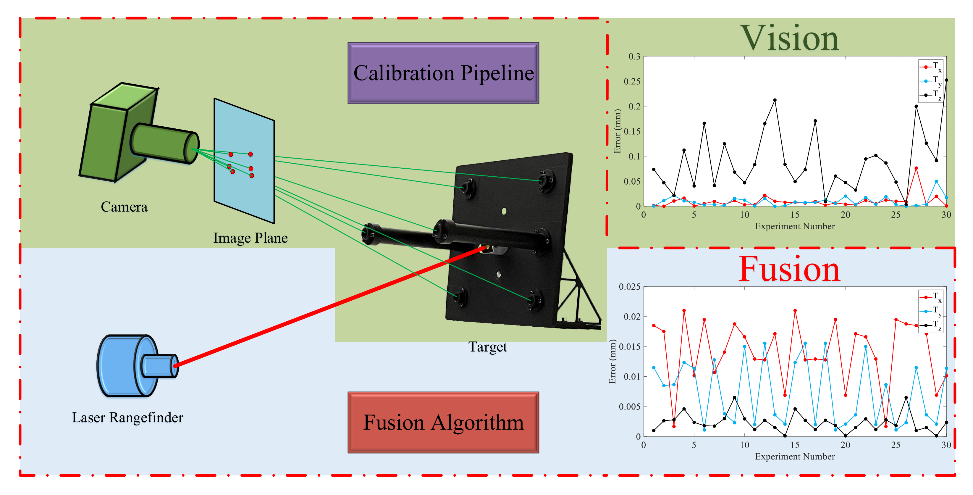
First, the cooperative target was kept stationary, and we performed 30 6-DOF pose measurements using the proposed fusion system and laser tracker (AT460) simultaneously. Then, we calculated the initial and final 6-DOF pose. The initial 6-DOF pose values were measured directly by the monocular camera, and the corresponding final 6-DOF pose values were obtained using our proposed fusion method. As mentioned earlier, we assume that the results measured by the laser tracker are the true values. We subtracted those true values from both the initial and final 6-DOF pose values. The corresponding differences are the measurement errors of the initial and final poses.

As shown in Figure 8, compared with the initial pose, we can observe that the final pose is improved in both translational and rotational DOF. In particular, the accuracy of translational DOF in the z-axis shows a 50-fold increase corresponding to the calculations in Section 2. The maximum errors of $T_x$, $T_y$, $T_z$, $R_x$, $R_y$, and $R_z$ are 0.0130 mm, 0.0114 mm, 0.0016 mm, 6.634″, 5.452″, and 11.113″, respectively. The reduction in the translational DOF error in the z-axis is mainly due to our fusion strategy, while the reduction in other degrees of freedom error is mainly due to the contribution made by our bundle adjustment optimization in Section 4.3.

We also conducted tracking measurement experiments at different poses to check the accuracy of our proposed fusion system. We place the cooperative target approximately 10 m away from our fusion system and acquired 30 frames of measurement data by changing the azimuth and angle of the cooperative target. The final 6-DOF pose obtained by the proposed method over 30 measurements are calculated and optimized based on the methods proposed in Section 4.

We use ($R_x$, $R_y$, $R_y$, $T_x$, $T_y$, and $T_z$) to represent the 6-DOF pose of the cooperative target measured by the proposed fusion system, and ($R_x^{\prime }$, $R_y^{\prime }$, $R_y^{\prime }$, $T_x^{\prime }$, $T_y^{\prime }$, and $T_z^{\prime }$) to represent the true 6-DOF pose measured by the laser tracker AT460. Figure 9 shows the measured value, true value, and error over 30 tracking measurements drawn in the form of line graphs. The blue curve represents the value measured by the proposed system, the black curve represents the true value measured by the laser tracker, and the red curve is the absolute value of the difference between these two values, namely the measurement error of our system.

6. Conclusions

We proposed a novel approach to overcome the shortcomings of existing monocular camera 6-DOF pose estimation methods for cooperative targets. This approach was based on the fusion of a monocular camera and an LRF. The proposed approach first obtained the initial 6-DOF pose and accurate depth value. We used the initial 6-DOF pose to obtain a space line, and the LRF spot was modeled as a space circle surface. The exact position of the cooperative target was then obtained by finding the intersection of the space line and the space circle surface. Finally, we further improved the measurement accuracy and system parameters by minimizing the error of initial and actual depth values and the reprojection errors of the six LED points of the cooperative target. The main contribution of the proposed method, compared with other camera-LRF fusion methods, was the elimination of error produced by the laser spot size. In addition, we proposed a novel parameter calibration pipeline for the camera and LRF fusion system, which could calibrate the LRF that was not visible in the camera. Simulations and experimental results showed that our fusion method significantly improved the accuracy of monocular vision 6-DOF pose measurement. The fusion 6-DOF pose estimation sensor that we built achieved an impressive precision compared to other remote 6-DOF pose measurement methods. The results with the built sensor were close to the expensive laser tracker measurement results.