
Performance of Single-Epoch EWL/WL/NL Ambiguity-Fixed Precise Point Positioning with Regional Atmosphere Modelling


1
School of Instrument Science and Engineering, Southeast University, Nanjing 210096, China
2
Key Laboratory of Micro-Inertial Instrument and Advanced Navigation Technology, Southeast University, Nanjing 210096, China
3
School of Transportation, Southeast University, Nanjing 210096, China
4
The Sino-UK Geospatial Engineering Centre, Nottingham NG8 1NA, UK
*
Author to whom correspondence should be addressed.
Remote Sens. 2021, 13(18), 3758; https://0-doi-org.brum.beds.ac.uk/10.3390/rs13183758
Submission received: 20 August 2021
/
Revised: 16 September 2021
/
Accepted: 17 September 2021
/
Published: 19 September 2021
(This article belongs to the Special Issue Integrated Applications of Real-Time GNSS Precise Positioning Services)
Abstract
:Precise point positioning (PPP) with ambiguity resolution (AR) can improve positioning accuracy and reliability. The narrow-lane (NL) AR solution can reach centimeter-level accuracy but there is a certain initialization time. In contrast, extra-wide-lane (EWL) or wide-lane (WL) ambiguity can be fixed instantaneously. However, due to the limited correction accuracy of the empirical atmospheric model, the positioning accuracy is only a few decimeters. In order to further improve the real-time performance of PPP while ensuring accuracy, we developed a multi-system multi-frequency uncombined PPP single-epoch EWL/WL/NL AR method with regional atmosphere modelling. In the proposed method, the precise atmosphere, including zenith wet-troposphere delay (ZWD) and the slant ionosphere, is extracted through multi-frequency stepwise AR, which then is both interpolated and broadcast to users. By adding regional atmosphere constraints, users can achieve single-epoch PPP AR with centimeter-level accuracy. To verify the algorithm, four sets of reference networks with different inter-station distances are used for experiments. With atmosphere constraints, the accuracy of the single-epoch WL solution can be improved from the decimeter level to a few centimeters, with an improvement of more than 90%, and the epoch fix rate can also be improved to varying degrees, especially for the dual-frequency case. Due to the enlarged noise of the EWL combination, its accuracy is at the decimeter level, while the accuracy of the WL/NL solution can reach several centimeters. However, reliable NL ambiguity-fixing tightly relies on atmosphere constraints with sufficiently high accuracy. When the modelling of the atmosphere correction is not accurate enough, the NL AR performance is degraded, although this situation can be improved to a certain extent through the multi-GNSS combination. In contrast, in this case, the WL ambiguity can be successfully fixed and can support the precise positioning with an accuracy of several centimeters.
1. Introduction
As a wide-area high-precision positioning technology, precise point positioning (PPP) has been widely used in deformation monitoring, precise timing, and other fields [1,2,3]. However, it usually requires a long convergence time to achieve centimeter-level accuracy and leads to a poor real-time performance. PPP ambiguity resolution (AR) can shorten the initialization time to a certain extent. However, due to the strong correlation between various parameters, reliable AR also requires tens of minutes [4,5]. These problems have also become the bottleneck of the development of PPP technology. With the modernization of the Global Positioning System (GPS) and Global Navigation Satellite System (GLONASS), and the continuous improvement of Galileo, the BeiDou Navigation Satellite System (BDS) and the Quasi-Zenith Satellite System (QZSS), many satellites can broadcast navigation signals at three or more frequencies. Additionally, the Global Navigation Satellite System (GNSS) has officially entered an era of multi-system co-existence. The multi-system and multi-frequency GNSS signals provide new opportunities for the improvement of positioning performance.
During the research of GPS/BDS/Galileo/GLONASS combined PPP, Li et al. [6] emphasized that multi-system fusion can significantly improve the positioning performance of PPP in harsh environments. Even in the case of the 40° cut-off elevation angle, it can still achieve relatively stable positioning results. In addition, the convergence time can be generally shortened from nearly 20 min to about 10 min. Guo et al. [7] proposed three triple-frequency PPP models based on real-tracked BDS observations and the results showed that different models show high consistency. The additional frequency has little effect on static PPP but in case of poor observation conditions, the performance of kinematic PPP can be slightly improved. Taking GPS as an example, Pan et al. [8] further demonstrated the mathematical equivalence of the different triple-frequency PPP models in the convergence stage and the accuracy difference between the results of different models was usually no more than 6 mm. Aimed at the unified multi-frequency ionosphere-free (IF) model, Elsobeiey [9] and Viet Duong et al. [10] emphasized that the convergence of PPP can be accelerated by selecting optimal linear combinations. In addition, some scholars have also compared the positioning performance of multi-frequency PPP and traditional dual-frequency PPP, and the results show that the positioning accuracy and convergence time of the multi-frequency combination are always better than that in the dual-frequency case [11,12].
Compared with the dual-frequency case, the major advantage of multi-frequency observations is that a variety of combinations with excellent characteristics, such as long wavelength and weak ionosphere, can be formed through linear transformation, thereby providing new opportunities for rapid PPP AR. Based on simulated triple-frequency GPS signals, Geng and Bock [13] proposed a triple-frequency PPP AR algorithm in which ambiguities of extra-wide-lane (EWL), wide-lane (WL), and narrow-lane (NL) are fixed sequentially; using constraints of ambiguity-fixed ionosphere-free (AFIF) observations instead of the original pseudorange, the correct fixing rate of NL ambiguity is increased to 99% within 65 s, in contrast to only 64% within 150 s in the dual-frequency case. Later, Li et al. [14,15] introduced a similar idea into BDS/Galileo multi-frequency PPP, and analyzed the AR performance of triple-frequency, quad-frequency, and five-frequency PPP with different combination coefficients. They came to the conclusion that regardless of the time to first fix (TTFF) or positioning accuracy, the results of the multi-frequency was always better than that of the dual-frequency. In addition to the above AFIF-based multi-frequency AR strategy, as the uncombined PPP model has gradually become the standard for multi-frequency data processing, many scholars have studied the AR method based on multi-frequency uncombined PPP. Gu et al. [16] and Li et al. [17] extracted the EWL/WL/NL fractional cycle bias (FCB) of BDS through integer transformation and compared the AR performance of both the triple-frequency and dual-frequency case; the results showed that the accuracy of triple-frequency AR was higher in the initialization phase. In addition, Liu et al. [18] also used the least-squares ambiguity decorrelation adjustment (LAMBDA) algorithm to determine the optimal coefficients in the linear transformation process. Geng et al. [19] further evaluated the AR performance of GPS/BDS/Galileo/QZSS based on triple-frequency uncombined PPP and the results showed that under the constraints of EWL/WL AR, the TTFF of NL ambiguity could be effectively reduced. In addition to assisting NL ambiguity-fixing, another advantage of multi-frequency AR is that the EWL/WL combination with long wavelengths is not sensitive to residual errors, thus it is expected to achieve single-epoch-fixing [20]. Based on real-tracked vehicle-borne data, Geng et al. [21,22] found that the single-epoch wide-lane ambiguity resolution (WAR) could reach an accuracy of the decimeter level. Guo and Xin [23] further emphasized that utilizing the advantage of low noise amplification of the Galileo E1/E5a/E6 combination, the positioning accuracy could theoretically be further improved to about 10 cm.
In general, multi-system and multi-frequency can greatly shorten the initialization time of PPP. However, due to the short wavelength of NL ambiguity, it is still difficult to fix instantaneously. In contrast, the EWL/WL ambiguity can generally be fixed using a single epoch of data; however, due to lack of high-precision atmosphere correction, the conventional single-epoch WAR can only reach an accuracy of the decimeter level. Achieving real-time centimeter-level positioning, similar to network real-time kinematic (NRTK) positioning, has always been the pursuit of PPP researchers. Based on the dual-frequency IF model, Li et al. [24,25] studied the precise atmosphere augmented PPP and achieved instantaneous fixing of the NL ambiguity by directly correcting the atmosphere error of observations.
The aforementioned scholars’ research has initially verified the feasibility of single-epoch PPP AR. With the development of multi-GNSS and multi-frequency, the single-epoch PPP AR with multi-scale accuracy still lacks targeted research. For this reason, this paper is mainly oriented to multi-system and multi-frequency signals based on a unified multi-frequency uncombined PPP model, and the performance of single-epoch EWL/WL/NL ambiguity-fixed solutions enhanced by regional atmosphere are analyzed in detail. In addition, this positioning mode can also meet the diversified requirements for the positioning accuracy of different industries.
The article is structured as follows. In Section 2, the multi-frequency uncombined PPP model, multi-frequency FCB estimation method, stepwise AR strategy, and regional atmosphere modelling method are discussed. In Section 3, the data process strategy is briefly described and the results of the multi-frequency FCB, regional atmosphere modelling, and single-epoch AR performance are analyzed successively. In Section 4, the characteristics of the single-epoch EWL/WL/NL ambiguity-fixed solution is discussed. Some conclusions are given in Section 5.
2. Methods
2.1. Multi-Frequency Uncombined PPP Model
The undifferenced pseudorange and carrier phase observation on the raw frequency can be expressed as [6,14,22]
where indices refer to the satellite, receiver, and carrier frequency band, respectively; and are the pseudorange and carrier phase observations in the unit of length; is the geometric distance between the receiver and satellite; and are the zenith wet-troposphere delay (ZWD) and the corresponding mapping function; is the speed of light in vacuum; and are the receiver and satellite clock bias, respectively; is the slant ionosphere delay at the first frequency; is the ionosphere factor; is the integer ambiguity with wavelength ; and are the receiver and satellite code bias in the unit of length; and are the receiver and satellite phase bias in the unit of cycle; and lastly and denote the measurement noise in the pseudorange and phase observations. One thing to note is that the errors not listed in the formula, such as the phase center offsets (PCO), variations (PCV), phase windup, etc., need to be accurately corrected using existing models [26,27].
Due to the correlation between various estimated parameters, parameter realignment is usually required in PPP processing. Based on the assumption that the satellite-related hardware bias is stable over time, it is usually lumped together with ambiguity parameters and is estimated as float constants. However, with the development of multi-frequency GNSS, many scholars have found that this assumption is not strict during the precise clock estimation process, especially for GPS Block IIF and BDS-2. The additional third frequency presents an obvious phase anomaly phenomenon, which exhibits periodicity related to its orbital period [28,29,30]. This means that the traditional precise clock product associated with the dual-frequency IF combination cannot be directly applicable to multi-frequency PPP data processing. To compensate for the impact, the concept of the inter-frequency clock bias (IFCB) is introduced and the phase bias is also rewritten into the following form [31]:
where and denote the time-invariant and time-varying parts of satellite phase bias, respectively.
Due to linear dependence between the unknown parameters, rank deficiency exists in Equation (1). To solve this problem, the idea of re-parameterization is usually adopted. For the convenience of the subsequent description, corresponding to frequency and , the following notations are used:
where and denote the coefficients of a specific IF combination; and denote the differential code bias (DCB) of the satellite and receiver; and ,, denote the IF combination of the hardware delays on the raw frequency.
Firstly, based on the above notations, the well-known re-parameterization related to the clock bias is carried out as follows.
Secondly, since the code bias is strongly correlated with ionosphere parameters, they cannot be separated without external ionosphere constrains. At the same time, in order to compensate for the frequency-related time-varying parts of the phase bias, the next re-parameterization is mainly for the ionosphere, code bias, and time-varying phase bias.
Finally, after the above re-parameterization and proper simplification, the full-ranked multi-frequency uncombined PPP model can be obtained.
where and denote the receiver inter-frequency bias (IFB) and satellite DCB, respectively; denote the float ambiguity; is the residual phase bias introduced by the re-parameterization of the satellite clock and ionosphere; and is the IFCB correction for multi-frequency phase observations. Their specific expressions are as follows.
It can be found from Equation (8) that the time-invariant phase bias is absorbed by float ambiguity parameters and the time-varying phase bias is corrected with the IFCB correction. In addition, unlike the dual-frequency pseudorange, the multi-frequency pseudorange usually requires additional consideration of receiver-related IFB and satellite-related DCB [7]. Among them, receiver IFB is usually estimated as constants, while satellite DCB can be corrected using the products released by analysis centers, such as Deutsches zentrum für Luft- und Raumfahrt (DLR) and the Chinese Academy Science (CAS) [32]. Another point to note is that since the weight of the pseudorange observation is low, the residual phase bias does not need to be considered.
The above model is applicable to GPS, Galileo, and BDS. In multi-system fusion, due to the different hardware delay at the receiver end, it is usually necessary to estimate multiple receiver clock or inter-system bias (ISB) parameters [33]. Therefore, the estimated parameters for multi-system multi-frequency uncombined PPP in this paper include:
2.2. Multi-Frequency FCB Estimation
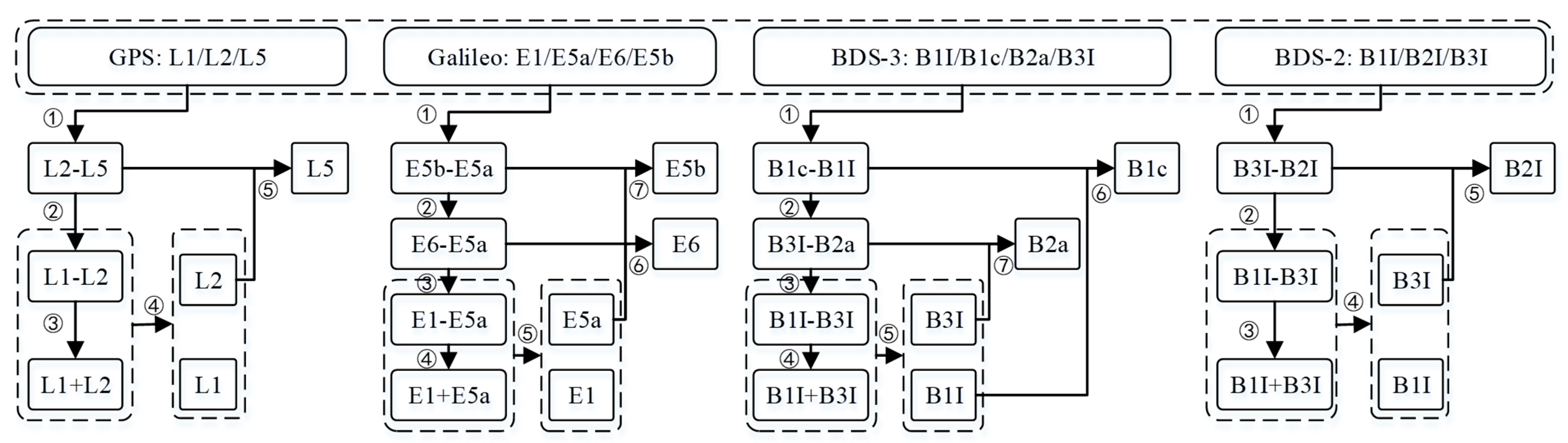
The multi-frequency FCB is usually estimated by the iterative least-squares method using globally distributed sites [34,35]. For multi-frequency uncombined PPP, the float ambiguity on each raw frequency can be directly used for FCB estimation in theory. However, in actual data processing, due to the short wavelength of the raw frequency, it is more sensitive to residual atmosphere error as well as to multipath and other unmodelled errors, thus its accuracy is poor. In this case, it might be down-weighted or rejected as gross errors in the quality control stage of FCB estimation, which in turn affects the estimation accuracy of FCB. In order to maximize the usage of float ambiguity and ensure the FCB accuracy, the float ambiguity on the raw frequency can generally be linearly transformed to form various combined ambiguities with excellent characteristics, such as long wavelength and weak ionosphere. Table 1 lists the EWL/WL combinations used in this article. In addition to the listed EWL/WL combinations, another linearly independent ambiguity combination needs to be selected. In this paper, in order to eliminate the influence of ionosphere delay, the NL ambiguity derived from the IF and WL ambiguity is selected as the last linear combination. Although its wavelength is only about 11 cm, it is hardly affected by the ionosphere.
According to the order of wavelength from largest to smallest, the EWL/WL/NL FCB is extracted in sequence. The specific steps are as follows:
- The EWL/WL float ambiguity is formed by the linear transformation of raw ambiguity and then the EWL/WL FCB is extracted using the least-squares method;
- In view of the long wavelength of WL ambiguity, by correcting WL FCB, the WL float ambiguity can be fixed by integer rounding;
- Construct IF float ambiguity from raw ambiguity, further combine the fixed WL ambiguity in the second step to calculate NL float ambiguity, and finally extract the NL FCB by the iterative least-squares method; and
The flowchart of the above multi-frequency FCB estimation algorithm is shown in Figure 1.
2.3. Multi-Frequency Stepwise Ambiguity Resolution
On the basis of the above function model and FCB product, in order to ensure the accuracy of extracted atmosphere information in the follow-up process, it is necessary to perform PPP AR first. For PPP AR, the FCB at the receiver end is first eliminated through the between-satellite-single-difference (BSSD) method and then the satellite FCB is corrected to restore the integer nature of ambiguity. Finally, the ambiguity is fixed as an integer through a certain function model, such as the widely used LAMBDA algorithm [37]. For uncombined multi-frequency high-dimensional ambiguity, it is extremely time-consuming to search and fix it as a whole. In addition, the significance of the ratio test decreases with the increase of the ambiguity dimension [38,39]. Therefore, in order to improve the AR efficiency, a stepwise AR method of fixing EWL/W/NL ambiguities sequentially is used in this paper. For the convenience of description, we take and as the raw frequency ambiguity and its variance–covariance matrix. By constructing a linear transformation matrix, the raw ambiguity can be mapped to EWL/WL/NL ambiguity and the corresponding variance–covariance matrix can also be obtained according to the variance–covariance propagation law.
where and represent the linear combination (LC) ambiguity and its variance–covariance matrix, and ,, are the mapping matrix from raw ambiguity to EWL/WL/NL ambiguity.
Then, the EWL/WL/NL ambiguity and its variance–covariance matrix is injected into the LAMBDA method sequentially to search for its optimal integer candidates. Take the multi-frequency observation of GPS L1/L2/L5, Galileo E1/E5a/E6/E5b, BDS-2 B1I/B2I/B3I, and BDS-3 B1c/B1I/B2a/B3I as an example; these are also the frequencies that will be used in the subsequent experiments of this article. The fixed EWL ambiguities in the first step include L2-L5 of GPS, E6-E5a/E5b-E5a of Galileo, B3I-B2I of BDS-2, and B1c-B1I/B3I-B2a of BDS-3. One thing to note is that although there are two EWL combinations for quad-frequency observations, they are all fixed simultaneously instead of being fixed in two steps. Then, the WL ambiguities of each system are fixed in the second step, including L1-L2 of GPS, E1-E5a of Galileo, and B1I-B3I of both BDS-2 and BDS-3. Finally, the NL ambiguities are attempted to be fixed, including L1 of GPS, E1 of Galileo, and B1I of both BDS-2 and BDS-3. In each step, if AR passes the ratio test, additional constraints can be used to update other parameters and then the multi-scale ambiguity-fixed solutions (EWL-fixed solution, WL-fixed solution, and NL-fixed solution) are obtained. In addition, the partial ambiguity resolution (PAR) strategy can be used in each step at the same time to improve the AR success rate [40,41].
2.4. Regional Atmosphere Modelling
Once NL ambiguity is fixed successfully, the ZWD and slant ionosphere delay can be updated through the fixed-minus-float ambiguity increments, as well as the corresponding variance–covariance matrix [42]. Based on the atmosphere information extracted at each reference station, the atmosphere at the user end can be interpolated according to its spatial distribution.
where and are indices for the user and reference stations; and are the interpolated ZWD and slant ionosphere delay; is the number of reference stations; and is the interpolation coefficient.
For a certain satellite, the ionosphere coefficients are usually calculated based on the difference between the ionospheric pierce point (IPP) coordinates of the user and reference stations.
where and are the differences between the latitude and longitude of IPP, respectively.
Similarly, the ZWD coefficients can be calculated by least-squares according to the differences of the Gaussian projection horizontal coordinates between the user and base stations, which can be found referring to Shi et al. [43].
where and denote the differences of the plane coordinates of the user and the reference stations.
After obtaining atmosphere information for users, the estimated parameters are constrained in the form of pseudo-observation equations to weaken their correlation, thereby shortening the initialization time. For the ZWD parameter, the constraint equation is as follows.
where represents the variance of ZWD information.
For the slant ionosphere information, as it is re-parameterized during the float PPP process, as shown in Equation (5), the interpolated value contains the receiver DCB of each reference station. Therefore, it cannot directly constrain the undifferenced ionosphere parameters. In order to eliminate the influence of the receiver DCB, the BSSD approach is adopted for the constraints of ionosphere parameters.
where and represent the un-reference and reference satellite, respectively, and represents the variance of BSSD ionosphere information.
3. Results
3.1. Data Processing
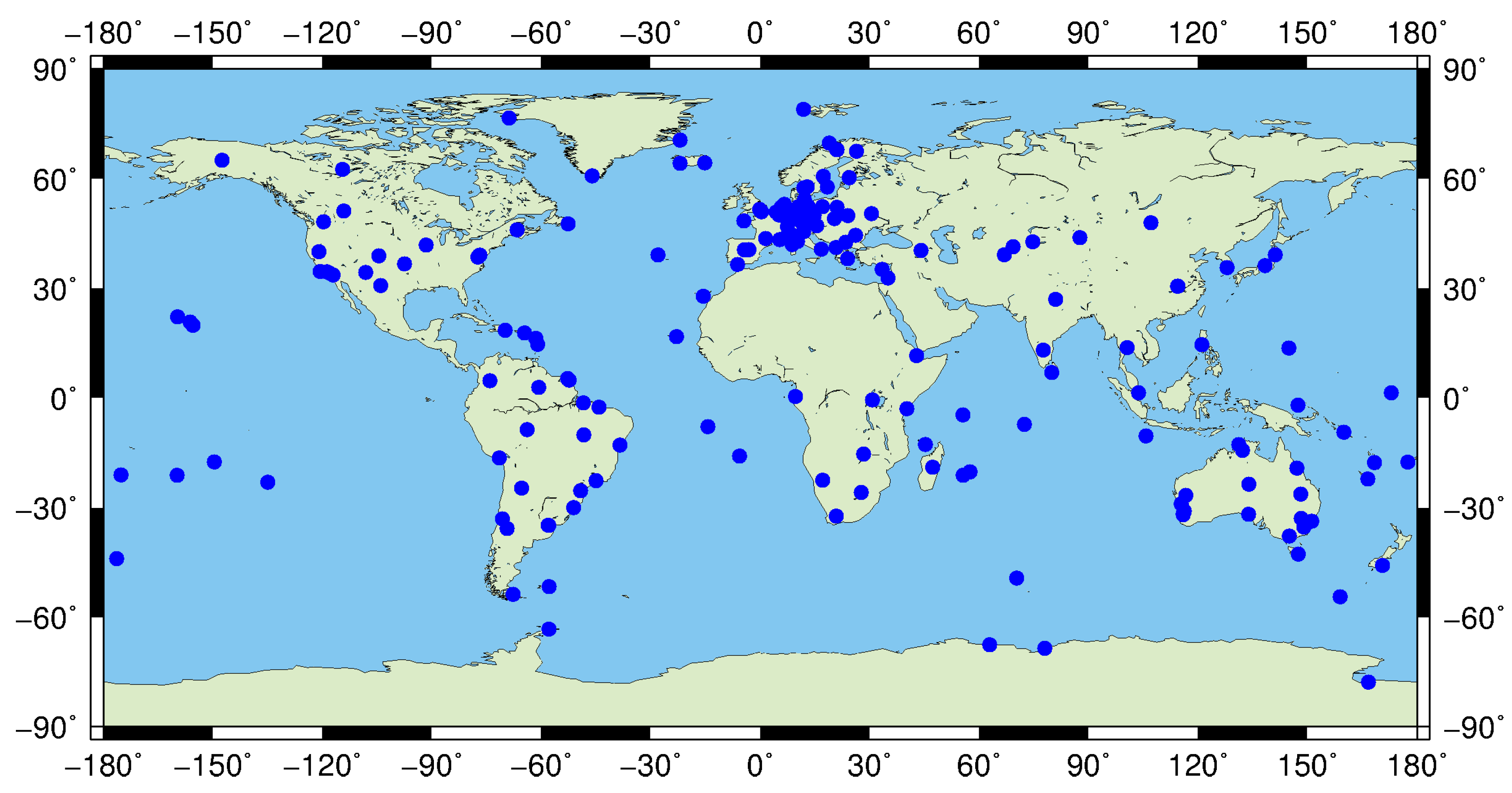
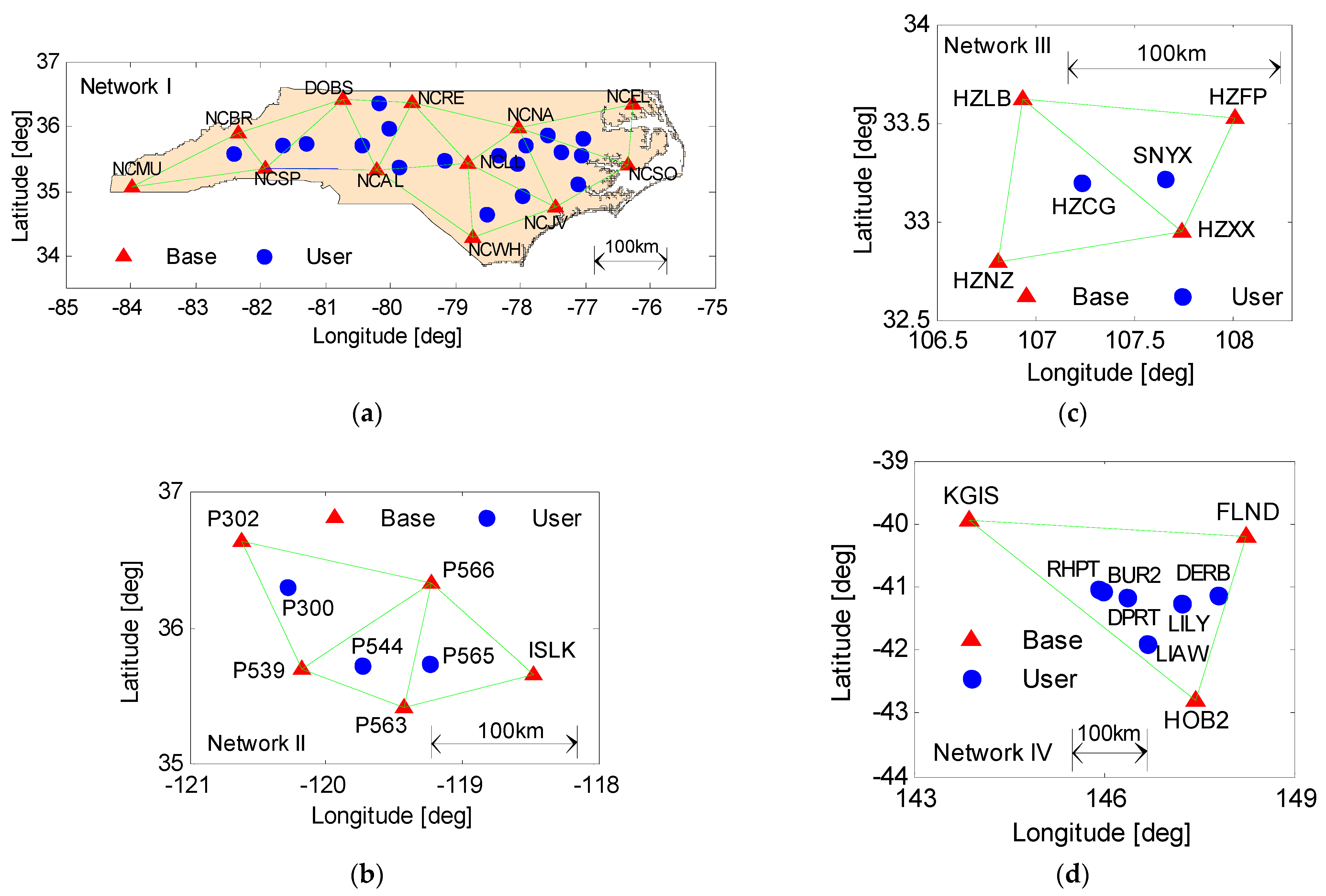
In order to verify the algorithm in this paper, experiments were carried out with various reference networks. Firstly, nearly 200 multi-GNSS experiment (MGEX) stations with 30 s sampling intervals distributed globally were used to extract multi-frequency FCB and their specific site distribution is shown in Figure 2. One thing to note is that due to the poor orbit accuracy of BDS GEO satellites, they are excluded from the FCB estimation process. Then, in order to analyze the influence of regional atmosphere modelling on single-epoch PPP AR, four groups of networks were selected for experiments. The specific site distribution is shown in Figure 3 and the detailed observation information of each dataset is shown in Table 2. In data processing, the cut-off elevation angle was set to 10° for usable measurements and an elevation-dependent weighting strategy was applied to both the raw phase and code measurements, with a priori precision of 3 mm and 0.3 m for IGSO/MEO satellites, while 1 cm and 1 m were used for GEO satellites, respectively. The rapid multi-GNSS orbit and clock products at intervals of 5 min and 30 s, respectively, provided by GeoForschungsZentrum Potsdam (GFZ), were used, wherein BDS-3 was processed with BDS-2 together using B1I/B3I observation types. We also applied the absolute phase centers model [26]. It is worth mentioning that due to lack of receiver PCO/PCV information for BDS and Galileo, we simply used GPS corrections instead. The elevation-dependent satellite-induced code biases of BDS-2 were also corrected according to Wanninger and Beer [44]. In addition, for multi-frequency pseudorange observations, the satellite DCB was corrected using products released by CAS, and for IFCB correction of multi-frequency phase observations, it was only applied for satellites of GPS Block IIF and BDS-2. In the process of AR, the well-known LAMBDA method was used to search for the optimal integer solution [37] and both stepwise AR and PAR strategies were adopted with a ratio threshold of 2.0. As for the regional atmosphere modelling, the Delaunay Triangulated Network (DTN) topology structure was adopted due to its uniqueness and efficiency. The following experiments were carried out from these three aspects: (1) results of multi-frequency FCB, (2) results of regional atmosphere modelling, and (3) results of single-epoch PPP AR. One thing to note is that, unlike the conventional filtering solution that uses multiple epoch data, in the single-epoch mode, it is generally considered that there is no relationship between adjacent epochs and all the estimated parameters in Equation (11) need to be reinitialized at each epoch. In the subsequent positioning experiments discussion, four types of single-epoch ambiguity-fixed solutions will be compared and for convenience of description, we refer to them as Solution A, Solution B, Solution C, and Solution D. The specific definitions are as follows:
- Solution A: conventional single-epoch WL ambiguity-fixed solution without atmosphere modelling;
- Solution B: single-epoch EWL ambiguity-fixed solution with atmosphere modelling;
- Solution C: single-epoch WL ambiguity-fixed solution with atmosphere modelling; and
- Solution D: single-epoch NL ambiguity-fixed solution with atmosphere modelling.
3.2. Results of Multi-Frequency FCB
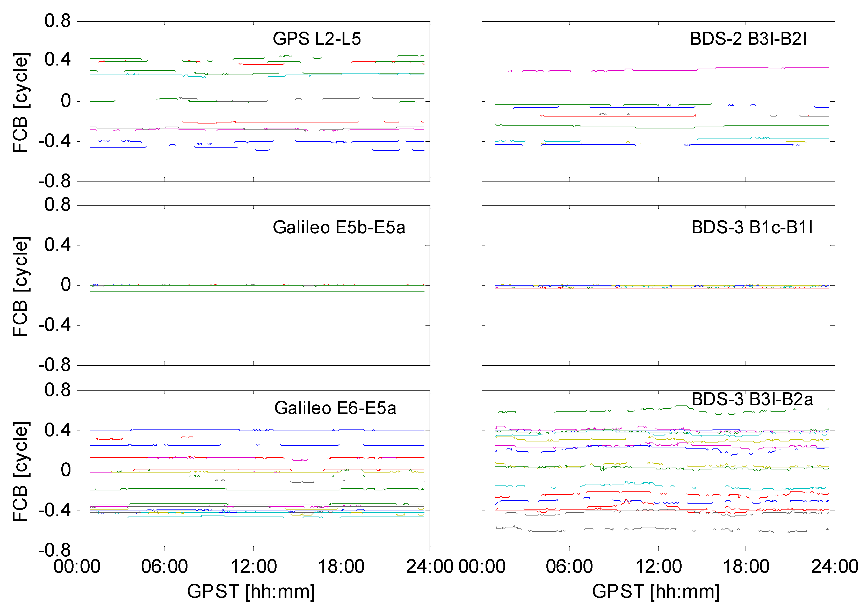
Using the FCB results of 2020 DOY148 as an example, Figure 4 shows the daily GPS/Galileo/BDS-3/BDS-3 EWL FCB series, wherein different colors indicate different satellites. In view of the long wavelength of EWL ambiguity, the EWL FCB of each system is very stable over time. At the same time, it is found that the values of Galileo E5b-E5a and BDS-3 B1c-B1I EWL FCB are very close to zero. Table 3 lists the specific statistical results of the daily standard deviation (STD) and it can be seen from the table that the average daily STD of EWL FCB was generally less than 0.02 cycles.
Figure 5 shows the WL and NL FCB series of GPS/Galileo/BDS-2/BDS-3. Table 4 also lists the STD statistics of each system. It can be found that the WL FCB of each system shows similar time-varying characteristics and changes were relatively stable within one day. Among them, the WL FCB of Galileo has the best stability, with an average STD of only 0.014 cycles. For NL FCB, its variation in a short period of time was small but due to its short wavelength, there were still certain fluctuations in one day. As for BDS-2, the stability of IGSO satellites was significantly better than that of MEO, with an average STD of 0.040 cycles and 0.170 cycles, respectively. This is mainly due to the poor spatial visibility of BDS-2 MEO satellites, especially outside the Asia–Pacific region. Compared with MEO, the IGSO satellites mainly served the Asia–Pacific region, with dense ground-tracking stations and more visible satellites per epoch, and this also means that its float ambiguity converged quickly and had high accuracy, thus it is reasonable that the FCB stability was better than for MEO. Overall, except for BDS-2 MEO satellites, the daily STD of NL FCB of each system generally did not exceed 0.1 cycles.
3.3. Results of Regional Atmosphere Modelling
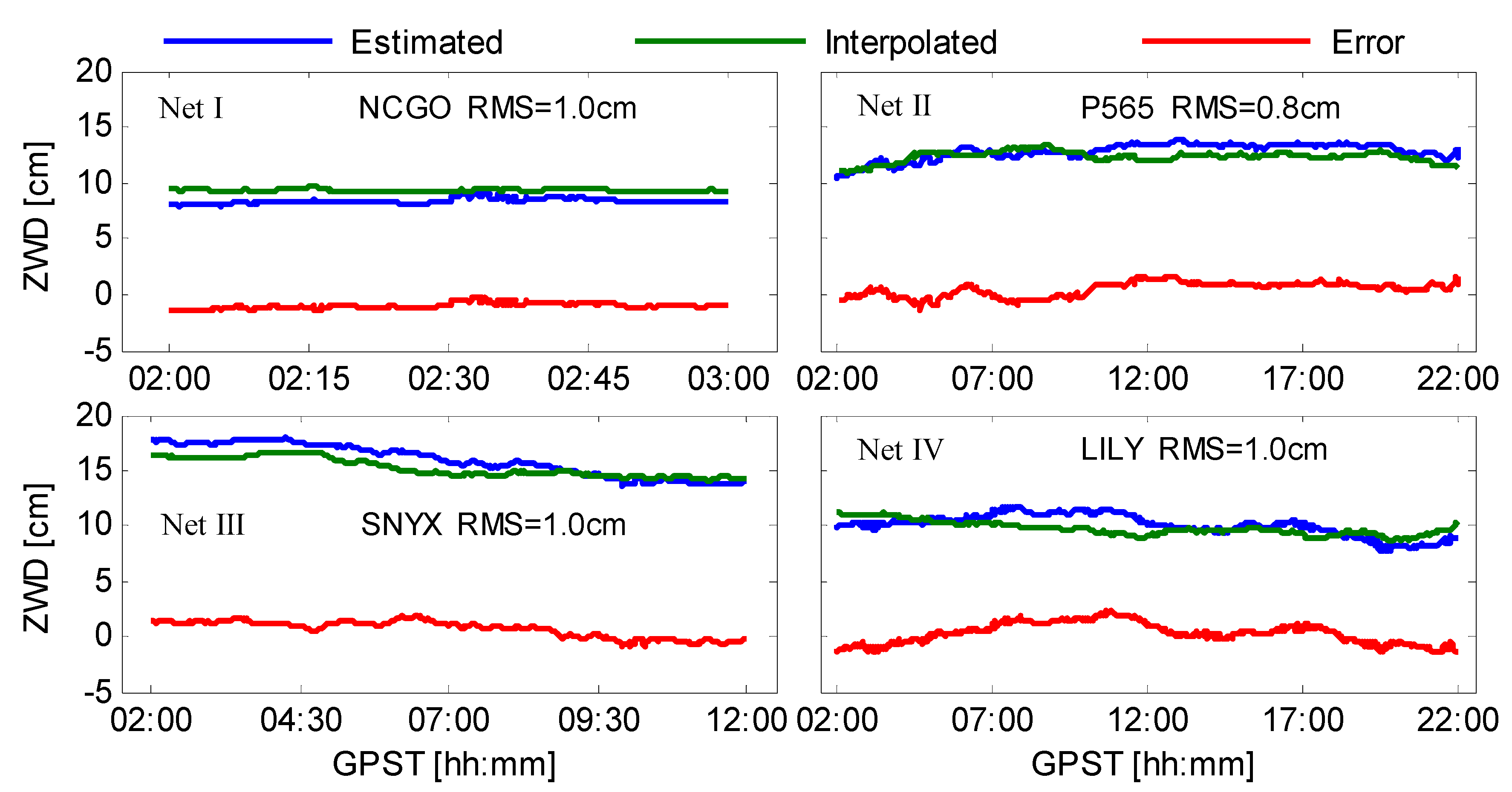
Four stations located in different networks are chosen as examples, namely NCGO, P565, SNYX, and LILY. Figure 6 shows the ZWD interpolation results. The magnitude of ZWD was about ten centimeters and changed slowly within a few hours. At the same time, it could be found that the difference between the interpolated value and the estimated value was small, and the ZWD interpolation accuracy of the four stations in the whole period was 1.0 cm, 0.8 cm, 1.0 cm, and 1.0 cm, respectively.
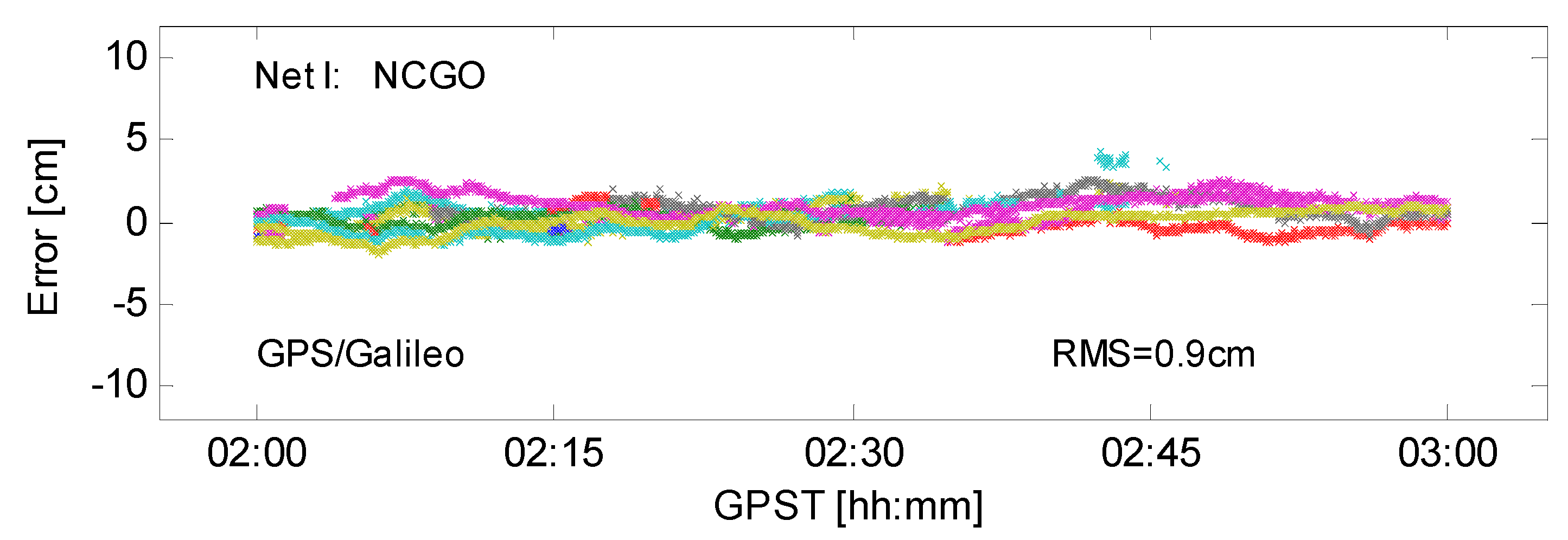
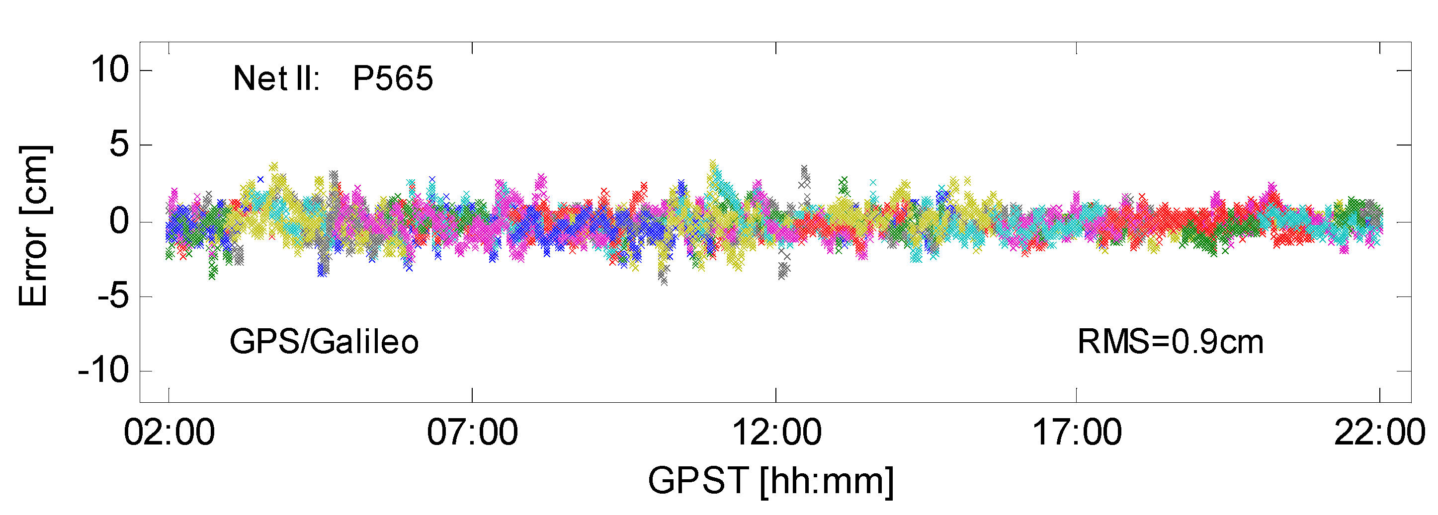
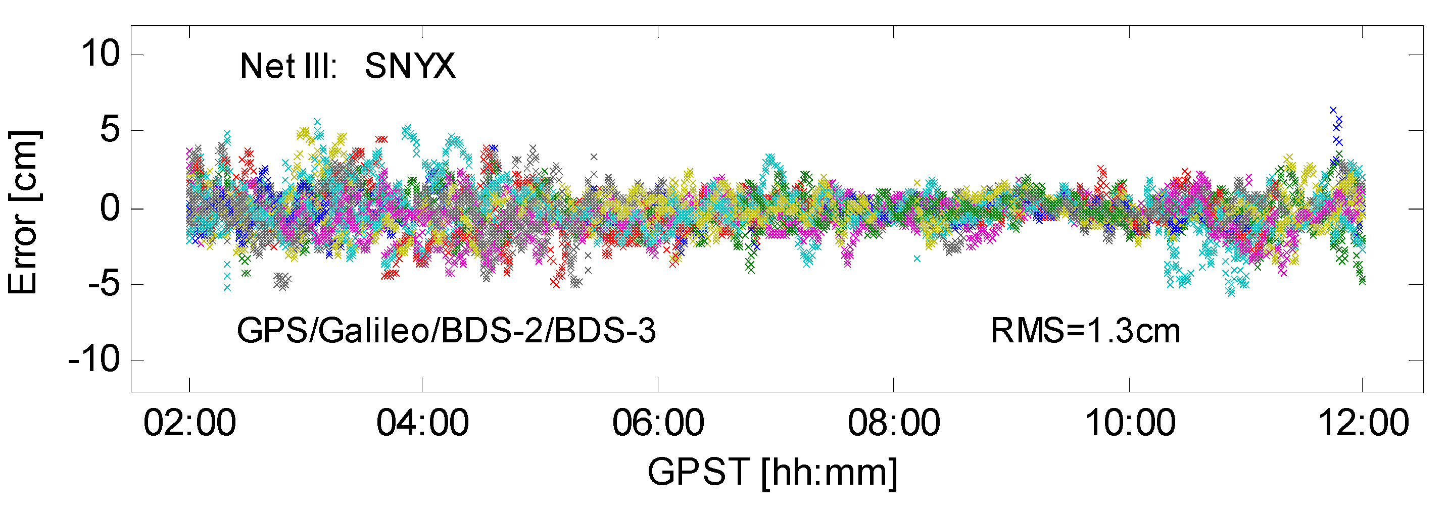
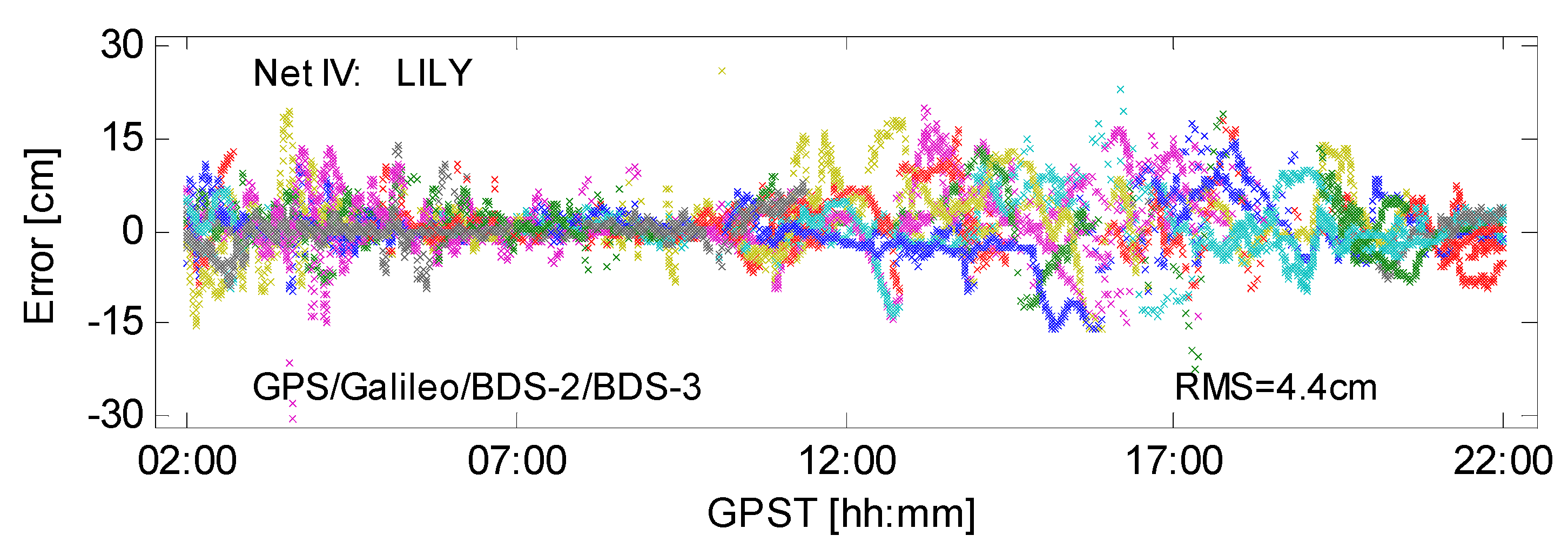
Figure 7, Figure 8, Figure 9 and Figure 10 show the BSSD ionosphere errors of these four stations and among them, different colors indicate different satellites. For station NCGO, P565, and SNYX, the interpolation error of each satellite generally did not exceed 5 cm. For the entire period, the interpolation accuracy was 0.9 cm, 0.9 cm, and 1.3 cm, respectively. The interpolation error of LILY was relatively large, even exceeding 15 cm in certain periods. The main reason for this phenomenon is that the average inter-distance of network I~III was within the range of about 90 km to 140 km, while the average inter-distance of network IV could reach about 369 km, as can be seen from Table 2. Generally speaking, the spatial correlation of atmosphere decreases as the distance between stations increases, thus the interpolation accuracy of LILY was relatively lower, and the RMS was only 4.4 cm.
Figure 11 further shows the atmosphere modelling results for all user stations. Overall, the interpolation accuracy of ZWD was better than that of the BSSD ionosphere. For network I~III, the average atmosphere modelling accuracy was better than 2 cm. Among them, the accuracy of ZWD was 0.5 cm, 0.8 cm, and 1.1 cm, respectively, and the accuracy of the BSSD ionosphere was 0.9 cm, 1.0 cm, and 1.6 cm, respectively. For network IV, due to its larger inter-station distance, the overall modelling accuracy was relatively lower, while the accuracy of ZWD and BSSD ionosphere was 1.7 cm and 5.2 cm, respectively.
3.4. Results of Single-Epoch PPP AR
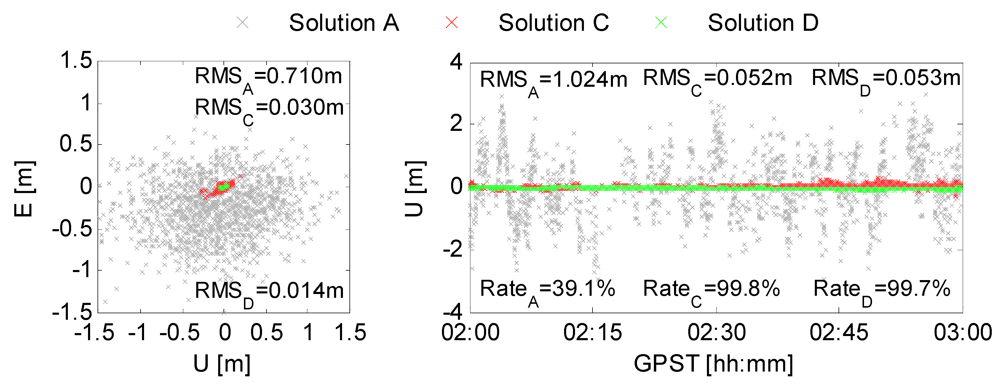
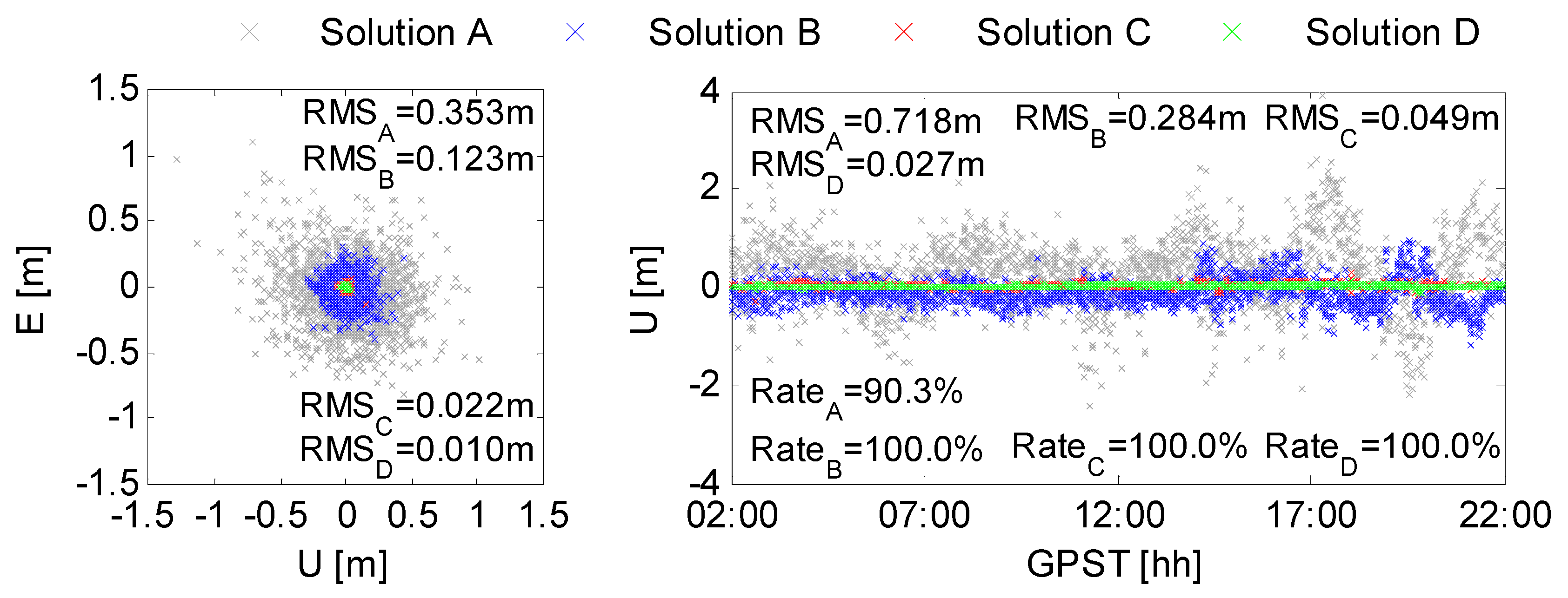
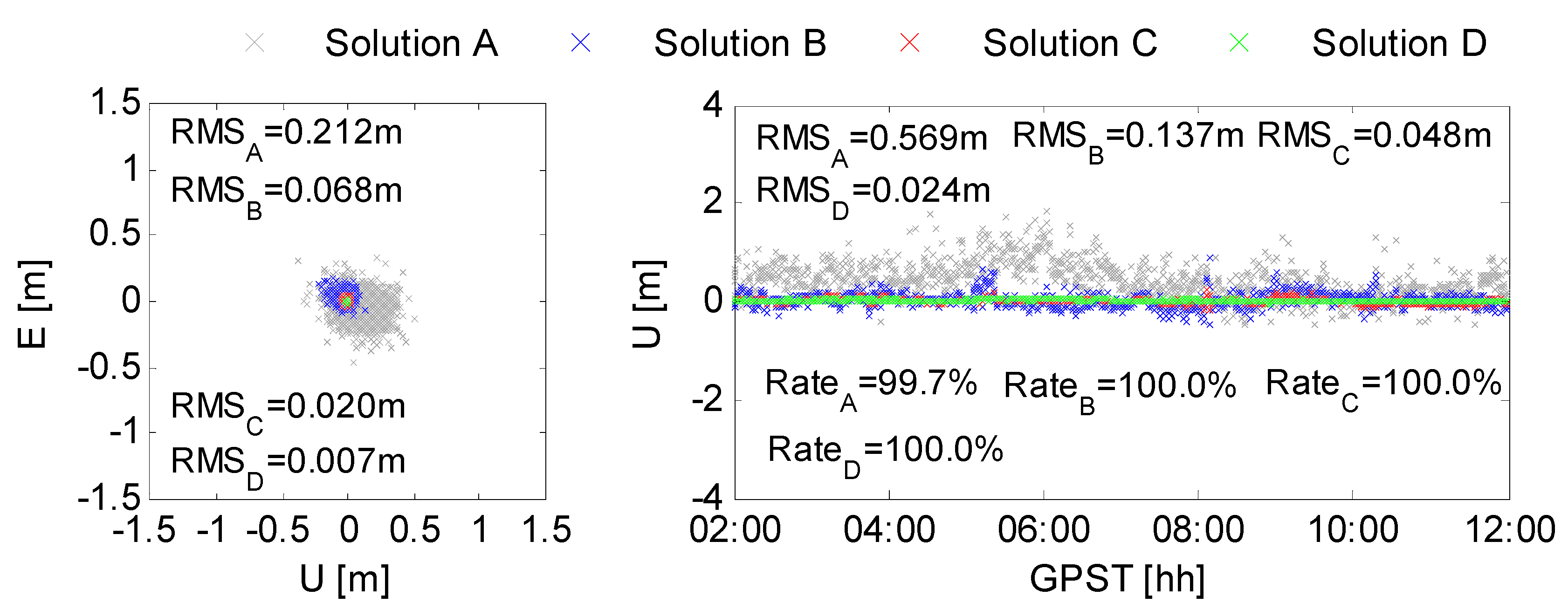
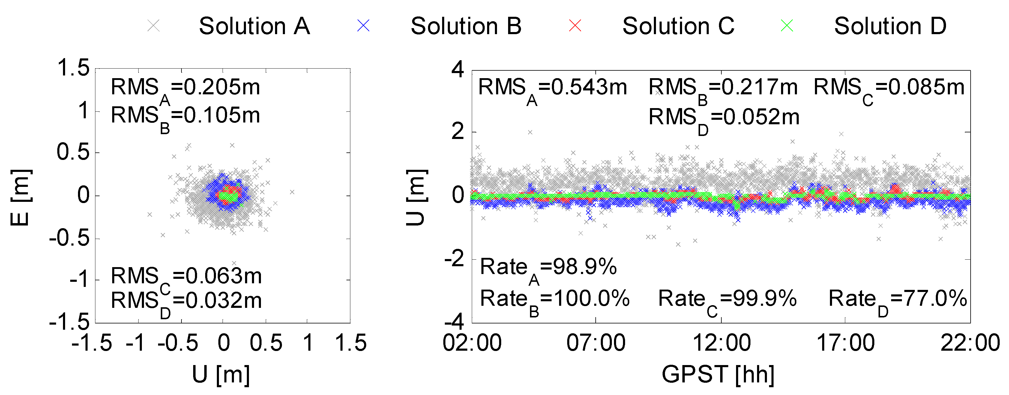
This section will analyze four types of single-epoch ambiguity-fixed PPP solutions. First, using NCGO, P565, SNYX, and LILY as examples, Figure 12, Figure 13, Figure 14 and Figure 15 directly compare the results of Solutions A~D. One thing to note is that the station NCGO can only receive GPS/Galileo dual-frequency data, thus there is no EWL ambiguity-fixed solution, namely Solution B. In comparing the results of different solutions at each station, a similar phenomenon can be seen, that is, the accuracy of the single-epoch EWL/WL/NL ambiguity-fixed solution with regional atmosphere modelling (i.e., Solutions B~D) was significantly better than that of the conventional WL ambiguity-fixed solution (i.e., Solution A).
In the conventional single-epoch mode (i.e., Solution A), in order to enhance the model strength, the atmosphere error is usually corrected by the empirical model. Due to limited correction accuracy, even if the WL ambiguity is successfully fixed, the positioning accuracy can only reach a few decimeters. Especially for station NCGO with only GPS/Galileo dual-frequency data, there was no EWL ambiguity constraint during the stepwise AR process, thus its positioning accuracy was the worst, with 0.710 m and 1.024 m in the horizontal and vertical direction, and the epoch fix rate was only 39.1%. In contrast, for stations P565, SNYX, and LILY, which could receive triple or quad-frequency data, under the constraints of EWL ambiguity, the conventional single-epoch WL ambiguity-fixed solution could also achieve a high epoch fix rate of 90.3%, 99.7%, and 98.9%, respectively. Meanwhile, the horizontal and vertical accuracy could be increased to about 20~35 cm and 50~70 cm, respectively.
In comparing the results of Solution A and Solution C, it can be clearly seen that with the addition of atmosphere constraints, the accuracy of the single-epoch WL ambiguity-fixed solution significantly improved from the decimeter level to several centimeters. Meanwhile, the epoch fix rate improved to varying degrees. Especially for dual-frequency data site NCGO, its horizontal and vertical accuracy increased to 0.030 m and 0.052 m, with an improvement of 95.8% and 94.9%, and the epoch fix rate also increased to 99.8%.
In further comparing the results of the single-epoch EWL/WL/NL ambiguity-fixed solution with regional atmosphere modelling (i.e., Solutions B~D), it can be found that the accuracy of the WL ambiguity-fixed solution was generally better than that of the EWL ambiguity-fixed solution and the accuracy of the NL ambiguity-fixed solution was higher than that of the WL ambiguity-fixed solution. The above phenomenon was mainly due to the different noise levels of EWL/WL/NL combinations. For the EWL/WL combination, in taking advantage of their long wavelength, the epoch fix rate close to 100% can usually be obtained. However, for the NL combination, although its accuracy was the best, fixing NL ambiguity successfully using only a single epoch of data requires sufficiently high-precision atmosphere modelling due to its short wavelength. From the analysis in Section 3.3 for network I~III, the overall modelling accuracy was better than 2 cm; thus, with high-precision atmosphere constraints, the single-epoch NL ambiguity-fixed solutions at NCGO, P565, and SNYX all achieved high epoch fix rates of 99.7%, 100.0%, and 100.0%, respectively. In contrast, for station LILY, due to the larger inter-station distance and lower modelling accuracy of network IV, the epoch fix rate of the NL ambiguity-fixed solution was only 77.0%.
Table 5 lists the accuracy results of all the user stations located in different networks and a similar phenomenon can be seen at different stations. The positioning performance of the single-epoch WL-fixed solution can be significantly improved with regional atmosphere constraints. For network I, the average horizontal and vertical accuracy increased from 70.1 cm and 98.0 cm to 2.8 cm and 4.5 cm, with an improvement of 96.0% and 95.4%, respectively. For network II~IV, due to the existence of EWL ambiguity constraints, the improvement was smaller than that in the dual-frequency case. The average horizontal accuracy increased from 41.3 cm, 22.0 cm, and 25.8 cm to 2.3 cm, 2.2 cm, and 7.7 cm, increased by 94.4%, 90.0%, and 70.2%, respectively. The average vertical accuracy increased from 80.5 cm, 54.6 cm, and 56.1 cm to 4.3 cm, 5.3 cm, and 9.8 cm, which were respectively increased by 94.7%, 90.3%, and 82.5%.
As for the accuracy of the single-epoch EWL/WL/NL ambiguity-fixed solution with atmosphere constraints (i.e., Solutions B~D), the horizontal and vertical accuracy of the EWL solution for different networks was about 6~15 cm and 20~30 cm, respectively. For network I~III, the WL solution achieved an accuracy of better than 3 cm and 5 cm in the horizontal and vertical direction, respectively. Due to the smaller noise level of the NL combination, its accuracy was generally better than the WL solution, and its average accuracy in the horizontal and vertical direction was better than 1.5 cm and 3.0 cm, respectively. For network IV with lower atmosphere modelling accuracy, the accuracy of the WL/NL solution was slightly worse than the other three networks. The average horizontal and vertical accuracy of the WL solution was 7.7 cm and 9.8 cm, respectively, and the corresponding results of the NL solution was 4.0 cm and 6.0 cm, respectively.
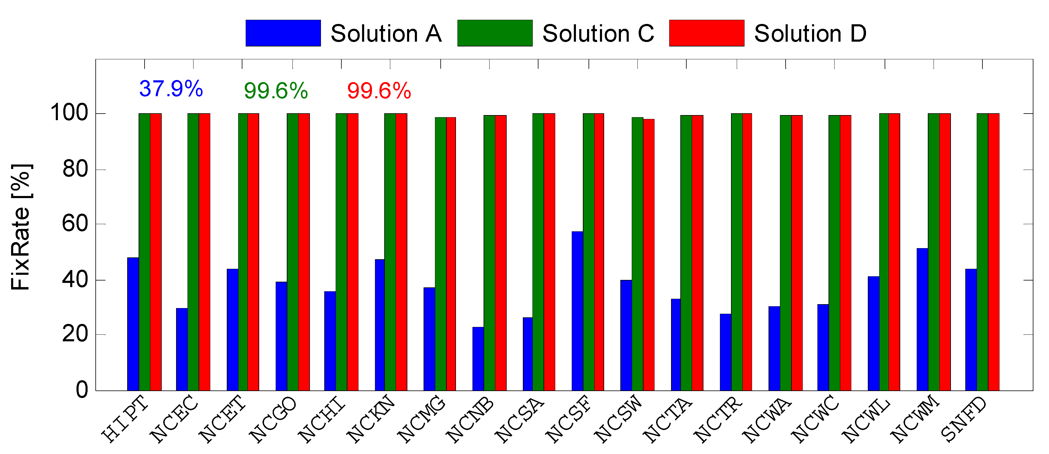
Figure 16 and Figure 17 further show the epoch fix rate of different ambiguity-fixed solutions. It can be seen from the figure that in view of the longest wavelength of EWL ambiguity, a fix rate of 100.0% can usually be achieved. As for the WL solution, in the case of dual-frequency, as shown in Figure 16, the epoch fix rate of the conventional WL solution was low, with an average value of only 37.9%. In contrast, after regional atmosphere modelling, the fix rate significantly improved, reaching 99.6%. For the case of multi-frequency, as shown in Figure 17, the fix rate of the WL solution only slightly improved after adding regional atmosphere constraints, and for network II~IV, it increased from 91.7%, 99.5%, and 96.2% to 99.9%, 100.0%, and 99.7%, respectively. In addition, it can also be seen from the figure that when the accuracy of regional atmosphere modelling is high enough, the NL ambiguity can also be successfully fixed. Among them, the epoch fix rate of network I~III could reach 99.6%, 99.9%, and 100.0%, respectively. However, when the atmosphere modelling accuracy is not accurate enough, it is difficult to fix NL ambiguity reliably (for example, the epoch fix rate of network IV was only 70.9%).
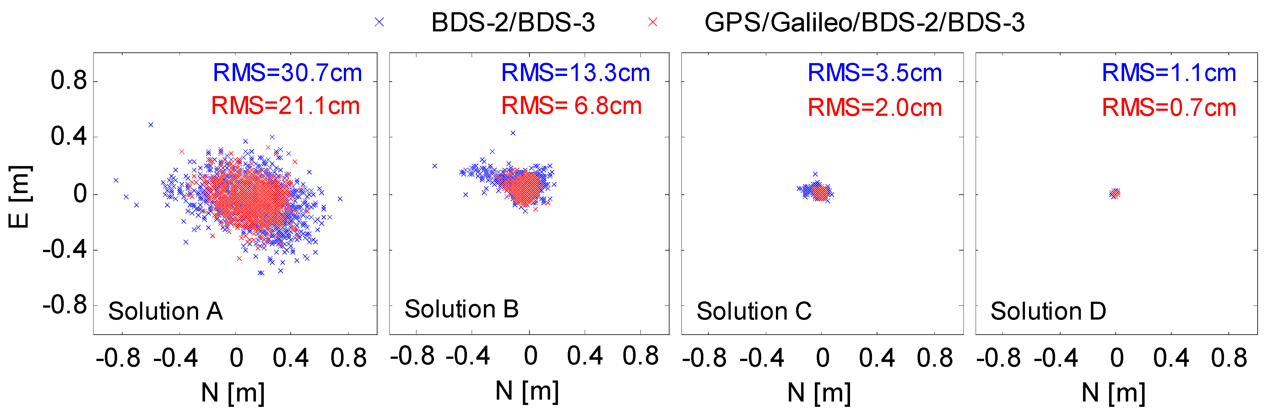
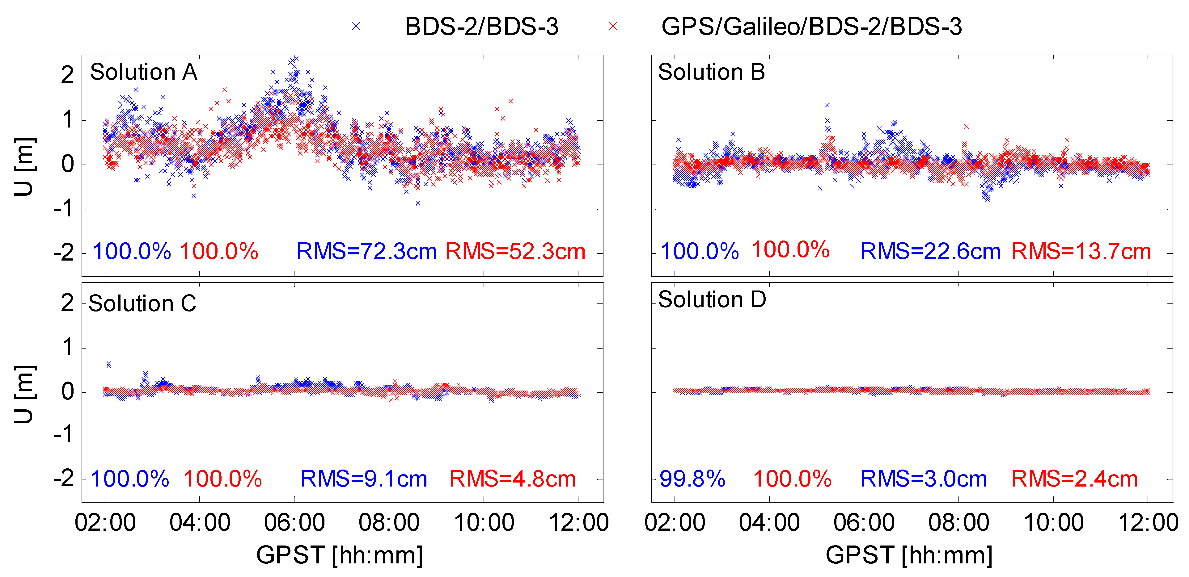
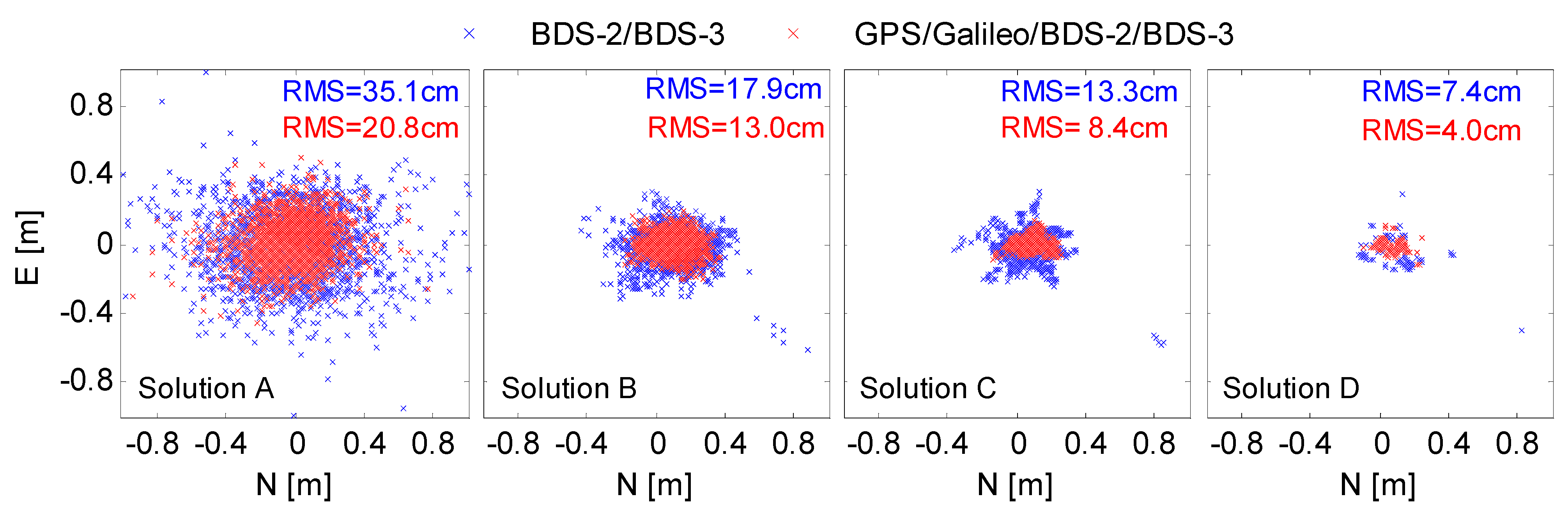
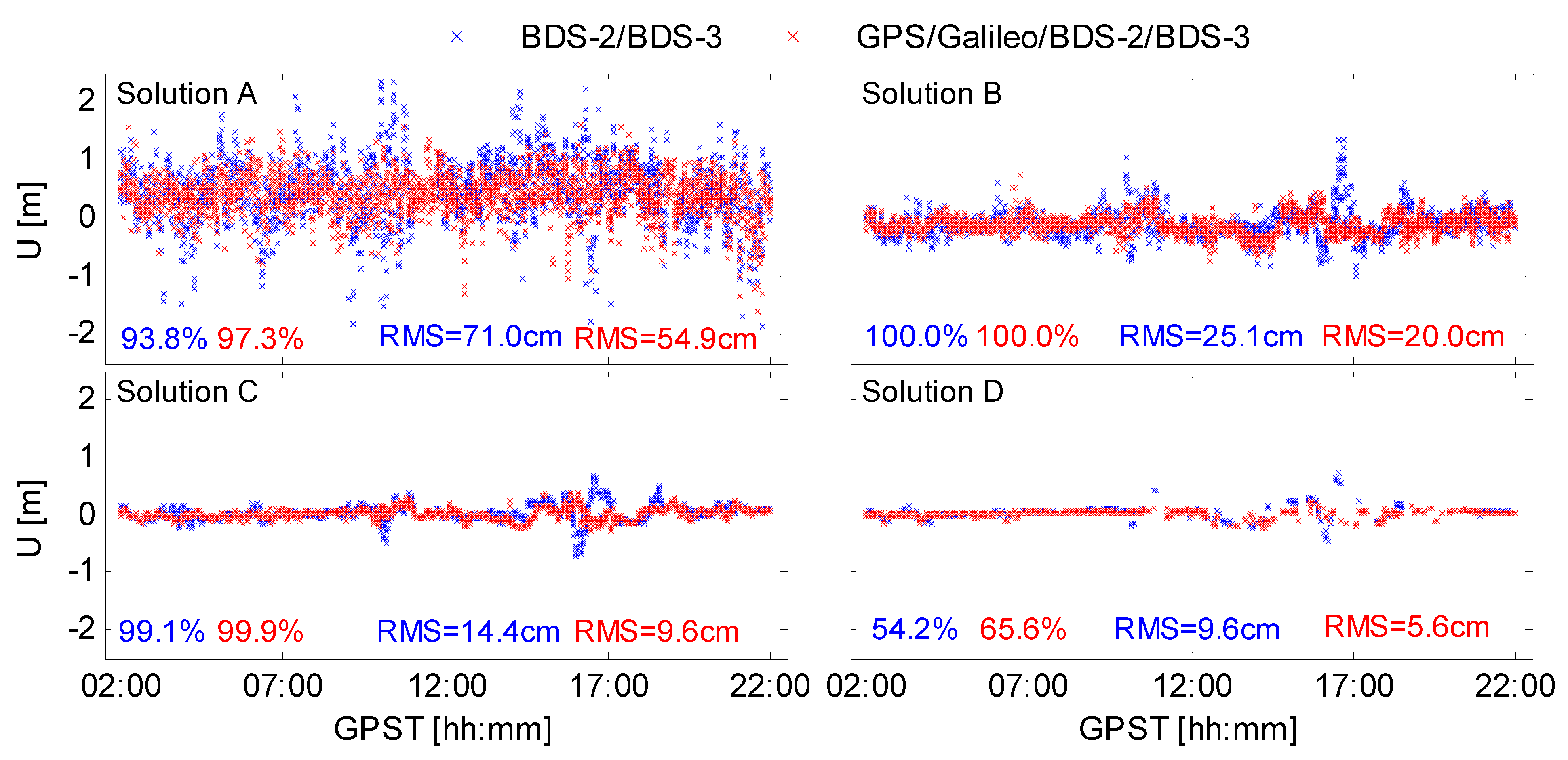
Using the SNYX and DPRT station as examples, the single-epoch PPP AR performance of BDS-only and multi-GNSS was further investigated and the results are shown in Figure 18, Figure 19, Figure 20 and Figure 21. In general, due to the better satellite spatial distribution and model strength of the multi-GNSS fusion, the error distribution was more concentrated than that of the BDS-only and both the positioning stability and accuracy improved. For station SNYX located in network III, the horizontal accuracy of Solutions A~D increased from 30.7 cm, 13.3 cm, 3.5 cm, and 1.1 cm to 21.1 cm, 6.8 cm, 2.0 cm, and 0.7 cm, which increased by 31.3%, 48.9%, 42.9%, and 36.4%, respectively. The vertical accuracy increased from 72.3 cm, 22.6 cm, 9.1 cm, and 3.0 cm to 52.3 cm, 13.7 cm, 4.8 cm, and 2.4 cm, with the improvement of 27.7%, 39.4%, 47.3%, and 20.0%, respectively. For station DPRT located in network IV, the horizontal accuracy increased from 35.1 cm, 17.9 cm, 13.3 cm, and 7.4 cm to 20.8 cm, 13.0 cm, 8.4 cm, and 4.0 cm, which increased by 40.7%, 27.4%, 36.8%, and 45.9%, respectively. The vertical accuracy increased from 71.0 cm, 25.1 cm, 14.4 cm, and 9.6 cm to 54.9 cm, 20.2 cm, 9.6 cm, and 5.6 cm, with the improvement of 22.7%, 19.5%, 33.3%, and 41.7%, respectively.
By further comparing the results of these two stations, it can be found that, regardless of the positioning accuracy or epoch fix rate, the results of DPRT were worse than that of SNYX, which was mainly caused by the lower accuracy of atmosphere modelling. For station SNYX, since the atmosphere modelling accuracy was high, even the NL solution of the BDS-only could reach a fix rate of 99.8%. In contrast, due to the limited accuracy of atmosphere modelling at station DPRT, the fix rate of the BDS-only NL solution was only 54.2%. It can be improved slightly and reach 65.6% through multi-GNSS combination. In general, reliable fixing of NL ambiguity in the single-epoch mode tightly depends on the regional atmosphere modelling accuracy.
4. Discussion
With the development of multi-GNSS and multi-frequency signals, the performance of PPP has been significantly improved in terms of the convergence time and positioning accuracy. Using these redundant signals, Li et al. [6], Guo et al. [7], Pan et al. [8], and Cao et al. [9] all proved that the convergence time can be generally shortened, from the traditional 20–30 min to less than 10 min. However, even so, the real-time property still cannot meet the needs of some industries, e.g., the self-driving vehicle. Thus, the single-epoch or nearly instantaneous PPP technology still are attractive and thereby it can be widely applied into various industries. Laurichesse and Banville [20] studied the instantaneous multi-frequency PPP using Galileo quad-frequency signals and the horizontal centimeter-level positioning could be obtained within about one minute. Geng et al. [21] studied the global instantaneous decimeter-level positioning using the multi-frequency single-epoch WL ambiguity-fixed solution. Considering the ionospheric error needs to be addressed through ionosphere-free combination, the observation noise is inevitably amplified. Although the decimeter-level accuracy may meet the requirement of many applications, the more precise, i.e., the centimeter or sub-decimeter level, demands still exist in many applications. For realizing this goal, high-precision atmosphere corrections seem indispensable, notably in NRTK as well.
Fast PPP with regional atmosphere enhancement was studied by Li et al. [24,25], wherein the successful NL AR was the prerequisite. Due to the short wavelength of NL ambiguity, reliable fixing of NL ambiguity using a single epoch of data tightly depends on the regional atmosphere modelling accuracy. Our study in this paper also indicates that it is difficult to fix NL ambiguity reliably in the single-epoch mode with a high fixing rate, especially for a network with long inter-station distance. Thus, for exploring more possibilities, four types of single-epoch PPP ambiguity-fixed solutions were analyzed, including the conventional single-epoch WL solution and regional atmosphere enhanced single-epoch EWL/WL/NL solutions. Through comprehensively considering the AR performance and positioning accuracy, we believe that the single-epoch WL solution with regional atmosphere modelling has a good development prospect for various positioning applications. Firstly, due to the addition of atmosphere constraints, its positioning accuracy is theoretically better than the conventional single-epoch WL solution with ionosphere estimation, which can reach centimeter to sub-decimeter levels. Secondly, the accuracy of the atmosphere modelling required for WL ambiguity-fixing is not as strict as for NL AR and thus the single-epoch fixing rate can be effectively guaranteed.
Concerning the comparison with the conventional NRTK technology, NRTK is also a high-precision positioning method based on the enhancement of the regional reference stations. In theory, under the support of the reference station network with the same density, the positioning performance of the two positioning technologies, i.e., NRTK and the single-epoch PPP with regional atmosphere enhancement, should be roughly the same. However, PPP technology realizes the decomposition of each error in the state domain, which makes some errors, such as satellite FCB, atmospheric delays, and other slowly varying or constant errors, become broadcasted at longer intervals. This can effectively reduce the amount of data transmission. In addition, the atmosphere-enhanced PPP model studied in this paper is consistent with the global PPP model. This means that the unity of wide-area and local-area positioning models is realized, and the two models can be seamlessly interchanged. Lastly, we believe that in NRTK positioning, the WL-fixed solution studied in this paper can also be similarly used in some applications, wherein a positive balance between real-time AR and positioning accuracy can be achieved.
5. Conclusions
The multi-system and multi-frequency provide new opportunities for the improvement of PPP performance. Based on a unified multi-frequency uncombined PPP model, this paper mainly focused on investigating the performance of single-epoch EWL/WL/NL AR with regional atmosphere modelling. Firstly, the function model of multi-frequency uncombined PPP was derived through the idea of re-parameterization. Then, based on the idea of linear transformation, the method of multi-frequency FCB estimation and the strategy of multi-frequency stepwise AR were introduced. Finally, on the basis of the NL ambiguity-fixed solution, the high-precision atmosphere at each reference station was extracted, further interpolated, and broadcast to users. By adding atmosphere constraints, the correlation between various parameters was significantly weakened so as to realize rapid PPP AR. In order to verify the above algorithm, the multi-frequency FCB was firstly extracted from globally distributed reference stations and its characteristics were analyzed. Then, four sets of reference networks with different sampling rates located in different regions were selected for experiments. The average distance between the reference stations was within the range of about 90 km to 369 km. Furthermore, the accuracy of the atmosphere modelling and performance of single-epoch PPP AR were analyzed.
In terms of multi-frequency FCB, the daily STD of EWL and NL FCB of each system generally did not exceed 0.02 cycles and 0.1 cycles, respectively. Among them, the value of Galileo E5b-E5a and BDS-3 B1c-B1I EWL FCB was almost zero. In terms of regional atmosphere modelling, the magnitude of ZWD was about a dozen centimeters and changed slowly with time. Overall, the modelling accuracy of ZWD was better than that of the BSSD ionosphere. For the reference network with an inter-station distance of about 90 km~140 km, the average modelling accuracy was better than 2 cm, and when the inter-station distance was expanded to about 369 km, the modelling accuracy of the ZWD and BSSD ionosphere decreased to 1.7 cm and 5.2 cm, respectively. In terms of the performance of single-epoch PPP AR, the conventional single-epoch WL solution usually used empirical models to correct atmosphere errors; due to the limited correction accuracy of the model, only decimeter-level accuracy could be obtained. Through regional atmosphere constraints, the positioning performance can be significantly improved and the corresponding accuracy can be increased to a few centimeters. In addition, the epoch fix rate can also be improved to varying degrees. Especially for the dual-frequency case, because there is no EWL ambiguity constraint in the stepwise AR process, the improvement was more obvious. With the addition of atmosphere constraints, the accuracy of the single-epoch EWL solution was about the decimeter level due to enlarged noise, while the WL/NL solution could achieve an accuracy of several centimeters. However, due to the short wavelength of NL ambiguity, reliable ambiguity-fixing tightly relies on high-precision atmosphere constraints. When the modelling accuracy was not accurate enough, it was difficult to fix NL ambiguity reliably in the single-epoch mode, although this situation can be improved to a certain extent through multi-GNSS combination. In contrast, the WL ambiguity can be successfully fixed and can still support the precise positioning with an accuracy of several centimeters.
Author Contributions
W.G. conceived the idea and designed the experiments with Q.Z. and S.P., W.G. and Q.Z. wrote the main manuscript. X.M. reviewed the paper. All components of this research study were carried out under the supervision of W.G. All authors have read and agreed to the published version of the manuscript.
Funding
This research study was funded by the National Natural Science Foundation of China (grant number 41904022, 41774027) and the Fundamental Research Funds for the Central Universities (2242021R41134).
Institutional Review Board Statement
Not applicable.
Informed Consent Statement
Not applicable.
Data Availability Statement
The multi-GNSS precise product provided by GFZ is available at ftp://ftp.gfz-potsdam.de/pub/GNSS/products/mgex/ (accessed on 1 September 2021). The MGEX DCB product provided by CAS is available at https://cddis.nasa.gov/archive/gnss/products/bias/ (accessed on 1 September 2021). The MGEX observation for multi-frequency FCB estimation is available at https://cddis.nasa.gov/archive/gnss/data/daily/ (accessed on 1 September 2021). The observation data in network I and II are available at https://geodesy.noaa.gov/corsdata/rinex/ (accessed on 1 September 2021). The observation data in network IV are available at ftp://ftp.data.gnss.ga.gov.au/daily/ (accessed on 1 September 2021). The observation data in network III are available upon request from the corresponding author considering it is not publicly available due to security issues.
Acknowledgments
The authors sincerely thank IGS (International GNSS Service), NGS (National Geodetic Survey), ARGN (Australian Regional GNSS Network), GFZ, and CAS for providing multi-GNSS data and products.
Conflicts of Interest
The authors declare no conflict of interest.
References
- Zumberge, J.F.; Heflin, M.B.; Jefferson, D.C.; Watkins, M.M.; Webb, F.H. Precise point positioning for the efficient and robust analysis of GPS data from large networks. J. Geophys. Res. Solid Earth 1997, 102, 5005–5017. [Google Scholar] [CrossRef] [Green Version]
- Kouba, J.; Héroux, P. Precise point positioning using IGS orbit and clock products. GPS Solut. 2001, 5, 12–28. [Google Scholar] [CrossRef]
- Tang, X.; Li, X.; Roberts, G.W.; Hancock, C.M.; de Ligt, H.; Guo, F. 1 Hz GPS satellites clock correction estimations to support high-rate dynamic PPP GPS applied on the Severn suspension bridge for deflection detection. GPS Solut. 2019, 23, 28. [Google Scholar] [CrossRef]
- Geng, J.; Teferle, F.N.; Shi, C.; Meng, X.; Dodson, A.H.; Liu, J. Ambiguity resolution in precise point positioning with hourly data. GPS Solut. 2009, 13, 263–270. [Google Scholar] [CrossRef] [Green Version]
- Zhang, X.; Li, P.; Guo, F. Ambiguity resolution in precise point positioning with hourly data for global single receiver. Adv. Space Res. 2013, 51, 153–161. [Google Scholar] [CrossRef]
- Li, X.; Ge, M.; Dai, X.; Ren, X.; Fritsche, M.; Wickert, J.; Schuh, H. Accuracy and reliability of multi-GNSS real-time precise positioning: GPS, GLONASS, BeiDou, and Galileo. J. Geod. 2015, 89, 607–635. [Google Scholar] [CrossRef]
- Guo, F.; Zhang, X.; Wang, J.; Ren, X. Modeling and assessment of triple-frequency BDS precise point positioning. J. Geod. 2016, 90, 1223–1235. [Google Scholar] [CrossRef]
- Pan, L.; Zhang, X.; Liu, J. A comparison of three widely used GPS triple-frequency precise point positioning models. GPS Solut. 2019, 23, 121. [Google Scholar] [CrossRef]
- Elsobeiey, M. Precise point positioning using triple-frequency GPS measurements. J. Navig. 2015, 68, 480–492. [Google Scholar] [CrossRef] [Green Version]
- Duong, V.; Harima, K.; Choy, S.; Laurichesse, D.; Rizos, C. An optimal linear combination model to accelerate PPP convergence using multi-frequency multi-GNSS measurements. GPS Solut. 2019, 23, 49. [Google Scholar] [CrossRef]
- Cao, X.; Li, J.; Zhang, S.; Kuang, K.; Gao, K.; Zhao, Q.; Hong, H. Uncombined precise point positioning with triple-frequency GNSS signals. Adv. Space Res. 2019, 63, 2745–2756. [Google Scholar] [CrossRef]
- Jin, S.; Su, K. PPP models and performances from single-to quad-frequency BDS observations. Satell. Navig. 2020, 1, 16. [Google Scholar] [CrossRef]
- Geng, J.; Bock, Y. Triple-frequency GPS precise point positioning with rapid ambiguity resolution. J. Geod. 2013, 87, 449–460. [Google Scholar] [CrossRef]
- Li, X.; Li, X.; Liu, G.; Feng, G.; Yuan, Y.; Zhang, K.; Ren, X. Triple-frequency PPP ambiguity resolution with multi-constellation GNSS: BDS and Galileo. J. Geod. 2019, 93, 1105–1122. [Google Scholar] [CrossRef]
- Li, X.; Liu, G.; Li, X.; Zhou, F.; Feng, G.; Yuan, Y.; Zhang, K. Galileo PPP rapid ambiguity resolution with five-frequency observations. GPS Solut. 2020, 24, 24. [Google Scholar] [CrossRef]
- Gu, S.; Lou, Y.; Shi, C.; Liu, J. BeiDou phase bias estimation and its application in precise point positioning with triple-frequency observable. J. Geod. 2015, 89, 979–992. [Google Scholar] [CrossRef]
- Li, P.; Zhang, X.; Ge, M.; Schuh, H. Three-frequency BDS precise point positioning ambiguity resolution based on raw observables. J. Geod. 2018, 92, 1357–1369. [Google Scholar] [CrossRef] [Green Version]
- Liu, G.; Zhang, X.; Li, P. Estimating multi-frequency satellite phase biases of BeiDou using maximal decorrelated linear ambiguity combinations. GPS Solut. 2019, 23, 42. [Google Scholar] [CrossRef]
- Geng, J.; Guo, J.; Meng, X.; Gao, K. Speeding up PPP ambiguity resolution using triple-frequency GPS/BeiDou/Galileo/QZSS data. J. Geod. 2020, 94, 6. [Google Scholar] [CrossRef] [Green Version]
- Laurichesse, D.; Banville, S. Innovation: Instantaneous Centimeter-level Multi-frequency Precise Point Positioning. GPS World 4 July 2018. Available online: https://www.gpsworld.com/innovation-instantaneous-centimeter-level-multi-frequency-precise-point-positioning/ (accessed on 1 September 2021).
- Geng, J.; Guo, J.; Chang, H.; Li, X. Toward global instantaneous decimeter-level positioning using tightly coupled multi-constellation and multi-frequency GNSS. J. Geod. 2019, 93, 977–991. [Google Scholar] [CrossRef] [Green Version]
- Geng, J.; Guo, J. Beyond three frequencies: An extendable model for single-epoch decimeter-level point positioning by exploiting Galileo and BeiDou-3 signals. J. Geod. 2020, 94, 14. [Google Scholar] [CrossRef]
- Guo, J.; Xin, S. Toward single-epoch 10-centimeter precise point positioning using Galileo E1/E5a and E6 signals. In Proceedings of the 32nd International Technical Meeting of the Satellite Division of The Institute of Navigation (ION GNSS+ 2019), Miami, FL, USA, 16–20 September 2019; pp. 2870–2887. [Google Scholar]
- Li, X.; Zhang, X.; Ge, M. Regional reference network augmented precise point positioning for instantaneous ambiguity resolution. J. Geod. 2011, 85, 151–158. [Google Scholar] [CrossRef]
- Li, X.; Huang, J.; Li, X.; Lyu, H.; Wang, B.; Xiong, Y.; Xie, W. Multi-constellation GNSS PPP instantaneous ambiguity resolution with precise atmospheric corrections augmentation. GPS Solut. 2021, 25, 107. [Google Scholar] [CrossRef]
- Schmid, R.; Steigenberger, P.; Gendt, G.; Ge, M.; Rothacher, M. Generation of a consistent absolute phase-center correction model for GPS receiver and satellite antennas. J. Geod. 2007, 81, 781–798. [Google Scholar] [CrossRef] [Green Version]
- Wu, J.T.; Wu, S.C.; Hajj, G.A.; Bertiger, W.I.; Lichten, S.M. Effects of antenna orientation on GPS carrier phase. Astrodynamics 1992, 1991, 1647–1660. [Google Scholar]
- Montenbruck, O.; Hugentobler, U.; Dach, R.; Steigenberger, P.; Hauschild, A. Apparent clock variations of the Block IIF-1 (SVN62) GPS satellite. GPS Solut. 2012, 16, 303–313. [Google Scholar] [CrossRef]
- Li, H.; Zhou, X.; Wu, B. Fast estimation and analysis of the inter-frequency clock bias for Block IIF satellites. GPS Solut. 2013, 17, 347–355. [Google Scholar] [CrossRef]
- Xia, Y.; Pan, S.; Zhao, Q.; Wang, D.; Gao, W. Characteristics and modelling of BDS satellite inter-frequency clock bias for triple-frequency PPP. Surv. Rev. 2020, 52, 38–48. [Google Scholar] [CrossRef]
- Pan, L.; Zhang, X.; Guo, F.; Liu, J. GPS inter-frequency clock bias estimation for both uncombined and ionospheric-free combined triple-frequency precise point positioning. J. Geod. 2019, 93, 473–487. [Google Scholar] [CrossRef]
- Wang, N.; Yuan, Y.; Li, Z.; Montenbruck, O.; Tan, B. Determination of differential code biases with multi-GNSS observations. J. Geod. 2016, 90, 209–228. [Google Scholar] [CrossRef]
- Zhou, F.; Dong, D.; Li, P.; Li, X.; Schuh, H. Influence of stochastic modeling for inter-system biases on multi-GNSS undifferenced and uncombined precise point positioning. GPS Solut. 2019, 23, 59. [Google Scholar] [CrossRef]
- Li, P.; Zhang, X.; Ren, X.; Zuo, X.; Pan, Y. Generating GPS satellite fractional cycle bias for ambiguity-fixed precise point positioning. GPS Solut. 2016, 20, 771–782. [Google Scholar] [CrossRef]
- Li, X.; Ge, M.; Zhang, H.; Wickert, J. A method for improving uncalibrated phase delay estimation and ambiguity-fixing in real-time precise point positioning. J. Geod. 2013, 87, 405–416. [Google Scholar] [CrossRef]
- Wang, J.; Huang, G.; Yang, Y.; Zhang, Q.; Gao, Y.; Xiao, G. FCB estimation with three different PPP models: Equivalence analysis and experiment tests. GPS Solut. 2019, 23, 93. [Google Scholar] [CrossRef]
- Temiissen, J.G. The least-squares ambiguity decorrelation adjustment: A method for fast GPS integer ambiguity estimation. J. Geod. 1995, 70, 65–82. [Google Scholar] [CrossRef]
- Verhagen, S.; Teunissen, P.J.G. The ratio test for future GNSS ambiguity resolution. GPS Solut. 2013, 17, 535–548. [Google Scholar] [CrossRef]
- Lu, L.; Ma, L.; Liu, W.; Wu, T.; Chen, B. A Triple Checked Partial Ambiguity Resolution for GPS/BDS RTK Positioning. Sensors 2019, 19, 5034. [Google Scholar] [CrossRef] [Green Version]
- Wang, J.; Feng, Y. Reliability of partial ambiguity fixing with multiple GNSS constellations. J. Geod. 2013, 87, 1–14. [Google Scholar] [CrossRef]
- Gao, W.; Gao, C.; Pan, S. A method of GPS/BDS/GLONASS combined RTK positioning for middle-long baseline with partial ambiguity resolution. Surv. Rev. 2017, 49, 212–220. [Google Scholar] [CrossRef]
- Dong, D.N.; Bock, Y. Global Positioning System network analysis with phase ambiguity resolution applied to crustal deformation studies in California. J. Geophys. Res. Solid Earth 1989, 94, 3949–3966. [Google Scholar] [CrossRef]
- Shi, J.; Xu, C.; Guo, J.; Gao, Y. Local troposphere augmentation for real-time precise point positioning. EarthPlanets Space 2014, 66, 30. [Google Scholar] [CrossRef] [Green Version]
- Wanninger, L.; Beer, S. BeiDou satellite-induced code pseudorange variations: Diagnosis and therapy. GPS Solut. 2015, 19, 639–648. [Google Scholar] [CrossRef] [Green Version]
Figure 1.
Flowchart of multi-frequency FCB estimation.

Figure 2.
Global MGEX stations distribution for multi-frequency FCB estimation.

Figure 3.
Four groups of reference network distributions with different inter-station distances: (a) network I located in North Carolina, USA, with GPS/Galileo dual-frequency data; (b) network II located in California, USA, with GPS/Galileo triple-frequency data; (c) network III located in Shaanxi, China, with GPS/Galileo/BDS-2/BDS-3 quad-frequency data; and (d) network IV located in Hobart, Australia, with GPS/Galileo/BDS-2/BDS-3 quad-frequency data.

Figure 4.
Daily EWL FCB series of GPS/Galileo/BDS-2/BDS-3 (2020 DOY148).

Figure 5.
Daily WL (left) and NL (right) FCB series of GPS/Galileo/BDS-2/BDS-3 (2020 DOY148).

Figure 6.
ZWD interpolation results of NCGO, P565, SNYX, and LILY.

Figure 7.
BSSD ionosphere interpolation errors of GPS/Galileo at station NCGO.

Figure 8.
BSSD ionosphere interpolation errors of GPS/Galileo at station P565.

Figure 9.
BSSD ionosphere interpolation errors of GPS/Galileo/BDS-2/BDS-3 at station SNYX.

Figure 10.
BSSD ionosphere interpolation errors of GPS/Galileo/BDS-2/BDS-3 at station LILY.

Figure 11.
Atmosphere modelling accuracy for all user stations.

Figure 12.
Single-epoch PPP ambiguity-fixed results at NCGO with GPS/Galileo dual-frequency data.

Figure 13.
Single-epoch PPP ambiguity-fixed results at P565 with GPS/Galileo triple-frequency data.

Figure 14.
Single-epoch PPP ambiguity-fixed results at SNYX with GPS/Galileo/BDS-2/BDS-3 quad-frequency data.
Figure 14.
Single-epoch PPP ambiguity-fixed results at SNYX with GPS/Galileo/BDS-2/BDS-3 quad-frequency data.

Figure 15.
Single-epoch PPP ambiguity-fixed results at LILY with GPS/Galileo/BDS-2/BDS-3 quad-frequency data.
Figure 15.
Single-epoch PPP ambiguity-fixed results at LILY with GPS/Galileo/BDS-2/BDS-3 quad-frequency data.

Figure 16.
Epoch fix rate of different ambiguity-fixed solutions in network I.

Figure 17.
Epoch fix rate of different ambiguity-fixed solutions in network II~IV (from left to right).
Figure 17.
Epoch fix rate of different ambiguity-fixed solutions in network II~IV (from left to right).

Figure 18.
Comparison of the horizontal positioning errors of the BDS-only and multi-GNSS single-epoch ambiguity-fixed solutions at station SNYX.
Figure 18.
Comparison of the horizontal positioning errors of the BDS-only and multi-GNSS single-epoch ambiguity-fixed solutions at station SNYX.

Figure 19.
Comparison of the vertical positioning errors of the BDS-only and multi-GNSS single-epoch ambiguity-fixed solutions at station SNYX.
Figure 19.
Comparison of the vertical positioning errors of the BDS-only and multi-GNSS single-epoch ambiguity-fixed solutions at station SNYX.

Figure 20.
Comparison of the horizontal positioning errors of the BDS-only and multi-GNSS single-epoch ambiguity-fixed solutions at station DPRT.
Figure 20.
Comparison of the horizontal positioning errors of the BDS-only and multi-GNSS single-epoch ambiguity-fixed solutions at station DPRT.

Figure 21.
Comparison of the vertical positioning errors of the BDS-only and multi-GNSS single-epoch ambiguity-fixed solutions at station DPRT.
Figure 21.
Comparison of the vertical positioning errors of the BDS-only and multi-GNSS single-epoch ambiguity-fixed solutions at station DPRT.


Table 1.
EWL/WL/NL combinations of GPS, Galileo, BDS-2, and BDS-3 for FCB estimation.
| System | Frequency | Wavelength/m | Tag | System | Frequency | Wavelength/m | Tag |
|---|---|---|---|---|---|---|---|
| GPS | L2-L5 | 5.86 | EWL | BDS-2 | B3I-B2I | 4.88 | EWL |
| L1-L2 | 0.86 | WL | B1I-B3I | 1.02 | WL | ||
| L1 + L2 | 0.11 | NL | B1I + B3I | 0.11 | NL | ||
| Galileo | E5b-E5a | 9.77 | EWL | BDS-3 | B1c-B1I | 20.93 | EWL |
| E6-E5a | 2.93 | EWL | B3I-B2a | 3.26 | EWL | ||
| E1-E5a | 0.75 | WL | B1I-B3I | 1.02 | WL | ||
| E1 + E5a | 0.11 | NL | B1I + B3I | 0.11 | NL |
Table 2.
Detailed information of the four sets of reference network data.
| # | Location | Average Inter-Station Distance | Time | Rate | Duration | Observation Type |
|---|---|---|---|---|---|---|
| I | North Carolina, USA | 139.1 km | 2020 DOY325 | 1 s | 1 h | GPS L1/L2 Galileo E1/E5a |
| II | California, USA | 102.6 km | 2020 DOY148 | 30 s | 20 h | GPS L1/L2/L5 Galileo E1/E5a/E5b |
| III | Shaanxi, China | 91.4 km | 2020 DOY148 | 30 s | 10 h | GPS L1/L2/L5 Galileo E1/E5a/E6/E5b BDS-2 B1I/B2I/B3I BDS-3 B1c/B1I/B2a/B3I |
| IV | Hobart, Australia | 369.5 km | 2021DOY182 | 30 s | 20 h | GPS L1/L2/L5 Galileo E1/E5a/E6/E5b BDS-2 B1I/B2I/B3I BDS-3 B1c/B1I/B2a/B3I |
Table 3.
Daily STD statistical results of GPS/Galileo/BDS-2/BDS-3 EWL FCB.
| STD (Cycle) | GPS L2-L5 | Galileo E5b-E5a | Galileo E6-E5a | BDS-2 B3I-B2I | BDS-3 B1c-B1I | BDS-3 B3I-B2a |
|---|---|---|---|---|---|---|
| Maximum | 0.014 | 0.002 | 0.007 | 0.015 | 0.003 | 0.025 |
| Minimum | 0.007 | 0.001 | 0.004 | 0.004 | 0.001 | 0.008 |
| Average | 0.011 | 0.002 | 0.005 | 0.008 | 0.002 | 0.016 |
Table 4.
Daily STD statistical results of GPS/Galileo/BDS-2/BDS-3 WL and NL FCB.
| System | WL FCB STD (Cycle) | NL FCB STD (Cycle) | |||||
|---|---|---|---|---|---|---|---|
| Maximum | Minimum | Average | Maximum | Minimum | Average | ||
| GPS | 0.070 | 0.021 | 0.041 | 0.116 | 0.028 | 0.062 | |
| Galileo | 0.022 | 0.010 | 0.014 | 0.115 | 0.048 | 0.076 | |
| BDS-2 | IGSO | 0.041 | 0.016 | 0.028 | 0.054 | 0.019 | 0.040 |
| MEO | 0.044 | 0.028 | 0.037 | 0.184 | 0.144 | 0.170 | |
| BDS-3 | 0.051 | 0.020 | 0.033 | 0.141 | 0.045 | 0.084 | |
Table 5.
Accuracy statistics of different types of single-epoch ambiguity-fixed PPP solutions.
| Site | Without Constraint | With Constraint | ||||||
|---|---|---|---|---|---|---|---|---|
| Solution A | Solution B | Solution C | Solution D | |||||
| H (cm) | V (cm) | H (cm) | V (cm) | H (cm) | V (cm) | H (cm) | V (cm) | |
| Network I with 139.1 km of inter-station distance 0.9 cm) | ||||||||
| HIPT | 74.9 | 88.2 | - | - | 2.3 | 3.8 | 0.6 | 1.2 |
| NCEC | 60.1 | 96.9 | - | - | 2.4 | 3.7 | 0.8 | 2.7 |
| NCET | 74.5 | 89.0 | - | - | 2.7 | 5.4 | 1.2 | 2.0 |
| NCGO | 71.1 | 102.4 | - | - | 3.0 | 5.2 | 1.4 | 5.3 |
| NCHI | 72.2 | 95.6 | - | - | 2.7 | 4.2 | 0.8 | 2.3 |
| NCKN | 63.0 | 93.0 | - | - | 2.6 | 5.1 | 1.6 | 3.8 |
| NCMG | 70.4 | 98.8 | - | - | 2.9 | 4.7 | 0.9 | 2.0 |
| NCNB | 70.6 | 108.7 | - | - | 3.4 | 4.7 | 0.7 | 1.1 |
| NCSA | 80.7 | 120.2 | - | - | 2.7 | 3.9 | 0.7 | 1.2 |
| NCSF | 52.9 | 82.0 | - | - | 2.9 | 4.4 | 2.0 | 2.9 |
| NCSW | 72.0 | 145.4 | - | - | 3.6 | 5.0 | 0.7 | 1.2 |
| NCTA | 80.0 | 96.3 | - | - | 3.0 | 3.8 | 0.7 | 1.9 |
| NCTR | 78.4 | 117.4 | - | - | 2.2 | 4.2 | 1.1 | 1.5 |
| NCWA | 87.0 | 90.4 | - | - | 3.1 | 4.8 | 0.6 | 1.9 |
| NCWC | 72.4 | 87.4 | - | - | 2.1 | 3.6 | 0.6 | 1.2 |
| NCWL | 71.5 | 88.6 | - | - | 3.1 | 4.0 | 0.7 | 3.6 |
| NCWM | 53.4 | 77.2 | - | - | 2.3 | 3.6 | 0.8 | 2.3 |
| SNFD | 57.4 | 86.9 | - | - | 4.0 | 6.2 | 1.8 | 1.5 |
| Average | 70.1 | 98.0 | - | - | 2.8 | 4.5 | 1.0 | 2.2 |
| Network II with 102.6 km of inter-station distance 1.0 cm) | ||||||||
| P300 | 46.2 | 93.6 | 12.5 | 28.1 | 2.6 | 4.1 | 1.2 | 2.1 |
| P544 | 42.5 | 76.2 | 13.9 | 30.0 | 1.8 | 4.0 | 1.1 | 2.0 |
| P565 | 35.3 | 71.8 | 12.3 | 28.4 | 2.3 | 4.9 | 1.0 | 2.7 |
| Average | 41.3 | 80.5 | 12.9 | 28.8 | 2.3 | 4.3 | 1.1 | 2.3 |
| Network III with 91.4 km of inter-station distance 1.6 cm) | ||||||||
| HZCG | 22.8 | 52.3 | 6.7 | 14.9 | 2.4 | 5.7 | 0.8 | 2.7 |
| SNYX | 21.2 | 56.9 | 6.8 | 13.7 | 2.0 | 4.8 | 0.7 | 2.4 |
| Average | 22.0 | 54.6 | 6.8 | 14.3 | 2.2 | 5.3 | 0.8 | 2.6 |
| Network IV with 369.5 km of inter-station distance 5.2 cm) | ||||||||
| BUR2 | 21.6 | 50.7 | 13.3 | 20.2 | 9.0 | 9.5 | 4.5 | 6.0 |
| DERB | 20.0 | 40.4 | 9.2 | 17.9 | 5.1 | 9.2 | 2.2 | 6.0 |
| DPRT | 20.8 | 54.9 | 13.0 | 20.2 | 8.4 | 9.6 | 4.0 | 5.6 |
| LIAW | 45.9 | 82.3 | 16.5 | 35.4 | 8.3 | 11.9 | 5.3 | 6.9 |
| LILY | 20.5 | 54.3 | 10.5 | 21.7 | 6.3 | 8.5 | 3.2 | 5.2 |
| RHPT | 26.1 | 53.7 | 13.9 | 20.8 | 9.2 | 10.0 | 4.7 | 6.5 |
| Average | 25.8 | 56.1 | 12.7 | 22.7 | 7.7 | 9.8 | 4.0 | 6.0 |
H and V represent the horizontal and vertical positioning accuracy, respectively. There are only GPS and Galileo dual-frequency data in Network I and thus the EWL results with Solution B are blank.
Publisher’s Note: MDPI stays neutral with regard to jurisdictional claims in published maps and institutional affiliations. |
© 2021 by the authors. Licensee MDPI, Basel, Switzerland. This article is an open access article distributed under the terms and conditions of the Creative Commons Attribution (CC BY) license (https://creativecommons.org/licenses/by/4.0/).
Share and Cite
MDPI and ACS Style
Gao, W.; Zhao, Q.; Meng, X.; Pan, S. Performance of Single-Epoch EWL/WL/NL Ambiguity-Fixed Precise Point Positioning with Regional Atmosphere Modelling. Remote Sens. 2021, 13, 3758. https://0-doi-org.brum.beds.ac.uk/10.3390/rs13183758
AMA Style
Gao W, Zhao Q, Meng X, Pan S. Performance of Single-Epoch EWL/WL/NL Ambiguity-Fixed Precise Point Positioning with Regional Atmosphere Modelling. Remote Sensing. 2021; 13(18):3758. https://0-doi-org.brum.beds.ac.uk/10.3390/rs13183758
Chicago/Turabian StyleGao, Wang, Qing Zhao, Xiaolin Meng, and Shuguo Pan. 2021. "Performance of Single-Epoch EWL/WL/NL Ambiguity-Fixed Precise Point Positioning with Regional Atmosphere Modelling" Remote Sensing 13, no. 18: 3758. https://0-doi-org.brum.beds.ac.uk/10.3390/rs13183758
Note that from the first issue of 2016, this journal uses article numbers instead of page numbers. See further details here.