Article

Landscape Structure and Seasonality: Effects on Wildlife Species Richness and Occupancy in a Fragmented Dry Forest in Coastal Ecuador

by
Xavier Haro-Carrión
1,2,3,4,*,
Jon Johnston
5 and
María Juliana Bedoya-Durán
2,3,6,7
1
Department of Geography, Macalester College, St. Paul, MN 55105, USA
2
Biodiversity Institute, University of Florida, Gainesville, FL 32611, USA
3
School of Natural Resources and Environment, University of Florida, Gainesville, FL 32611, USA
4
Department of Geography, University of Florida, Gainesville, FL 32611, USA
5
Wildlife Department, Humboldt State University, Arcata, CA 95521, USA
6
Department of Wildlife Ecology and Conservation, University of Florida, Gainesville, FL 32611, USA
7
Grupo de Investigación en Ecología Animal, Universidad del Valle, Cali 760021, Colombia
*
Author to whom correspondence should be addressed.
Remote Sens. 2021, 13(18), 3762; https://0-doi-org.brum.beds.ac.uk/10.3390/rs13183762
Submission received: 20 July 2021 / Revised: 13 September 2021 / Accepted: 16 September 2021 / Published: 19 September 2021
(This article belongs to the Special Issue Remote Sensing for Applied Wildlife Ecology)

Abstract

:
Despite high fragmentation and deforestation, little is known about wildlife species richness and occurrence probabilities in tropical dry forest (TDF) landscapes. To fill this gap in knowledge, we used a Sentinel-2-derived land-cover map, Normalized Difference Vegetation Index (NDVI) data and a multi-species occupancy model to correct for detectability to assess the effect of landscape characteristics on medium and large mammal occurrence and richness in three TDF areas that differ in disturbance and seasonality in Ecuador. We recorded 15 species of medium and large mammals, distributed in 12 families; 1 species is critically Endangered, and 2 are Near-Threatened. The results indicate that species occupancy is related to low forest cover and high vegetation seasonality (i.e., high difference in NDVI between the wet and dry seasons). We believe that the apparent negative effect of forest cover is an indicator of species tolerance for disturbance. The three sampling areas varied from 98% to 40% forest cover, yet species richness and occupancy were not significantly different among them. Vegetation seasonality indicates that more seasonal forests (i.e., those where most tree species lose their leaves during the dry season) tend to have higher mammal species occupancy compared to less seasonal, semi-deciduous forests. Overall, occupancy did not vary between the dry and wet seasons, but species-specific data indicate that some species exhibit higher occupancy during the wet season. This research offers a good understanding of mammal species’ responses to habitat disturbance and fragmentation in TDFs and provides insights to promote their conservation.

1. Introduction

Worldwide, biodiversity is declining at very high rates and land-cover change is considered the main driver [1,2,3]. The relationship between land-cover changes and biodiversity loss is particularly evident in tropical dry forests (TDFs) [4,5]. Globally, TDFs have been subject to intense forest clearing, with some regions of the world losing more than 80% of their estimated original TDF cover since 2001 [5]. The largest remnants of TDF are located in Latin America, a region where up to 40% of the original forest cover remains, but also the region where estimated deforestation (1980 to 2000) in TDFs is the highest [5]. Despite these high deforestation trends, TDFs are not well represented in conservation efforts in Latin America [6,7]. Particularly in the northwestern Pacific coast of South America, TDFs are estimated to be unprotected, highly fragmented and consequently at higher risk of human disturbance and further deforestation [6,7]. While these numbers call for increasing conservation efforts to protect remaining forests, they also suggest that a better understanding of human-impacted TDF landscapes is needed.
Anthropogenic land-cover changes often have significant impacts on wildlife communities [1,2,3,8,9]. Especially for large-bodied animals, habitat reductions ultimately cause local or regional extirpations or extinctions [8]. Most evidence suggests that Neotropical mammals are negatively affected by forest loss and fragmentation [10,11]. However, there are exceptions to this general trend, and some species will benefit and adapt to live in human-impacted landscapes [9,12,13]. The effect of land-cover on mammal species richness and abundance is probably higher in TDFs than in other more conserved environments. A study of various taxa suggests that given the large extent of human-dominated landscapes in Neotropical TDFs, the negative effects of land-cover change on local biodiversity will be among the highest in the globe [3]. Despite this trend, more localized studies show that significant numbers of species can persist in human-impacted ecosystems [9], suggesting the need for more research about wildlife persistence in human-impacted landscapes. In Ecuador’s TDFs, more than 70% of forests have been cleared [14,15], and many wide-ranging and keystone species have already been extirpated [16,17]; however, little is known about wildlife in the TDF fragments that persist [18,19].
In addition to high human impacts, TDFs in northwestern South America are seasonal, and mammals’ species numbers likely vary not only among forest types but also by seasons [20,21,22,23]. In TDFs in Colombia, detection probabilities have shown no variation across seasons, but the overall richness has been found higher in more deciduous forest types [22], and some species exhibited higher occurrence probabilities during months of lower precipitation [20]. In Ecuador, detection rates were higher in semi-deciduous tropical forests than in dry forests, but species richness values were similar [21]. These findings suggest that species richness and abundance patterns are likely influenced by both seasonality and forest type within TDFs. Thus, in order to better understand the effects of human impacts on mammal communities within highly fragmented TDFs, a detailed analysis of these factors in relation to anthropogenic land-cover change is necessary.
Wildlife inventories and monitoring, especially for medium and large-sized mammals, have evolved quickly from the use of indirect methods, such as transects, hair traps or footprint traps through the use of cameras. Camera traps underwent enormous advances and have been increasingly used in the last decade to gather information about different groups, including with notable success mammals, a group that tends to be highly elusive [24,25,26]. In addition, complex analytical methods, such as multi-species occupancy models, have been successfully used to analyze this type of information and offer multiple advantages over traditional methods. Advantages include the following: incorporation of uncertainty about detectability to overcome sampling biases related to the detection differences among species, improved occupancy estimations of rare or infrequent species, accurate calculations of community features by including potential undetected species and the inclusion of habitat covariates, such as detailed spatial and temporal information derived from remote sensing occupancy models are also ideal for dealing with small sample sizes. [27,28,29,30]. Remote sensing has been an important tool for wildlife management, especially for the conservation of large animals over extensive areas [31,32,33]. The recent availability of finer sensors and the development of advanced classification approaches has made the assessment of habitat quality for smaller areas possible [34]. From a conservation planning perspective, grouping spatially explicit information from multiple species is a powerful combination of tools, allowing us to understand species’ responses to changes in their landscapes and to accurately design management strategies according to the species realities [31,32,33].
This research focuses on understanding mammalian persistence and occurrence patterns in a highly fragmented landscape in central coastal Ecuador. We develop a hierarchical multi-species-occupancy model using detailed remote-sensing-derived covariates to investigate the influence of landscape characteristics on medium and large mammal occurrence probabilities and richness. We aim to fill gaps in the knowledge about wildlife species’ responses to significant human-driven changes in their habitats and to provide critical information about TDF wildlife species to enhance their conservation in fragmented landscapes.

2. Materials and Methods
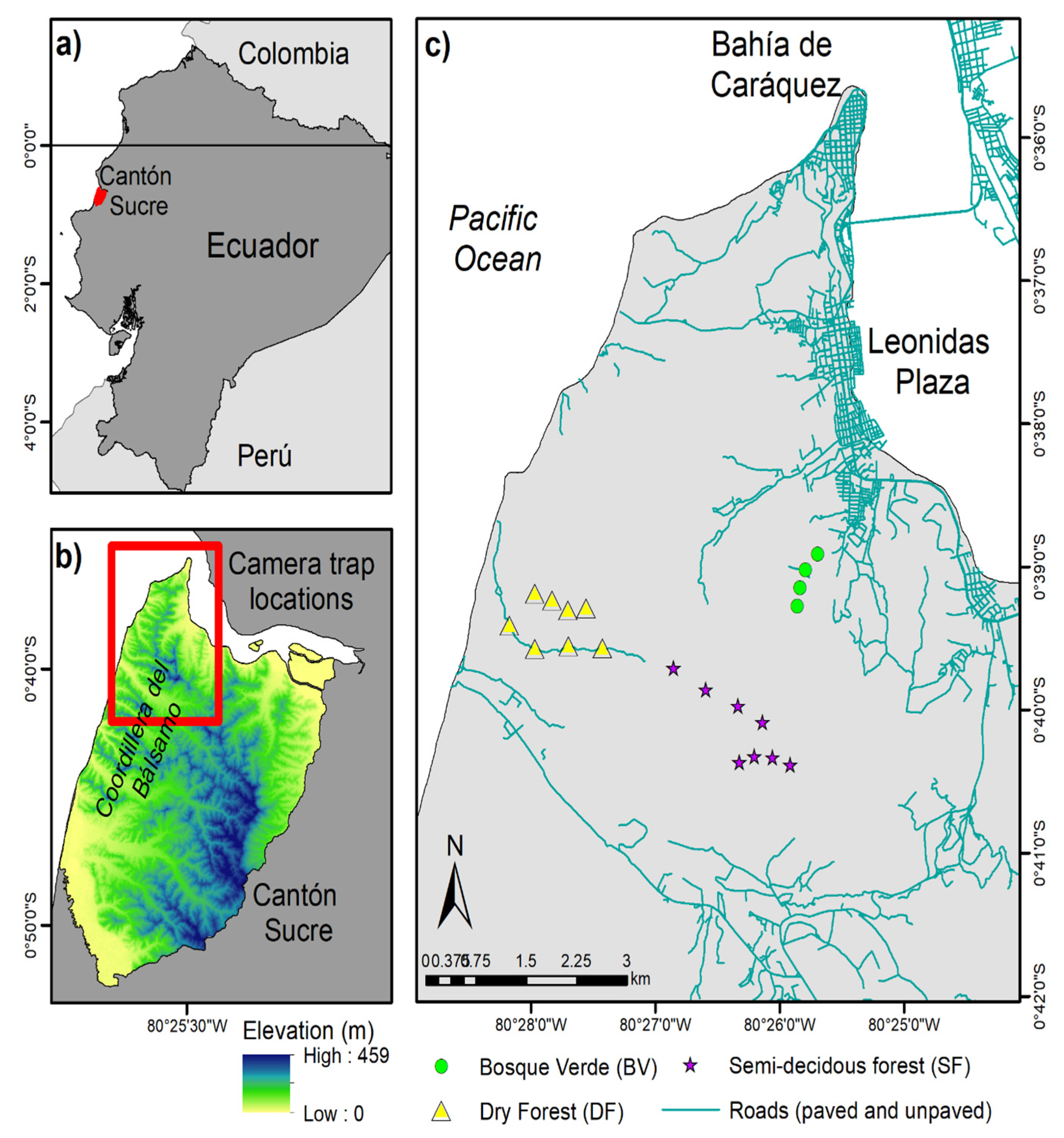
2.1. Study Area

The study landscape comprises Cantón Sucre, an area of about 39,875 ha located in Manabí province, central coastal Ecuador (Figure 1a,b). TDF formerly covered extensive areas of central coastal Ecuador, but most forests were cleared during the 1950s and 1960s [15], and recent estimates suggest that the few remnants left continue to be cleared at high rates [35]. The temperature fluctuates around 25 °C year-round. Precipitation is seasonal, around 450 mm annually, with 70% of it occurring between January and March and with a pronounced dry season of up to eight months. The months of lowest precipitation, typically July to September, could receive as low as 4 mm of monthly rainfall. (Data are derived from Climate Hazard Group InfraRed Precipitation with Station Data (CHIRP) between 2016−2019.) The northern part of Cantón Sucre is watered by the mouth of the Chone River, while the western part nears the Pacific Ocean. The coastline areas to the west quickly gain elevation inland, reaching almost 460 m at the highest point, forming a small chain of hills known as Coordillera del Bálsamo [36] (Figure 1b). Because of the low forest cover but high species diversity and endemism, this area is considered a biodiversity hotspot [37].
Wildlife sampling occurred in three areas in the Coordillera del Bálsamo section of the study landscape. The Bosque Verde (BV) reserve comprises approximately 20 ha of deciduous forest dominated by Ceiba trischistandra (Ceiba) trees. This site is estimated to be the most disturbed area because of its close proximity to the city of Leonidas Plaza. The other two areas are located inside the Punta Gorda reserve of about 50 ha, south and west of BV. The area more toward the coastline of the Punta Gorda reserve is also deciduous forest dominated by Ceiba trischistandra trees (hereof referred to as DF), while the area more toward the interior of the reserve is characterized by more semi-deciduous vegetation with various dominant canopy trees (hereof referred to as SF) (Figure 1c). Both of these reserves have been dedicated to conservation by private initiatives, and they are part of a network of approximately nine private reserves that joined efforts in the late 2000s to form corridors and promote biodiversity conservation in the area [36]. While small, we estimate these three sampling areas encompass all major variations in terms of vegetation phenology and human disturbance of the entire study landscape.

2.2. Camera Trapping

Camera-trapping was conducted from August 2016 to December 2017. Twenty Stealthcam G42 cameras were deployed across our three sampling areas. Eight cameras each were deployed within DF and SF areas, whereas 4 cameras were deployed in BV. Cameras were deployed along the linear geographical features, such as drainages and ridgelines, and were spaced 250−500 m apart, depending on accessibility. Fewer cameras were placed in BV mainly because the area was substantially smaller compared to DF and SF but also because it contained less geographic variation. In all cases, cameras were deployed along visible animal trails and attached to trees at an average height of 50 cm. Cameras were programmed to take 3 shots per trigger with a 5-s interval delay between triggers.
Cameras were checked on average every two weeks. During the wet season, weather conditions made it impossible to reach some cameras. Once accessibility was possible, we realized most cameras remained operational, but others had failed or had their view completely obstructed due to vegetation growth. Despite these problems, data from the wet season were included in our analyses, accounting for different sample sizes. Our survey period included the dry season of 2016 as well as both the wet and dry seasons of 2017. Sampling efforts over the entire survey period amounted to 6172 camera trap days. Total camera days reflect the total number of days that cameras were deployed and fully operational.
Photographs of mammal species were identified based on the Field Guide to the Mammals of Ecuador [38], and the taxonomic status was assigned according to the Mammals of Ecuador: updated species checklist [39,40]. Photographs of individual species were considered unique detections if they were separated from the previous detection by at least 24 h. For analyses of mammals, we included all species that triggered the cameras, except for small rodents, which were unidentifiable.

2.3. Landscape Characteristics
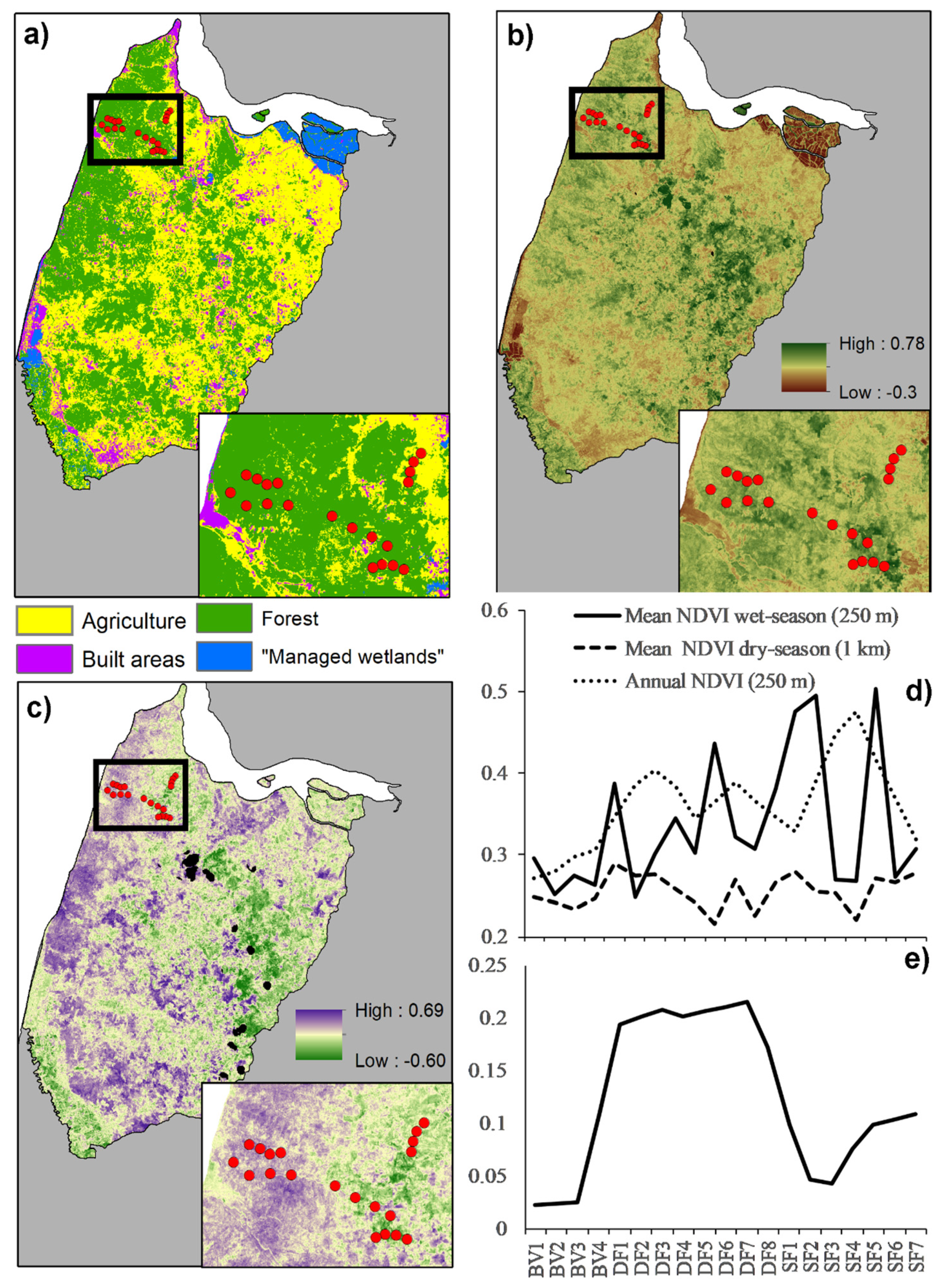
The following landscape characteristics were analyzed to understand the effect of human activities on wildlife species:

2.3.1. Land-Cover

We used Sentinel-2 data to classify the study landscape into forest, agriculture, built areas and managed wetlands, which are estimated to be the dominant landscapes of the study landscape. The forest class comprises evergreen and deciduous forests with various degrees of degradation, including some secondary regrowth. The agriculture class comprises annual crops and introduced pastures for cattle ranching. Built areas include human settlements, construction areas and paved roads. “Managed wetlands” refers to shrimp farms, rice fields or other managed ecosystems with a significant contribution of water in reflectivity. In general, pastures occur along major roads, forests occur adjacent to pasture in less accessible areas (including the coastline), built areas border pastures or occur scattered within them and “managed wetlands” border pastures in areas with high accessibility by the coastline.
Training data for classification analysis were obtained during field inventories conducted in July 2016. Additional training data for the built and managed-wetland classes were derived from Google Earth’s freely available high-resolution images. The built and “managed wetlands” classes were distinctive enough to be differentiated visually on Google Earth. A total of 82 training points were obtained for forest, 96 for agriculture, 53 for built areas and 40 for managed wetlands.
To obtain cloud-free composites for image classification, we masked out clouds from all Sentinel-2 images between January 2015 and December 2017 using the Sentinel-2 QA and Cirrus brands. We then created a single composite using the median value of each pixel. No major changes in land-cover were identified or reported during this time period. Additionally, spectral differences between land-cover types are estimated to be higher than seasonal differences within each class, making it possible to combine images from all months to create a cloud-free composite for land-cover classification.
We used Random Forest (RF) as a classification approach. RF is a machine learning technique that consists of tree-structured classifiers built by bootstrapped randomly selected predictors [41]. RF has been successfully used to classify complex landscapes in the humid and dry tropics [35,42,43]. Predictors for the RF classification included six Sentinel-2 bands, four band ratios, two vegetation indices and five image transformations (Table A1). We used 80% of the training data for classification analysis and 20% for accuracy assessment.

2.3.2. Forest Structure and Seasonality

We used the Normalized Difference Vegetation Index (NDVI), also derived from Sentinel-2 data, to characterize vegetation in terms of structure and seasonality. As a continuous index, NDVI provides details about vegetation not accounted for in the land-cover analysis.
We used the same process described in Section 2.3.1 to obtain cloud-composites but expanded the time frame to 2016−2020. This was conducted to reduce the potential effect of climate anomalies in the data and to increase the availability of cloud-free pixels for seasonal analyses. To estimate the vegetation structure, we calculated the mean-annual-NDVI for the 2016−2020 period. In vegetated areas, the maximum mean-annual-NDVI corresponds to mature forests, while the minimum mean-annual-NDVI corresponds to annual crops. Degraded forests, secondary forests and more seasonal forests will tend to have NDVI values closer to the maximum, while pastureland and annual crops values are closer to the minimum.
To characterize vegetation, especially forest, in terms of seasonality, we calculated the wet-season NDVI, dry-season NDVI and the difference between the wet and dry NDVI. We used annual precipitation occurring in each month to define seasons. We defined the wet season as that occurring between December and April and the dry season as that occurring between August and November. The remaining months were considered transitional and were excluded from this analysis. We calculated NDVI for each season and the difference between wet and dry-season NDVI. Non-seasonal vegetation, such as more mature and evergreen forests, was expected to exhibit similar NDVI values in both seasons and, therefore, a difference between seasons close to zero. Highly seasonal vegetation, such as deciduous forest, secondary forests and agriculture, was expected to be highly impacted by low precipitation and therefore exhibit significantly lower NDVI values during the dry season. In these cases, the difference between wet-season NDVI and dry-season NDVI will tend to be closer to one. All remote sensing analyses were performed using the Google Earth Engine (GEE).

2.3.3. Topography

Given the small size of the study landscape, we calculated the slope as the single most important predictor to topographically characterize the study landscape. We use the Shuttle Radar Topography Mission (SRTM, [44]) digital elevation data available in GEE.

2.4. Camera Trap Data Analysis

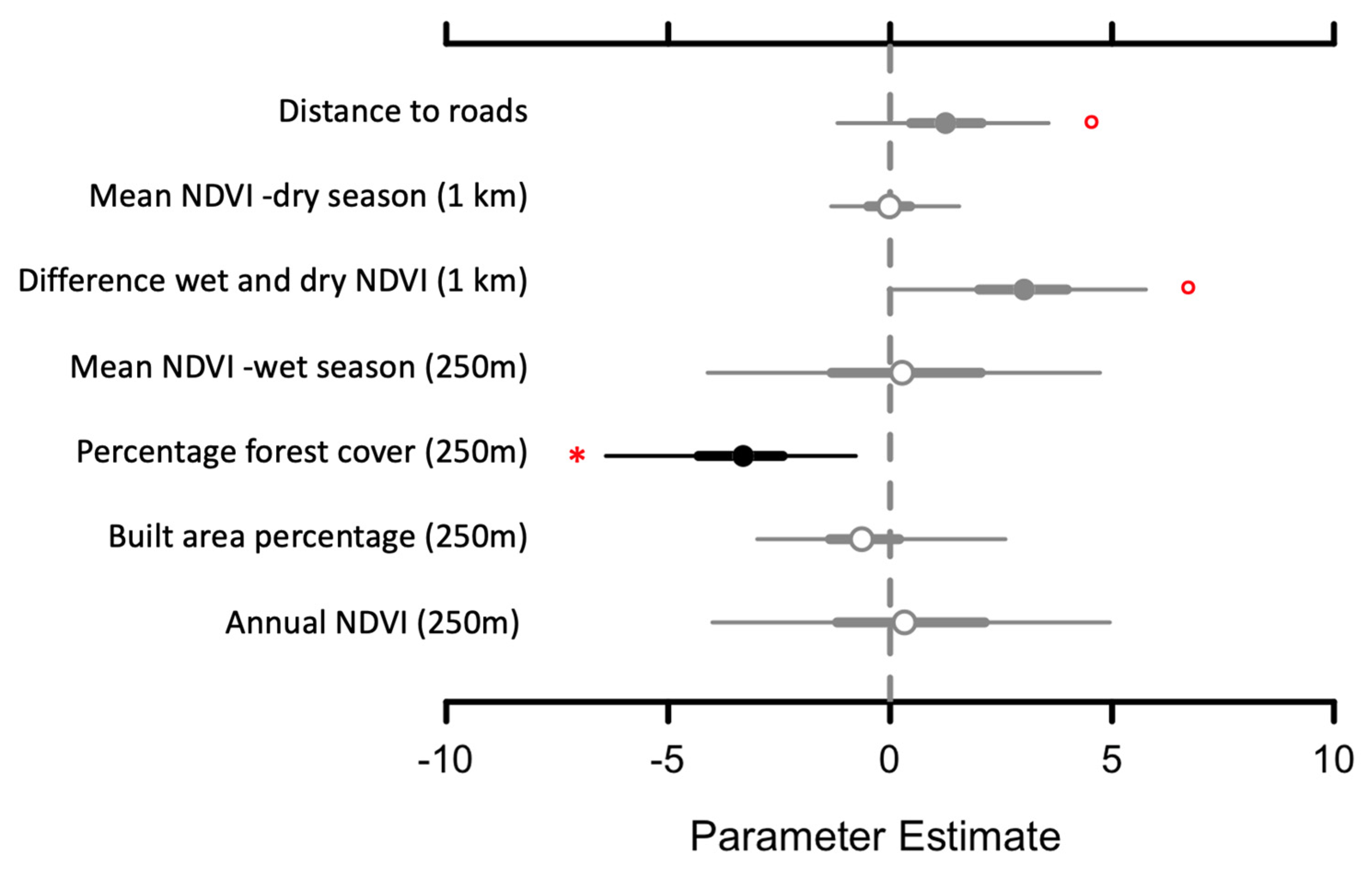
2.4.1. Model Predictors

The land-cover, annual-NDVI, wet-season-NDVI, dry-season-NDVI, difference between wet and dry NDVI maps and slope were used to calculate 16 landscape predictors. The percentage of forest, agriculture and built cover were calculated around each sampling site in 250 and 1000 m buffers. “Managed wetland”, which encompass rice fields and shrimp farms, was excluded because it does not represent a variable of importance to wildlife. The mean value of each NDVI metric and of the slope were also calculated for each buffer per sampling site. The sizes of the buffers were selected based on other similar studies [45,46] to estimate local-scale and broad-scale landscape characteristics. To further evaluate human impacts, we also calculated the shortest distance between each sampling site and paved or unpaved roads. From this pool of 17 predictors, the following seven uncorrelated predictors were selected as a predictor for occupancy models: percent forest cover in 1000 m buffers, percent built in 1000 m buffers, annual NDVI in 250 m buffers, wet-season NDVI in 250 m buffers, dry-season NDVI in 1000 m buffers, the difference between wet and dry season NDVIs in 1000 m buffers and distance to the road (paved and unpaved). When selecting uncorrelated predictors, we tried to include variables calculated at two buffer sizes to account for local and more broad geographic scales (See Table A2 for correlation of all variables). In addition to landscape variables, the presence of dogs, cattle and a slope (250 m) were also used to build the detection model. All variables included in the model were standardized (mean set equal to zero and variance equal to one) (Table 1).

2.4.2. Multispecies Occupancy Modeling

We used a multi-species occupancy framework with a Bayesian approach to calculate species occupancy and understand the influence of landscape predictors on species across the study landscape while accounting for detection biases during the sampling. We used this approach to improve species-specific estimates of occupancy [25,29,47]. To identify possible differences in terms of richness and occupancy between the two seasons, we assume two survey periods (dry and wet). We slightly modified the definition of seasons detailed in Section 2.3.2 to be able to include all camera trap data in our analysis. The months from January to mid-July were considered the “wet season”, while those between mid-July and December were the “dry season”.
We built the final model with the program JAGS [48] implemented in R, which uses Markov Chain Monte Carlo (MCMC) simulation to estimate parameters based on a posterior distribution. We used vague prior distributions for all parameters. We assessed convergence based on R-hat values < 1.1 [49]. We assessed the statistical significance of occupancy covariates based on whether 95% of credible intervals of beta estimates overlapped 0. For the analysis, we included all mammal species with at least 3 records.
To estimate the occurrence probability of each species at each sampling site, we included the predictors detailed in Section 2.4.1 using a logit link function. Each parameter was indexed by species and thus separately estimated for all the species present in the mammal community.

2.4.3. Analysis of Species Richness

To determine the pattern of terrestrial mammal richness across sampling sites, camera-level richness was calculated within the multi-species occupancy model using a data augmentation approach [27,28]. This data augmentation approach ensured that the number of all-zero detection histories was larger than the number of species that could have been missed in our sampling.
In addition, for sampling level richness, we used a rarefaction approach because the number of cameras differed across the three sampling areas and by seasons. These rarefaction analyses were performed using the R package iNEXT [50], which uses a bootstrap resampling method and extrapolation sampling curves to estimate an asymptotic species richness (bootstrap replicates = 100). As the input for our calculation of species richness, we used the median realized presence/absence (Z) matrix produced by the multi-species occupancy model, which is an estimate of the observed presence/absence matrix corrected for detection [27,29].

3. Results

3.1. Landscape Structure and Seasonality

The classification results highlight the human-impacted nature of the landscape. Forest accounted for only 42% of the landscape, while 58% encompassed anthropogenic land-cover types. Across the sampling areas, the percentage of forest cover in 1000 buffers was the lowest in BV (49%), followed by SF (81%) and DF (89%), suggesting a gradient of deforestation from BV to SF and DF. This trend persisted in 250 m buffers, indicating a similar landscape structure at both scales. Low forest cover means high agriculture cover as both variables are correlated (−0.98 1 k scale and −0.99 250 m). The percent of built in 1000 buffers exhibited a different pattern than that of forest. A higher percentage of built pixels were recorded in DF (3.6%), followed by SF (1.8%) and BV (1.5%), suggesting that, at least in small percentages at a scale of 1000 m around each site, there is no relationship between the presence of human settlements and forest cover. This trend is different at a scale of 250 m, where no built pixels were recorded in BV and DF, and a small percentage (1.3%) was recorded in SF (Figure 2a). Out-of-bag accuracy of 83% and Kappa of 0.75 indicate a reliable classification model (Table A3).
Normalized Difference Vegetation Index (NDVI) data provided critical details about the studied landscape, helping us to understand the broader implications of our findings and suggesting that BV, SF and DF are composed of different forest types. Annual NDVI data was the lowest in BV sites, followed by DF and SF at both 250 and 1000 m buffers. This pattern confirms our initial assumption when selecting sampling areas that SF is composed of more dense forests. DF is composed of less dense forest, while BV-NDVI reflects the high percentages of agriculture in this area (Figure 2a,b,d; Table 1).
Seasonal details of NDVI data provided further details about the landscape and the wildlife sampling areas. No differences were apparent between sampling areas in dry-season NDVI at either scale, 250 or 1000 m (Figure 2d). In contrast, wet-season NDVI patterns differed when analyzed at 250 and 1000 m. At 250 m, although the lowest wet-season NDVI was recorded in BV sites, many DF and SF sites exhibited similar values, indicating high within-sampling-area variation and little difference across sampling sites at this scale (Figure 2d). Significant seasonal differences became apparent when analyzing wet-season in 1000 m buffers and in the difference between wet and dry season NDVI. DF sites consistently showed higher NDVI values during the wet season at both scales, which translates into big differences in the NDVI between seasons in this sampling area. Apparently, DF sites are composed of highly seasonal forests followed, by far, by SF sites, which are likely composed of more evergreen vegetation. BV sites seem to have the lowest seasonality, but it is important to consider that high percentages of vegetation in BV sites, at least in the 1000 m buffer, were agriculture (Figure 2c,e; Table 1).

3.2. Wildlife Records

Overall, the total sampling effort yielded 835 independent records, 654 records from the dry season and 181 records from the wet season. A total of 15 species of mammals from 12 taxonomic families were documented. Of the species recorded, one is classified as critically endangered, and two are classified as near threatened at the global level in the IUCN Red List [51]. At the national level, one species is classified as Critically Endangered, one species is classified as Endangered, one species is classified as Near-Endangered, two species are classified as Vulnerable, and four species are classified as Near-Threatened in the Red Book of Mammals of Ecuador [39] (Table 2).

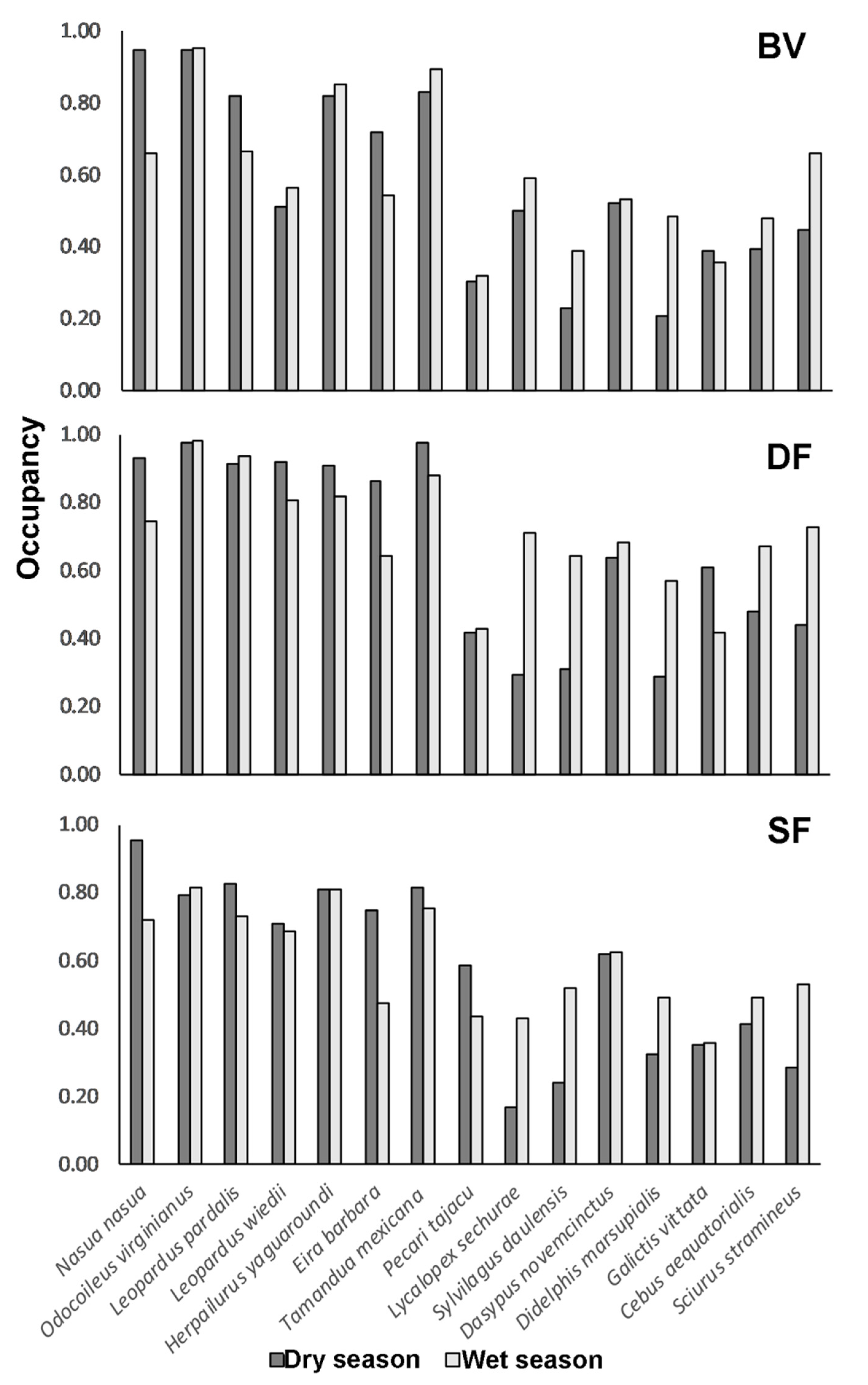
3.3. Species Occupancy and Richness

We did not find differences in richness at the camera (Figure 3a) level among sampling areas and between seasons, but a slightly higher mean richness was found at DF during the dry (Species richness = 10 with confidence intervals (CI): 7.3–13.4) and wet seasons (Species richness = 10.8 with CI: 7.6–14.4) than in the two other forest types. When calculating community-level estimates, we detected that both Shannon and Simpson diversity estimates for DF were greater especially compared to SF (No overlap between them) and in lower proportion to BV. However, confidence intervals for BV suggest more uncertainty in the prediction for both indexes (Figure 3b).
The mean response of species occupancy was significantly negative (CI did not overlap zero) to the percentage of forest cover at 250 m buffers (B = −3.4; 95% CI (−6.4–−0.77)), positive to the distance to roads (B = 1.25; 95% CI (−1.19–3.57)) and positive to the difference between wet and dry season NDVIs at (B = 2.96; 95% CI (−1.19–3.57)). For the last two predictors, the CI of the community-level parameter slightly overlapped zero, but most of the posterior distribution was positive. The other parameters evaluated (Table 1) did not present a distinctive response (Figure 4). In addition to occupancy, detectability patterns showed that the presence of cattle has a strong negative effect on species, and the number of days and slope (250 m) has a positive effect on species detection (Figure A1).
The mean probability of occupancy across the 15 species evaluated was 0.60 (±0.04 SD) in the dry season and 0.63 (±0.025 SD) in the wet season. In addition, when analyzing the data per species, per sampling area and per season, differences in occupancy among sampling areas was stronger than variation between seasons (Figure 5). Seven out of the fifteen species of mammals analyzed—Nasua nasua, Odocoileus virginianus ssp. peruvianus, Leopardus pardalis, Leopardus wiedii, Herpailurus yagouaroundi, Eira barbara and Tamandua mexicana—supported the highest occupancy estimates ranging from 0.71 to 0.95 (dry season) and for the same species from 0.55 to 0.91 during the wet season (Figure 5). Species such as Lycalopex sechurae, Sylvilagus daulensis and Didelphis marsupialis, on the other hand, presented the lowest occupancy rates among sampling areas and between seasons, with the lowest occupancy rates during the dry season.

4. Discussion

Land-cover change is driving massive losses of biodiversity globally [1,2,3]. Given the vulnerability of wildlife species to human impacts, understanding the relationship between TDF landscape structure, seasonality and wildlife species is of critical importance to improving our knowledge of species’ responses to changes in their habitats.
Although we estimate that we documented most of the species of the study landscape, we found a lack of big predators, such as Panthera onca (jaguar) and Puma concolor (puma). These species were extirpated from this landscape [16,17]. Additionally, medium to large species, including Tayassu pecari (white-lipped peccary) and Mazama gulea, i.e., species highly sensitive to human disturbance and heavily hunted in other regions, were absent [16]. Notably absent from our records are also Dasyprocta punctata, which has been recorded in the wider region [16,21,22] but were likely extirpated from our study landscape presumably by bushmeat hunting, and Procyon cancrivorus, a cryptic species that is fairly common in the north of its distribution but infrequently recorded in the west of Ecuador [53]. While these data indicate an incomplete mammal community, the species documented in this research also indicate that heavily human-impacted TDF fragments can still retain significant conservation value and could be important repositories of endemic fauna. We found many species of conservation concern, including the critically endangered Cebus aequatorialis (Ecuadorian capuchin monkey) [54] and regionally endangered Odocoileus virginiaus ssp. peruvianus (white-tailed deer) [16,17]. These findings highlight the importance of the study landscape in conserving Ecuador’s mammal species despite high human impacts and provide important insights to promoting the conservation of endangered species outside reserves. Important findings that contribute to understanding species distributions include the finding that the study landscape might support a substantial population of Leopdardus weidii, a threatened species reported previously in very low detection rates [21].
Wildlife occupancy and key landscape attributes derived from Sentinel-2 data highlight the complex relationships between mammals and landscape characteristics. Forest cover was found to be the single most important predictor negatively associated with overall high occupancy. While this finding might seem contradictory because low forest cover means less habitat for wildlife species [23], it is important to analyze it in conjunction with all land-cover and vegetation data. On average, all sampling areas had some agriculture cover (2–60% in 250 m buffers and 25–51% in 1000 m buffers) and built areas within 1000 buffers were even higher in sampling sites with high occupancy. As reported for other forest types [9], these numbers highlight the human-impacted nature of the landscape and, in the context of occupancy, suggest that some species could benefit or at least tolerate some human interventions in their habitat. For instance, Odocoileus virginianus ssp. peruvianus, is considered a species with high adaptability that is able to move long distances in a short time. Additionally, Herpailurus yagouaroundi and Tamandua mexicana have been found to be opportunistic and human-commensals that could live in some anthropogenic landscapes [12,13]. These species are likely contributing significantly to overall occupancy. It is also possible that many wildlife species live in constant stress as the study landscape is considered a defaunation hotspot where species are declining [8,16]. The study landscape is overall agriculture-dominated, and keystone species have been already extirpated from all central coastal Ecuador [16,17]. It is possible that species known for being less tolerant to human presence (e.g., Leopardus pardalis, Leopardus wiedii, Eira barabara; [12]) are just restricted to the very few forest remnants in the northwestern side of the study landscape where camera trap data were taken with no option to migrate to more intact forest areas. Finally, it is important to note that forest quality might not be related to forest cover because many forests could be old secondary, degraded or otherwise modified forests [35]. Many well-preserved forest sites are adjacent to agriculture, more isolated and even more protected by private initiatives. Although not significant, there is a trend in our data to have higher occupancy as the distance from roads (paved and unpaved) increases, which supports the idea that habitat isolation from direct and constant human contact is an important factor, as found in many other studies [12].
Vegetation seasonality is another critical variable to explaining species occupancy. In agreement with other studies [22], the results indicate that DF, which are more seasonal forests (i.e., high differences between wet and dry season NDVI), are more species-rich compared to more evergreen areas (i.e., SF) and human-impacted areas (i.e., BV). However, other studies have found no differences in species richness between TDF types but higher detection rates in dry forests for some species, including Lycalopex sechurae, Odocoileus virginianus ssp. peruvianus and Sylvilagus daulensis [21]. Our results provide a more robust analysis of the relationship between species and forest types. NDVI allows for greater spatial explicitness and numeric quantification of vegetation productivity and seasonality [55]. Occupancy analyses account for different detection probabilities [24,25,27,30] and indicate that DF exhibits higher species occupancy. Many factors could contribute to this finding. First, it is important to consider that landscape characteristics such as land-cover (i.e., more agriculture and built pixels around them) indicate that less seasonal areas of the landscape (i.e., SF) are more exposed to human impacts than in DF. Therefore, higher occupancy could be a function of an expected relationship between high occupancy and low human impacts [9,13]. Species richness values seem to confirm that DF is likely the most diverse sampling area but also suggest that BV could host as many species as DF despite having significantly more agriculture cover than DF and SF. This finding suggests complex landscape relationships between species and landscape. We believe it is unlikely that BV is as equally diverse as DF and SF. Conversely, species richness findings suggest that species are willing to venture into human-dominated areas (i.e., BV) potentially to obtain resources such as water or food [20]. The three sampling areas analyzed do not significantly differ in species richness and diversity, suggesting an overall trend of species to be at least tolerant to some human interventions. However, more detailed analyses are needed to better understand species movement and dynamics between the three studied sampling areas.
Finally, while our results show no significant differences in occupancy and richness across forest types or seasons, species-specific occupancy values provide some insight into specific species. In general, species exhibit similar occupancy values across sampling areas and seasons. Occupancy in BV shows the fewest differences between seasons. We believe this finding indicates a similar supply of resources, likely related to anthropogenic activities in BV and reinforces our belief that some recorded species tolerate a certain level of disturbance [9,13]. A couple of species, including Cebus equatoriali, and Lycalopex sechurae, show higher occupancy in DF and SF during the wet season, Galictis vittata higher occupancy during the dry season in DF and Pecari tajacu high occupancy during the dry season in SF. These findings indicate the importance of not only considering richness but also occupancy because, in our case, less common species (almost half of the species found) showed a higher occupancy during the wet season than in the dry season. They also constitute an important contribution to increasing our knowledge about poorly studied species [18,19], especially in varying habitat use across seasons, reinforcing the finding that it is important to protect different patches and land types with heterogeneous coverage to protect those species [21].
This research provides a critical understanding of landscape characteristics on medium and large mammals’ occurrence and richness in a human-impacted landscape in coastal Ecuador. However, results should be interpreted cautiously considering that more extensive, longer and continuous monitoring is necessary to fully understand species changes over time. We believe our study reflects spatial patterns over the entire study landscape because forest types and human activities do not significantly vary across the landscape. Assessments over broader land-cover types and across the entire study landscape are needed to fully understand species changes across space. Finally, while the use of Sentinel-2 images allows for a good differentiation of landscape structure and configuration, analyses with finer resolution sensors could potentially allow for a more detailed characterization of habitat quality and further clarify species occupancy. For instance, detailed forest structural differences derived from Light Detection and Ranging (Lidar) products (e.g., Global Ecosystem Dynamics Investigation (GEDI)) would help clarify species’ habitat preferences.

5. Conclusions

A significant number of mammal species can persist in highly fragmented human-impacted landscapes of tropical dry forests. More species were found in dry forests dominated by Ceiba trischistandra (Ceiba) trees compared to semi-deciduous forests dominated by various canopy trees. Occupancy was not significantly different in areas with high human disturbance (i.e., lower forest cover). While this finding is encouraging for the conservation of species in human-impacted landscapes, it is imperative to collect more information over longer periods of time to estimate changes in density, habitat use over years and community changes (e.g., loss of functional diversity). This information is especially needed to better set conservation priorities for vulnerable species. Additionally, future studies should focus on the species movement and landscape permeability necessary for assessing animal movement between habitat patches. This should help clarify the relationship between landscape and wildlife species.
The use of remote sensing (e.g., Sentinel-2 images) to generate land-cover and vegetation maps to analyze occupancy allowed us to spatially and explicitly contextualize our findings. Our analyses of landscape conditions were essential for explaining complex relationships between forest cover and species occupancy. Given the high potential of remote sensing analyses to evaluate changes in habitat cover and quality over time, we suggest more of its use to analyze species–landscape relationships, especially in fragmented landscapes.

Author Contributions

X.H.-C. carried out remote sensing analyses, including field sampling, and took the lead in writing the manuscript. J.J. conducted camera trap field sampling and curated camera trap data. M.J.B.-D. developed occupancy and species richness models. All authors have read and agreed to the published version of the manuscript.

Funding

Funding for camera traps was provided by the Sequoia Park Zoo Conservation Grant Program, and additional support was provided by the Humboldt State University Department of Wildlife. Remote sensing field data collection was supported by the Secretaria Nacional de Ciencia y Tecnología (SENESCYT), Ecuador. The University of Florida Biodiversity Institute (UFBI) provided funding and logistical support to establish the collaboration under which this research was conducted. UFBI also contributed financially to cover open access fees.

Institutional Review Board Statement

Not applicable.

Informed Consent Statement

Not applicable.

Data Availability Statement

Camera trap data and remote sensing trraining data are available upon request.

Acknowledgments

An anonymous reviewer provided critical support for the early development of this project and guidance through the camera trap data collection. We have written permissions of all other people mentioned. The owners of the sampling areas graciously allowed sampling in their properties. Ramón Ignacio Cedeño Loor (Monchito) especially provided important logistical support. Galo Zapata (Wildlife Conservation Society—Ecuador) provided suggestions and constructive criticism on the manuscript.

Conflicts of Interest

The authors declare no conflict of interest.

Appendix A

Table A1. Sentinel-2 predictors used in the Random Forest (RF) classification analysis.
VariableDescription/Formula
Sentinel-2 bands
BlueB2 (490 nm)
GreenB3 (560 nm)
RedB4 (665 nm)
NIRB8 (842 nm)
SWIR1B11 (1610 nm)
SWIR2B12 (2190 nm)
Simple ratios
NIR/RedNIR/Red
SWIR 1/RedSWIR1/Red
SWIR 1/NIRSWIR1/NIR
SWIR 1/SWIR 2SWIR1/SWIR2
Vegetation indices
NDVI(NIR-Red)/(NIR+Red)
SAVI a((NIR-Red)/(NIR+Red+L))(1+L)
Image transformations
VIS123Blue + Green + Red
MID57SWIR1 + SWIR2
TCT 1 bK1 × Blue + K2 × Green + K3 × Red + K4 × NIR + K5 × SWIR1 + K6 × SWIR2
TCT 2 bK7 × Blue + K8 × Green + K9 × Red + K10 × NIR + K11 × SWIR1 + K12 × SWIR2
TCT 3 bK13 × Blue + K14 × Green + K15 × Red + K16 × NIR + K17 × SWIR1 + K18 × SWIR2
a L = 1, b K = band-specific coefficients retrieved from Nedkov (2017) [56].
Table A2. Correlation of all analyzed model predictors.
Variable1234567891011121314151617
1. Distance to roads10.400.44−0.12−0.280.520.33−0.24−0.35−0.15−0.300.20−0.190.520.150.710.75
2. Annual NDVI (250 m)0.4010.510.18−0.030.640.020.340.36−0.620.050.58−0.650.150.640.570.45
3. Mean NDVI—dry (250 m)0.440.5110.05−0.350.560.170.070.03−0.30−0.220.34−0.37−0.090.380.520.18
4. Mean NDVI—wet (250 m)−0.120.180.0510.920.310.230.500.47−0.530.050.51−0.45−0.260.470.13−0.15
5. Difference wet and dry NDVI (250 m)−0.28−0.03−0.350.9210.070.150.440.43−0.370.130.35−0.28−0.210.29−0.09−0.21
6. Annual NDVI (1 km)0.520.640.560.310.0710.680.600.45−0.74−0.460.83−0.690.180.670.770.48
7. Mean NDVI—dry (1 km)0.330.020.170.230.150.6810.370.12−0.34−0.710.51−0.280.210.260.600.25
8. Mean NDVI—wet (1 km)−0.240.340.070.500.440.600.3710.97−0.85−0.020.86−0.75−0.190.750.17−0.01
9. Difference wet and dry NDVI (1 km)−0.350.360.030.470.430.450.120.971−0.820.170.78−0.72−0.260.730.02−0.08
10. Percent Agriculture (1 km)−0.15−0.62−0.30−0.53−0.37−0.74−0.34−0.85−0.821−0.10−0.980.94−0.03−0.93−0.52−0.31
11. Percent Built (1 km)−0.300.05−0.220.050.13−0.46−0.71−0.020.17−0.101−0.12−0.15−0.060.15−0.24−0.13
12. Percent Forest (1 km)0.200.580.340.510.350.830.510.860.78−0.98−0.121−0.900.040.890.570.33
13. Percent Agriculture (250 m)−0.19−0.65−0.37−0.45−0.28−0.69−0.28−0.75−0.720.94−0.15−0.9010.09−1.00−0.59−0.38
14. Percent Built (250 m)0.520.15−0.09−0.26−0.210.180.21−0.19−0.26−0.03−0.060.040.091−0.150.400.46
15. Percent Forest (250 m)0.150.640.380.470.290.670.260.750.73−0.930.150.89−1.00−0.1510.560.35
16. Mean Slope (1 km)0.710.570.520.13−0.090.770.600.170.02−0.52−0.240.57−0.590.400.5610.66
17. Mean Slope (250 m)0.750.450.18−0.15−0.210.480.25−0.01−0.08−0.31−0.130.33−0.380.460.350.661
Table A3. Confusion matrix and user and producer’s errors of the Random Forest (RF) classification.
Reference Data
AgricultureBuiltForestM. WetlandTOTALUser. Acc.
Agriculture4421105777.19
Built323002688.46
Forest825106183.61
M. Wetland111202386.96
TOTAL56286320167
Prod. Acc.78.5782.1480.95100.00
Overall Accuracy: 0.826
Kappa: 0.753
Figure A1. Estimated beta coefficients for mean detection estimation in the study landscape (Posterior means with 95% and 50% Bayesian credible intervals). Black bars indicate that the 95% CI does not overlap zero, and gray bars with closed circles indicate that the 50% CI does not overlap zero, but the 95% CI and gray bars with open circles indicate that the 50% CI overlap zero.
Remotesensing 13 03762 g0a1

References

  1. Daskalova, G.N.; Myers-Smith, I.H.; Bjorkman, A.D.; Blowes, S.A.; Supp, S.R.; Magurran, A.E.; Dornelas, M. Landscape-Scale Forest Loss as a Catalyst of Population and Biodiversity Change. Science 2020, 368, 1341–1347. [Google Scholar] [CrossRef] [PubMed]
  2. Intergovernmental Science-Policy Platform on Biodiversity and Ecosystem Services. IPBES Summary for Policymakers of the Global Assessment Report on Biodiversity and Ecosystem Services; Zenodo: Geneva, Switzerland, 2019. [Google Scholar]
  3. Newbold, T.; Hudson, L.N.; Hill, S.L.L.; Contu, S.; Lysenko, I.; Senior, R.A.; Börger, L.; Bennett, D.J.; Choimes, A.; Collen, B.; et al. Global Effects of Land Use on Local Terrestrial Biodiversity. Nature 2015, 520, 45–50. [Google Scholar] [CrossRef] [PubMed] [Green Version]
  4. Janzen, D.H. Management of Habitat Fragments in a Tropical Dry Forest: Growth. Ann. Mo. Bot. Gard. 1988, 75, 105. [Google Scholar] [CrossRef]
  5. Miles, L.; Newton, A.C.; DeFries, R.S.; Ravilious, C.; May, I.; Blyth, S.; Kapos, V.; Gordon, J.E. A Global Overview of the Conservation Status of Tropical Dry Forests. J. Biogeogr. 2006, 33, 491–505. [Google Scholar] [CrossRef]
  6. Portillo-Quintero, C.A.; Sánchez-Azofeifa, G.A. Extent and Conservation of Tropical Dry Forests in the Americas. Biol. Conserv. 2010, 143, 144–155. [Google Scholar] [CrossRef]
  7. Rivas, C.A.; Navarro-Cerillo, R.M.; Johnston, J.C.; Guerrero-Casado, J. Dry Forest Is More Threatened but Less Protected than Evergreen Forest in Ecuador’s Coastal Region. Environ. Conserv. 2020, 47, 79–83. [Google Scholar] [CrossRef]
  8. Dirzo, R.; Young, H.S.; Galetti, M.; Ceballos, G.; Isaac, N.J.B.; Collen, B. Defaunation in the Anthropocene. Science 2014, 345, 401–406. [Google Scholar] [CrossRef]
  9. Daily, G.C.; Ceballos, G.; Pacheco, J.; Suzán, G.; Sánchez-Azofeifa, A. Countryside Biogeography of Neotropical Mammals: Conservation Opportunities in Agricultural Landscapes of Costa Rica. Conserv. Biol. 2003, 17, 1814–1826. [Google Scholar] [CrossRef]
  10. Laurance, W.F.; Vasconcelos, H.L.; Lovejoy, T.E. Forest Loss and Fragmentation in the Amazon: Implications for Wildlife Conservation. Oryx 2000, 34, 39–45. [Google Scholar] [CrossRef]
  11. Lino, A.; Fonseca, C.; Rojas, D.; Fischer, E.; Ramos Pereira, M.J. A Meta-Analysis of the Effects of Habitat Loss and Fragmentation on Genetic Diversity in Mammals. Mamm. Biol. 2019, 94, 69–76. [Google Scholar] [CrossRef]
  12. Cuaron, A.D. A Global Perspective on Habitat Disturbance and Tropical Rainforest Mammals. Conserv. Biol. 2000, 14, 1574–1579. [Google Scholar]
  13. Cuarón, A.D. Effects of Land-Cover Changes on Mammals in a Neotropical Region: A Modeling Approach. Conserv. Biol. 2000, 14, 1676–1692. [Google Scholar] [CrossRef]
  14. Sierra, R. Patrones y Factores de Deforestación en el Ecuador Continental, 1990′2010. Y un Acercamiento a Los Próximos 10 Años; Conservation International Ecuador & Forest Trends: Quito, Ecuador, 2013; p. 44. [Google Scholar]
  15. Dodson, C.H.; Gentry, A.H. Biological Extinction in Western Ecuador. Ann. Mo. Bot. Gard. 1991, 78, 273. [Google Scholar] [CrossRef]
  16. Cervera, L.; Lizcano, D.J.; Parés-Jiménez, V.; Espinoza, S.; Poaquiza, D.; De la Montaña, E.; Griffith, D.M. A Camera Trap Assessment of Terrestrial Mammals in Machalilla National Park, Western Ecuador. Check List 2016, 12, 1868. [Google Scholar] [CrossRef]
  17. Lizcano, D.J.; Cervera, L.; Espinoza-Moreira, S.; Poaquiza-Alava, D.; Parés-Jiménez, V.; Ramírez-Barajas, P.J. Medium and large mammal richness from the marine and coastal wildlife refuge of Pacoche, Ecuador. Therya 2016, 7, 135–145. [Google Scholar] [CrossRef]
  18. Escribano-Avila, G.; Cervera, L.; Ordóñez-Delgado, L.; Jara-Guerrero, A.; Amador, L.; Paladines, B.; Briceño, J.; Parés-Jiménez, V.; Lizcano, D.J.; Duncan, D.H.; et al. Biodiversity Patterns and Ecological Processes in Neotropical Dry Forest: The Need to Connect Research and Management for Long-Term Conservation. Neotrop. Biodivers. 2017, 3, 107–116. [Google Scholar] [CrossRef] [Green Version]
  19. Espinosa, C.I.; De La Cruz, M.; Luzuriaga, A.L.; Escudero, A. Bosques tropicales secos de la región Pacífico Ecuatorial: Diversidad, estructura, funcionamiento e implicaciones para la conservación. Ecosistemas 2012, 21, 167–179. [Google Scholar]
  20. Gómez-Ruiz, D.A.; Sánchez-Giraldo, C.; Parra, J.L.; Solari, S. Understanding the Ecology of Medium-Sized Carnivores (Mammalia: Carnivora) from a Tropical Dry Forest in Colombian Caribbean. Bcnaturais 2020, 15, 701–716. [Google Scholar] [CrossRef]
  21. Solórzano, C.B.; Intriago-Alcívar, L.; Guerrero-Casado, J. Comparison between Terrestrial Mammals in Evergreen Forests and in Seasonal Dry Forests in Western Ecuador: Should Efforts Be Focused on Dry Forests? Mammalia 2021, 85, 306–314. [Google Scholar] [CrossRef]
  22. Pineda-Cendales, S.; Hernández-Rolong, E.; Carvajal-Cogollo, J.E. Medium and Large-Sized Mammals in Dry Forests of the Colombian Caribbean. Univ. Sci. 2020, 25, 27. [Google Scholar]
  23. Stoner, K.E.; Timm, R.M. Seasonally Dry Tropical Forest Mammals: Adaptations and Seasonal Patterns. In Seasonally Dry Tropical Forests: Ecology and Conservation; Dirzo, R., Young, H.S., Mooney, H.A., Ceballos, G., Eds.; Island Press/Center for Resource Economics: Washington, DC, USA, 2011; pp. 85–106. ISBN 978-1-61091-021-7. [Google Scholar]
  24. O’Connell, A.F.; Talancy, N.W.; Bailey, L.L.; Sauer, J.R.; Cook, R.; Gilbert, A.T. Estimating Site Occupancy and Detection Probability Parameters for Meso- And Large Mammals in a Coastal Ecosystem. J. Wildl. Manag. 2006, 70, 1625–1633. [Google Scholar] [CrossRef]
  25. Tobler, M.W.; Zúñiga Hartley, A.; Carrillo-Percastegui, S.E.; Powell, G.V.N. Spatiotemporal Hierarchical Modelling of Species Richness and Occupancy Using Camera Trap Data. J. Appl. Ecol. 2015, 52, 413–421. [Google Scholar] [CrossRef]
  26. Rovero, F.; Martin, E.; Rosa, M.; Ahumada, J.A.; Spitale, D. Estimating Species Richness and Modelling Habitat Preferences of Tropical Forest Mammals from Camera Trap Data. PLoS ONE 2014, 9, e103300. [Google Scholar] [CrossRef]
  27. Dorazio, R.M.; Royle, J.A. Estimating Size and Composition of Biological Communities by Modeling the Occurrence of Species. J. Am. Stat. Assoc. 2005, 100, 389–398. [Google Scholar] [CrossRef]
  28. Kéry, M.; Schaub, M. Bayesian Population Analysis Using WinBUGS: A Hierarchical Perspective, 1st ed.; Academic Press: Boston, MA, USA, 2012; ISBN 978-0-12-387020-9. [Google Scholar]
  29. Dorazio, R.M.; Royle, J.A.; Söderström, B.; Glimskär, A. Estimating Species Richness and Accumulation by Modeling Species Occurrence and Detectability. Ecology 2006, 87, 842–854. [Google Scholar] [CrossRef] [Green Version]
  30. Semper-Pascual, A.; Decarre, J.; Baumann, M.; Camino, M.; Di Blanco, Y.; Gómez-Valencia, B.; Kuemmerle, T. Using Occupancy Models to Assess the Direct and Indirect Impacts of Agricultural Expansion on Species’ Populations. Biodivers. Conserv. 2020, 29, 3669–3688. [Google Scholar] [CrossRef]
  31. McDermid, G.J.; Hall, R.J.; Sanchez-Azofeifa, G.A.; Franklin, S.E.; Stenhouse, G.B.; Kobliuk, T.; LeDrew, E.F. Remote Sensing and Forest Inventory for Wildlife Habitat Assessment. For. Ecol. Manag. 2009, 257, 2262–2269. [Google Scholar] [CrossRef]
  32. Pettorelli, N.; Ryan, S.; Mueller, T.; Bunnefeld, N.; Jedrzejewska, B.; Lima, M.; Kausrud, K. The Normalized Difference Vegetation Index (NDVI): Unforeseen Successes in Animal Ecology. Clim. Res. 2011, 46, 15–27. [Google Scholar] [CrossRef]
  33. Stephenson, P. Integrating Remote Sensing into Wildlife Monitoring for Conservation. Environ. Conserv. 2019, 46, 181–183. [Google Scholar] [CrossRef]
  34. Raab, C.; Riesch, F.; Tonn, B.; Barrett, B.; Meißner, M.; Balkenhol, N.; Isselstein, J. Target-oriented Habitat and Wildlife Management: Estimating Forage Quantity and Quality of Semi-natural Grasslands with Sentinel-1 and Sentinel-2 Data. Remote Sens. Ecol. Conserv. 2020, 6, 381–398. [Google Scholar] [CrossRef]
  35. Haro-Carrión, X.; Southworth, J. Understanding Land Cover Change in a Fragmented Forest Landscape in a Biodiversity Hotspot of Coastal Ecuador. Remote Sens. 2018, 10, 1980. [Google Scholar] [CrossRef] [Green Version]
  36. Cedeño Reinoso, J.E.C. Creación de la Ruta Ancestra Turística en la Coordillera del Bálsamo en el Cantón Sucre, Provincia de Manabí, Universidad Laica Eloy Alfaro de Manabí: Bahía de Caráquez. Ph.D. Thesis, Bahía de Caráquez, Manabí, Ecuador, 1 February 2019. [Google Scholar]
  37. Myers, N.; Mittermeier, R.A.; Mittermeier, C.G.; Da Fonseca, G.A.; Kent, J. Biodiversity Hotspots for Conservation Priorities. Nature 2000, 403, 853. [Google Scholar] [CrossRef]
  38. Diego, T. A Field Guide to the Mammals of Ecuador: Including the Galapagos Islands and the Ecuadorian Antarctic Zone; Asociación Ecuatoriana de Mastozoología: Quito, Ecuador, 2017; ISBN 978-9942-28-674-1. [Google Scholar]
  39. Tirira, D. Mamíferos Del Ecuador: Lista Actualizada de Especies/Mammals of Ecuador: Updated Species Check List. Version 2016, 2016. [Google Scholar] [CrossRef]
  40. Tirira, D. Libro Rojo de Los Mamíferos Del Ecuador, 2nd ed.; Fundación Mamíferos y Conservación: Quito, Ecuador, 2011. [Google Scholar]
  41. Breiman, L. Random Forests. Mach. Learn. 2001, 45, 5–32. [Google Scholar] [CrossRef] [Green Version]
  42. Fagan, M.; DeFries, R.; Sesnie, S.; Arroyo-Mora, J.; Soto, C.; Singh, A.; Townsend, P.; Chazdon, R. Mapping Species Composition of Forests and Tree Plantations in Northeastern Costa Rica with an Integration of Hyperspectral and Multitemporal Landsat Imagery. Remote Sens. 2015, 7, 5660. [Google Scholar] [CrossRef] [Green Version]
  43. Sesnie, S.E.; Finegan, B.; Gessler, P.E.; Thessler, S.; Ramos Bendana, Z.; Smith, A.M.S. The Multispectral Separability of Costa Rican Rainforest Types with Support Vector Machines and Random Forest Decision Trees. Int. J. Remote Sens. 2010, 31, 2885–2909. [Google Scholar] [CrossRef]
  44. Farr, T.G.; Rosen, P.A.; Caro, E.; Crippen, R.; Duren, R.; Hensley, S.; Kobrick, M.; Paller, M.; Rodriguez, E.; Roth, L.; et al. The Shuttle Radar Topography Mission. Rev. Geophys. 2007, 45, RG2004. [Google Scholar] [CrossRef] [Green Version]
  45. Estevo, C.A.; Nagy-Reis, M.B.; Nichols, J.D. When Habitat Matters: Habitat Preferences Can Modulate Co-Occurrence Patterns of Similar Sympatric Species. PLoS ONE 2017, 12, e0179489. [Google Scholar] [CrossRef] [Green Version]
  46. Thornton, D.H.; Branch, L.C.; Sunquist, M.E. The Relative Influence of Habitat Loss and Fragmentation: Do Tropical Mammals Meet the Temperate Paradigm? Ecol. Appl. 2011, 21, 2324–2333. [Google Scholar] [CrossRef] [Green Version]
  47. Zipkin, E.F.; DeWan, A.; Royle, J.A. Impacts of Forest Fragmentation on Species Richness: A Hierarchical Approach to Community Modelling. J. Appl. Ecol. 2009, 46, 815–822. [Google Scholar] [CrossRef]
  48. Plummer, M. JAGS: A Program for Analysis of Bayesian Graphical Models Using Gibbs Sampling. In Proceedings of the 3rd International Workshop on Distributed Statistical Computing (DSC 2003), Vienna, Austria, 20–22 March 2003. [Google Scholar]
  49. Brooks, S.; Gelman, A. General Methods for Monitoring Convergence of Iterative Simulations. J. Comput. Graphi. Stat. 1998, 7, 434–455. [Google Scholar] [CrossRef] [Green Version]
  50. Hsieh, T.C.; Ma, K.H.; Chao, A. INEXT: An R Package for Rarefaction and Extrapolation of Species Diversity (H Ill Numbers). Methods Ecol. Evol. 2016, 7, 1451–1456. [Google Scholar] [CrossRef]
  51. IUCN The IUCN Red List of Threatened Species. Available online: https://www.iucnredlist.org/en (accessed on 8 July 2021).
  52. Ruedas, L.A.; Silva, S.M.; French, J.H.; Platt, R.N.; Salazar-Bravo, J.; Mora, J.M.; Thompson, C.W. Taxonomy of the Sylvilagus Brasiliensis Complex in Central and South America (Lagomorpha: Leporidae). J. Mammal. 2019, 100, 1599–1630. [Google Scholar] [CrossRef]
  53. Vallejo, A.F. Procyon cancrivorus. In Mamíferos del Ecuador; Brito, J., Camacho, M.A., Romero, V., Vallejo, A.F., Eds.; Museo de Zoología, Pontificia Universidad Católica del Ecuador: Quito, Ecuador, 2018. [Google Scholar]
  54. Guerrero-Casado, J.; Cedeño, R.I.; Johnston, J.C.; Gunther, M.S. New Records of the Critically Endangered Ecuadorian White-Fronted Capuchin (Cebus Aequatorialis) Detected by Remote Cameras. Primates 2020, 61, 175–179. [Google Scholar] [CrossRef]
  55. Box, E.O.; Holben, B.N.; Kalb, V. Accuracy of the AVHRR Vegetation Index as a Predictor of Biomass, Primary Productivity and Net CO2 Flux. Vegetatio 1989, 80, 71–89. [Google Scholar] [CrossRef]
  56. Nedkov, R. Orthogonal Transformation of Segmented Images from the Satellite Sentinel-2. Comptes Rendus L’académie Bulg. Sci. 2017, 70, 637–692. [Google Scholar]
Figure 1. Study landscape. (a) Location of Cantón Sucre within Ecuador; (b) Section of the study landscape where camera traps were used; (c) The three camera trap sampling areas.
Remotesensing 13 03762 g001
Figure 2. Landscape characteristics of the study landscape. (a) Land-cover map; (b) Mean Annual NDVI; (c) Seasonality: Wet season NDVI—Dry season NDVI. Areas with high values indicate high seasonality; (d) NDVI metrics used as predictors in occupancy models; (e) Seasonality across sampling areas. Boxes detail wildlife sampling area. Red dots indicate sampling sites.
Remotesensing 13 03762 g002
Figure 3. Richness estimates: (a) Camera-level and (b) Sampling-area estimates using two estimators Shannon and Simpson indexes in the Bahia forest of southwestern Ecuador.
Remotesensing 13 03762 g003
Figure 4. Estimated beta coefficients for the mean occupancy estimation (Posterior means with 95% and 50% Bayesian credible intervals). Black bars and the red star indicate 95% CI no overlapping with zero. Gray bars with closed circles and open red circles indicate 50% CI not overlapping with zero. Gray bars with open circles indicate that the 50% CI overlapping zero.
Remotesensing 13 03762 g004
Figure 5. Comparison of the mean occupancy estimates per species per season in the three sampling areas.
Remotesensing 13 03762 g005
Table 1. Description of predictors used as covariates for occupancy (ψ) and for detection (p) in the multi-species occupancy analysis and the mean (±standard deviation) of each predictor for each sampling area. Sampling sites: Bosque Verde deciduous forest (BV), Punta Gorda deciduous forest (DF) and Punta Gorda semi-deciduous forest (SF).
NameDescriptionBVSFDF
Covariates for occupancy (ψ)
Percent forest cover (250 m)Percent of pixels classfied as forest in 250 m buffers around each sampling site. This variable indicates habitat extent for mammal species and is inversly proporcional to percent agrigulture.40 ± 2098 ± 288 ± 10
Built area percentage (250 m)Percent of pixels classfied as built in 250 m buffers around each sampling site. This variable indicates direct human activity.001.3 ± 2.4
Annual NDVI (250 m)Average Normalized Difference Vegetation Index (NDVI) in 250 m buffers around each sampling site. This variable indicates overall vegetation greenness is taken to be a good estimator of forest quality in the study landscape.0.29 ± 0.010.39 ± 0.050.37 ± 0.02
Mean NDVI—wet season (250 m)Average Normalized Difference Vegetation Index (NDVI) from the wet season in 250 m buffers around each sampling site. This variable indicates vegetation greenness during the wet season is taken to be a good indicator of forest type and habitat quality.0.27 ± 0.020.37 ± 0.10.33 ± 0.05
Mean NDVI—dry season (1 km)Average Normalized Difference Vegetation Index (NDVI) from the dry season in 1 km buffers around each sampling site. This variable indicates vegetation greenness during the dry season is taken to be a good indicator of forest type and habitat quality.0.24 ± 0.010.26 ± 0.020.26 ± 0.02
Difference wet and dry NDVI (1 km)Average Normalized Difference Vegetation Index (NDVI) from the wet season minus average NDVI from the dry season in 1 km buffers around each sampling site. Indicator of forest and vegetation seasonality. High values of this variable indicate high seasonality and vice versa.0.02 ± 0.00.09 ± 0.040.2 ± 0.03
Distance to roadsDistance (in m) to paved or unpaved roads. This variable indicates direct and indirect human activity.237 ± 1401114 ± 330263 ± 264
Covariates for detection (p)
Number of daysNumber of days each camera was active.1420 ± 321603 ± 742444 ± 45
Dogs presenceNumber of dog photographs per day in each camera. Indicator of human activity.8 ± 2.55 ± 1.242 ± 3.7
CattleNumber of photographs detecting cattle per day in each camera. Indicator of human activity.7 ± 2.300
Slope (250 m)The mean slope in 250 m buffers around each sampling site. Indicator of topography.10.1 ± 0.38.9 ± 0.58.9 ± 0.5
Table 2. Recorded mammal species with IUCN and national conservation status. In order of conservation status acronyms mean: DD = Data deficient, LC = Least concern, NT = Near-Threatened, VU = Vulnerable, EN = Endangered.
Scientific NameEnglish NameIUCN StatusNational Status * 1Altitudinal RangeIndependent Records (1-day)
DFSFBV
Canidae
Lycalopex sechuraeSechuran foxNTNT0–200011032
Cervidae
Odocoileus virginianus ssp. peruvianusPeruvian White-tailed deer--EN0–50001213532
Dasypodidae
Dasypus novemcinctusNine-banded armadilloLCLC0–20006200
Didelphidae
Didelphis marsupialisLowland opossumLCLC0–2000605
Felidae
Leopardus pardalisOcelotLCNT0–3000595511
Leopardus wiediiMargayNTVU0–300075495
Herpailurus yagouaroundiJaguarundiLCNT0–320012158
Mustelidae
Eira barbaraTayraLCLC0–240025134
Galictis vittataGreater GrisonLCDD0–1200410
Myrmecophagidae
Tamandua mexicanaNorthern tamanduaLCVU0–200047116
Procyonidae
Nasua nasuaSouth American coatiLCLC0–25006110033
Sciuridae
Simosciurus stramineusGuayaquil squirrel--LC 405
Tayassuidae
Pecari tajacuCollared peccaryLCNT0–30002260
Leporidae
Sylvilagus daulensisDaule tapeti--NE * 20–34001670
Cebidae
Cebus aequatorialisEcuadorian white-fronted capuchinCR CR0–2000800
* 1 Based on Tirira (2011) [40], * 2 NE = Not Evaluated. The status is not evaluated due to the lack of studies and because it hass been recently recognized as a species [52].
Publisher’s Note: MDPI stays neutral with regard to jurisdictional claims in published maps and institutional affiliations.

