Potential Impacts of Assimilating Every-10-Minute Himawari-8 Satellite Radiance with the POD-4DEnVar Method

Abstract

The Advanced Himawari Imager (AHI) onboard the Himawari-8 geostationary satellite provides continuous observations every 10 min. This study investigates the assimilation of every-10-min radiance from the AHI with the POD-4DEnVar method. Cloud detection is conducted in the AHI quality control procedure to remove cloudy and precipitation-affected observations. Historical samples and physical ensembles are combined to construct four-dimensional ensembles according to the observed frequency of the Himawari-8 satellite. The purpose of this study was to test the potential impacts of assimilating high temporal resolution observations with POD-4DEnVar in a numerical weather prediction (NWP) system. Two parallel experiments were performed with and without Himawari-8 radiance assimilation during the entire month of July 2020. The results of the experiment with radiance assimilation show that it improves the analysis and forecast accuracy of geopotential, horizontal wind field and relative humidity compared to the experiment without radiance assimilation. Moreover, the equitable threat score (ETS) of 24-h accumulated precipitation shows that assimilating Himawari-8 radiance improves the rainfall forecast accuracy. Improvements were found in the structure, amplitude and location of the precipitation. In addition, the ETS of hourly accumulated precipitation indicates that assimilating high temporal resolution Himawari-8 radiance can improve the prediction of rapidly developed rainfall. Overall, assimilating every-10-min AHI radiance from Himawari-8 with POD-4DEnVar has positive impacts on NWP.

1. Introduction

The accuracy of weather forecasts has been greatly improved in recent decades, which can be credited mostly to the development of numerical weather prediction (NWP) [1]. With the development of numerical models, the accuracy of the initial conditions is extremely critical for the quality of NWP. With the growing number of observations, data assimilation has become an effective way to provide accurate initial conditions by combining the information between a numerical model and observations [2,3]. Currently, variational data assimilation and ensemble Kalman filter (EnKF) are the most widely used assimilation methods. Three-dimensional variational assimilation (3DVar) has been developed for many years, which has been used in many operational NWP centers [4]. However, 3DVar can only assimilate observations at a single analysis time, with static background error covariance [5,6]. Thus, advanced four-dimensional variational assimilation (4DVar) is proposed with strong constraint in a forecast model. The 4DVar can assimilate observations at multiple analysis times with the background error covariance evolving over the assimilation window with the tangent linear and adjoint model [7,8,9,10]. However, the background error covariance at the beginning of the assimilation window is still static, and the coding, maintenance and updating of the tangent linear and adjoint model are extremely difficult. Thus, some other methods such as EnKF have been proposed and applied for atmospheric and oceanic data assimilation [11]. In comparison, EnKF estimates the background error covariance by ensemble forecasts, so it is flow-dependent [12,13]. In addition, EnKF is much easier to implement if not developing a tangent linear and adjoint model [14], which has been applied in German and Canadian daily operational forecast systems [15]. However, EnKF also has disadvantages. EnKF lacks the strong constraint of the 4DVar model. What is more, the accuracy of EnKF is dependent on limited ensemble members. Thus, both variational (3/4DVar) and ensemble assimilation (EnKF) methods have their own advantages and disadvantages. To overcome their weaknesses and combine their strengths, ensemble variational assimilation methods are proposed, which can construct flow-dependent background error covariance with the constraint model and at low computational cost [16]. Great efforts have been made to make use of the ensemble variational assimilation methods, showing positive effects on NWP [9,17,18,19,20,21]. To simplify the implementation of four-dimensional ensemble variational assimilation methods (4DEnVar), some researchers put forward advanced methods, such as the Singular Value Decomposition (SVD)-based En4DVar method [22] and Dimension-Reduced Projection 4DVar (DPR-4DVar) [23], which avoid the development of a tangent linear and adjoint model. In 2008, Tian et al. [24] developed the Proper Orthogonal Decomposition (POD)-based four-dimensional ensemble variational assimilation method (POD-4DEnVar). POD-4DEnVar solves the final analysis by applying the POD technique to four-dimensional ensembles in the assimilation window, thus avoiding the tangent linear and adjoint model. The POD-4DEnVar method has been evaluated by the Lorenz96 model, observing system simulation experiments (OSSEs) and shallow water wave equation, and the results show that this method outperforms the 4DVar and EnKF methods with lower computational costs [25,26,27].

Satellite radiance has become an important component of data assimilation systems in NWP models. Satellite observations have better spatiotemporal coverage, especially where conventional observations such as surface station and radiosonde are rare [28]. A polar-orbit satellite can provide observations with global coverage in high spatial resolution, but it cannot generate continuous observations for a fixed regional area. Many studies have demonstrated that the assimilation of polar-orbit satellite radiance apparently improves NWP [29,30,31,32,33,34,35,36]. In comparison, a geostationary satellite can provide high temporal resolution observations, with continuous images for a fixed area. High temporal resolution observation is much more appropriately utilized with four-dimensional assimilation methods. In recent years, many works on the assimilation of geostationary satellite radiance have been conducted. For example, Zou et al. (2011) [37], Zhang et al. (2016) [38] and Qin et al. (2018) [39] assimilated radiance from Geostationary Operation Environmental Satellite (GOES) series, showing its positive impacts on weather forecasts. Szyndel et al. (2005) [40] and Stegel et al. (2009) [41] investigated the assimilation of the Spinning Enhanced Visible and InfraRed Imager (SEVIRI) from Meteosat-8. Wang et al. [42] demonstrated that the assimilation of future geostationary microwave sounder (GEOMS) radiances can improve typhoon forecasts. Furthermore, Himawari-8 is seen as the new generation of geostationary satellites of Japan. The Advanced Himawari Imager (AHI) can provide images for a fixed area every 10 min [43]. Recently, many researchers have carried out assimilation experiments on the AHI of Himawari-8. Ma et al. [44] investigated the preliminary impact of assimilating Himawari-8 AHI radiance in the Gridpoint Statistical Interpolation (GSI) analysis system, indicating that assimilation reduces forecast errors of upper-tropospheric water vapor. Kazumori et al. [45] assimilated hourly Himawari-8 radiance with the 4DVar method, showing positive impacts on rainfall forecast. Wang et al. [46] assimilated Himawari-8 radiance by 3DVar cycling in the Weather Research and Forecasting (WRF) model data assimilation system (WRFDA), finding improvements in NWP. Sawada et al. (2019) [47] and Honda et al. (2018) [48] assimilated all-sky Himawari-8 radiances into mesoscale models to improve the prediction of heavy rainfall and tropical cyclones, respectively. However, past studies on Himawari-8 radiance assimilation were mainly based on traditional assimilation methods. As mentioned above, the advanced POD-4DEnVar method has been proven to have great potential to improve NWP. Moreover, it has been demonstrated that assimilating polar-orbit satellite radiance with the POD-4DEnVar method is beneficial for weather forecasts [49,50]. Thus, the purpose of this study was to assimilate every-10-min AHI radiance from the Himawari-8 geostationary satellite with the POD-4DEnVar method. The potential impacts of assimilating high temporal resolution Himawari-8 radiance were evaluated through a one-month experiment. The paper is structured as follows. First, the methodology used in this paper is described in Section 2, including the POD-4DEnVar algorithm, methods to construct four-dimensional ensemble samples and quality control procedures for Himawari-8 AHI. Second, the experiment design is shown in Section 3. Section 4 presents the main results of assimilating Himawari-8 AHI radiance and discussions on its impacts on analysis and forecasts. Finally, conclusions are given in Section 5.

2. Methodology

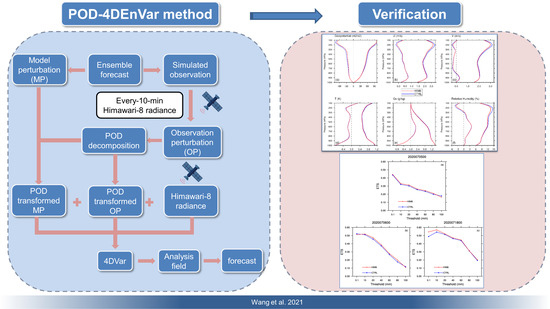
2.1. POD-4DEnVar Algorithm

The POD-4DEnVar method originates from the traditional 4DVar methodology. The cost function of the 4DVar is as follows:

$$J(x)=\frac{1}{2}{(x-x_b)}^{{\rm T}}{B}^{-1}(x-x_b)+\frac{1}{2}{\displaystyle \sum _{k=0}^{s-1}{\left[y_k^{obs}-{\mathit{H}}_k({\mathit{M}}_{t_0\to t_k}(\mathbf{x}))\right]}^{{\rm T}}{R}_k^{-1}\left[{\mathbf{y}}_k^{obs}-{\mathit{H}}_k({\mathit{M}}_{t_0\to t_k}(\mathbf{x}))\right]}$$

(1)

where $\mathbf{x}$ and ${\mathbf{x}}_b$ represent the analysis and background field, respectively; B and R are the error covariances of background and observations, respectively. s is the total number of observations in the assimilation window. ${\mathbf{y}}_k^{obs}$ represents the observations at the analysis time k, ${\mathit{H}}_k$ is the observation operator and ${\mathit{M}}_{t_0\to t_k}$ is the integration of the forecast model from time t₀ to t_k.

$$x_{t_k}={\mathit{M}}_{t_0\to t_k}(x_{t_0})$$

(2)

The incremental format of the 4DVar cost function is as follows:

$$J(x^{\prime })=\frac{1}{2}{(x^{\prime })}^T{B}^{-1}(x^{\prime })+\frac{1}{2}{\displaystyle \sum _{k=0}^{s-1}{\left[y_k^{\prime }(x^{\prime })-(y_k^{obs}{)}^{\prime }\right]}^T{R}_k^{-1}\left[y_k^{\prime }(x^{\prime })-(y_k^{obs}{)}^{\prime }\right]}$$

(3)

where, $x^{\prime }=x-x_b$ represents the analysis increments; $y_k^{\prime }(x^{\prime })$ and ${(y_k^{obs})}^{\prime }$ are the observation increment and observation innovation at analysis time k, respectively. The POD-4DEnVar method applies the POD technique to an ensemble sample, so the background error covariance can also be estimated by ensemble forecasts. Firstly, N ensemble members $(x_1,x_2,\dots ,x_N)$ are obtained by ensemble forecast at time k, which generate N ensemble perturbations $(x_1^{\prime },x_2^{\prime },\dots ,x_N^{\prime })$ to the background field $x_b$. The ensemble perturbations $x_i{}^{\prime }=x_i-x_b$ (i = 1, 2, …, N) make up the model perturbations (MPs) matrix $X_p$. In the meantime, N observation perturbations $(y_1^{\prime },y_2^{\prime },\dots ,y_N^{\prime })$ are constructed by the observation operator $H_k$, constructing the observation perturbation (OPs) matrix $Y_p$.

Since the dimension of the observed variable space is much smaller than that of the model space [23], the POD decomposition is performed on the observation perturbation matrix $Y_p$.

$${(Y^p)}^T(Y^p)=V{\Lambda }^2{V}^{\mathrm{T}}$$

(4)

where $V$ and $\Lambda$ are the decomposed eigenvector and eigenvalue, respectively. The OPs matrix $Y_p$ and MPs matrix $X_p$ are transformed as follows:

$$P_y=Y^{p}V$$

(5)

$$P_x=X^{p}V,$$

(6)

As a result, the POD transformed OPs and MPs are orthogonal and thus independent. At the same time, the error covariances of background B can be represented by the transformed MPs

$$B=P_x{P}_x{}^T/(N-1),$$

(7)

The optimal solutions x’ and y’ can be expressed by the linear combinations of the POD-transformed MPs and OPs, where $\mathsf{\beta }$ represents a set of coefficient vectors:

$${\mathbf{x}}^{\prime }={\mathbf{P}}_x\mathsf{\beta },$$

(8)

$$y^{\prime }={\mathbf{P}}_y\mathsf{\beta },$$

(9)

Thus, substituting (7)-(9) into the incremental format of 4DVar (3), the control variable x’ is replaced by $\mathsf{\beta }$:

$$J(\mathsf{\beta })=\frac{1}{2}(N-1)\cdot {\mathsf{\beta }}^T{P}_x^T{\left(P_x^T\right)}^{-1}{\left(P_x\right)}^{-1}{P}_x\mathsf{\beta }+\frac{1}{2}{\left(P_y\mathsf{\beta }-(y_{}^{obs}{)}^{\prime }\right)}^T{R}^{-1}\left(P_y\mathsf{\beta }-(y_{}^{obs}{)}^{\prime }\right),$$

(10)

After solving the optimal problem of (10) and substituting $\mathsf{\beta }$ in (8), the optimal solution x’ can be simplified into the following form, in which I is the identity matrix.

$$x^{\prime }=P_x{\left[(N-1)I+P_y^T{R}^{-1}{P}_y\right]}^{-1}{P}_y^T{R}^{-1}(y^{obs}{)}^{\prime },$$

(11)

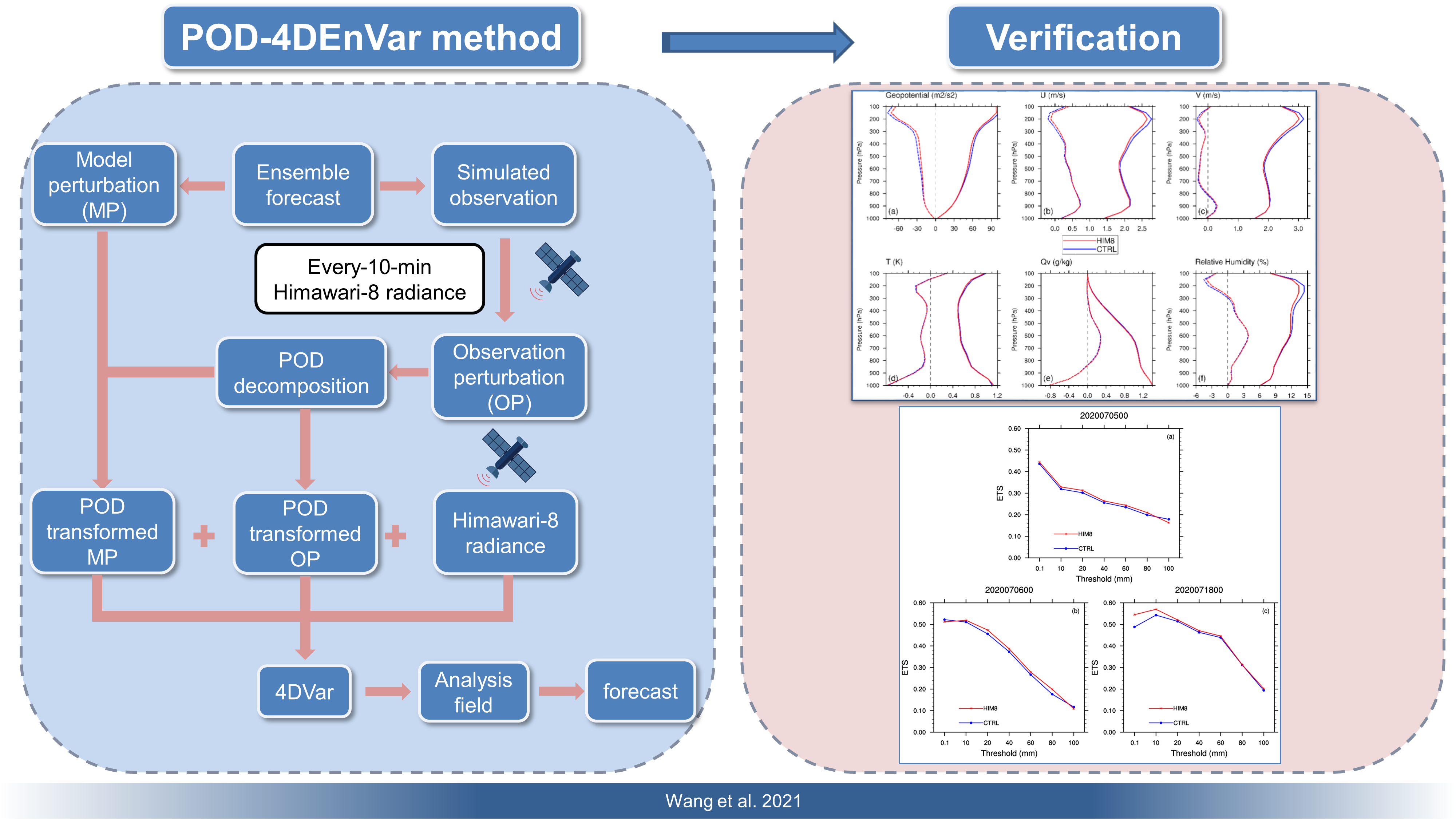
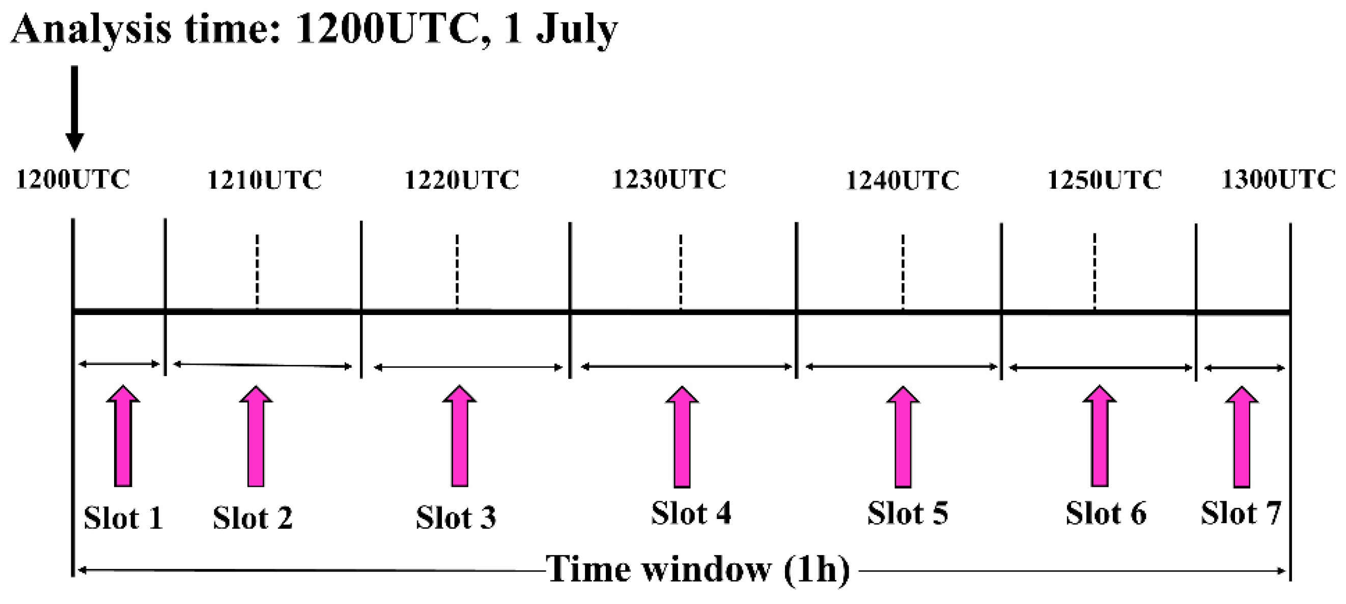
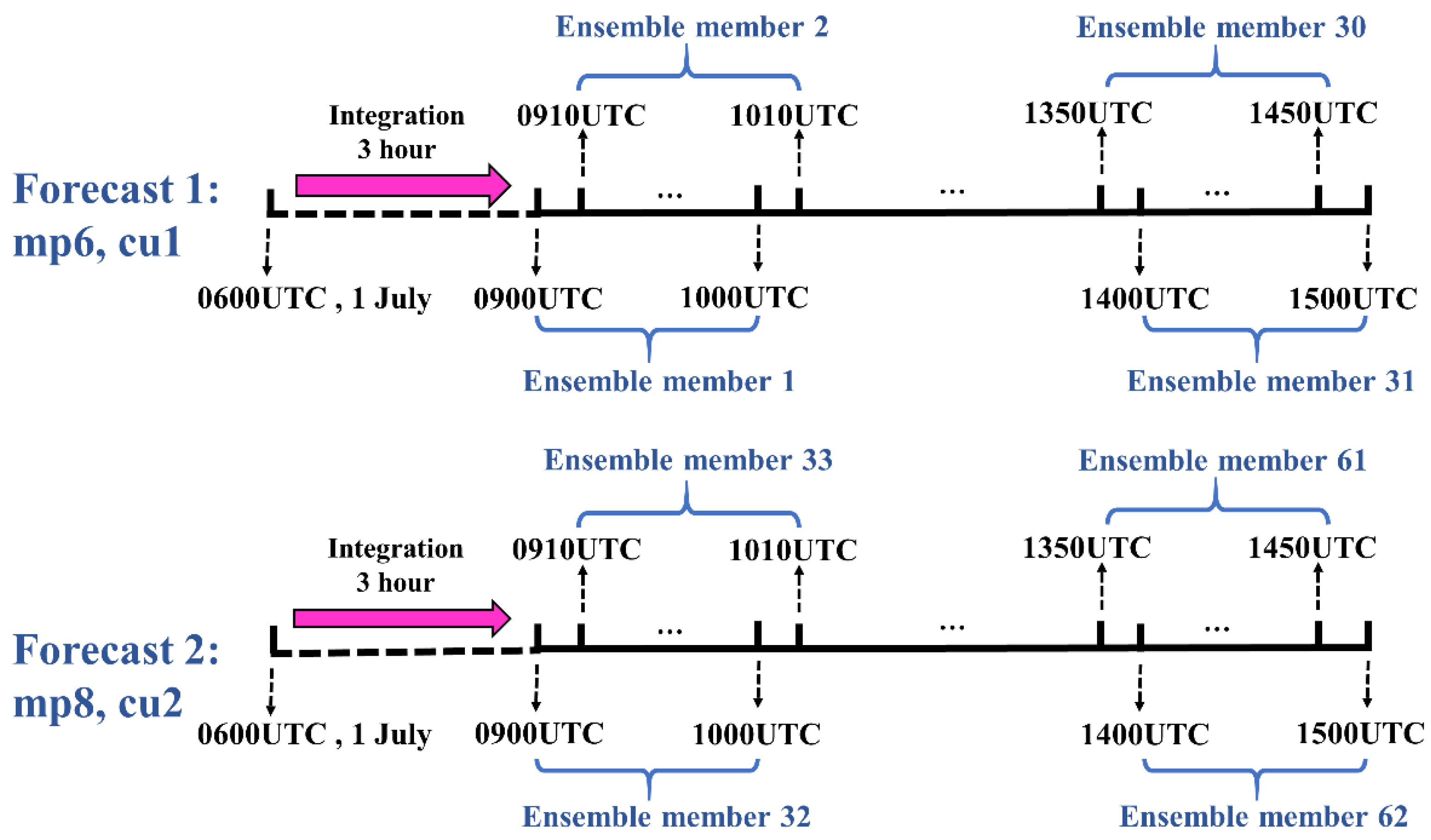
2.2. Four-Dimensional Ensemble Sample Construction

As is shown in the algorithm of the POD-4DEnVar method, the final optimal solution is represented by the POD-transformed model perturbation and observation perturbation matrix. Thus, the construction of ensemble samples plays an important role in the assimilation process. Theoretically, the ensemble size should be sufficiently large to represent the real uncertainty of the atmosphere. However, considering the computational cost and efficiency, limited ensembles have been widely used in assimilation [51]. Historical forecasts can well represent the uncertainty in forecast models with low computational cost [23]. Furthermore, the development of weather systems is directly related with physical processes. Thus, numerical simulations are extremely sensitive to the parameterization schemes in numerical models [52,53,54,55]. In this study, historical forecasts and physical ensembles are combined to construct the four-dimensional ensemble samples.

Since the real every-10-min Himawari-8 radiance is assimilated, the assimilation window was set to 1 h, with the analysis time at the beginning in the assimilation window. Himawari-8 makes 7 observations every 10 min within 1 h, so the assimilation window was divided into 7 sub-windows (slot 1 to 7). Figure 1 shows an example of the assimilation window at 1200 UTC, 1 July 2020. The central times of the 7 sub-windows are 1200, 1210, 1220, 1230, 1240, 1250 and 1300 UTC. The process of four-dimensional ensemble construction is shown in Figure 2. In order to combine a physical ensemble with historical forecasts, two integrations were made from the same initial time, but with different microphysics and cumulus parameterization schemes. First, using the Kessler scheme (microphysics, hereafter “mp6” as it is the 6th parameterization scheme in the WRF model) and the Kain–Fritsch scheme (cumulus parameterization, hereafter “cu1”), a 3-h integration was made from 0600 to 0900 UTC. Then, the output at 0900 UTC was used as the initial condition to make a 6-h integration to 1500 UTC, during which the model output interval was set to 10 min according to Himawari-8 observations. Here, a 4D sliding sampling strategy was applied into the model output. According to the assimilation window, every 7 results made up a sample, corresponding to 7 sub-windows. For example, ensemble 1 was (0900, 0910, 0920, 0930, 0940, 0950, 1000 UTC). Thus, 31 ensemble samples were obtained through the first integration. In the meantime, the same procedure was carried out but with the New Thompson scheme (microphysics, hereafter “mp8”) and the Betts–Miller–Janjic scheme (cumulus parameterization, hereafter “cu2”). Therefore, a total of 62 ensemble members were formed.

2.3. Himawari-8 Observations Quality Control

Himawari-8 was successfully launched by the Japan Meteorological Agency (JMA) on 7 October 2014 and settled in geostationary orbit on 15 October 2015. It is located at 140.7°E, covering the area from 80°E to 160°W and 60°N to 60°S. The Advanced Himawari Imager (AHI) onboard Himawari-8 is comparable to the Advanced Baseline Imager (ABI) onboard GOES-R. The AHI has high spatial resolution, with the highest resolution of 0.5 km and others of 1, 2 and 5 km. The AHI provides scans of the Full Disk (every 10 min), Japan Area (every 2.5 min), Target Area (every 2.5 min), and two Landmark Areas (every 30 s). The AHI has 16 observation bands, of which 3 are visible, 3 are near-infrared and 10 are infrared. Among the 16 bands, 8–10 are water vapor absorption bands (with wavelengths of 6.2, 6.9 and 7.3 µm), which are sensitive to middle-to-upper tropospheric humidity [43]. Thus, bands 8-10 from Himawari-8 are assimilated in this study.

Quality control is the key element in satellite radiance assimilation in order to reduce the random error and systematic bias of radiance. The quality control procedures of AHI observations are as follows [46]: (1) gross check: removing those observations with a brightness temperature higher than 550 K or lower than 50 K; (2) mixture surface type check: rejecting all channels over mixture surface type; (3) cloud liquid water check path check: rejecting those with cloud liquid water check path ≥0.2 kg/m²; (4) relative departure check: removing observations whose bias-corrected innovation exceeds 3 times the observation error standard deviation; (5) absolute departure check: rejecting those whose bias-corrected innovation exceeds 8 K. In addition, only clear-sky radiance is assimilated in this study; thus, cloud detection was required to discard cloud-affected pixels. The AHI level 2 cloud product was used to carry out cloud detection [56]. All the observations were classified into 11 types according to the cloud type, namely clear, cirrus (Ci), cirrostratus (Cs), deep convection, altocumulus (Ac), altostratus (As), nimbostratus (Ns), cumulus (Cu), stratocumulus (Sc), stratus (St) and others. Here, only “clear” observations were assimilated.

Figure 3 presents the spatial distribution of observations and observations minus simulations before and after quality control of AHI channel 9 at 0000 UTC 20 July 2020. The simulated brightness temperature was calculated using Community Radiative Transfer Model (CRTM)-v2.2.3. The coverage of all observations before quality control is shown in Figure 3a, which includes both “good” and “bad” data. After quality control, the difference between the observed and simulated brightness temperature from background fields (OMB) is shown in Figure 3b. It can be seen that not all the observations pass the quality control, with “bad” data (about 65.5%) rejected in this step. However, the differences between background and observations still reach up to ±4 K, with some OMBs being apparently larger than others. Figure 3c shows the difference between the observed and simulated brightness temperature from analysis fields (OMAs). The OMA is clearly reduced for those with larger OMB values, especially those above 32°N. To correct the systematic bias of radiance observations, the variational bias correction (VarBC) embedded in the WRFDA was applied in the POD-4DEnVar assimilation [57]. Figure 4 shows the scatter plots of the observations (OBS) and simulated brightness temperature from background (BAK) and analysis (ANA) fields. Figure 4a,b compares the scatter plots when bias correction (BC) is carried out or not. Apparently, after the bias correction, the mean bias clearly reduced from 0.961 to 0.061 (by almost 93%), and the root mean square error (RMSE) reduced from 1.589 to 1.268 (by almost 20%). In comparison, ANA was in better agreement with OBS, with a reduction in mean bias to 0.051 (by almost 16%), in standard deviation (STDV) to 0.832 (by almost 34%) and in RMSE to 0.833 (by almost 34%). The results indicate that quality control and bias correction are effective when assimilating Himawari-8 radiance.

3. Experiment Design

This study employed the WRF-v3.9.1.1 model [58] to make ensemble forecasts and deterministic forecasts. The WRF model is configured with a two-nested domain, as shown in Figure 5. Clearly, the outer domain is in the coverage of Himawari-8 observations mostly, and the inner domain is in full coverage of observations. The horizontal resolution of the outer domain is 15 km, with 281 × 281 model grid points. The inner domain is of 5-km horizontal grid spacing, with 322 × 298 model grid points mainly covering seven provinces of China. Both domains are configured with the model top of 50 hPa and 35 vertical levels. The main physical parameterization schemes used in the WRF model are listed in

Table 1. Parameterization schemes.

Physics	Schemes
Microphysics	Ensembles 1-31: Kessler scheme Ensembles 32-62: New Thompson scheme
Cumulus parameterization (not used in inner domain)	Ensembles 1-31: Kain–Fritsch scheme Ensembles 32-62: Betts–Miller–Janjic scheme
Planetary boundary layer	Yonsei University scheme
Surface layer	Revised MM5 Monin–Obukhov scheme
Longwave radiation	RRTM scheme
Shortwave radiation	Dudhia scheme

.

In order to investigate the impacts of assimilating Himawari-8 radiance, two parallel experiments were designed, denoted as CTRL and HIM8. The CTRL experiment assimilated conventional observations in the inner domain [59], including radiosonde, synoptic observations, ships, airport reports, etc. The HIM8 experiment assimilated all the observations in CTRL plus every-10-min clear-sky radiance from Himawari-8 AHI channels 8, 9 and 10 in the inner domain. All the observations were thinned to 30 km in order to reduce the correlations [44,45,46]. The CRTM was used as the observation operator [60,61]. The WRF model utilizes National Centers for Environmental Prediction (NCEP) Final (FNL) Operational Model Global Tropospheric Analyses as the initial and lateral condition.

To evaluate the results statistically, a one-month analysis and forecast were conducted from 1 July to 31 July 2020. Figure 6 shows the schematic of the analysis and forecast configuration. Assimilation was performed at 0000 UTC each day. The assimilation window was set to 1 h, with the analysis time at the beginning of the window. As mentioned above, the window was divided into seven sub-windows, corresponding to seven observations in an hour; Figure 6 shows an example from 0000 UTC 15 July. Ensemble forecasts were carried out before assimilation to provide ensemble samples. Furthermore, 24-h forecasts were made at 0000 UTC each day to evaluate the quality of forecasts. The evaluation was based on the average results, which is more valid statistically than just one single analysis and forecast.

4. Results and Discussion

4.1. RMSE Verification against ERA-5 Data

In order to evaluate the impacts of assimilating Himawari-8 radiance, the fifth generation of the European Center for Medium Range Weather Forecasts (ECMWF) reanalysis (ERA-5) data was used as the “truth” [42,44,62,63,64].

Figure 7 displays the vertical profiles of average bias (dashed lines) and RMSE for geopotential, horizontal wind, temperature, water vapor mixing ratio and relative humidity from the analysis fields. The blue and red lines represent the CTRL and HIM8 experiments against ERA5, respectively. For geopotential (Figure 7a), the bias between CTRL and HIM8 is close under 850 hPa. HIM8 yields relatively lower bias from 850 hPa to the top. The results of RMSE are similar to those of bias. The RMSE of HIM8 is clearly reduced above 850 hPa. For the U component of horizontal wind (Figure 7b), lower bias is found in HIM8 at upper levels. However, the RMSE is clearly improved from almost 900 hPa to the top. Compared to U, the improvement of the V component is much clearer (Figure 7c) when assimilating radiance. Lower bias in HIM8 was found, except at levels under 800 hPa. Especially for RMSE, an overall improvement in HIM8 was found from 900 hPa. For temperature (Figure 7d), small but positive impacts were found in HIM8 compared to the CTRL experiment, especially in middle and lower levels of RMSE. For the water vapor mixing ratio (Figure 7e), the impact of assimilation is smaller in the analysis field, and bias and RMSE are reduced in the middle and upper levels. However, the assimilation of Himawari-8 radiance has noticeable impacts on the relative humidity (Figure 7f). HIM8 shows little reduction in bias and RMSE in the middle and lower levels. The difference between the two experiments becomes clear above 500 hPa. It demonstrates that the relative humidity field of HIM8 is more favorable to ERA-5 data in the upper levels. In order to quantitively determine the difference between CTRL and HIM8,

Table 2. The geopotential analysis average bias and RMSE values at different heights.

	Pressure (hPa)	1000	950	900	850	800	700	600	500	400	300	200	100
Bias	CRTL	−2.151	−10.83	−16.43	−19.07	−20.32	−21.98	−24.60	−27.64	−30.51	−36.18	−65.74	−69.98
	HIM8	−2.198	−10.87	−16.26	−18.57	−19.48	−20.41	−22.23	−24.21	−26.24	−31.96	−60.59	−64.28
	Improvement (%)	−2.14	−0.35	1.02	2.61	4.16	7.13	9.65	12.39	14.00	11.67	7.83	8.16
RMSE	CRTL	2.864	16.32	26.34	33.16	38.48	46.91	53.43	57.86	61.76	69.36	92.69	103.8
	HIM8	2.914	16.38	26.22	32.79	37.83	45.59	51.31	54.94	58.66	66.75	88.53	97.79
	Improvement (%)	−1.74	−0.33	0.45	1.13	1.69	2.81	3.97	5.06	5.01	3.76	4.49	5.84

displays the specific bias and RMSE values at different vertical levels of geopotential as an example. Statistically, the average improvement in bias is 6.44%, with the largest improvement of 14.0% at 400 hPa. The average improvement in RMSE is 2.69%, with the largest improvement of 5.84% at 100 hPa.

Figure 8 displays the vertical profiles of average bias and RMSE from 24-h forecasts. The improvement of geopotential (Figure 8a) is much clearer when a 24-h forecast is conducted. The bias decreased from 700 to 100 hPa in HIM8. The same improvement can also be found in RMSE, which decreased from 800 to 100 hPa. A relatively slight reduction was found for the U and V components of wind (Figure 8b,c). The bias from CTRL and HIM8 was close for U and V, with little improvement in the middle levels. Positive impacts were found in RMSE for U and V. The RMSE in HIM8 is reduced from 900 to almost 100 hPa for U, and the reduction is much more apparent than V. For temperature (Figure 8d), lower bias appears between 800 and 600 hPa in HIM8 compared to CTRL. A similar reduction was found in RMSE, with lower RMSE in the middle and lower levels. The impact of assimilation on water vapor mixing ratio forecast (Figure 8e) is slight and mainly in the middle levels. For relative humidity (Figure 8f), the difference between the two experiments is not as clear as in the analysis field. The main improvements were found between 800 and 600 hPa. The specific bias and RMSE values of 24-h geopotential forecasts are taken as an example to be analyzed quantitatively in

Table 3. The geopotential 24-h forecast average bias and RMSE values at different heights.

	Pressure (hPa)	1000	950	900	850	800	700	600	500	400	300	200	100
Bias	CRTL	−2.589	−1.662	2.733	6.759	6.765	−7.836	−14.138	−16.09	−11.04	−6.797	−19.67	−36.02
	HIM8	−2.554	−1.169	4.118	9.224	10.14	−3.353	−9.498	−11.57	−6.490	−2.126	−15.68	−30.50
	Improvement (%)	1.36	29.65	−50.64	−36.45	−49.93	57.20	32.82	28.07	41.26	68.71	20.29	15.34
RMSE	CRTL	2.967	14.20	25.98	36.38	44.44	59.85	73.97	82.83	84.51	87.76	99.80	82.58
	HIM8	2.913	14.06	25.82	36.06	43.68	57.18	68.93	77.27	78.57	81.87	93.81	77.09
	Improvement (%)	1.84	0.94	0.59	0.87	1.72	4.46	6.81	6.72	7.03	6.71	6.00	6.65

. Compared to CTRL, the average of forecast bias is reduced by 7.57%, with the largest reduction of 68.71% at 300 hPa. Meanwhile, the average forecast RMSE is reduced by 4.23%, with the largest reduction by 7.03% at 400 hPa. Overall, Himawari-8 radiance assimilation with the POD-4DEnVar method shows a positive impact on the main meteorological elements’ analysis and forecasts.

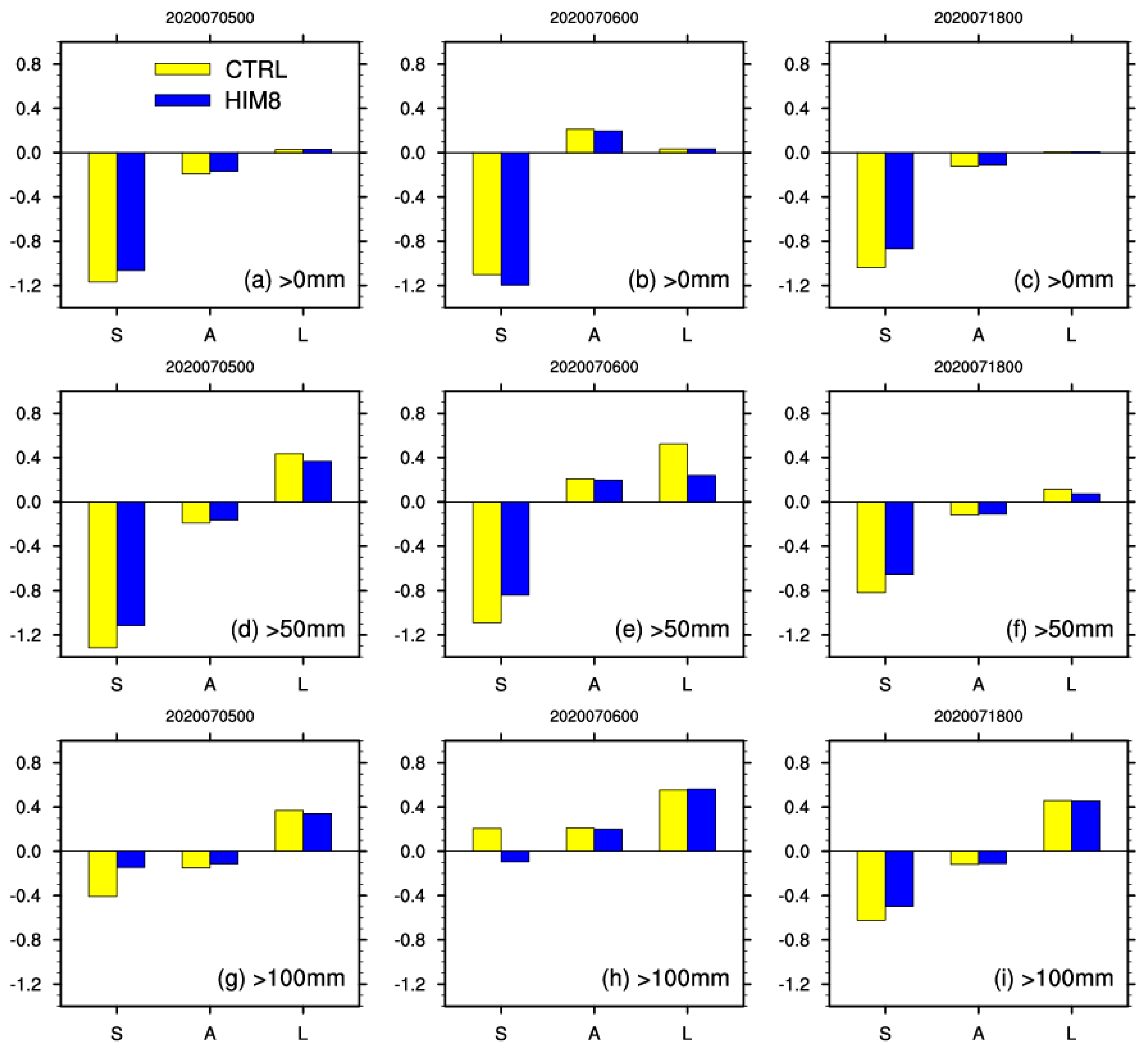
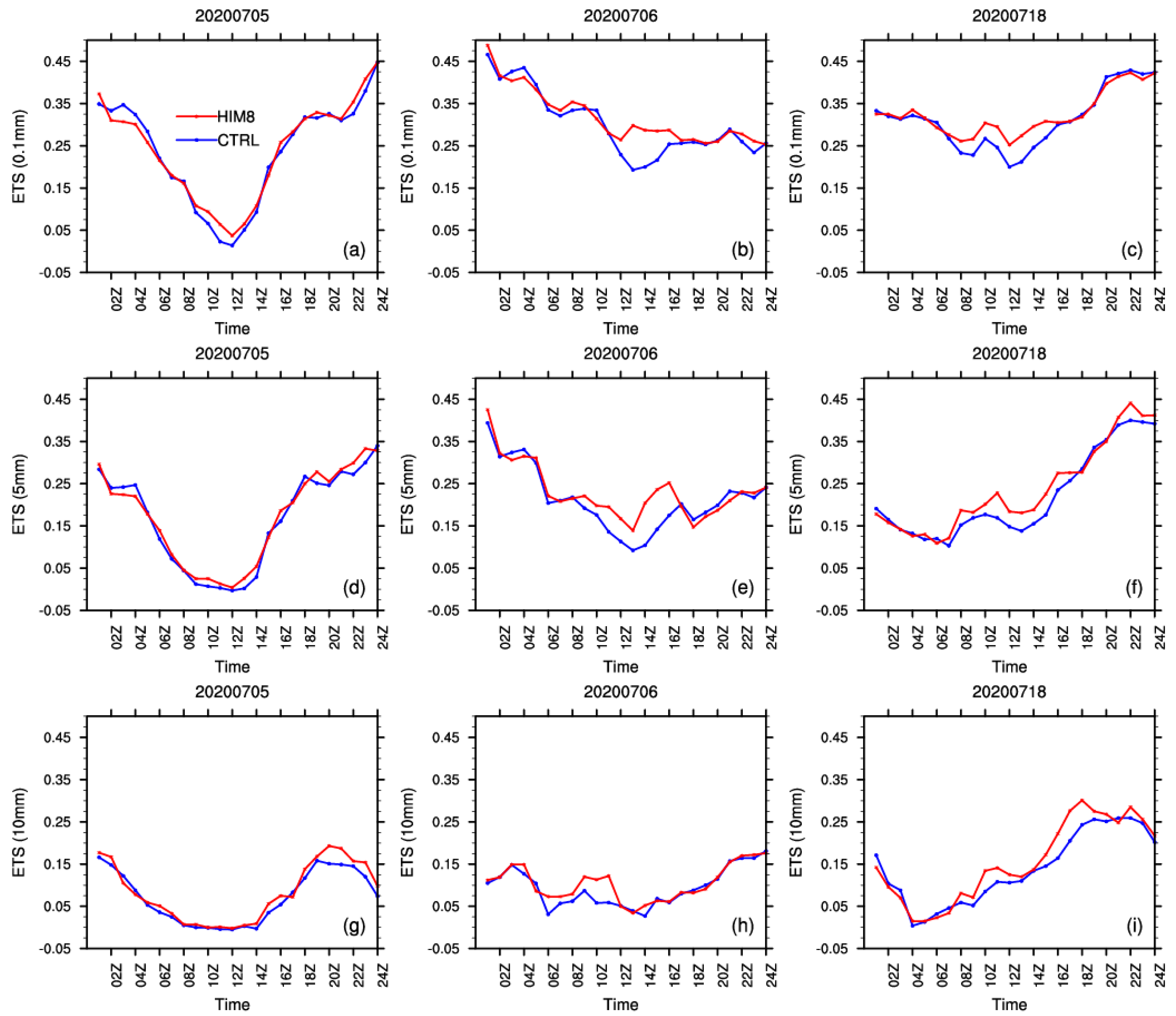
4.2. Impacts on Rainfall Forecasts

Rainfall events usually have a great influence on people’s daily life, even causing meteorological disasters. Thus, it is important that rainfall should be skillfully predicted by the numerical model. Thus, rainfall forecasting was used to further evaluate the performance of Himawari-8 radiance assimilation with the POD-4DEnVar method. The China Hourly Ground Station Precipitation merged with the Climate Prediction Center morphing precipitation products (CMORPH) was used for evaluation. During the one-month experiments, three concentrated precipitation events in the inner domain were found, taking place on 5 July 6 July and 18 July 2020. The domain-averaged precipitation amount and its every-3-h growth are displayed in Figure 9. On 5 July (Figure 9a), the domain-averaged precipitation amount decreased until 1200 UTC, with a rapid decrease from 0400 to 0600 UTC. After 1200 UTC, the rainfall began to strengthen, especially at 2000 UTC when a quick intensification of rainfall was found. On 6 July (Figure 9b), there were two periods of negative 3-h growth from 0400 to 0700 UTC and from 1100 to 1900 UTC. The precipitation weakened quickly after 1200 UTC, reaching the weakest intensity at 1800 UTC. After that, the rainfall rapidly strengthened. On 18 July (Figure 9c), the precipitation was continuously strengthening after 0500 UTC. The largest increases were found at 1000 and 1800 UTC. After 2200 UTC, the amount of precipitation decreased slightly.

Figure 10 shows the equitable threat score (ETS) of different thresholds for 24-h accumulated precipitation from 0000 to 2400 UTC. The ETS ranges between –1/3 and 1, with negative or zero values indicating no skill and 1 indicating a perfect score [65]. It is seen that the ETS values generally decrease as the precipitation strengthens, indicating that the prediction skill of weaker rainfall is better than that of heavier rainfall, no matter for CTRL or HIM8. On 5 July (Figure 10a), positive impacts were found in HIM8 compared to CTRL, except for the 100 mm threshold. On average, the ETS of HIM8 increased by 1.74% compared to CTRL. On 6 July (Figure 10b), the ETS of HIM8 increased compared to CTRL, except for the 0.1 and 100 mm thresholds. The ETS of HIM8 relatively improved by 2.58% on average. On 18 July (Figure 10c), HIM8 yielded a higher ETS than CTRL generally, demonstrating that the assimilation of Himawari-8 radiance further enhanced the performance for the rainfall prediction on 18 July. The ETS of HIM8 improved by 3.68% on 18 July. On average, the ETS of 24-h accumulated precipitation improved by 2.67% over the three cases, demonstrating the positive impact of Himawari-8 radiance assimilation on rainfall forecasts.

To objectively and quantitatively verify the precipitation forecast, the Structure, Amplitude and Location (SAL) assessment method was adopted as the second verification method [66]. The A component measures the relative deviation of the domain-averaged quantitative precipitation forecasts. The L component is related to the location of precipitation, such as the displacement of the precipitation field’s center of mass. The S component measures the predicted precipitation objects with observations, such as whether the objects are too large or too small. Perfect predictions are characterized by 0 for the S, A and L components, indicating that smaller absolute values yield better forecasts [66]. Figure 11 displays the SAL results of 24-h accumulated precipitation from the two experiments. On 5 July (Figure 11a,d,f), the S value in HIM8 was clearly closer to zero compared to CTRL, showing better precipitation structure prediction, especially for the 100 mm threshold. All the A values were negative for the three thresholds, indicating that the model underestimates the area-integrated precipitation. However, with radiance assimilation, lower absolute A values were obtained for all the thresholds, showing improvements in the amplitude prediction. For L, both experiments yielded small values for 0 mm, indicating excellent performance in predicting the precipitation location. HIM8 yielded a slightly higher L value for 0 mm and a lower L value for 50 and 100 mm. On 6 July (Figure 11b,e,h), HIM8 showed slightly larger structure errors than CRTL did for 0 mm but a clearly smaller structure error for 100 mm. For amplitude, all the experiments overestimated the 24-h accumulated precipitation, but HIM8 had smaller errors in terms of amplitude. For location, smaller errors were found for HIM8 at 0 and 50 mm. With the 100 mm threshold, HIM8 slightly overestimated the location more than CTRL did. For 18 July (Figure 11c,f,i), the structure of rainfall was better predicted in HIM8 for all thresholds. For amplitude, both experiments underestimated the precipitation intensity, with HIM8 showing smaller errors for all the thresholds. For location, similar to the results on 5 July the L values from both experiments for 0 mm were almost zero, indicating that the rainfall location was nearly perfectly predicted in both experiments. At the 50 mm threshold, the location error was clearly reduced in HIM8 compared to CTRL. The location errors of the two experiments were close at 100 mm, showing little impact of radiance assimilation on location prediction. Overall, the SAL evaluation indicates that assimilating Himawari-8 radiance can improve the rainfall prediction from different aspects.

From the verification scores above, overall positive effects were found with the Himawari-8 radiance assimilation. To further investigate the impacts, Figure 12 presents the spatial distribution of 24-h accumulated precipitation from observations (OBS) and the two experiments (CTRL and HIM8), initialized at 0000 UTC on 5 July 6 July and 18 July. On 5 July, the observed rainfall (Figure 12a) was mainly distributed from west to east across Hubei Province, Anhui Province and Jiangsu Province. Heavy rainfall occurred in Hubei Province. The precipitation patterns in both CRTL (Figure 12d) and HIM8 (Figure 12g) are separated into two areas. Both experiments overestimated the precipitation in north Hunan and south Anhui but underestimated the precipitation in south Hubei. However, compared with CTRL, HIM8 simulated relatively weaker rainfall in south Anhui and Hubei, which reduced forecast errors against the observations. On 6 July the observed precipitation pattern (Figure 12b) moved to the east. The simulated rainfall area of CRTL (Figure 12e) slightly smaller than the observations, whereas HIM8 agreed more with the observations. Both experiments overestimated the intensity of heavy rainfall, especially for heavier rainfall (>100 mm). There was clear heavy rainfall in the northwest of Zhejiang Province according to CTRL, which was not found in observations. However, HIM8 corrected the overestimation in Zhejiang Province with radiance assimilation. On 18 July the area of precipitation became clearly larger than that on the first two days, covering most of the domain in the middle and north. Heavy rainfall occurred in Anhui Province. The CTRL and HIM8 experiments (Figure 12f,i) both clearly underestimated the heavy rainfall in Anhui Province. In Hunan Province, both experiments overestimated the precipitation compared with observations, and HIM8 showed relatively weaker rainfall intensity. Thus, the distribution of precipitation shows that simulated precipitation with radiance assimilation is more favorable with observations on the whole. However, it was also found that after assimilation, there was still some overestimation of precipitation, which should be further improved in the future.

Observations with higher temporal frequency are supposed to improve the prediction of rapidly changing systems, such as rapidly developing rainfall. Figure 13 shows the ETS for hourly accumulated precipitation with thresholds of 0.1, 5 and 10 mm. The hourly ETS was calculated from 0000 to 2400 UTC on 5, 6 and 18 July. For 5 July the ETS results between the two experiments are quite close for the 0.1 mm threshold (Figure 13a), with a slightly higher ETS for HIM8 than for CTRL. For 5 mm (Figure 13d), higher ETS was found in HIM8 between 08Z and 14Z. For 10 mm (Figure 13g), the ETS clearly improved after 14Z in HIM8 compared to CTRL, with the largest improvement at 20Z. As shown in Figure 9a, the precipitation strengthened between 14Z and 20Z. The higher ETS at the 10 mm threshold indicates that HIM8 better predicted the rapid intensification of rainfall on 5 July. For 0.1 mm on 6 July (Figure 13b), the ETS values between the two experiments are close until 12Z, after which the ETS for HIM8 clearly increases hourly. For 5 mm (Figure 13e), HIM8 also clearly increases the ETS of CTRL, especially between 08Z and 17Z. For 10 mm (Figure 13h), the improvement becomes clear from 04Z. As shown in Figure 9b, there was a sharp decrease and increase in the precipitation amount before and after 16Z, showing that rainfall was developing rapidly. The larger hourly ETS of HIM8 during that time demonstrates the advantage of assimilating high temporal resolution observations in rapidly weakening precipitation forecasts. However, when the precipitation sharply strengthened, the performance of the two experiments was similar. For 18 July a higher ETS of HIM8 could be found at 0.1 mm (Figure 13c). HIM8 obtained a higher ETS from 08Z to 15Z. For 5 mm (Figure 13f), the scores of the two experiments seemed to be close before 07Z, even with the lower ETS of HIM8. After 07Z, HIM8 showed an overall higher score until 18Z. For 10 mm (Figure 13i), the clearest improvement for HIM8 occurred between 08Z to 22Z. Figure 9c shows that the rainfall on 18 July was continuously strengthening, with the strongest intensification around 18Z. A higher ETS of HIM8 was found at that time in different thresholds. These results show that the radiance assimilation experiment better predicted the hourly accumulated precipitation.

The average percentages of relative improvement are also displayed in

Table 4. The relative improvement in hourly ETS in HIM8 compared with CTRL.

	5 July	6 July	18 July	Average
0.1 mm	2.09%	5.40%	4.20%	3.90%
5 mm	3.96%	9.0%	7.90%	6.95%
10 mm	15.52%	11.20%	11.40%	12.71%
Average	7.19%	8.53%	7.83%	7.85%

. For different days, the hourly ETS on 5 July improved with assimilation by about 7.19%, with a maximum improvement of 15.52% in the 10 mm threshold. The ETS on 6 July improved by 8.53% on average, with the largest improvement of 11.20% in 10 mm. The relative improvement on 18 July was 7.83%. Comparing the different thresholds, the largest improvement was found in 10 mm. This shows that the prediction for heavy rainfall in a short time with assimilation is better than that without assimilation. From all the cases, the ETS of HIM8 increased by 7.85% compared to CTRL on average. Overall, the assimilation of Himawari-8 radiance with the POD-4DEnVar method has positive impacts on short-term precipitation forecast, especially for rapidly developing precipitation.

4.3. Discussion

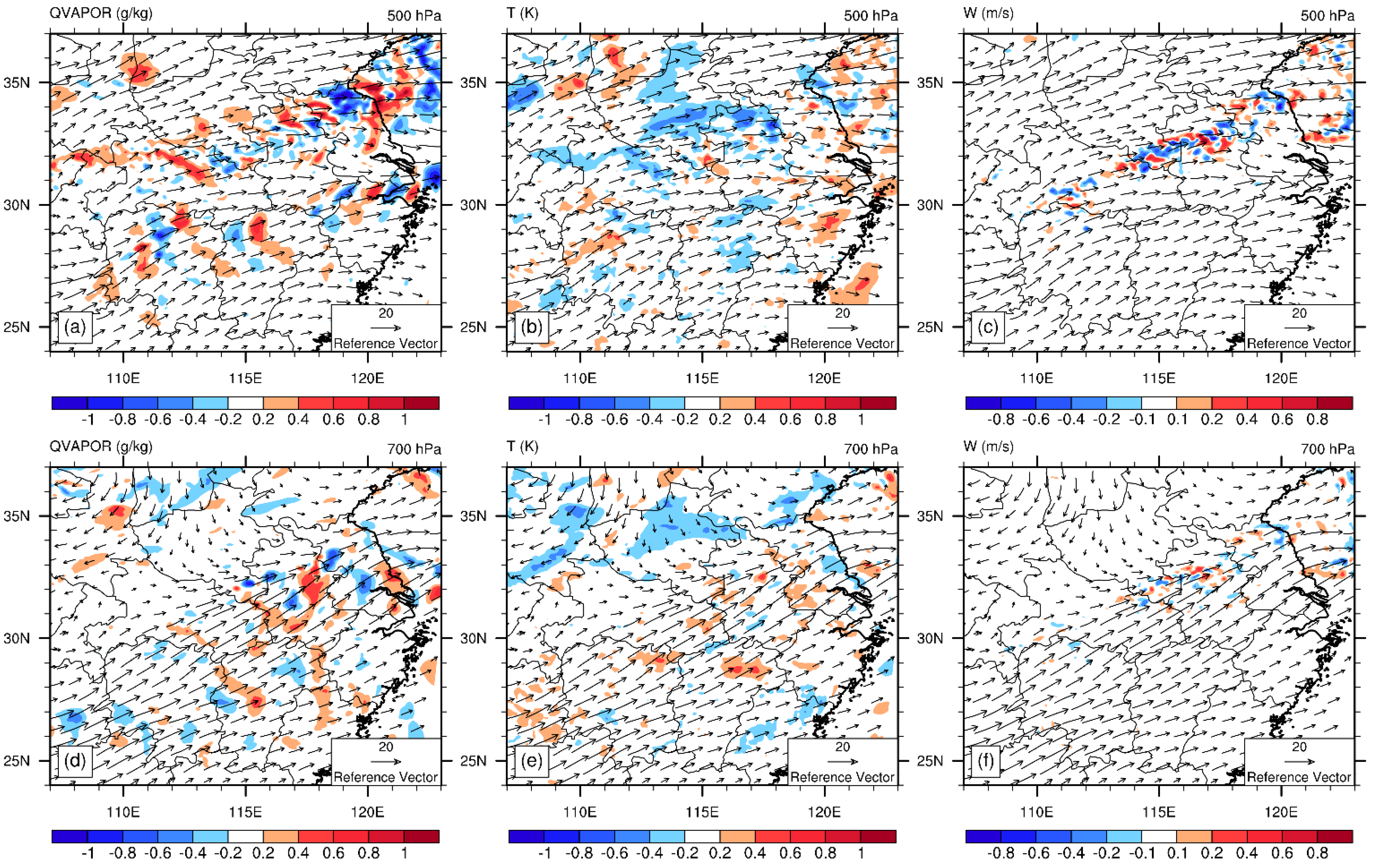
4.3.1. The Initial Increments

As shown in the evaluation results above, assimilating Himawari-8 radiance reduces the average bias and RMSE of meteorological elements’ analyses and forecasts. In addition, assimilation further improves the score skills of quantitative rainfall forecast as well as the structure, amplitude and location forecast. To further investigate the impacts of radiance assimilation, the initial increments are analyzed and discussed in this section. Initial increments show the difference between analysis and background, representing the change from background to analysis by assimilating Himawari-8 radiance.

On 18 July, heavy rainfall appeared in the middle of Anhui Province (31°N–33°N, 114°E–118°E). Figure 14 shows the spatial distribution of the water vapor mixing ratio (QVAPOR), temperature (T) and vertical velocity (W) at different pressure levels at 0000 UTC on 18 July 2020, when rainfall of varying intensity occurred around 30°N (Figure 12). The vectors represent the analysis of horizontal wind field, which provides the circulation patterns. For QVAPOR, the spatial distribution of increments is all over the inner domain, mostly in the precipitation area. The water vapor at 700 hPa was increased in the middle of Anhui after assimilation, with a maximum of almost 0.8 g/kg. At 500 hPa, the increments varied in different areas, with both increases and decreases in water vapor in Anhui. Thus, assimilation of Himawari-8 radiance mainly increases the lower-level water vapor in the heavy rainfall area. More water vapor transport in the lower level is provided for the development of precipitation, helping to strengthen the heavy rainfall in the middle of Anhui Province. The change in temperature after assimilation was slight in the precipitation area, which was dispersed and small, with few cooling effects at 500 hPa and few warming effects at 700 hPa. Thus, assimilating Himawari-8 radiance has little effect on temperature in the precipitation area. However, vertical velocity increments were clearly found in the precipitation area at both 500 and 700 hPa. The positive increments were found in the area where there was clear horizontal wind convergence at 700 hPa. Horizontal wind convergence at the lower level means that there is clear air updraft. Thus, the positive increments indicate that assimilation further strengthens the updraft in the precipitation area, which is beneficial for precipitation development. In addition, the increment at 500 hPa is stronger than that at 700 hPa, demonstrating that Himawari-8 radiance changes the mid-level vertical velocity more than the lower-level one. Overall, the impacts of Himawari-8 radiance on the initial field are mainly found in water vapor and vertical velocity in precipitation areas, which helps improve rainfall prediction.

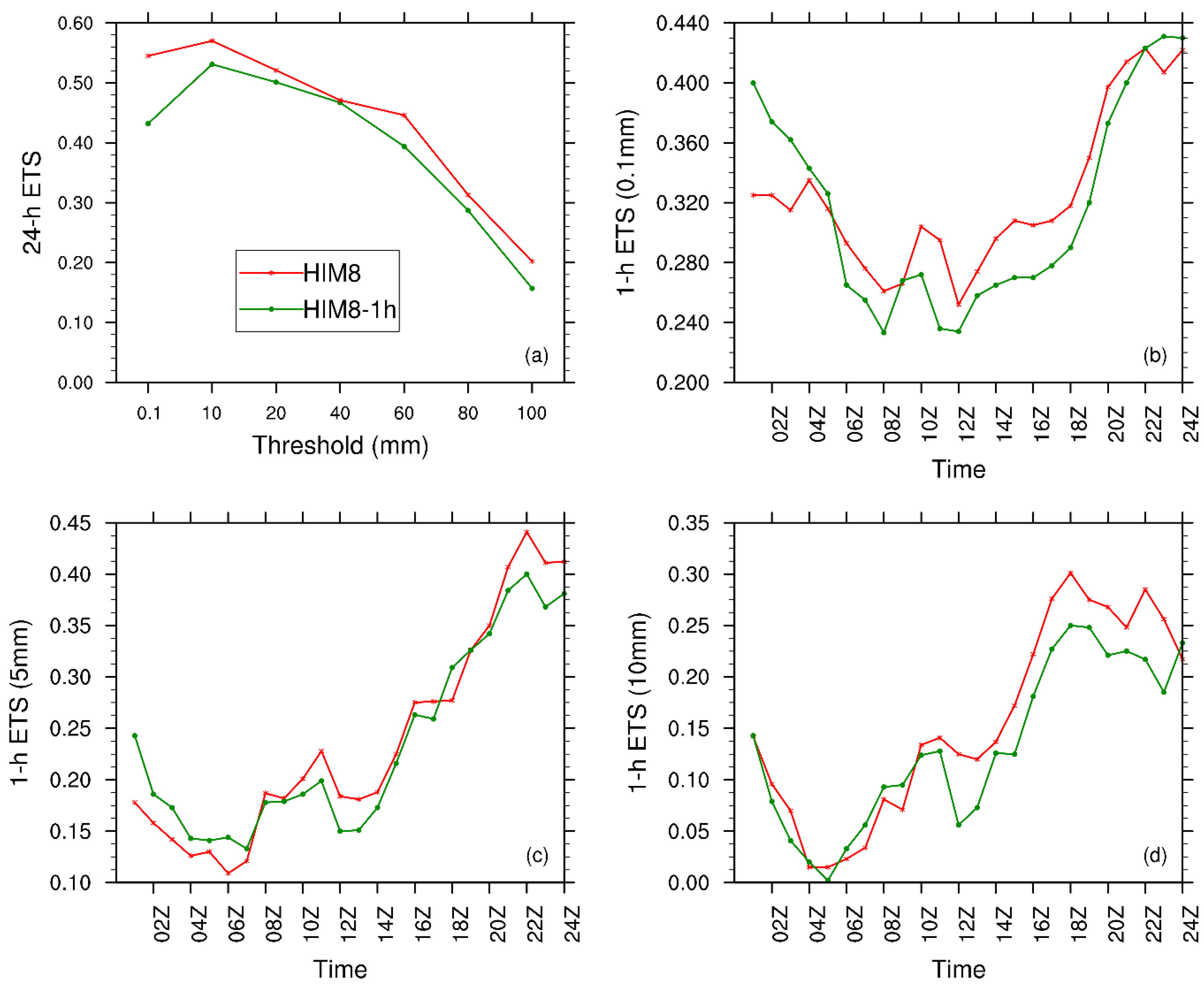
4.3.2. The Effect of Observation Frequency

The hourly precipitation ETS results show that assimilation of every 10-min radiance data with POD-4DEnVar improves the prediction of rapidly changed rainfall events. To investigate the advantages of assimilating high observing frequency radiance data, another assimilation experiment was conducted, HIM8-1h, which assimilates all the observations in CTRL plus every 1-h Himawari-8 radiance. Correspondingly, the assimilation window was set to 6 h, with seven observations made within the assimilation window. An ensemble was made for HIM8-1h with the same method described in Section 2.2, but with a different temporal resolution. The other configurations in assimilation and forecast procedure are the same as HIM8.

Figure 15 shows the ETS results in HIM8 and HIM8-1h on 18 July 2020 as a case study. For 24-h accumulated precipitation (Figure 15a), in general, the ETS for HIM8 was increased compared to HIM8-1h. The increase was much more apparent in the 0.1, 10 and 20 mm thresholds. On average, HIM8 improved the 24-h accumulated precipitation ETS by 12.75% compared to HIM8-1h, with the greatest improvement of 28.66% in 100 mm precipitation. As the results in Section 4.2 demonstrate the positive impacts of assimilation on the rapidly developed rainfall, the same evaluation was carried out on the hourly evolution of precipitation. Figure 15b–d display the hourly accumulated precipitation ETS for different thresholds on 18 July. For 0.1 mm (Figure 15b), the ETS of HIM8 improved between 05Z and 21Z. Clear improvements were found when the precipitation was continuously strengthening. The same results appeared at larger thresholds, where, in the first few hours, HIM8-1h presented better ETS results than HIM8. However, as the precipitation developed, assimilating every-10-min radiance yielded clearly higher ETS results than HIM8-1h. Averaging the different thresholds, the hourly accumulated precipitation ETS improved by 15.88% in HIM8 compared to HIM8-1h. The largest increases in ETS were found at 15Z for 0.1 mm, 12Z for 5 mm and 12Z for 10 mm thresholds. As shown in Figure 9, the precipitation on 18 July continuously strengthened at 08Z and 18Z. Thus, the advantage of assimilating high observational frequency data is revealed when the precipitation is rapidly strengthening.

4.3.3. The Effect of the Assimilation Method

To quantitatively discuss the advantage of assimilating Himawari-8 radiance data with the POD-4DEnVar method, it was compared with the traditional 3DVar assimilation method [59]. The analysis time of 3DVar was set to 0000 UTC on 18 July with the background field provided by a 6-h forecast using the WRF model. The assimilation window was ±3 h, with the analysis time at the center of the window. The other configurations were the same as in the POD-4DEnVar experiments. A comparison of precipitation forecasts was completed.

Table 5. The ETS values of 24-h accumulated precipitation for different thresholds.

	0.1 mm	10 mm	20 mm	40 mm	60 mm	80 mm	100 mm
POD-4DEnVar	0.545	0.57	0.521	0.471	0.446	0.313	0.202
3DVar	0.487	0.453	0.471	0.442	0.385	0.289	0.194

and

Table 6. The ETS values of hourly accumulated precipitation for different thresholds.

	0.1 mm		5 mm		10 mm
	POD-4DEnVar	3DVar	POD-4DEnVar	3DVar	POD-4DEnVar	3DVar
01Z	0.325	0.294	0.178	0.177	0.142	0.148
02Z	0.325	0.323	0.158	0.19	0.096	0.103
03Z	0.315	0.334	0.142	0.18	0.07	0.103
04Z	0.335	0.353	0.126	0.179	0.015	0.092
05Z	0.316	0.331	0.13	0.165	0.015	0.067
06Z	0.293	0.286	0.109	0.136	0.023	0.052
07Z	0.276	0.256	0.121	0.125	0.034	0.072
08Z	0.261	0.234	0.187	0.143	0.081	0.042
09Z	0.266	0.213	0.182	0.161	0.071	0.064
10Z	0.304	0.233	0.201	0.167	0.134	0.08
11Z	0.295	0.224	0.228	0.159	0.141	0.096
12Z	0.252	0.202	0.184	0.117	0.125	0.072
13Z	0.274	0.218	0.181	0.133	0.12	0.08
14Z	0.296	0.245	0.188	0.175	0.137	0.118
15Z	0.308	0.277	0.225	0.224	0.172	0.123
16Z	0.305	0.284	0.275	0.262	0.222	0.165
17Z	0.308	0.285	0.276	0.266	0.276	0.209
18Z	0.318	0.277	0.277	0.258	0.301	0.216
19Z	0.35	0.301	0.326	0.282	0.275	0.235
20Z	0.397	0.333	0.35	0.304	0.268	0.216
21Z	0.414	0.345	0.407	0.319	0.248	0.205
22Z	0.423	0.386	0.441	0.352	0.285	0.255
23Z	0.407	0.396	0.411	0.364	0.256	0.226
24Z	0.422	0.409	0.412	0.41	0.217	0.188

display the ETS values of 24-h and hourly accumulated precipitation with different assimilation methods. On average, assimilation with the POD-4DEnVar method improved the 24-h accumulated precipitation by 11.88% (Table 5) compared to assimilation with the 3Dvar method. The hourly accumulated precipitation ETS was also evaluated between the two assimilation methods. The results show that the POD-4DEnVar method improved the hourly ETS by 11% on average (Table 6). Overall, the quantitative results indicate that assimilating Himawari-8 radiance data with the POD-4DEnVar method outperforms the traditional 3DVar method.

5. Conclusions

In this study, the potential impacts of assimilating every-10-min Himawari-8 radiance data were investigated based on a four-dimensional ensemble variation assimilation method. To assimilate Himawari-8 AHI radiance data, quality control, especially cloud detection, was first conducted. Based on the POD-4DEnVar method, the assimilation window was designed according to the frequency of Himawari-8 observations used in this study. In addition, historical forecasts and physical ensembles were combined in order to make ensembles as well as reduce computational costs. The results suggest that the simulated radiance after quality control and bias correction procedures agrees more with observations, indicating that radiance with “good” quality is guaranteed in the assimilation system.

The impacts of Himawari-8 radiance assimilation on the analysis and forecast of the main meteorological elements were examined. Clear positive effects were found for geopotential, wind field and relative humidity. The impacts on temperature and water vapor mixing ratio were small but still positive overall. An evaluation of rainfall prediction was also conducted to further examine the impacts of assimilation. On average, the HIM8 experiment improved the ETS of 24-h accumulated precipitation for all the rainfall cases compared to the CTRL experiment. The SAL results also indicate that assimilation can improve the precipitation prediction from the perspective of structure, amplitude and location. The increments indicate that assimilation strengthens the water vapor at a lower level and vertical velocity in middle and lower levels, especially in the rainfall area, which helps fix the underestimated heavy rainfall prediction. Moreover, an additional experiment assimilating Himawari-8 radiance every 1 h was conducted. In comparison, the 24-h ETS clearly improved when assimilating every-10-min Himawari-8 radiance. The hourly ETS evolution suggests that assimilation of high observing frequency data can improve the prediction of rapidly intensified precipitation. Thus, the observations with high observing frequency can be utilized more appropriately with POD-4DEnVar. Assimilation of Himawari-8 radiance data was also compared with the traditional 3DVar method. The quantitative ETS results show that POD-4DEnVar outperforms the 3DVar method in general.

This study encourages the assimilation of every-10-min radiance data from the Himawari-8 geostationary satellite with the POD-4DEnVar method. The results in this study demonstrate that the assimilation has the potential to improve numerical weather predictions. However, further studies still need to be conducted in the future. On the one hand, higher quality ensembles need to be produced while not increasing the computational cost too much. On the other hand, this study only assimilated clear-sky radiance from the Himawari-8 satellite. However, most severe weather is associated with dense clouds and precipitation. Assimilating observations affected by clouds and precipitation may provide more information. Several studies have investigated the assimilation of all-sky Himawari-8 radiance with traditional methods [47,48]. Thus, assimilation of all-sky Himawari-8 radiance data with the POD-4DEnVar method may be the next step of our future work in order to further improve severe weather forecasts.

References

1. Evensen, G. Sequential data assimilation with a nonlinear quasi-geostrophic. J. Geophys. Res. 1994, 99, 20. [Google Scholar]
2. Evensen, G. The ensemble Kalman filter: Theoretical formulation and practical implementation. Ocean Dyn. 2003, 53, 343–367. [Google Scholar] [CrossRef]
3. Hamill, T.M. Ensemble-based atmospheric data assimilation. In Predictability of Weather and Climate; Palmer, T., Hagedorn, R., Eds.; Cambridge University Press: Cambridge, UK, 2006; pp. 124–156. [Google Scholar]
4. Derber, J.C.; Wu, W.-S. The Use of TOVS Cloud-Cleared Radiances in the NCEP SSI Analysis System. Mon. Weather Rev. 1998, 126, 2287–2290. [Google Scholar] [CrossRef]
5. Chen, D.; Xue, J. An Overview on Recent Progresses of the Operational Numerical Weather Prediction Models. Acta Meteorol. Sin. 2004, 62, 623–633. [Google Scholar]
6. Barker, D.M.; Huang, W.; Guo, Y.-R.; Bourgeois, A.J.; Xiao, Q.N. A Three-Dimensional Variational Data Assimilation System for MM5_ Implementation and Initial Results. Mon. Weather Rev. 2004, 132, 897–914. [Google Scholar] [CrossRef] [Green Version]
7. Bouttier, G.K.F. Observing-system experiments in the ECMWF 4D-Var data assimilation system. Q. J. R. Meteorol. Soc. 2001, 127, 1469–1488. [Google Scholar] [CrossRef]
8. Huang, X.Y.; Xiao, Q.; Barker, D.M.; Zhang, X.; Michalakes, J.; Huang, W.; Henderson, T.; Bray, J.; Chen, Y.; Ma, Z.; et al. Four-Dimensional Variational Data Assimilation for WRF: Formulation and Preliminary Results. Mon. Weather Rev. 2009, 137, 299–314. [Google Scholar] [CrossRef] [Green Version]
9. Zhang, X.; Huang, X.Y.; Liu, J.; Poterjoy, J.; Weng, Y.; Zhang, F.; Wang, H. Development of an Efficient Regional Four-Dimensional Variational Data Assimilation System for WRF. J. Atmos. Ocean Technol. 2014, 31, 2777–2794. [Google Scholar] [CrossRef] [Green Version]
10. Pellerin, S.; Laroche, S.; Tanguay, M.; Gauthier, P.; Morneau, J. Extension of 3DVAR to 4DVAR: Implementation of 4DVAR at the Meteorological Service of Canada. Mon. Weather Rev. 2007, 135, 2339–2354. [Google Scholar]
11. Houtekamer, P.L.; Mitchell, H.L. Data Assimilation Using an Ensemble Kalman Filter Technique. Mon. Weather Rev. 1998, 126, 796. [Google Scholar] [CrossRef]
12. Wang, X.; Barker, D.M.; Snyder, C.; Hamill, T.M. A Hybrid ETKF–3DVAR Data Assimilation Scheme for the WRF Model. Part I: Observing System Simulation Experiment. Mon. Weather Rev. 2008, 136, 5116–5131. [Google Scholar] [CrossRef] [Green Version]
13. Wang, X.; Barker, D.M.; Snyder, C.; Hamill, T.M. A Hybrid ETKF–3DVAR Data Assimilation Scheme for the WRF Model. Part II: Real Observation Experiments. Mon. Weather Rev. 2008, 136, 5132–5147. [Google Scholar] [CrossRef] [Green Version]
14. Lorenc, A.C. The potential of the ensemble Kalman filter for NWP—A comparison with 4D-Var. Q. J. R. Meteorol. Soc. 2003, 129, 3183–3203. [Google Scholar] [CrossRef]
15. Geer, A.J.; Lonitz, K.; Weston, P.; Kazumori, M.; Okamoto, K.; Zhu, Y.; Liu, E.H.; Collard, A.; Bell, W.; Migliorini, S.; et al. All-sky satellite data assimilation at operational weather 2018. Q. J. R. Meteorol. Soc. 2018, 114, 1191–1217. [Google Scholar] [CrossRef]
16. Xiong, C.; Zhang, L.; Guan, J.; Tao, H.; Su, J. Development and application of ensemble-variational data assimilation methods. Adv. Earth Sci. 2013, 28, 648–656. [Google Scholar]
17. Hamill, T.M.; Snyder, C. A Hybrid Ensemble Kalman Filter–3D Variational Analysis Scheme. Mon. Weather Rev. 2000, 128, 2905–2919. [Google Scholar] [CrossRef]
18. Wang, X. Application of the WRF Hybrid ETKF–3DVAR data assimilation system for hurricane track forecasts. Weather Forecast. 2011, 26, 868–884. [Google Scholar] [CrossRef]
19. Poterjoy, J.; Zhang, M.; Zhang, F. E3DVar: Coupling an Ensemble Kalman Filter with Three-Dimensional Variational Data Assimilation in a Limited-Area Weather Prediction Model and Comparison to E4DVar. Mon. Weather Rev. 2013, 141, 900–917. [Google Scholar]
20. Zhang, M.; Zhang, F. E4DVar: Coupling an Ensemble Kalman Filter with Four-Dimensional Variational Data Assimilation in a Limited-Area Weather Prediction Model. Mon. Weather Rev. 2012, 140, 587–600. [Google Scholar] [CrossRef] [Green Version]
21. Buehner, M.; McTaggart-Cowan, R.; Beaulne, A.; Charette, C.; Garand, L.; Heilliette, S.; Lapalme, E.; Laroche, S.; Macpherson, S.R.; Morneau, J.; et al. Implementation of Deterministic Weather Forecasting Systems Based on Ensemble–Variational Data Assimilation at Environment Canada. Part I: The Global System. Mon. Weather Rev. 2015, 143, 2532–2559. [Google Scholar] [CrossRef]
22. Qiu, C.; Shao, A.; Xu, Q.; Wei, L. Fitting model fields to observations by using singular value decomposition: An ensemble-based 4DVar approach. J. Geophys. Res. 2007, 112, D11105. [Google Scholar] [CrossRef]
23. Wang, B.; Liu, J.; Wang, S.; Cheng, W.; Juan, L.; Liu, C.; Xiao, Q.; Kuo, Y.H. An economical approach to four-dimensional variational data assimilation. Adv. Atmos. Sci. 2010, 27, 715–727. [Google Scholar] [CrossRef] [Green Version]
24. Tian, X.; Xie, Z.; Dai, A. An ensemble-based explicit four-dimensional variational assimilation method. J. Geophys. Res. 2008, 113. [Google Scholar] [CrossRef]
25. Tian, X.; Xie, Z. An explicit four-dimensional variational data assimilation method based on the proper orthogonal decomposition: Theoretics and evaluation. Sci. China Ser. D 2009, 52, 279–286. [Google Scholar] [CrossRef]
26. Tian, X.; Xie, Z.; Sun, Q. A POD-based ensemble four-dimensional variational assimilation method. Tellus 2011, 63, 805–816. [Google Scholar] [CrossRef]
27. Tian, X.; Xie, Z.; Liu, Y.; Cai, Z.; Fu, Y.; Zhang, H.; Feng, L. A joint data assimilation system (Tan-Tracker) to simultaneously estimate surface CO2 fluxes and 3-D atmospheric CO2 concentrations from observations. Atmos. Chem. Phys. 2014, 14, 13281–13293. [Google Scholar] [CrossRef] [Green Version]
28. Collard, A.; Hilton, F.; Forsythe, M.; Candy, B. From Observations to Forecasts—Part 8: The use of satellite observations in numerical weather prediction. Q. J. R. Meteorol. Soc. 2011, 66, 31–36. [Google Scholar] [CrossRef] [Green Version]
29. Köpken, C.; Kelly, G.; Thépaut, J.-N. Assimilation of Meteosat radiance data within the 4D-Var system at ECMWF: Assimilation experiments and forecast impact. Q. J. R. Meteorol. Soc. 2004, 130, 2277–2292. [Google Scholar] [CrossRef]
30. Ha, S.-Y.; Snyder, C.; Schwartz, C.S.; Liu, Z. Impact of Assimilating AMSU-A Radiances on Forecasts of 2008 Atlantic Tropical Cyclones Initialized with a Limited-Area Ensemble Kalman Filter. Mon. Weather Rev. 2012, 140, 4017–4034. [Google Scholar]
31. Zou, X.; Weng, F.; Zhang, B.; Lin, L.; Qin, Z.; Tallapragada, V. Impacts of assimilation of ATMS data in HWRF on track and intensity forecasts of 2012 four landfall hurricanes. J. Geophys. Res. 2013, 118, 11–558. [Google Scholar] [CrossRef]
32. Shen, F.; Min, J. Assimilating AMSU-a radiance data with the WRF hybrid En3DVAR system for track predictions of Typhoon Megi (2010). Adv. Atmos. Sci. 2015, 32, 1231–1243. [Google Scholar] [CrossRef]
33. Lu, Q.; Bell, W.; Bauer, P.; Bormann, N.; Peubey, C. An evaluation of FY-3A satellite data for numerical weather prediction. Q. J. R. Meteorol. Soc. 2011, 137, 1298–1311. [Google Scholar] [CrossRef]
34. Chen, K.; English, S.; Bormann, N.; Zhu, J. Assessment of FY-3A and FY-3B MWHS observations. Weather Forecast. 2015, 30, 1280–1290. [Google Scholar] [CrossRef]
35. Li, J.; Liu, G. Direct assimilation of Chinese FY-3C Microwave Temperature Sounder-2radiances in the global GRAPES system. Atmos. Meas. Tech. 2016, 9, 3095–3113. [Google Scholar] [CrossRef] [Green Version]
36. Lawrence, H.; Bormann, N.; Geer, A.J.; Lu, Q.; English, S.J. Evaluation and Assimilation of the Microwave Sounder MWHS-2 Onboard FY-3C in the ECMWF Numerical Weather Prediction System. IEEE Trans. Geosci. Remote Sens. 2018, 56, 3333–3349. [Google Scholar] [CrossRef]
37. Zou, X.; Qin, Z.; Weng, F. Improved Coastal Precipitation Forecasts with Direct Assimilation of GOES-11/12 Imager Radiances. Mon. Weather Rev. 2011, 139, 3711–3729. [Google Scholar] [CrossRef] [Green Version]
38. Zhang, F.; Minamide, M.; Clothiaux, E.E. Potential impacts of assimilating all-sky infrared satellite radiances from GOES-R on convection-permitting analysis and prediction of tropical cyclones. Geophys. Res. Lett. 2016, 43, 2954–2963. [Google Scholar] [CrossRef] [Green Version]
39. Qin, Z.; Zou, X. Direct Assimilation of ABI Infrared Radiances in NWP Models. IEEE J. Sel. Top. Appl. Earth Obs. Remote Sens. 2018, 11, 2022–2033. [Google Scholar] [CrossRef]
40. Szyndel, M.D.E.; Kelly, G.; Thépaut, J.N. Evaluation of potential benefit of assimilation of SEVIRI water vapour radiance data from Meteosat-8 into global numerical weather prediction analyses. Atmos. Sci. Lett. 2005, 6, 105–111. [Google Scholar] [CrossRef]
41. Stengel, M.; Undén, P.; Lindskog, M.; Dahlgren, P.; Gustafsson, N.; Bennartz, R. Assimilation of SEVIRI infrared radiances with HIRLAM 4D-Var. Q. J. R. Meteorol. Soc. 2009, 135, 2100–2109. [Google Scholar] [CrossRef]
42. Wang, Y.; He, J.; Chen, Y.; Min, J. The Potential Impact of Assimilating Synthetic Microwave Radiances Onboard a Future Geostationary Satellite on the Prediction of Typhoon Lekima Using the WRF Model. Remote Sens. 2021, 13, 886. [Google Scholar] [CrossRef]
43. Bessho, K.; Date, K.; Hayashi, M.; Ikeda, A.; Imai, T.; Inoue, H.; Kumagai, Y.; Miyakawa, T.; Murata, H.; Ohno, T.; et al. An Introduction to Himawari-8/9—Japan’s New-Generation Geostationary Meteorological Satellites. J. Meteorol. Soc. Jpn. Ser. II 2016, 94, 151–183. [Google Scholar] [CrossRef] [Green Version]
44. Ma, Z.; Maddy, E.S.; Zhang, B.; Zhu, T.; Boukabara, S.A. Impact Assessment of Himawari-8 AHI Data Assimilation in NCEP GDAS/GFS with GSI. J. Atmos. Ocean Technol. 2017, 34, 797–815. [Google Scholar] [CrossRef]
45. Kazumori, M. Assimilation of Himawari-8 Clear Sky Radiance Data in JMA’s Global and Mesoscale NWP Systems. J. Meteorol. Soc. Jpn. Ser. II 2018, 96, 173–192. [Google Scholar] [CrossRef]
46. Wang, Y.; Liu, Z.; Yang, S.; Min, J.; Chen, L.; Chen, Y.; Zhang, T. Added Value of Assimilating Himawari-8 AHI Water Vapor Radiances on Analyses and Forecasts for “7.19” Severe Storm Over North China. J. Geophys. Res. 2018, 123, 3374–3394. [Google Scholar] [CrossRef]
47. Sawada, Y.; Okamoto, K.; Kunii, M.; Miyoshi, T. Assimilating every-10-minute Himawari-8 infrared radiances to improve convective predictability. J. Geophys. Res. Atmos. 2019, 124, 2546–2561. [Google Scholar] [CrossRef]
48. Honda, T.; Miyoshi, T.; Lien, G.; Nishizawa, S.; Yoshida, R.; Adachi, S.A.; Terasaki, K.; Okamoto, K.; Tomita, H.; Bessho, K. Assimilating All-Sky Himawari-8 Satellite Infrared Radiances: A Case of Typhoon Soudelor (2015). Mon. Weather Rev. 2018, 146, 213–229. [Google Scholar] [CrossRef]
49. Zhang, M.; Zhang, L.; Zhang, B. FY-3A Microwave Data Assimilation Based on the POD-4DEnVar Method. Atmosphere 2018, 9, 189. [Google Scholar] [CrossRef] [Green Version]
50. Zhang, M.; Zhang, L.; Zhang, B.; Guan, J.; You, W. Assimilation of MWHS and MWTS radiance data from the FY-3A satellite with the POD-3DEnVar method for forecasting heavy rainfall. Atmos. Res. 2019, 219, 95–105. [Google Scholar] [CrossRef]
51. Xu, Q.; Wei, L.; Lu, H.; Qiu, C.; Zhao, Q. Time-expanded sampling for ensemble-based filters: Assimilation experiments with a shallow-water equation model. J. Geophys. Res. 2008, 113. [Google Scholar] [CrossRef] [Green Version]
52. Radhakrishnan, C.; Balaji, C. Impact of physics parameterization and 3DVAR data assimilation on prediction of tropical cyclones in the Bay of Bengal region. Nat. Hazards 2016, 80, 223–247. [Google Scholar]
53. Aksoy, A.; Meng, Z.; Zhang, F. Tests of an Ensemble Kalman Filter for Mesoscale and Regional-Scale Data Assimilation. Part I: Perfect Model Experiments. Mon. Weather Rev. 2006, 134, 722–736. [Google Scholar]
54. Lan, W.; Zhu, J.; Xue, M.; Lei, T.; Gao, J. Storm-scale ensemble Kalman filter data assimilation experiments using simulated Doppler radar data. Part II: Imperfect model tests. Chin. J. Atmos. Sci. 2010, 34, 737–753. (In Chinese) [Google Scholar]
55. Yang, Y.; Zhang, L.; Zhang, B.; You, W.; Zhang, M.; Xie, B. Application of a Physical Ensemble Method in the POD-4DEnVar. Weather Forecast. 2018, 33, 1567–1585. [Google Scholar] [CrossRef]
56. Ishida, H.; Nakajima, T.Y. Development of an unbiased cloud detection algorithm for a spaceborne multispectral imager. J. Geophys. Res. 2009, 114, D07206. [Google Scholar] [CrossRef]
57. Auligné, T.; McNally, A.P.; Dee, D.P. Adaptive bias correction for satellite data in a numerical weather prediction system. Q. J. R. Meteorol. Soc. 2007, 133, 631–642. [Google Scholar] [CrossRef]
58. Skamarock, W.C.; Klemp, J.B.; Dudhia, J.; Gill, D.O.; Barker, D.; Duda, M.G.; Powers, J.G. A Description of the Advanced Research WRF Version 3. NCAR Tech. No. 2008, 113. [Google Scholar] [CrossRef]
59. Yesubabu, V.; Islam, S.; Sikka, D.R.; Kaginalkar, A.; Kashid, S.; Srivastava, A.K. Impact of variational assimilation technique on simulation of a heavy rainfall event over Pune, India. Nat. Hazards 2014, 71, 639–658. [Google Scholar] [CrossRef]
60. Han, Y.; van Delst, P.; Liu, Q.; Weng, F.; Yan, B.; Han, Y. JCSDA Community radiative Transfer Model (CRTM)-Version 1. NOAA Tech. Rep. NESDIS 2006, 122, 33. [Google Scholar]
61. CRTM. Available online: https://github.com/JCSDA/crtm (accessed on 7 October 2020).
62. Singh, R.; Kumar, P.; Pal, P.K. Assimilation of Oceansat-2-Scatterometer-Derived Surface Winds in the Weather Research and Forecasting Model. IEEE Trans. Geosci. Remote Sens. 2012, 50, 1015–1021. [Google Scholar] [CrossRef]
63. Yang, C.; Liu, Z.; Bresch, J.; Rizvi, S.; Huang, X.; Min, J. AMSR2 all-sky radiance assimilation and its impact on the analysis and forecast of Hurricane Sandy with a limited-area data assimilation system. Tellus A Dyn. Meteorol. Oceanogr. 2016, 68, 30917. [Google Scholar] [CrossRef] [Green Version]
64. Xian, Z.; Chen, K.; Zhu, J. All-sky assimilation of the MWHS-2 observations and evaluation the impacts on the analyses and forecasts of binary typhoons. J. Geophys. Res. Atmos. 2019, 124, 6359–6378. [Google Scholar] [CrossRef]
65. Wang, C.C. On the calculation and correction of equitable threat score for model quantitative precipitation forecasts for small verification areas: The example of Taiwan. Weather Forecast. 2014, 29, 788–798. [Google Scholar] [CrossRef]
66. Paulat, M.; Wernli, H.; Hagen, M.; Frei, C. SAL—A Novel Quality Measure for the Verification of Quantitative Precipitation Forecasts. Mon. Weather Rev. 2008, 136, 4470–4487. [Google Scholar]
Figure 1. Design of the assimilation window and its sub-windows.
Remotesensing 13 03765 g001
Figure 2. The flowchart of four-dimensional ensemble samples’ construction.
Remotesensing 13 03765 g002
Figure 3. The Himawari-8 brightness temperature (K) at 0000 UTC 20 July 2020 for (a) observations, (b) observations minus simulations from background (OMB) and (c) observations minus simulations from analysis (OMA).
Remotesensing 13 03765 g003
Figure 4. The scatterplots of observations against CRTM simulated brightness temperature (K) from (a) background without BC, (b) background with BC and (c) analysis with BC.
Remotesensing 13 03765 g004
Figure 5. Two-nested domain design and observations covered in the domains. Color dots represent the brightness temperature from AHI channel 2 (units: K) at 0000 UTC 20 July 2020. The numbers represent the main provinces covered in domain 2 (1: Henan; 2: Hubei; 3: Anhui; 4: Jiangsu; 5: Hunan; 6: Jiangxi; 7: Zhejiang; 8: Fujian).
Remotesensing 13 03765 g005
Figure 6. Schematic configuration of data assimilation and forecast experiments.
Remotesensing 13 03765 g006
Figure 7. The vertical profiles of average bias (dash lines) and RMSE (solid lines) in CTRL (blue line) and HIM8 (red line) experiments for (a) geopotential, (b) U, (c) V, (d) temperature, (e) water vapor mixing ratio and (f) relative humidity from analysis fields.
Remotesensing 13 03765 g007
Figure 8. The vertical profiles of average bias (dash lines) and RMSE (solid lines) in CTRL (blue line) and HIM8 (red line) experiments for (a) geopotential, (b) U, (c) V, (d) temperature, (e) water vapor mixing ratio and (f) relative humidity from 24-h forecast fields.
Remotesensing 13 03765 g008
Figure 9. The evolution of hourly precipitation (box, left Y-axis with unit of mm) and growth rate of precipitation every 3 h (solid line, right Y-axis) at different times (X-axis) on (a) 5 July (b) 6 July and (c) 18 July 2020.
Remotesensing 13 03765 g009
Figure 10. The ETS of 24-h accumulated precipitation initialized at (a) 0000 UTC on 5 July (b) 0000 UTC on 6 July and (c) 0000 UTC on 18 July 2020 for different thresholds.
Remotesensing 13 03765 g010
Figure 11. The SAL evaluation on 24-h accumulated precipitation initialized at (a,d,g) 0000 UTC on 5 July (b,e,h) 0000 UTC on 6 July and (c,f,i) 0000 UTC on 18 July 2020 for different thresholds.
Remotesensing 13 03765 g011
Figure 12. The distribution of 24-h accumulated precipitation initialized at (a,d,g) 0000 UTC on 5 July (b,e,h) 0000 UTC on 6 July and (c,f,i) 0000 UTC on 18 July 2020 from observations (first row) and CTRL (second row) and HIM8 (third row) experiments.
Remotesensing 13 03765 g012
Figure 13. The ETS evolution of hourly precipitation on (a,d,g) 5 July (b,e,h) 6 July and (c,f,i) 18 July 2020 for different thresholds.
Remotesensing 13 03765 g013
Figure 14. The increments in (a,d) water vapor mixing ratio (shaded; g/kg), (b,e) temperature (shaded; K) and (c,f) vertical velocity (shaded; m/s) at 0000 UTC on 18 July 2020. (ac) 500 hPa and (df) 700 hPa. The vectors show the direction and magnitude of the horizontal wind field from analysis.
Remotesensing 13 03765 g014
Figure 15. (a) The 24-h accumulated precipitation ETS on 18 July for different thresholds. (bd) The hourly accumulated precipitation ETS for 0.1, 5 and 10 mm on 18 July. The green lines represent the HIM8-1h experiment and red represents HIM8.
Remotesensing 13 03765 g015