
Using Convolutional Neural Networks for Detection and Morphometric Analysis of Carolina Bays from Publicly Available Digital Elevation Models


Abstract
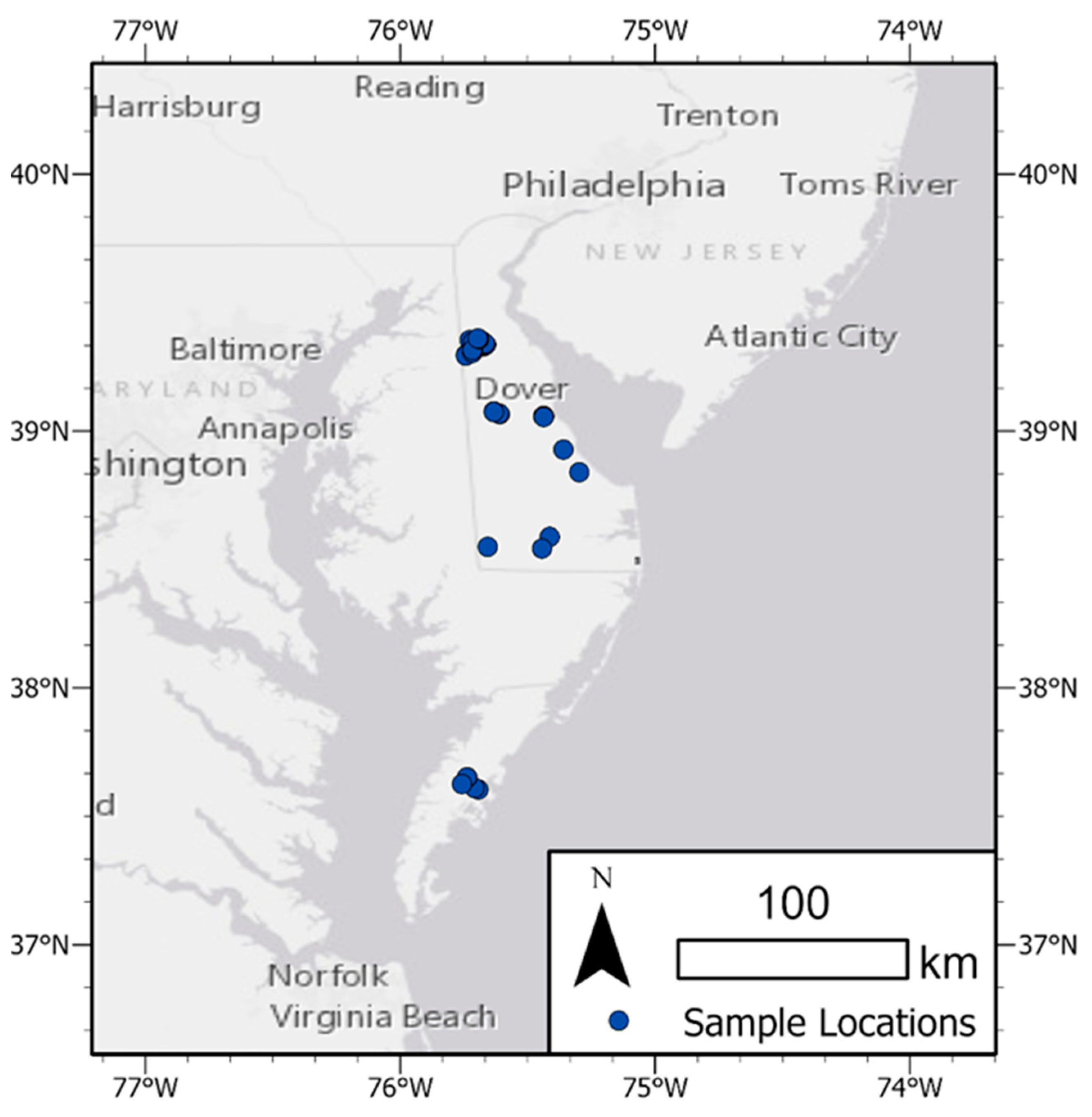
:1. Introduction
1.1. Past Studies on Carolina Bays
1.2. Past Population Estimates of Carolina Bays
1.3. Traditional Computer Vision, Pixel-Based Classification, and Object Detection
2. Materials and Methods
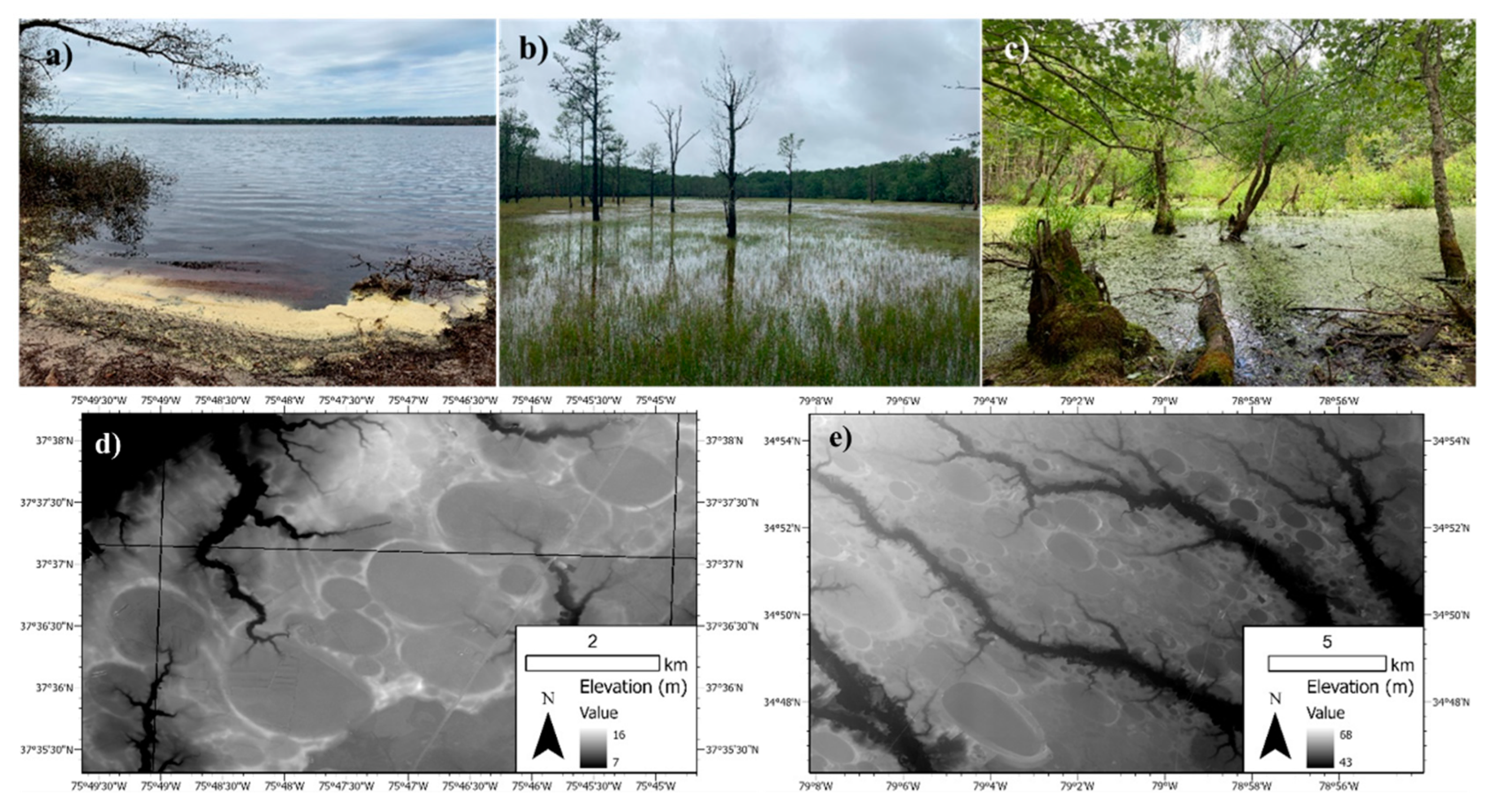
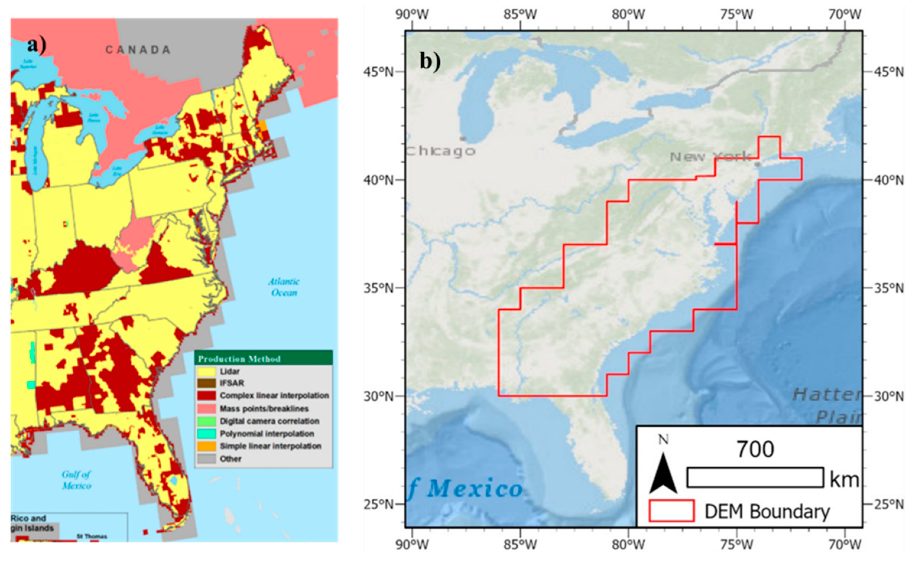
2.1. Data Sources
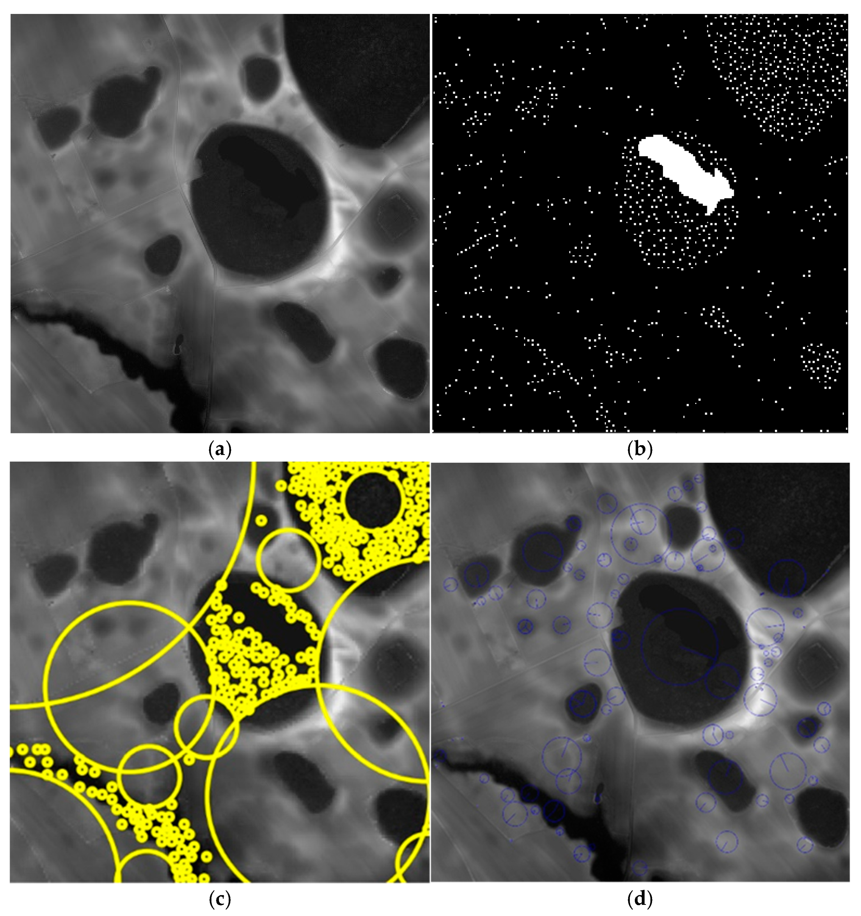
2.2. Building the Annotation Datasets
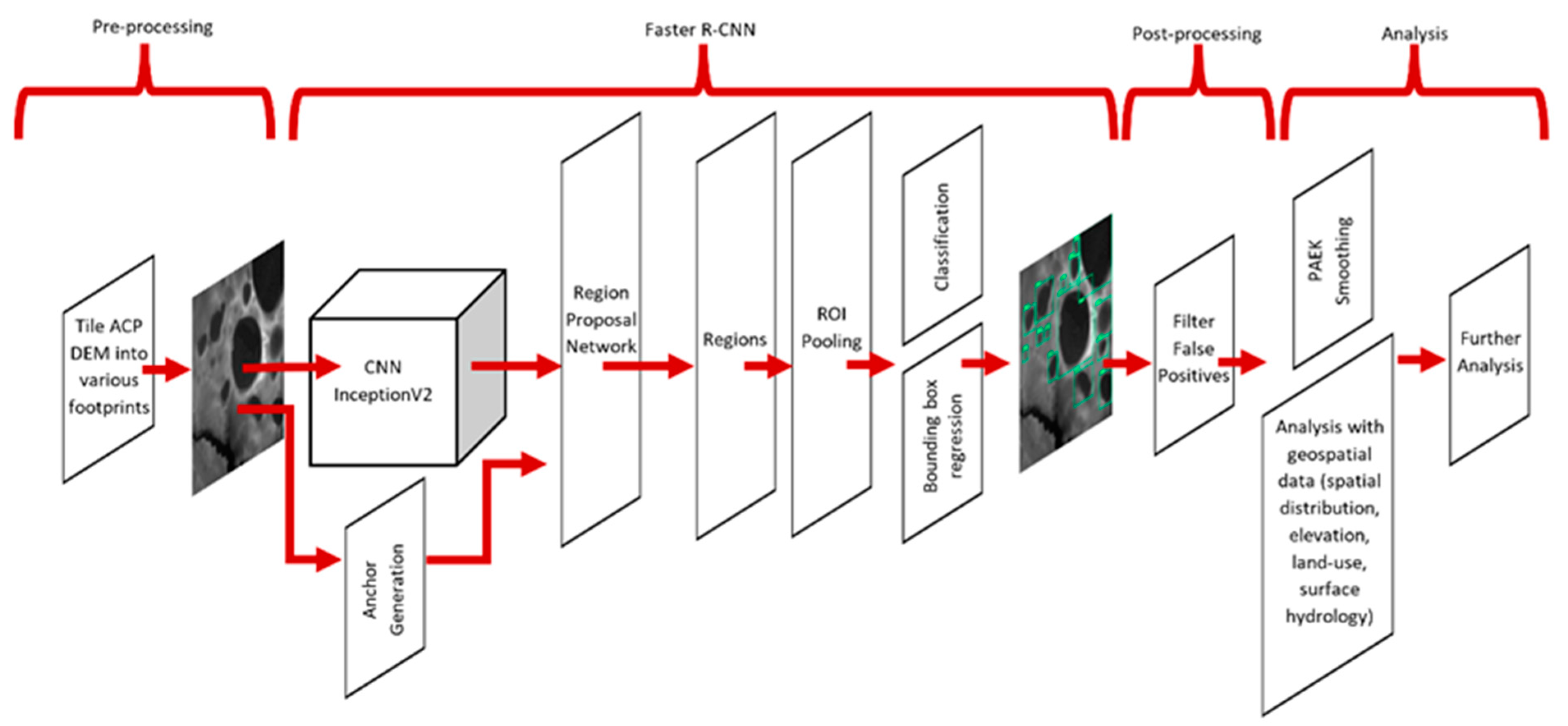
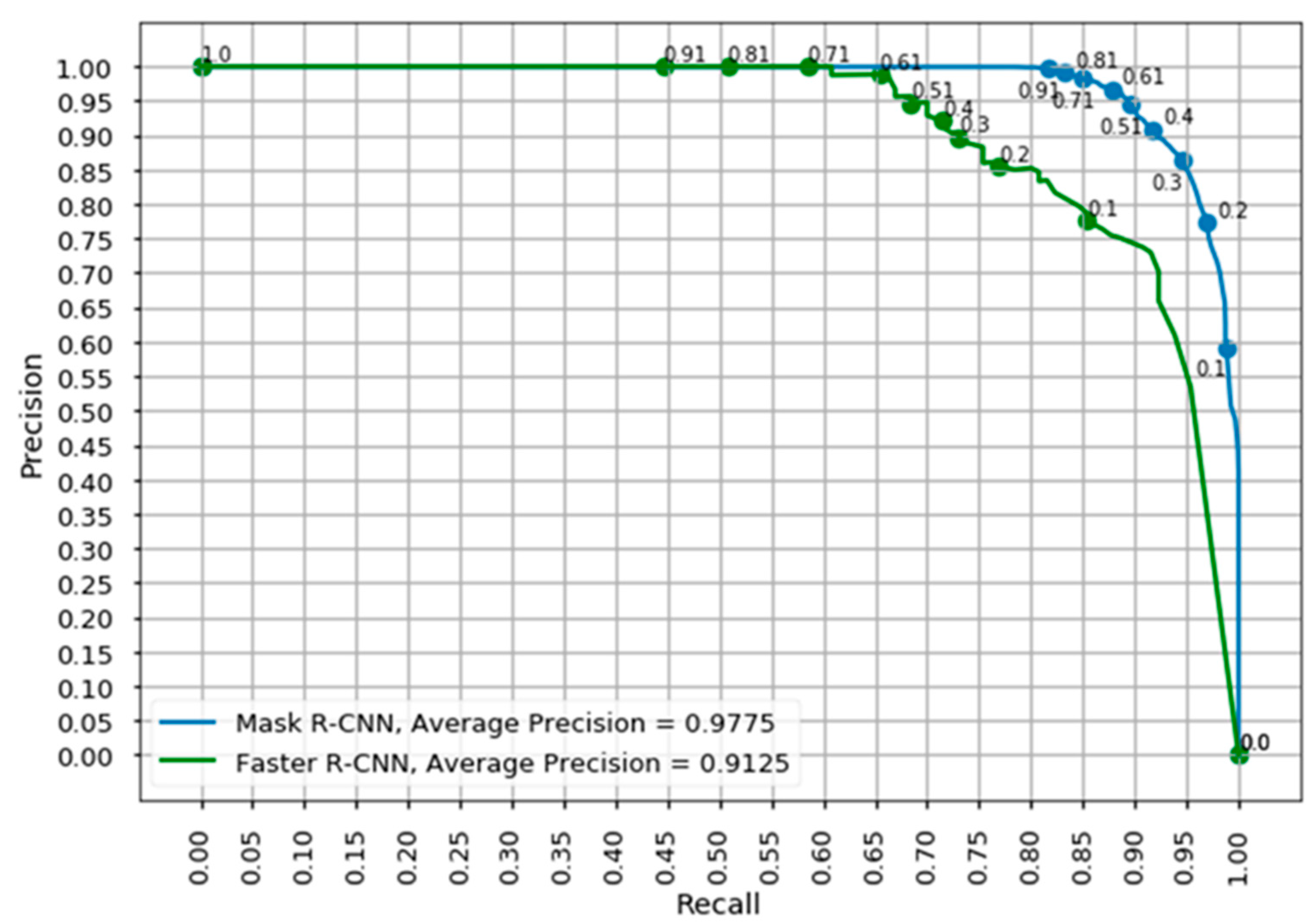
2.3. Training the CNNs and Assessing Accuracy
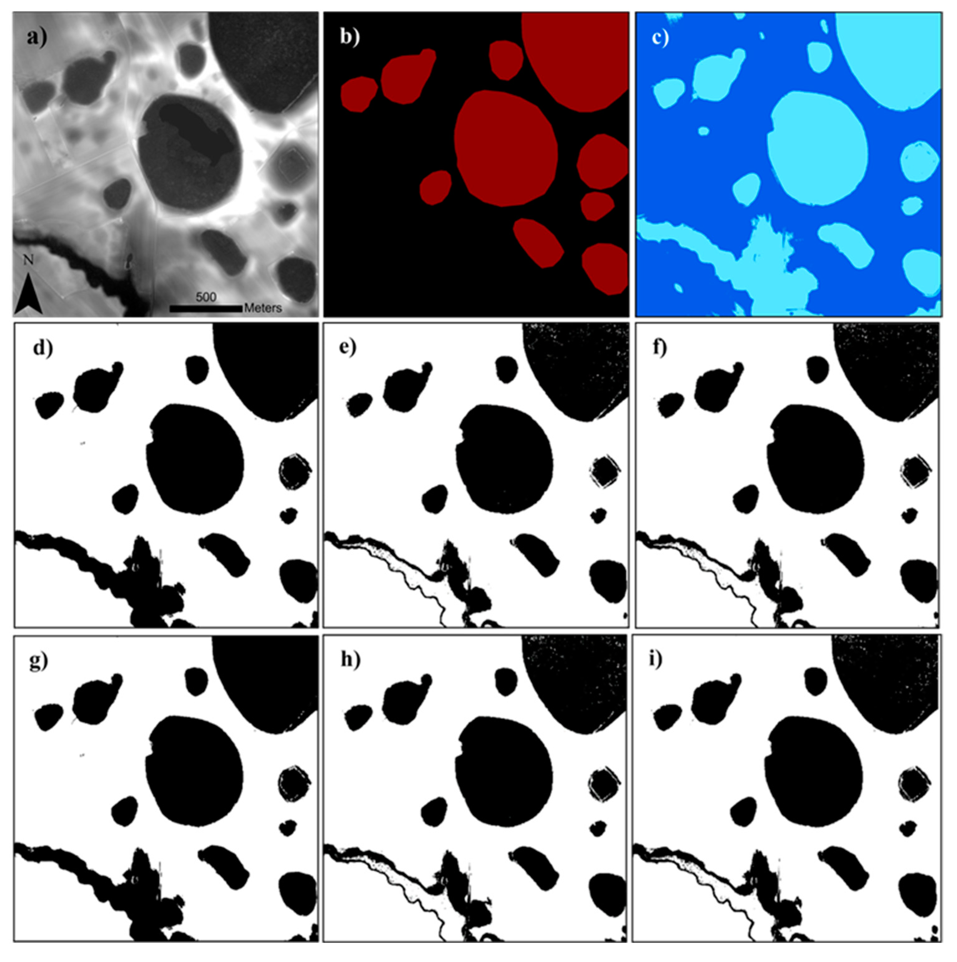
2.4. Extracting Morphologic, LULC, and Hydrologic Parameters from Detections
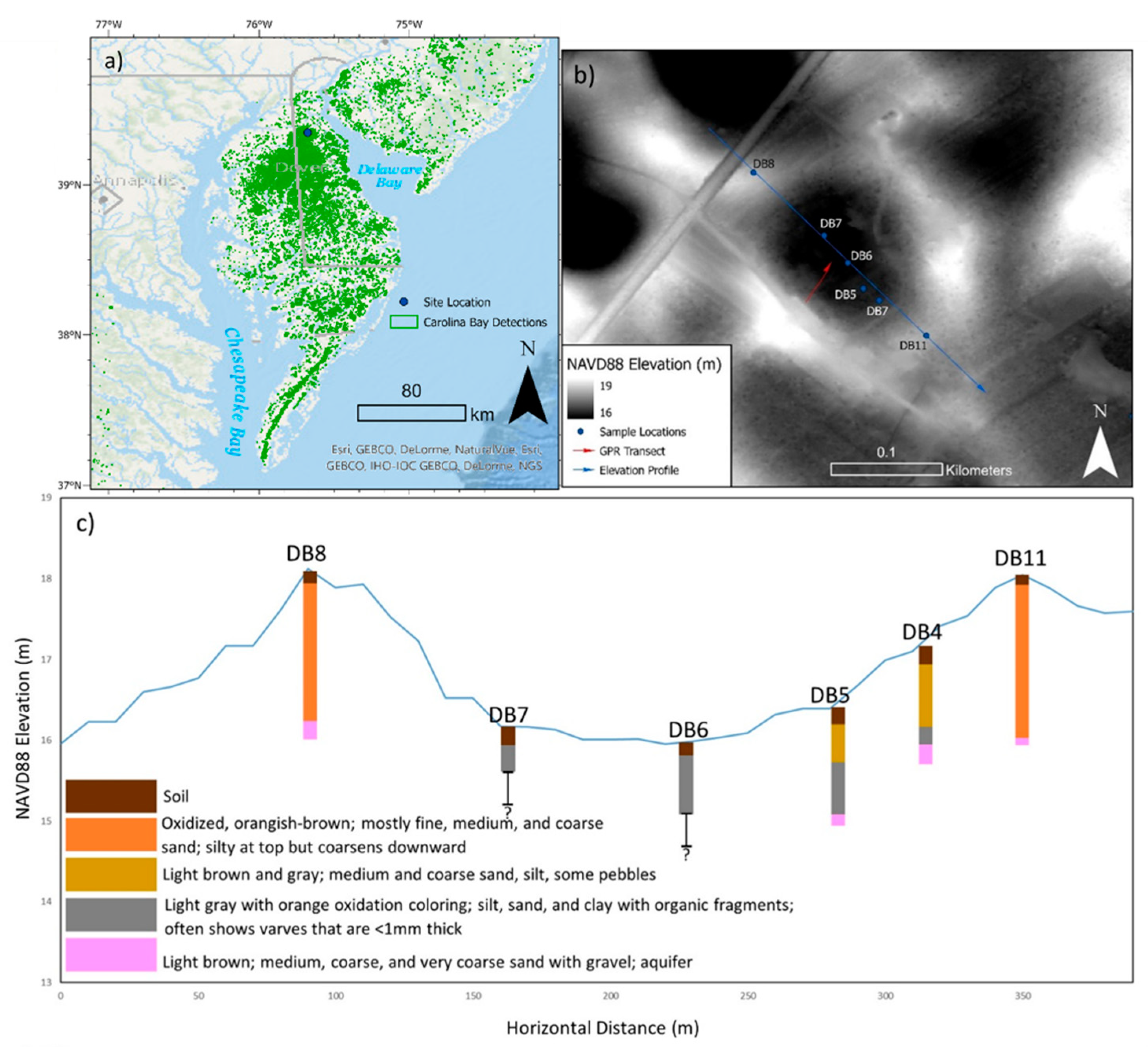
2.5. Field Investigations Based on Detection Results
2.6. Principal Component Analysis of Topographic Metrics
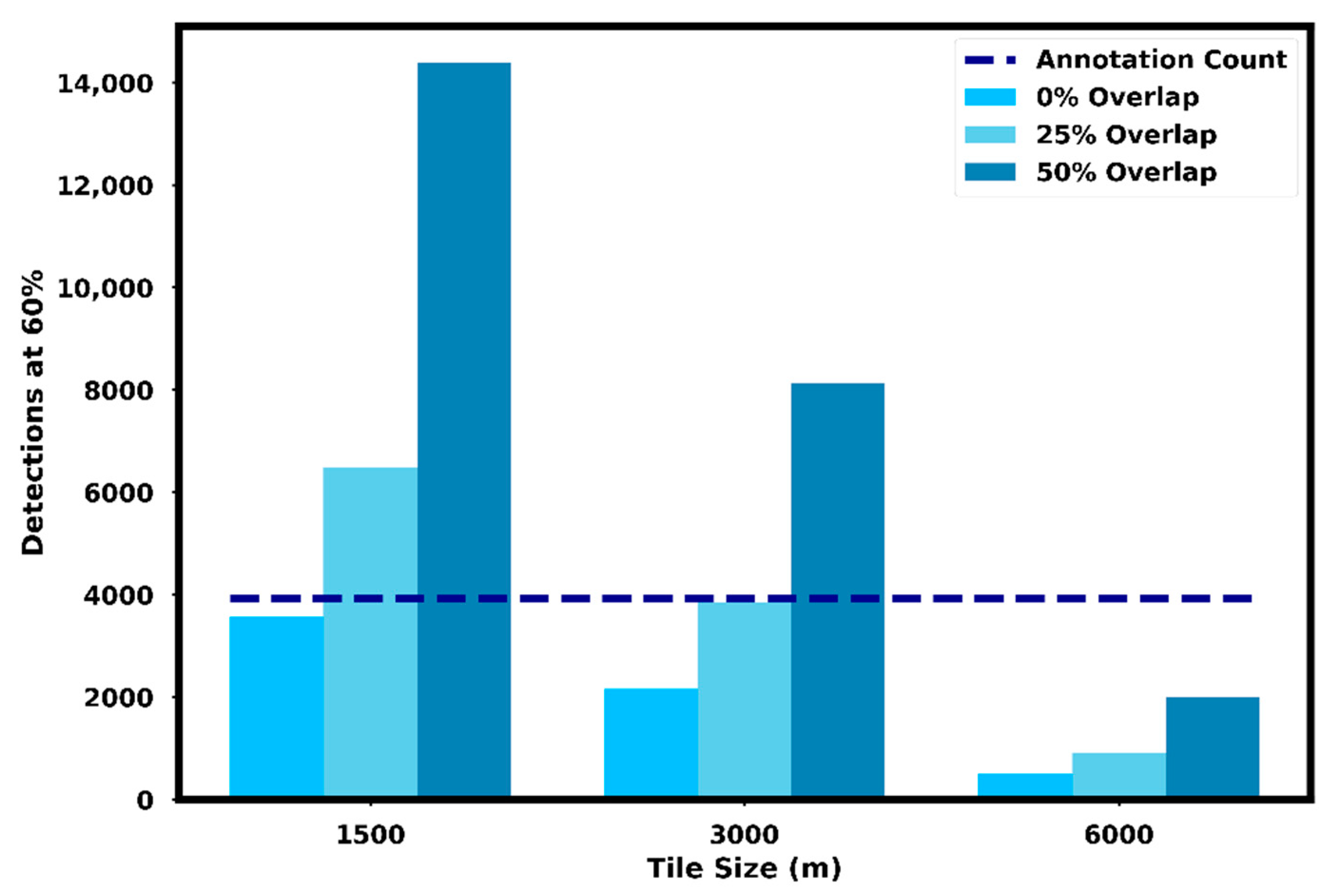
2.7. Multi-Scale Detection, Aggregation, and Smoothing
3. Results
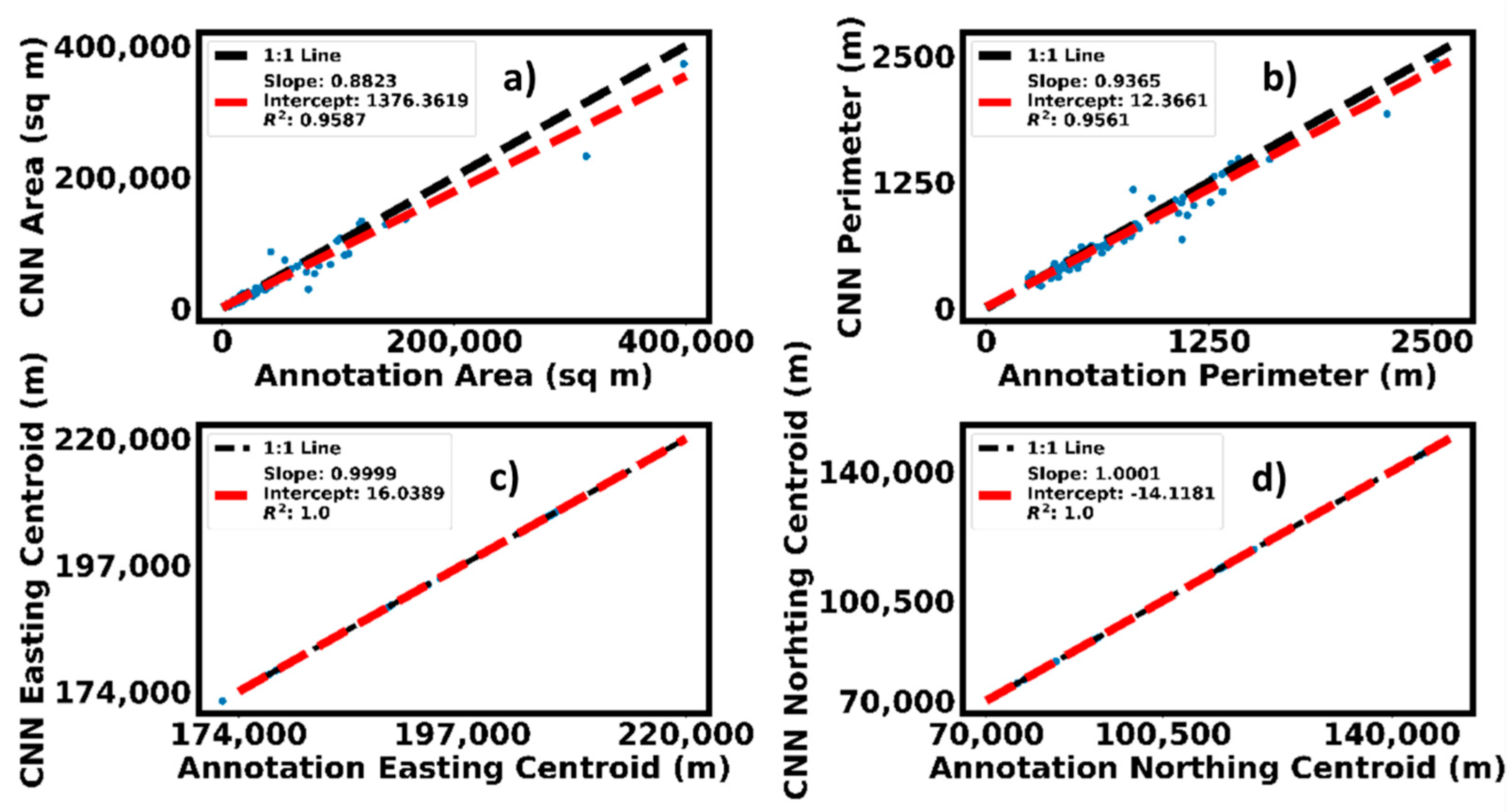
3.1. Assessment of Detection Results
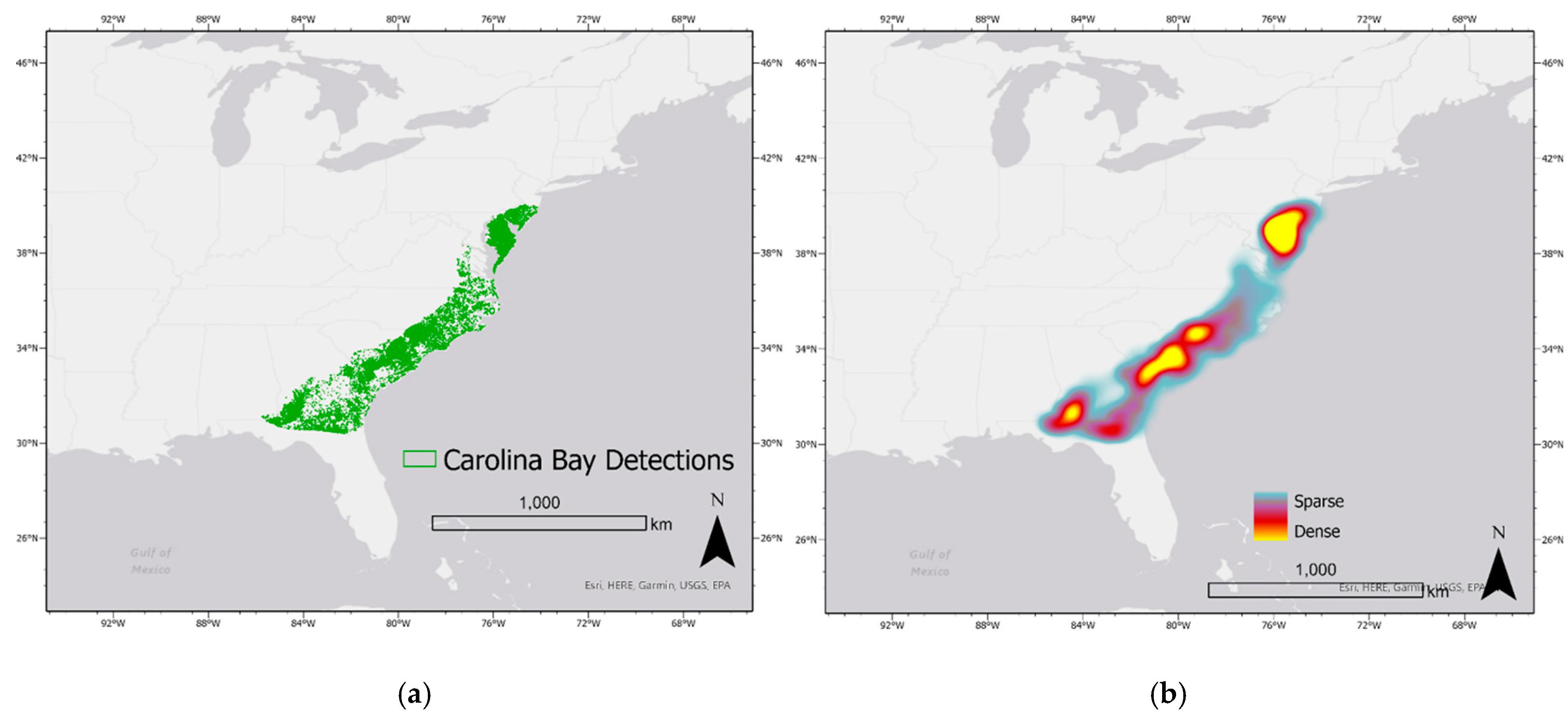
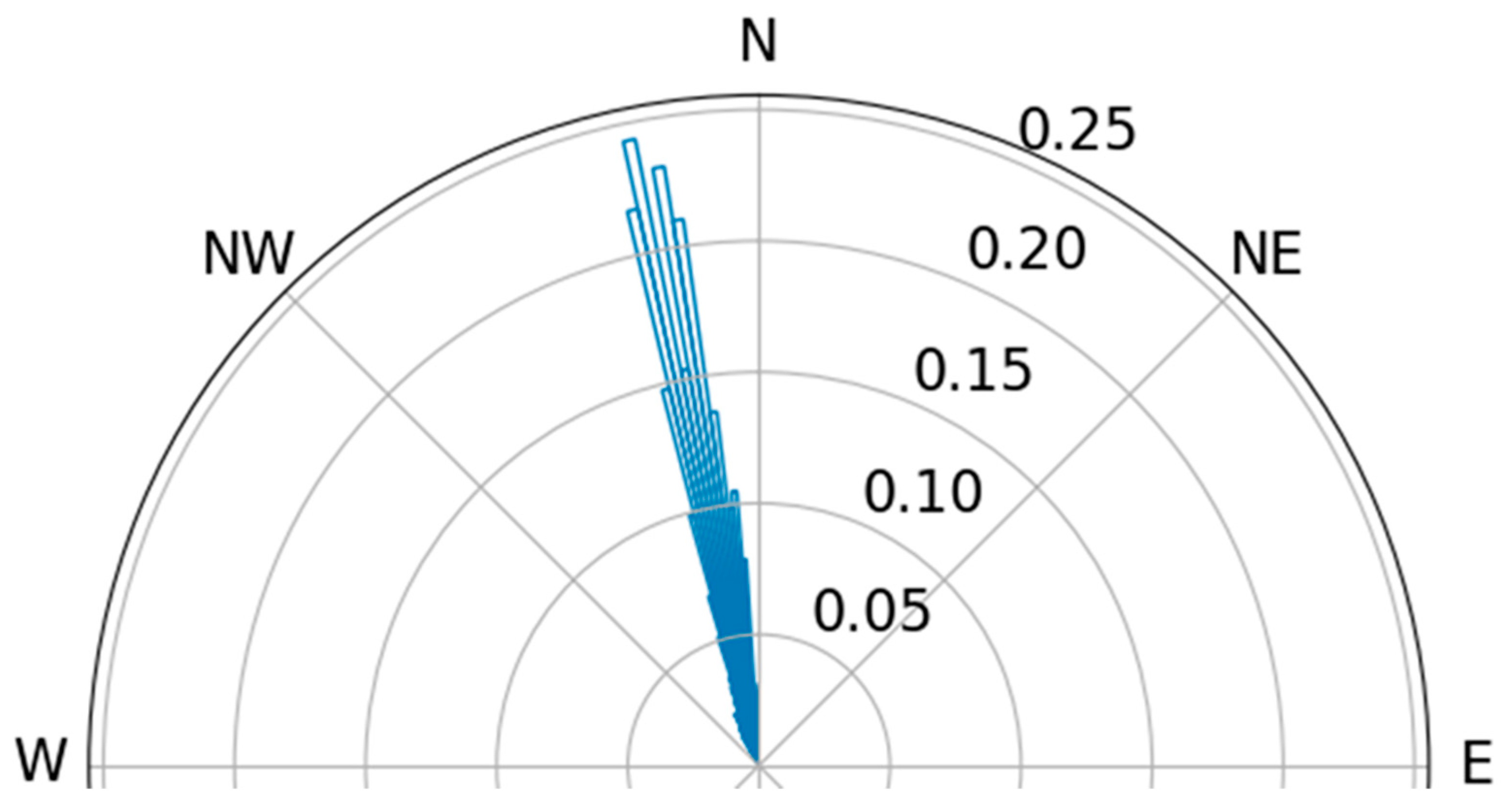
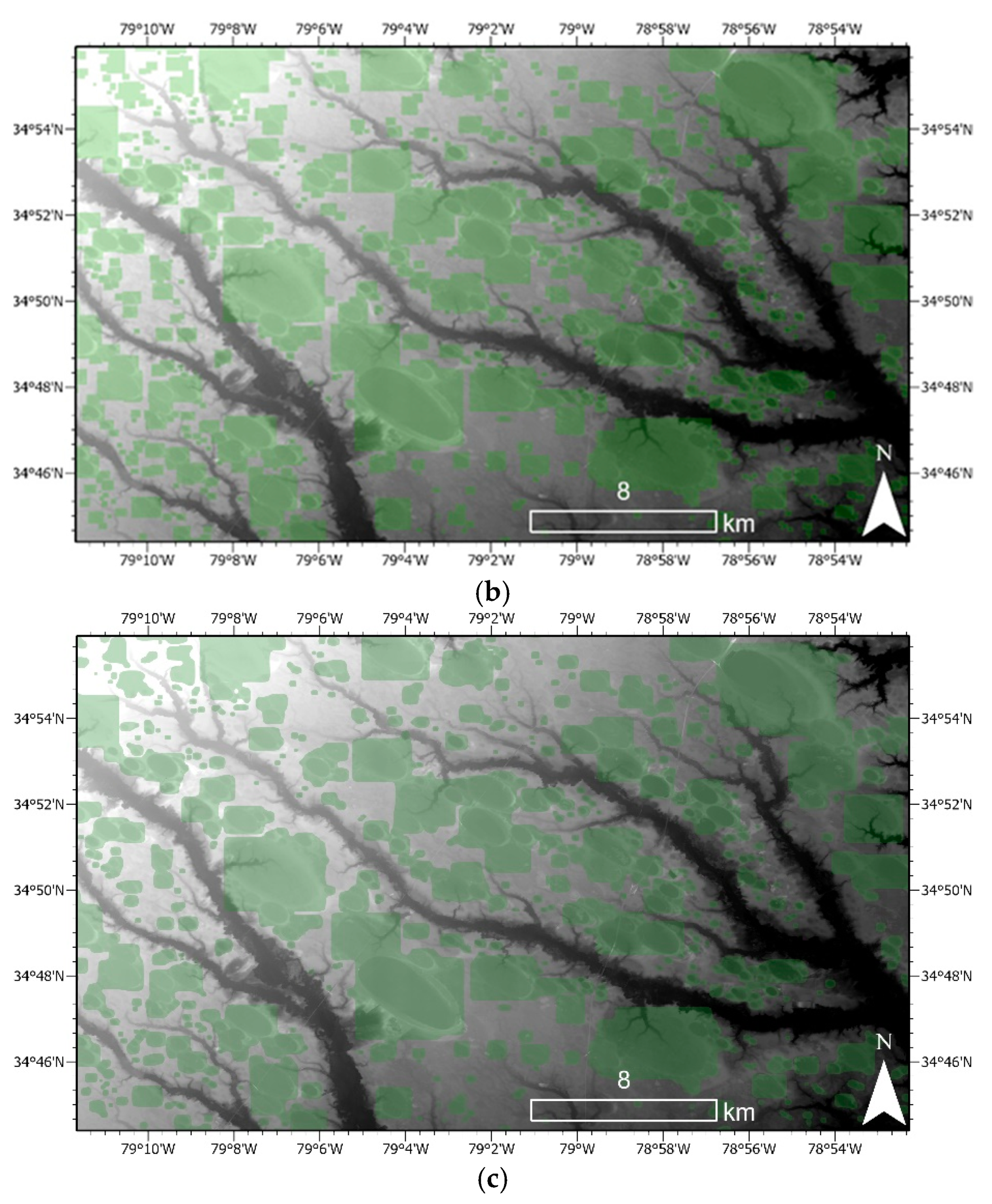
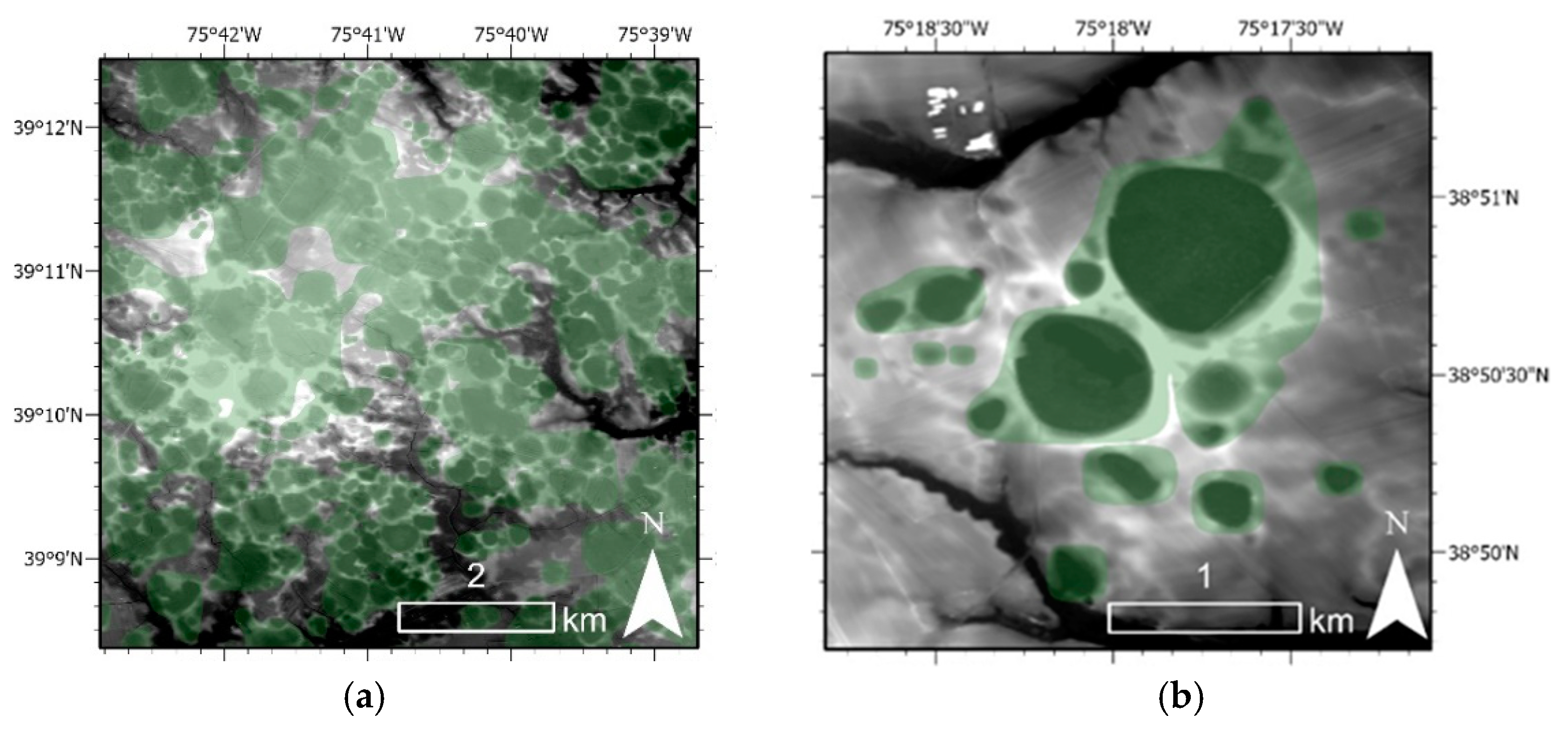
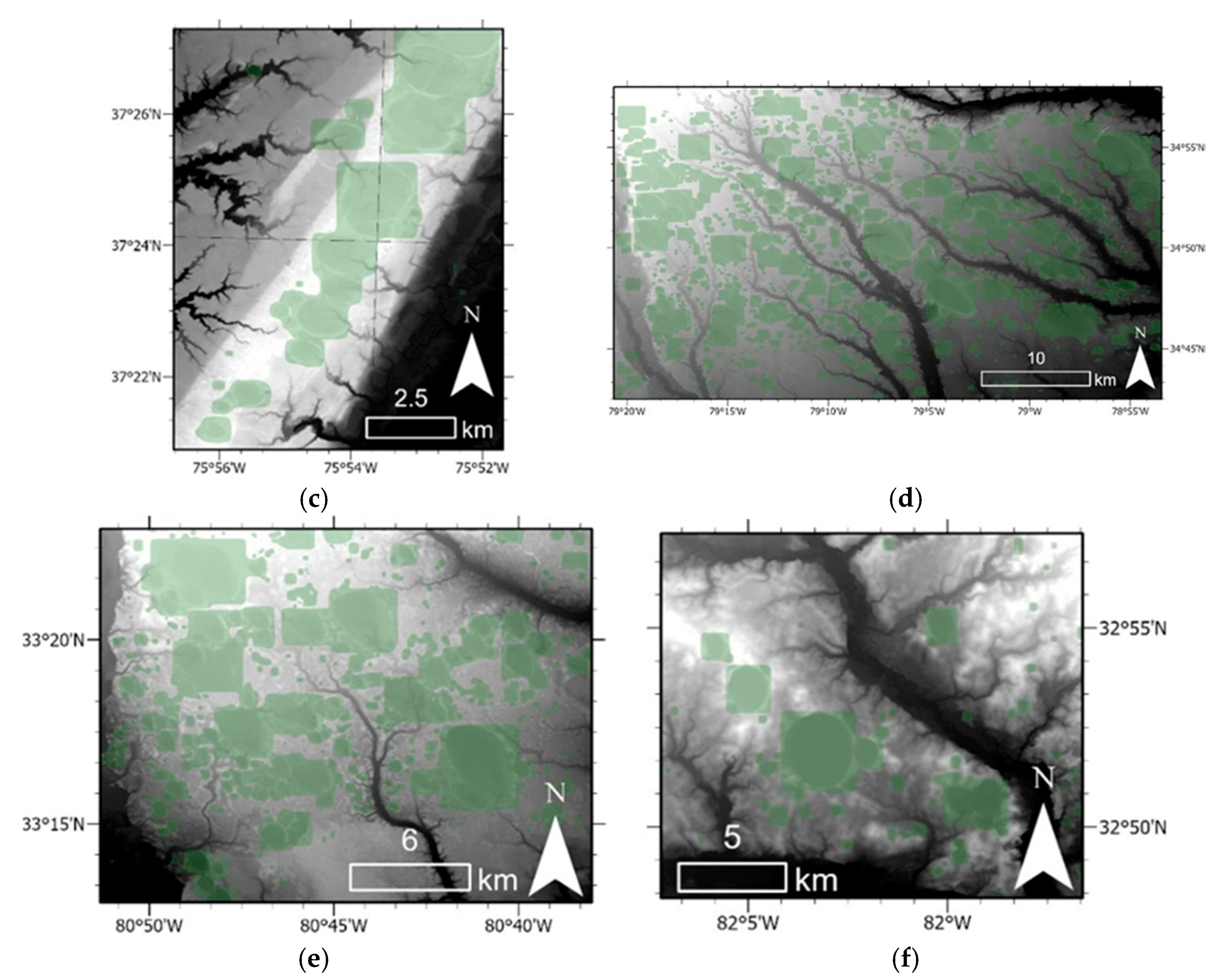
3.2. Spatial Distribution of Carolina Bay Detections
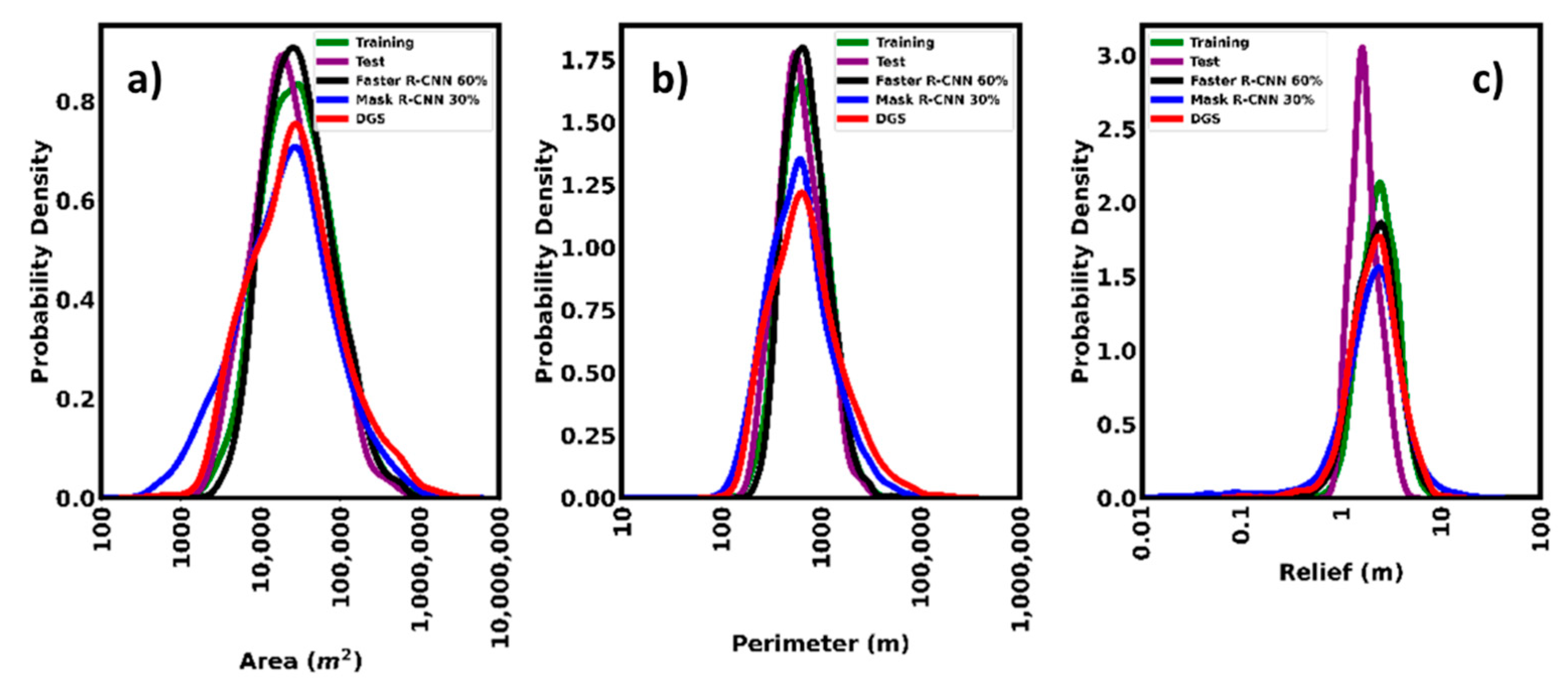
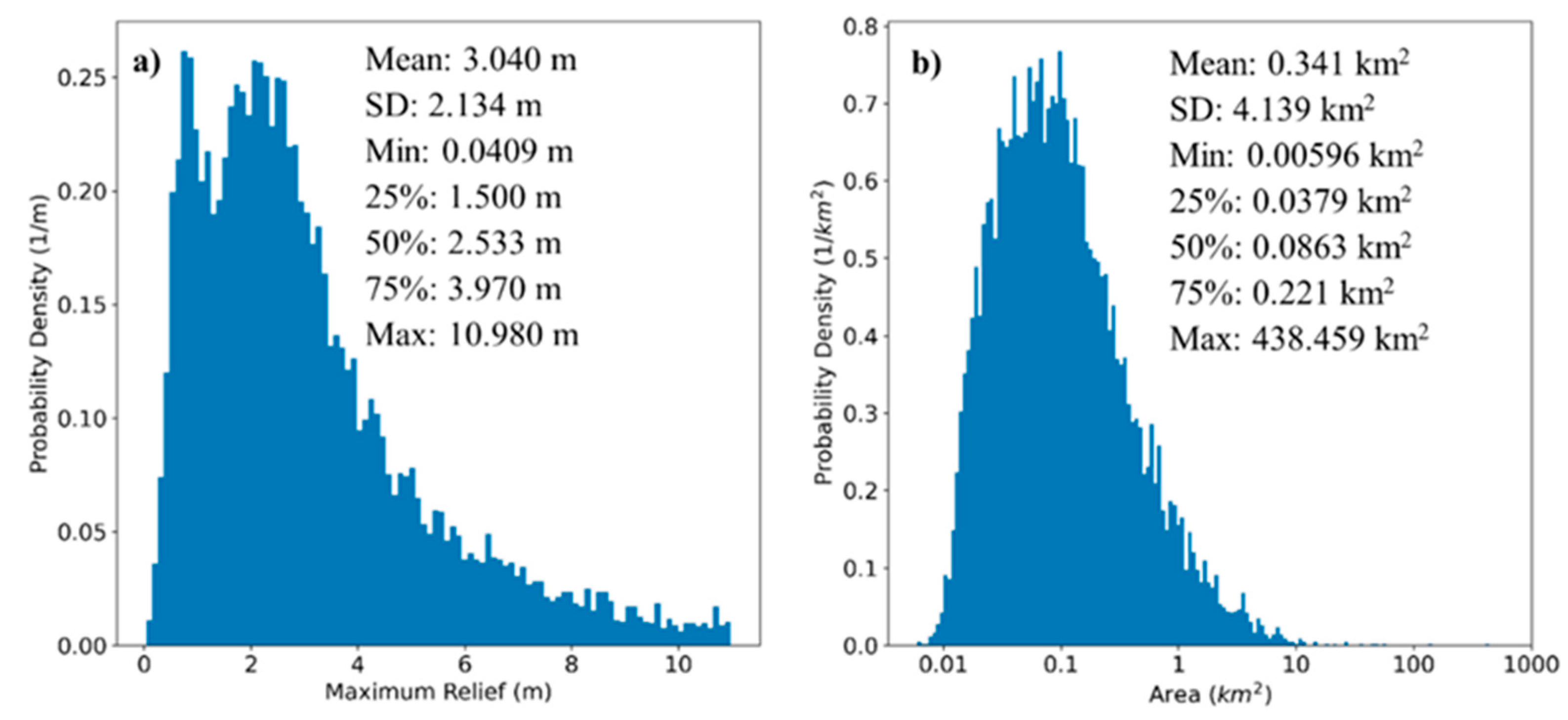
3.3. Morphology of Carolina Bay Detections
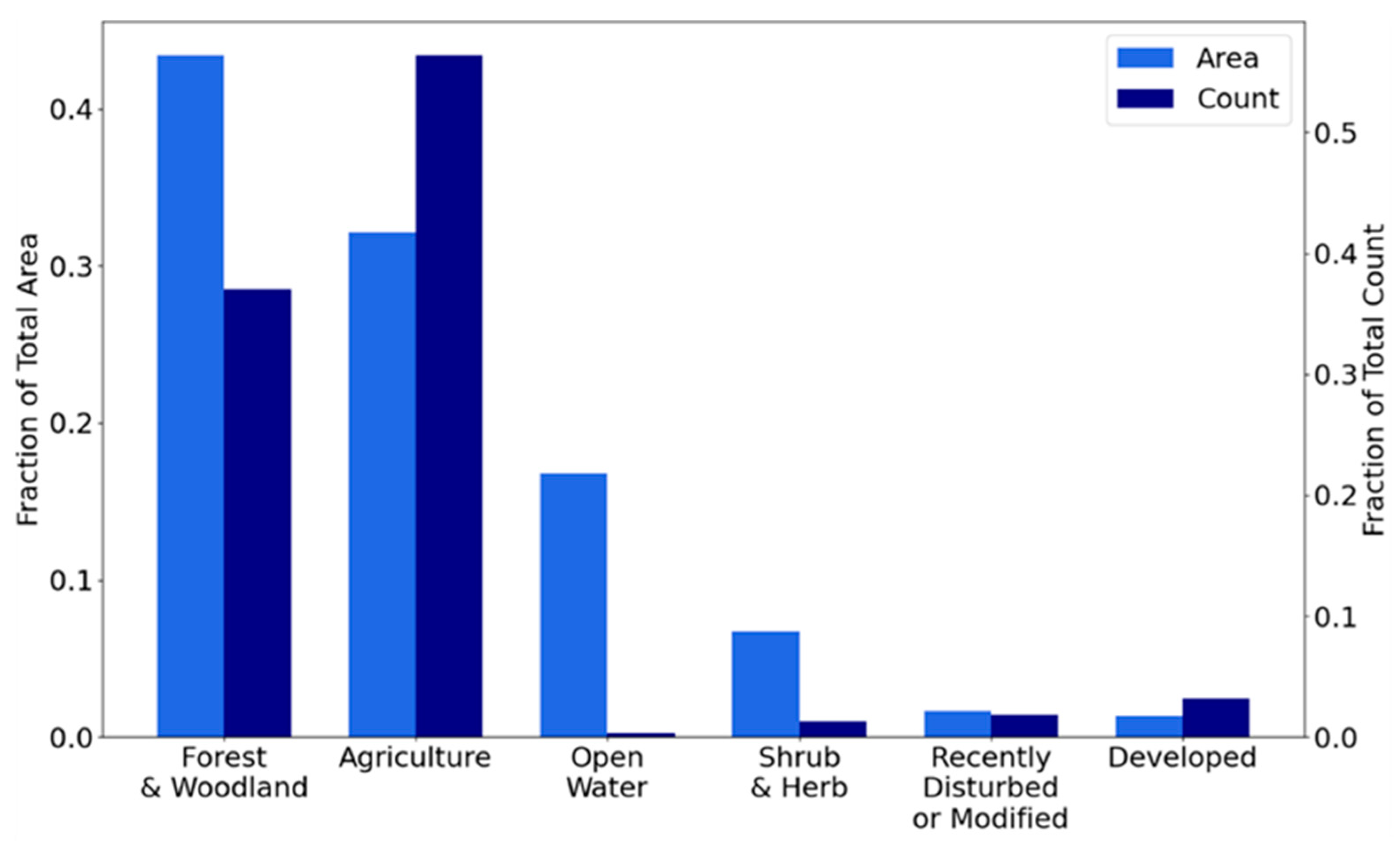
3.4. LULC of Carolina Bay Detections
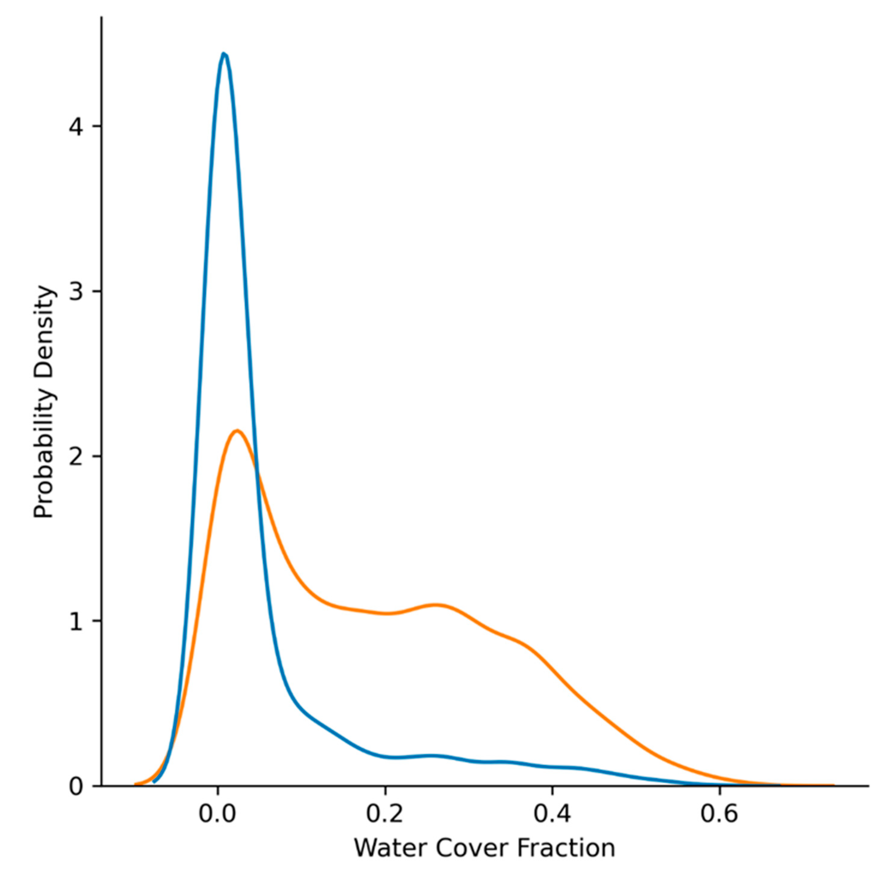
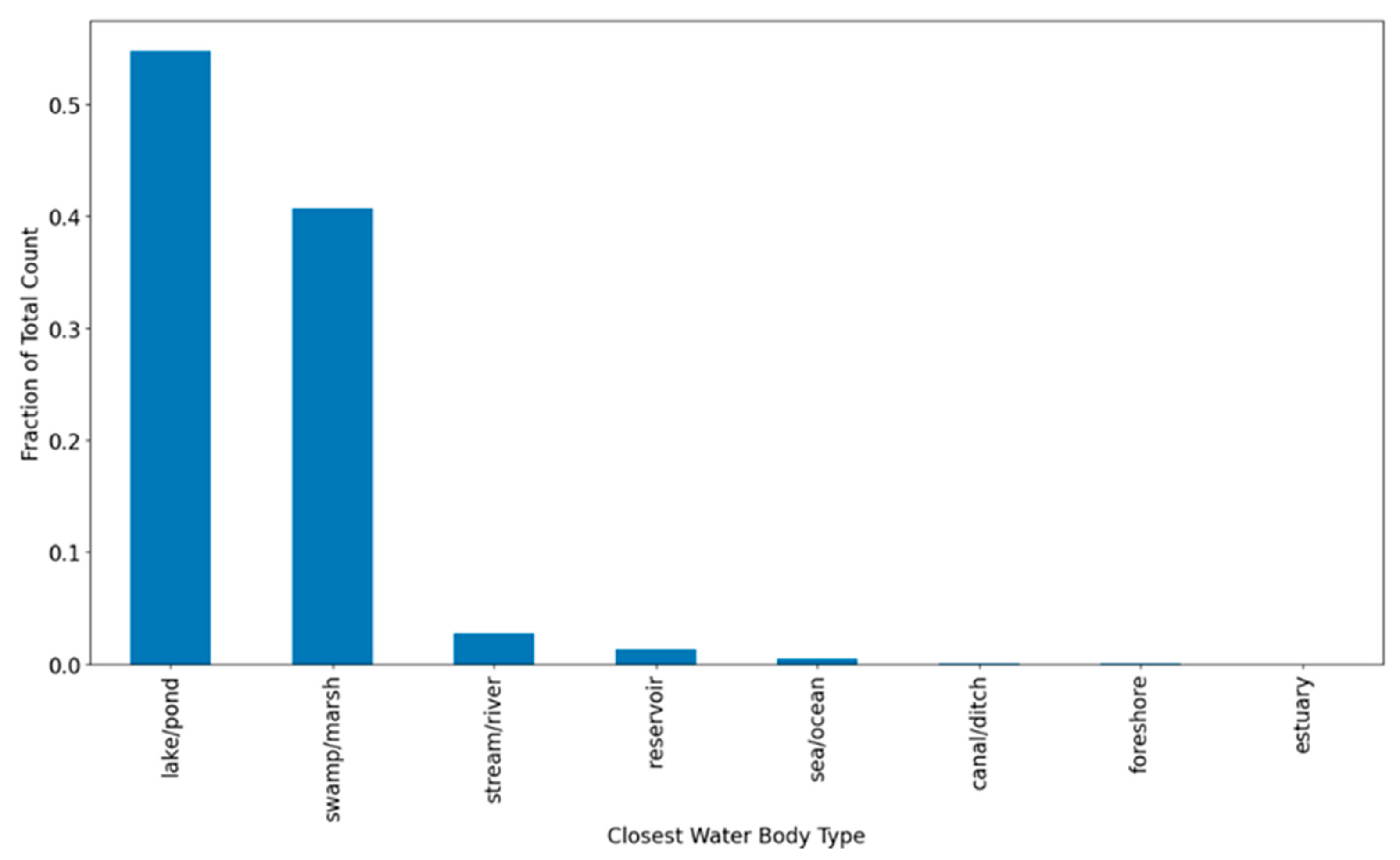
3.5. Hydrology of Carolina Bay Detections
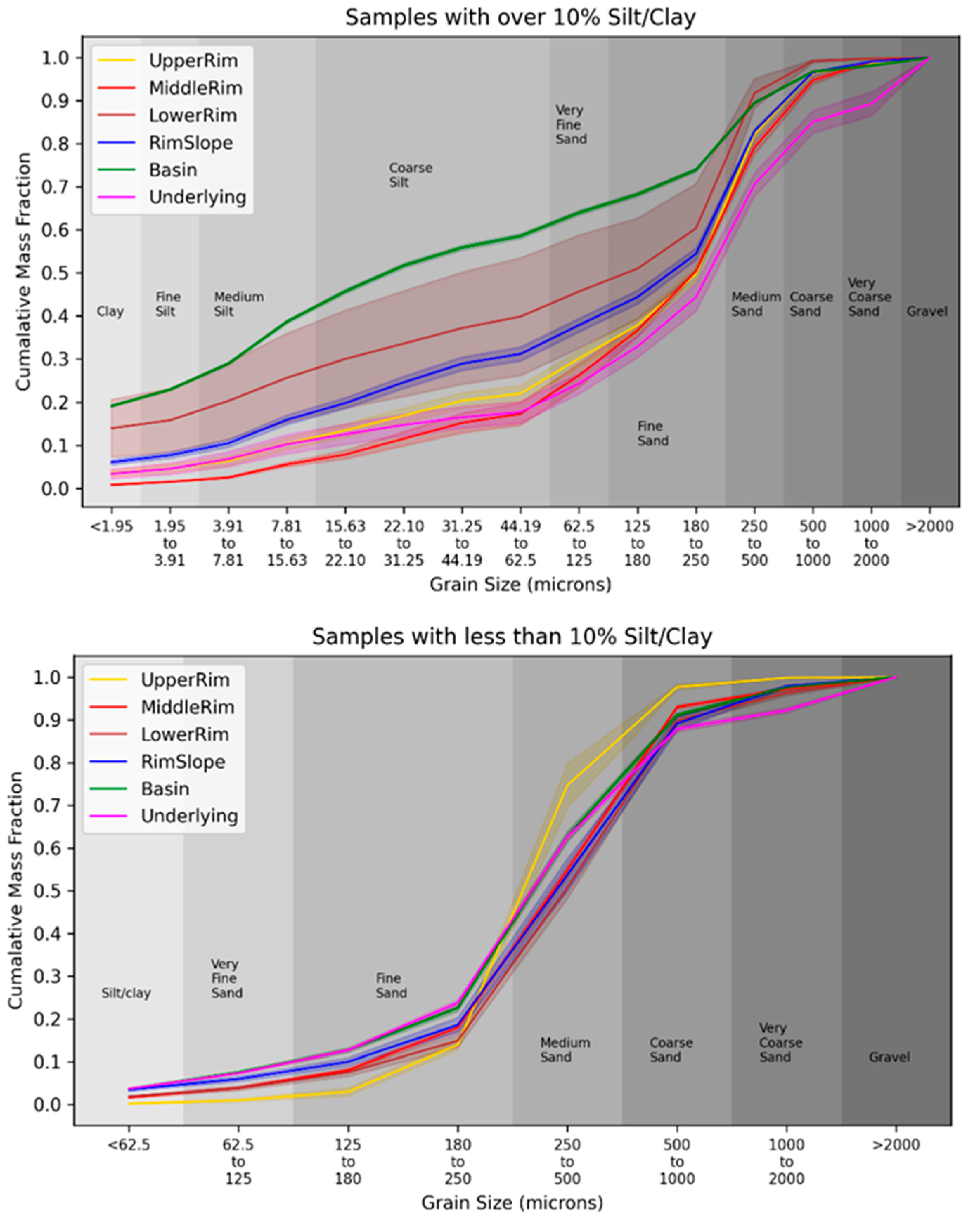
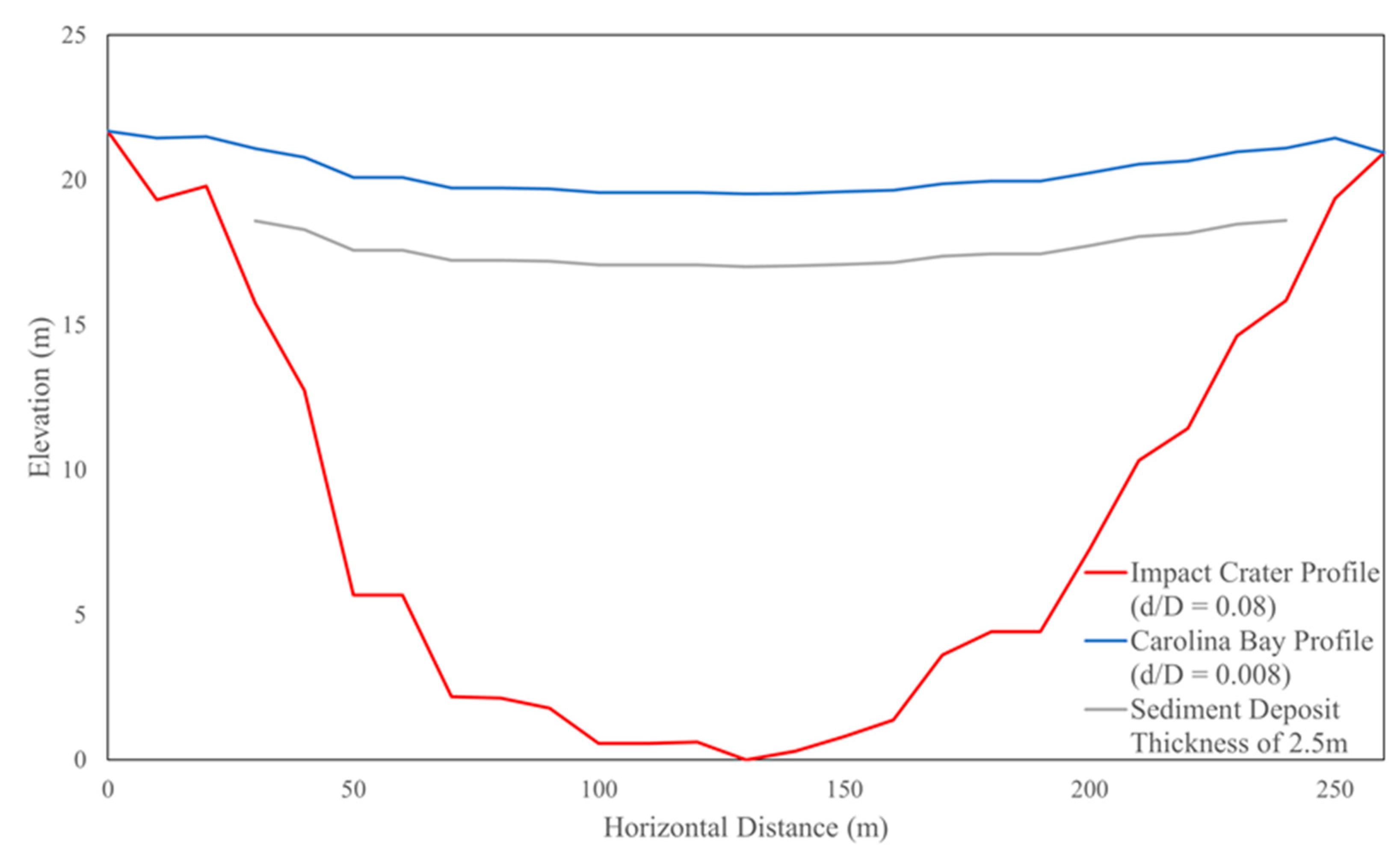
3.6. Sedimentology of Carolina Bays
3.7. Principal Component Analysis of Topographic Metrics
3.8. Multi-Scale Detection, Aggregation, and Smoothing
4. Discussion
5. Conclusions
Supplementary Materials
Author Contributions
Funding
Institutional Review Board Statement
Informed Consent Statement
Data Availability Statement
Acknowledgments
Conflicts of Interest
References
- Cooke, C.W.; Melton, F.A. Discussion of the Origin of the Supposed Meteorite Scars of South Carolina. J. Geol. 1934, 42, 88–104. [Google Scholar] [CrossRef]
- Eyton, J.R.; Parkhurst, J.I. A Re-Evaluation of the Extraterrestrial Origin of the Carolina Bays; Geography Graduate Student Association, University of Illinois: Urbana Champaign, IL, USA, 1975. [Google Scholar]
- Firestone, R.B.; West, A.; Kennett, J.P.; Becker, L.; Bunch, T.E.; Revay, Z.S.; Schultz, P.H.; Belgya, T.; Kennett, D.J.; Erlandson, J.M.; et al. Evidence for an extraterrestrial impact 12,900 years ago that contributed to the megafaunal extinctions and the Younger Dryas cooling. Proc. Natl. Acad. Sci. USA 2007, 104, 16016–16021. [Google Scholar] [CrossRef]
- Melton, F.A.; Schriver, W. The Carolina “Bays”: Are They Meteorite Scars? J. Geol. 1933, 41, 52–66. [Google Scholar] [CrossRef]
- Prouty, W.F. Carolina Bays and Their Origin. GSA Bull. 1952, 63, 167–224. [Google Scholar] [CrossRef]
- Zamora, A. A model for the geomorphology of the Carolina Bays. Geomorphology 2017, 282, 209–216. [Google Scholar] [CrossRef]
- Glenn, L.C. Some Notes on Darlington (S. C.), “Bays”. Science 1895, 2, 472–475. [Google Scholar] [CrossRef]
- Johnson, D.W. Role of Artesian Waters in Forming the Carolina Bays. Science 1937, 86, 255–258. [Google Scholar] [CrossRef] [PubMed]
- Johnson, D.W. The Origin of the Carolina Bays; Columbia University Press: New York, NY, USA, 1942. [Google Scholar]
- Kaczorowski, R.T. The Carolina Bays and Their Relationship to Modern Oriented Lakes. Unpublished Dissertation, University of South Carolina, Sumter, SC, USA, 1977. [Google Scholar]
- Kaczorowski, R.T. Origin of the Carolina Bays, Technical Report-Coastal Research Division; University of South Carolina: Sumter, SC, USA, 1976. [Google Scholar]
- Moore, C.R.; Brooks, M.J.; Mallinson, D.J.; Parham, P.R.; Ivester, A.H.; Feathers, J.K. The Quaternary evolution of Herndon Bay, a Carolina Bay on the Coastal Plain of North Carolina (USA): Implications for paleoclimate and oriented lake genesis. Southeast. Geol. 2016, 51, 145–171. [Google Scholar]
- Rodriguez, A.B.; Waters, M.N.; Piehler, M.F. Burning peat and reworking loess contribute to the formation and evolution of a large Carolina-bay basin. Quat. Res. 2012, 77, 171–181. [Google Scholar] [CrossRef]
- Smith, L.L. Solution depressions in sandy sediments of the Coastal Plain in South Carolina. J. Geol. 1931, 39, 641–652. [Google Scholar] [CrossRef]
- Thom, B.G. Carolina Bays in Horry and Marion Counties, South Carolina. GSA Bull. 1970, 81, 783–813. [Google Scholar] [CrossRef]
- Tuomey, M. Report on the Geology of South Carolina: Geological Survey of South Carolina; A.S. Johnston: Columbia, SC, USA, 1848. [Google Scholar]
- Tomlinson, J.L.; Ramsey, K.W. Stratigraphic, hydrologic, and climatic influences on the formation and spatial distribution of Carolina bays in central Delaware. In Proceedings of the 49th Annual Meeting of the Northeastern Section of the Geological Society of America, Lancaster, PA, USA, 23–25 March 2014. [Google Scholar]
- Brooks, M.J.; Taylor, B.E.; Grant, J.A. Carolina Bay geoarchaeology and Holocene landscape evolution on the Upper Coastal Plain of South Carolina. Geoarchaeology 1996, 11, 481–504. [Google Scholar] [CrossRef]
- Brooks, M.J.; Taylor, B.E.; Ivester, A.H. Carolina bays: Time capsules of culture and climate change. Southeast. Archaeol. 2010, 29, 146–163. [Google Scholar] [CrossRef]
- Brooks, M.J.; Taylor, B.E.; Stone, P.A.; Gardner, L.R. Pleistocene encroachment of the Wateree River sand sheet into Big Bay on the middle Coastal Plain of South Carolina. Southeast. Geol. 2001, 40, 241–257. [Google Scholar]
- Hussey, T.C. A 20,000 Year History of Vegetation and Climate at Clear Pond, Northeastern South Carolina. Unpublished Master’s Thesis, University of Maine, Orono, MA, USA, 1993. [Google Scholar]
- Ivester, A.H.; Brooks, M.J.; Taylor, B.E. Sedimentology and ages of Carolina bay sand rims. Geol. Soc. Am. Abstr. Programs 2007, 39, 5. [Google Scholar]
- Ivester, A.H.; Poplin, E.C.; Brooks, M.J.; Brook, G.A. Life on the edge: The formation of Mathis Lake and its human occupation. South Carol. Antiq. 2009, 41, 1–16. [Google Scholar]
- Ramsey, K.W.; Baxter, S.J. Radiocarbon Dates from Delaware: A Compilation; Delaware Geological Survey, University of Delaware: Newark, DE, USA, 1996; pp. 1–18. [Google Scholar]
- Watts, W.A. Late-Quaternary Vegetation History at White Pond on the Inner Coastal Plain of South Carolina. Quat. Res. 1980, 13, 187–199. [Google Scholar] [CrossRef]
- Richardson, C.J.; Gibbons, J.W. Pocosins, Carolina Bays and Mountain Bogs. In Biodiversity of the Southeastern United States—Lowland Terrestrial Communities; Martin, W.H., Boyce, S.G., Echternacht, A.C., Eds.; Wiley: New York, NY, USA, 1993; pp. 257–310. [Google Scholar]
- Piovan, S.; Hodgson, M.E. How many Carolina bays? An analysis of Carolina bays from USGS topographic maps at different scales. Cartogr. Geogr. Inf. Sci. 2016, 44, 310–326. [Google Scholar] [CrossRef]
- Fenstermacher, D.E.; Rabenhorst, M.C.; Lang, M.W.; Mccarty, G.W.; Needelman, B.A. Distribution, Morphometry, and Land Use of Delmarva Bays. Wetlands 2014, 34, 1219–1228. [Google Scholar] [CrossRef]
- Gevana, D.; Camacho, L.; Carandang, A.; Camacho, S.; Im, S. Land use characterization and change detection of a small mangrove area in Banacon Island, Bohol, Philippines using a maximum likelihood classification method. For. Sci. Technol. 2015, 11, 197–205. [Google Scholar] [CrossRef]
- Otukei, J.R.; Blaschke, T. Land cover change assessment using decision trees, support vector machines and maximum likelihood classification algorithms. Int. J. Appl. Earth Obs. Geoinf. 2010, 12 (Suppl. 1), 27–31. [Google Scholar] [CrossRef]
- Sekovski, I.; Stecchi, F.; Mancini, F.; Del Rio, L. Image classification methods applied to shoreline extraction on very high-resolution multispectral imagery. Int. J. Remote. Sens. 2014, 35, 3556–3578. [Google Scholar] [CrossRef]
- Rasmussen, C.; Zhao, J.; Ferraro, D.; Trembanis, A. Deep Census: AUV-Based Scallop Population Monitoring. In Proceedings of the IEEE International Conference on Computer Vision Workshops (ICCVW), Venice, Italy, 22–29 October 2017; pp. 2865–2873. [Google Scholar]
- Hou, F.; Lei, W.; Li, S.; Xi, J.; Xu, M.; Luo, J. Improved Mask R-CNN with distance guided intersection over union for GPR signature detection and segmentation. Autom. Constr. 2021, 121, 103414. [Google Scholar] [CrossRef]
- Bonhage, A.; Eltaher, M.; Raab, T.; Breuß, M.; Raab, A.; Schneider, A. A modified Mask region-based convolutional neural network approach for the automated detection of archaeological sites on high-resolution light detection and ranging-derived digital elevation models in the North German Lowland. Archaeol. Prospect. 2021, 28, 177–186. [Google Scholar] [CrossRef]
- Zhang, W.; Witharana, C.; Liljedahl, A.K.; Kanevskiy, M. Deep convolutional neural networks for automated characterization of Artic ice-wedge polygons in very high spatial resolution aerial imagery. Remote. Sens. 2018, 10, 1487. [Google Scholar] [CrossRef]
- Chen, Z.; Scott, T.R.; Bearman, S.; Anand, H.; Keating, D.; Scott, C.; Arrowsmith, J.R.; Das, J. Geomorphological analysis using unpiloted aircraft systems, structure from motion, and deep learning. In Proceedings of the IEEE/RSJ International Conference on Intelligent Robots and Systems (IROS), Las Vegas, NV, USA, 24 October–24 January 2021; pp. 1276–1283. [Google Scholar]
- Maxwell, A.E.; Pourmohammadi, P.; Poyner, J.D. Mapping the Topographic Features of Mining-Related Valley Fills Using Mask R-CNN Deep Learning and Digital Elevation Data. Remote Sens. 2020, 12, 547. [Google Scholar] [CrossRef]
- Guo, W.; Yang, W.; Zhang, H.; Hua, G. Geospatial Object Detection in High Resolution Satellite Images Based on Multi-Scale Convolutional Neural Network. Remote. Sens. 2018, 10, 131. [Google Scholar] [CrossRef]
- Bochkovskiy, A.; Wang, C.; Liao, H.M. YOLOv4: Optimal speed and accuracy of object detection. arXiv 2020, arXiv:2004.10934. [Google Scholar]
- O’Mahony, N.; Campbell, S.; Carvalho, A.; Harapanahalli, S.; Hernandez, G.V.; Krpalkova, L.; Riordan, D.; Walsh, J. Deep Learning vs. Traditional Computer Vision. In Advances in Computer Vision; Springer International Publishing: Cham, Switzerland, 2019; pp. 128–144. [Google Scholar]
- Campagnolo, M.L.; Cerdeira, J.O. Contextual classification of remotely sensed images with integer linear programming. In CompIMAGE. Computational Modeling of Objects Represented in Images: Fundamentals, Methods, and Applications; Taylor and Francis: London, UK, 2007; pp. 123–128. [Google Scholar]
- de Jong, S.M.; Hornstra, T.; Maas, H.-G. An integrated spatial and spectral approach to the classification of Mediterranean land cover types: The SSC method. Int. J. Appl. Earth Obs. Geoinf. 2001, 3, 176–183. [Google Scholar] [CrossRef]
- Gao, Y.; Mas, J.F. A comparison of the performance of pixel-based and object-based classifications over images with various spatial resolutions. Online J. Earth Sci. 2008, 2, 27–35. [Google Scholar]
- Van de Voorde, T.; De Genst, W.; Canters, F.; Stephenne, N.; Wolff, E.; Binard, M. Extraction of land use/land correlated information from very high resolution data in urban and suburban areas, Remote Sensing in Transition. In Proceedings of the 23rd Symposium of the European Association of Remote Sensing Laboratories, Rotterdam, The Netherlands, 2–5 June 2003; pp. 237–244. [Google Scholar]
- Weih, R.; Riggan, N. Object-based classification vs. Pixel-based classification: Comparitive importance of multi-resolution imagery. Int. Arch. Photogramm. Remote. Sens. Spat. Inf. Sci. ISPRS Arch. 2010, 38, C7. [Google Scholar]
- Ren, S.; He, K.; Girshick, R.; Sun, J. Faster R-CNN: Towards Real-Time Object Detection with Region Proposal Networks. arXiv 2015, arXiv:1506.01497. [Google Scholar] [CrossRef] [PubMed]
- He, K.; Gkioxari, G.; Dollár, P.; Girshick, R. Mask R-CNN. arXiv 2018, arXiv:1703.06870. [Google Scholar]
- Redmon, J.; Divvala, S.; Girshick, R.; Farhadi, A. You Only Look Once: Unified, Real-Time Object Detection. In Proceedings of the IEEE Conference on Computer Vision and Pattern Recognition (CVPR), Las Vegas, NV, USA, 27–30 June 2016; pp. 779–788. [Google Scholar]
- OCM Partners. 2014 USGS CMGP Lidar: Sandy Restoration (Delaware and Maryland). Available online: https://inport.nmfs.noaa.gov/inport/item/49662 (accessed on 1 August 2019).
- Virginia Department of Mines, Minerals and Energy (DMME). Virginia GIS Clearinghouse. Available online: https://vgin.maps.arcgis.com/home/index.html (accessed on 1 January 2020).
- Maryland iMap. Maryland’s Mapping and GIS Portal Lidar Download. Available online: https://imap.maryland.gov/Pages/lidar-download.aspx (accessed on 1 January 2020).
- U.S. Geological Survey. The National Map. Available online: https://www.usgs.gov/core-science-systems/national-geospatial-program/national-map (accessed on 1 January 2020).
- Tzutalin; LabelImg. Git Code 2015. Available online: https://github.com/tzutalin/labelImg (accessed on 1 August 2019).
- Delaware Geological Survey (DGS). DGS Digital Datasets. Available online: https://www.dgs.udel.edu/data (accessed on 1 August 2019).
- U.S. Geological Survey Gap Analysis Program. GAP/LANDFIRE National Terrestrial Ecosystems 2011. U.S. Geological Survey. 2016. Available online: https://www.sciencebase.gov/catalog/item/573cc51be4b0dae0d5e4b0c5 (accessed on 1 January 2020).
- U.S. Geological Survey. National Hydrography Dataset. Available online: https://www.usgs.gov/core-science-systems/ngp/national-hydrography (accessed on 1 February 2021).
- U.S. Environmental Protection Agency and U.S. Army Corps of Engineers. Clean Water Rule: Definition of “Waters of the United States”. 2015. Available online: https://www.epa.gov/sites/default/files/2015-05/documents/technical_support_document_for_the_clean_water_rule_1.pdf (accessed on 1 August 2021).
- U.S. Environmental Protection Agency and U.S. Army Corps of Engineers. The Navigable Waters Protection Rule: Definition of “Waters of the United States”. 2020. Available online: https://www.federalregister.gov/documents/2020/04/21/2020-02500/the-navigable-waters-protection-rule-definition-of-waters-of-the-united-states (accessed on 1 August 2021).
- Howell, N.; Krings, A.; Braham, R.R. Guide to the littoral zone vascular flora of Carolina bay lakes (U.S.A.). Biodivers. Data J. 2016, 4, e7964. [Google Scholar]
- Semlitsch, R. Size does matter: The value of small isolated wetlands. Natl. Wetl. Newsl. 2000, 22, 5–6, 13–14. [Google Scholar]
- Spadafora, E.; Leslie, A.W.; Culler, L.E.; Smith, R.F.; Staver, K.W.; Lamp, W.O. Macroinvertebrate community convergence between natural, rehabilitated, and created wetlands. Restor. Ecol. 2016, 24, 463–470. [Google Scholar] [CrossRef]
- Van De Genachte, E.; Cammack, S. Carolina Bays of Georgia, Their Distribution, Condition, And Conservation; Georgia Natural Heritage Program, Wildlife Resources Division: SE Social Circle, GA, USA, 2002. [Google Scholar]
- Kauffman, G.J. Socioeconomic Value of Delaware Wetlands; University of Delaware, Water Resources Center: Newark, DE, USA, 2018. [Google Scholar]
- Fenstermacher, D.E. Carbon Storage and Potential Carbon Sequestration in Depressional Wetlands of the Mid-Atlantic Region. Unpublished Master’s Thesis, University of Maryland, College Park, MD, USA, 2012. [Google Scholar]
- White, M.P.; Alcock, I.; Grellier, J.; Wheeler, B.; Hartig, T.; Warber, S.L.; Bone, A.; Depledge, M.H.; Fleming, L.E. Spending at least 120 minutes a week in nature is associated with good health and wellbeing. Sci. Rep. 2019, 9, 1–11. [Google Scholar] [CrossRef]
- Stopar, J.D.; Robinson, M.S.; Barnouin, O.; McEwen, A.S.; Speyerer, E.J.; Henriksen, M.R.; Sutton, S.S. Relative depths of simple craters and the nature of the lunar regolith. Icarus 2017, 298, 34–48. [Google Scholar] [CrossRef]
- Sun, S.; Yue, Z.; Di, K. Investigation of the depth and diameter relationship of subkilometer-diameter lunar craters. Icarus 2018, 309, 61–68. [Google Scholar] [CrossRef]
- Carver, R.E.; Brook, G.E. Late Pleistocene paleowind directions. Paleogeogr. Paleoclimatol. Paleoecol. 1989, 74, 205–216. [Google Scholar] [CrossRef]
- Markewich, H.W.; Litwin, R.J.; Wysocki, D.A.; Pavich, M.J. Synthesis on Quaternary aeolian research in the unglaciated eastern United States. Aeolian Res. 2015, 17, 139–191. [Google Scholar] [CrossRef]
- Swezey, C.S. Quaternary Eolian Dunes and Sand Sheets in Inland Locations of the Atlantic Coastal Plain Province, USA. In Inland Dunes of North America. Dunes of the World; Lancaster, N., Hesp, P., Eds.; Springer: Cham, Switzerland, 2020. [Google Scholar]
- French, H.M.; Millar, S.W.S. Permafrost at the time of the Last Glacial Maximum (LGM) in North America. Boreas 2013, 43, 667–677. [Google Scholar] [CrossRef]
- Lindgren, A.; Hugelius, G.; Kuhry, P.; Christensen, T.R.; Vandenberghe, J. GIS-based Maps and Area Estimates of Northern Hemisphere Permafrost Extent during the Last Glacial Maximum. Permafr. Periglac. Process. 2016, 27, 6–16. [Google Scholar] [CrossRef]
- Bowen, M.W.; Johnson, W.C. Late Quaternary environmental reconstructions of playa-lunette system evolution on the central High Plains of Kansas, United States. GSA Bull. 2011, 124, 146–161. [Google Scholar] [CrossRef]
- Bowen, M.W.; Johnson, W.C.; Egbert, S.L.; Klopfenstein, S.T. A GIS-based Approach to Identify and Map Playa Wetlands on the High Plains, Kansas, USA. Wetlands 2010, 30, 675–684. [Google Scholar] [CrossRef]
- Goudie, A.; Kent, P.; Viles, H. Pan morphology, distribution and formation in Kazakhstan and neighbouring areas of the Russian federation. Desert 2016, 21, 1–13. [Google Scholar]
- Quillin, J.P.; Zartman, R.E.; Fish, E.B. Spatial distribution of playa basins on the Texas High Plains. Tex. J. Agric. Nat. Resour. 2005, 18, 1–14. [Google Scholar]
- Bowen, M.W. Spatial Distribution and Geomorphic Evolution of Playa-Lunette Systems of the Central High Plains of Kansas. Ph.D. Thesis, University of Kansas, Lawrence, KS, USA, 2011. [Google Scholar]
- Bowen, M.W.; Johnson, W.C.; King, D.A. Spatial distribution and geomorphology of lunette dunes on the High Plains of Western Kansas: Implications for geoarchaeological and paleoenvironmental research. Phys. Geogr. 2017, 39, 21–37. [Google Scholar] [CrossRef]


| Model | Pre-Trained Model | Batch Size; Iterations; Epochs | Maximum Image Size |
|---|---|---|---|
| Faster R-CNN | Faster_rcnn_inception_v2_pets | 1; 40,193; 27 | 1024 × 1024 |
| Mask R-CNN | mask_rcnn_resnet101_atrous_coco | 1; 40,479; 27 | 1024 × 1024 |
| Yolov5 | Yolov5s | 16; 36,018; 300 | 640 × 640 |
| Dataset; Sample Size | Area (km2) Middle Quartiles | Perimeter (m) Middle Quartiles | Maximum Relief (m) Middle Quartiles |
|---|---|---|---|
| Delaware bounding box annotations; 3921 | 25%: 0.0138 | 25%: 474.0 | 25%: 1.731 |
| 50%: 0.0281 | 50%: 678.0 | 50%: 2.348; | |
| 75%: 0.0591 | 75%: 984.0 | 75%: 3.128 | |
| Delaware Faster R-CNN detections at 0.60; 4557 | 25%: 0.0150 | 25%: 492.4 | 25%: 1.568 |
| 50%: 0.0286 | 50%: 684.5 | 50%: 2.230 | |
| 75%: 0.0579 | 75%: 974.2 | 75%: 3.043 | |
| DGS dataset (mask annotations); 1085 | 25%: 0.0109 | 25%: 393.5 | 25%: 1.515 |
| 50%: 0.0262 | 50%: 662.7 | 50%: 2.171 | |
| 75%: 0.0600 | 75%: 1132.9 | 75%: 2.990 | |
| Delaware Mask R-CNN detections at 0.60; 3328 | 25%: 0.0912 | 25%: 378.9 | 25%: 1.376 |
| 50%: 0.0245 | 50%: 628.1 | 50%: 2.132 | |
| 75%: 0.0613 | 75%: 1096.5 | 75%: 3.046 |
| State/Region | Area (km2) Middle Quartiles | Maximum Relief (m) Middle Quartiles | Length:Width Middle Quartiles | Sample Size |
|---|---|---|---|---|
| New Jersey | 25%: 0.022 | 25%: 1.828 | 25%: 1.05 | 1116 |
| 50%: 0.039 | 50%: 2.509 | 50%: 1.11 | ||
| 75%: 0.067 | 75%: 3.507 | 75%: 1.21 | ||
| Delaware | 25%: 0.030 | 25%: 1.761 | 25%: 1.05 | 2408 |
| 50%: 0.052 | 50%: 2.332 | 50%: 1.11 | ||
| 75%: 0.091 | 75%: 3.045 | 75%: 1.21 | ||
| Maryland | 25%: 0.028 | 25%: 0.800 | 25%: 1.05 | 4871 |
| 50%: 0.049 | 50%: 1.345 | 50%: 1.11 | ||
| 75%: 0.091 | 75%: 2.412 | 75%: 1.21 | ||
| Virginia | 25%: 0.097 | 25%: 2.184 | 25%: 1.05 | 312 |
| 50%: 0.267 | 50%: 3.064 | 50%: 1.11 | ||
| 75%: 0.620 | 75%: 4.511 | 75%: 1.22 | ||
| North Carolina | 25%: 0.169 | 25%: 2.789 | 25%: 1.04 | 1017 |
| 50%: 0.373 | 50%: 4.050 | 50%: 1.09 | ||
| 75%: 0.910 | 75%: 5.675 | 75%: 1.17 | ||
| South Carolina | 25%: 0.143 | 25%: 2.828 | 25%: 1.08 | 2383 |
| 50%: 0.268 | 50%: 4.151 | 50%: 1.15 | ||
| 75%: 0.602 | 75%: 6.016 | 75%: 1.26 | ||
| Georgia | 25%: 0.125 | 25%: 3.497 | 25%: 1.05 | 1129 |
| 50%: 0.200 | 50%: 4.848 | 50%: 1.13 | ||
| 75%: 0.406 | 75%: 6.875 | 75%: 1.24 | ||
| North of 37° | 25%: 0.028 | 25%: 1.100 | 25%: 1.05 | 8699 |
| 50%: 0.050 | 50%: 1.963 | 50%: 1.11 | ||
| 75%: 0.092 | 75%: 2.839 | 75%: 1.21 | ||
| South of 37° | 25%: 0.142 | 25%: 2.976 | 25%: 1.06 | 4552 |
| 50%: 0.264 | 50%: 4.316 | 50%: 1.13 | ||
| 75%: 0.608 | 75%: 6.190 | 75%: 1.24 | ||
| Entire ACP | 25%: 0.038 | 25%: 1.500 | 25%: 1.05 | 13,251 |
| 50%: 0.086 | 50%: 2.533 | 50%: 1.12 | ||
| 75%: 0.221 | 75%: 3.970 | 75%: 1.22 |
Publisher’s Note: MDPI stays neutral with regard to jurisdictional claims in published maps and institutional affiliations. |
© 2021 by the authors. Licensee MDPI, Basel, Switzerland. This article is an open access article distributed under the terms and conditions of the Creative Commons Attribution (CC BY) license (https://creativecommons.org/licenses/by/4.0/).
Share and Cite
Lundine, M.A.; Trembanis, A.C. Using Convolutional Neural Networks for Detection and Morphometric Analysis of Carolina Bays from Publicly Available Digital Elevation Models. Remote Sens. 2021, 13, 3770. https://0-doi-org.brum.beds.ac.uk/10.3390/rs13183770
Lundine MA, Trembanis AC. Using Convolutional Neural Networks for Detection and Morphometric Analysis of Carolina Bays from Publicly Available Digital Elevation Models. Remote Sensing. 2021; 13(18):3770. https://0-doi-org.brum.beds.ac.uk/10.3390/rs13183770
Chicago/Turabian StyleLundine, Mark A., and Arthur C. Trembanis. 2021. "Using Convolutional Neural Networks for Detection and Morphometric Analysis of Carolina Bays from Publicly Available Digital Elevation Models" Remote Sensing 13, no. 18: 3770. https://0-doi-org.brum.beds.ac.uk/10.3390/rs13183770