
Improving the Robustness of the MTI-Estimated Mining-Induced 3D Time-Series Displacements with a Logistic Model


1
School of Geosciences and Info-Physics, Central South University, Changsha 410083, China
2
Key Laboratory of Metallogenic Prediction of Nonferrous Metals and Geological Environment Monitoring (Central South University), Ministry of Education, Changsha 410083, China
3
Lab of Geohazards Perception, Cognition and Predication, Central South University, Changsha 410083, China
*
Author to whom correspondence should be addressed.
Remote Sens. 2021, 13(18), 3782; https://0-doi-org.brum.beds.ac.uk/10.3390/rs13183782
Submission received: 18 July 2021
/
Revised: 15 September 2021
/
Accepted: 17 September 2021
/
Published: 21 September 2021
(This article belongs to the Special Issue EO for Mapping Natural Resources and Geohazards)
Abstract
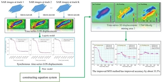
:The previous multi-track InSAR (MTI) method can be used to retrieve mining-induced three-dimensional (3D) surface displacements with high spatial–temporal resolution by incorporating multi-track interferometric synthetic aperture radar (InSAR) observations with a prior model. However, due to the track-by-track strategy used in the previous MTI method, no redundant observations are provided to estimate 3D displacements, causing poor robustness and further degrading the accuracy of the 3D displacement estimation. This study presents an improved MTI method to significantly improve the robustness of the 3D mining displacements derived by the previous MTI method. In this new method, a fused-track strategy, instead of the previous track-by-track one, is proposed to process the multi-track InSAR measurements by introducing a logistic model. In doing so, redundant observations are generated and further incorporated into the prior model to solve 3D displacements. The improved MTI method was tested on the Datong coal mining area, China, with Sentinel-1 InSAR datasets from three tracks. The results show that the 3D mining displacements estimated by the improved MTI method had the same spatial–temporal resolution as those estimated by the previous MTI method and about 33.5% better accuracy. The more accurate 3D displacements retrieved from the improved MTI method can offer better data for scientifically understanding the mechanism of mining deformation and assessing mining-related geohazards.
1. Introduction
Coal is a major component of global fuel supplies worldwide (about 40%) and plays a crucial role in industries such as iron and steel manufacturing [1]. However, underground coal mining can cause ground surface deformation, causing a series of hazards such as landslides and damage to buildings and other infrastructure [2,3,4]. Therefore, it is essential to monitor mining-induced three-dimensional (3D) displacements with high precision and high spatial–temporal resolution for better assessing mining-induced hazards and understanding the mechanism of mining deformation.
Interferometric synthetic aperture radar (InSAR) is a valuable tool for detecting surface deformation induced by underground coal mining over a large area with high spatial resolution [5,6,7,8]. However, InSAR observations are only 1D projections of the true deformation vector onto the radar line-of-sight (LOS) direction [9,10,11]. As a result, the complex pattern of mining deformation in 3D space is difficult to describe well using the InSAR observations of 1D LOS displacements, dramatically narrowing the scope of application of InSAR in mining engineering.
In recent years, a variety of methods have been proposed to retrieve 3D deformation components from InSAR 1D observations [12]. These methods can roughly divided into two categories: (1) fusing multi-track InSAR observations, and (2) incorporating single-track InSAR with prior models [13,14]. Limited by the near-polar orbits of the current SAR sensors, three or more InSAR observations over the same area of interest (AOI) with significantly different imaging geometries cannot be acquired for most areas on Earth [15]. As a consequence, accurate 3D deformation components, especially along the north direction, are difficult to obtain in most cases using the methods that fuse multi-track InSAR observations [12]. With the configuration of the current SAR sensors, the methods of incorporating single-track InSAR observations (which are readily acquired) with prior models have been proven to be a useful alternative for retrieving the 3D deformation components caused by underground coal mining.
However, the methods of incorporating single-track InSAR with prior models have two limitations: (1) the coarse temporal resolution due to the long revisit cycle (e.g., dozens of days) of a single SAR sensor currently, and (2) poor robustness due to the lack of redundant observations for 3D displacement estimation. In 2020, Wang et al. [16] presented a method, referred to as MTI, for enhancing the temporal resolution of 3D mining displacement estimations from multi-track InSAR (MTI) observations. The core idea of the MTI method has the advantage that the multi-track InSAR observations have much denser temporal samples of mining deformation progress (i.e., high temporal resolution) compared with the single-track InSAR. To this end, the MTI method first retrieves 3D mining displacements by incorporating each single-track InSAR observation with the prior model used previously. It then estimates 3D time-series displacements for all the acquisition dates of the collected multi-track SAR images (e.g., several days, depending on the selected SAR images) using a generalized weighting least-squares solver. However, due to the track-by-track processing strategy used in the MTI method, it cannot offer redundant observations for 3D mining displacement estimations. This implies that the poor robustness existing in the previous single-track-based methods still cannot be effectively improved by the MTI method, degrading the accuracy of the calculated 3D time-series displacements caused by underground coal mining (please refer to Section 2.1 for more details).
In this study, an improved MTI method was proposed, with the main aim of improving the poor robustness of the MTI-estimated 3D mining displacements. In this new method, a fused-track strategy, rather than the track-by-track one in the MTI method, was developed to synchronize the multi-track InSAR observations to all the SAR acquisition dates using a logistic model. In doing so, redundant observations will be generated if the synchronized multi-track InSAR measurements are incorporated with the prior model to estimate 3D mining displacements. This strategy would be beneficial for improving the robustness of 3D mining displacement estimations. Theoretically, the improved MTI method can retrieve 3D mining displacements with the same spatial–temporal resolution as those estimated by the previous MTI method, but with better robustness. This superiority has been validated over the Datong coal mining area, China, in this study. The estimated 3D displacements, which have high spatial–temporal resolution and higher accuracy, will be useful for better understanding the deformation mechanism and assessing mining-induced geohazards.
2. Methodology
2.1. Overview of the Track-by-Track MTI Method
The MTI method uses a track-by-track strategy to solve 3D mining displacements by incorporating multi-track InSAR observations with a prior model, called the linear proportional model (LPM). The LPM is defined as the horizontal component of mining-induced surface deformation being linearly proportional to the gradient of its vertical component [14]. For an AOI where SAR images from K multiple tracks have been collected, we can process each track’s SAR images using the time-series InSAR techniques (e.g., the small baseline subset InSAR or the permanent scatterer InSAR) [17,18,19,20,21,22,23,24] to generate multi-track InSAR time-series measurements of LOS displacements.
Let Nk be the number of the kth track’s SAR images acquired on the dates , and let be the corresponding time-series LOS displacements. For an arbitrary pixel over an AOI, the MTI method firstly constructs three independent equations involving mining-induced 3D time-series displacements (denoted as , and in the vertical, easting and northing directions, respectively) on the date () based on the kth track’s InSAR observations from the prior LPM, i.e., [16].
The first equation in System (1) indicates the projection function of the 3D displacement components onto the LOS direction, where , and are the projection vectors, with and being the incidence angle and the heading angle of the selected SAR sensor [25]. The remaining two equations in System (1) are based on the LPM [14], where and represent the gradients of vertical subsidence along the north and east directions, respectively, at a pixel , with RN and RE being the spatial resolutions of the multi-track LOS displacements maps in the north and east directions, respectively; and denote the linear proportional coefficients in the north and east directions, respectively, which are generally considered equal to each other and can be estimated by with b, H and β being the horizontal motion constant, the mining depth and the major influence angle, respectively.
For an AOI with a pixel size of m-by-n, independent equations with a number of 3mn values can be constructed on the basis of Equation (1) for solving the 3D mining displacements (which also number 3mn) of the whole region of interest at the date (refer to [14] for more details). In track-by-track processing (hereafter referred to as the track-by-track strategy), the 3D time-series displacements of the SAR acquisition dates of each track can be obtained. Limited by the revisiting cycles of the current SAR satellites (several to dozens of days), the temporal resolution of the single-track 3D time-series displacements are too coarse to analyze the fast deformation events caused by underground mining. Therefore, the MTI method densifies the temporal resolution of 3D time-series displacements in the vertical, east and north directions using a generalized weighted least-square solver. We take the vertical direction as an example to briefly summarize the key steps. Let be the acquisition date vector of all multi-track SAR images (M in number) in chronological order, and let be the incremental velocities of vertical subsidence in the period of interest. Thus, we can obtain:
where is the coefficient matrix, whose entries are determined by the formation network of the kth track’s small-baseline InSAR pairs [20]; denote the multi-track time-series vertical subsidence solved by Equation (1) and indicates the error term. The incremental velocities are solved using a generalized weighted least-square solver:
where is an interferometric coherence-based weighting matrix (see [16] for more details), and the symbol denotes the Moore–Penrose pseudoinverse operation. Finally, the time-series vertical subsidence at (denoted as ) is obtained by summarizing the incremental subsidence, i.e., by using .
Since the is a union set of all the acquisition dates of the multi-track SAR images, has a much high temporal resolution than any of the single-track time-series vertical subsidence values (i.e., ) (please refer to Wang et al. [16] for more details about the MTI method). However, as can be observed from System (1), no redundant observations are offered to solve the 3D displacements for each track, due to the track-by-track strategy used in the MTI method. This indicates poor robustness to suppress the noise of InSAR observations and the uncertainties of the prior model, degrading the accuracy of the calculated 3D displacements.
2.2. Development of the Improved Fused-Track MTI Method
In the improved MTI method, the multi-track InSAR observations are first aligned (or interpolated) into the same time series (i.e., all acquisition dates of the multi-track SAR images, namely, ) using a logistic model, on a track-by-track basis. In doing so, for an AOI covered by SAR images from K tracks, K multi-track InSAR measurements of LOS time-series displacements can be yielded for an arbitrary date of the collected SAR images (i.e., ). The synchronized multi-track InSAR measurements (K in number) are then incorporated with the LPM so that we can obtain K + 2 equations to solve the 3D time-series displacements. This implies that K − 1 redundant observations (in the case of K ≥ 2) can be provided to suppress the noise of InSAR observations and the uncertainties of the LPM, thus improving the robustness of 3D time-series displacement estimations.
2.2.1. Synchronization of Multi-Track Time-Series LOS Displacements Using the Logistic Model
A key step in the improved MTI method is reliably synchronizing (or interpolating) the asynchronous multi-track InSAR measurements of time-series LOS displacements in the same time series. However, due to the highly nonlinear evolution of mining-induced time-series displacements, it is crucial to select a suitable model for the synchronization. In 2021, Yang et al. [26] found that the temporal evolution of LOS displacements caused by underground longwall mining (a mining method used extensively worldwide) follows an S-shaped growth pattern. The logistic model is a classical S-shaped growth function, where the growth is approximately exponentially in the initial stage, then, as saturation begins, the growth slows to linear and finally stops at maturity [27,28]. Hence, the logistic model was selected to synchronize the multi-track InSAR measurements of the time-series LOS displacements to the acquisition dates of all the multi-track SAR images in this study.
The synchronizing processing method follows. For a highly coherent pixel , the time-series LOS displacements obtained from the kth track’s SAR images, namely, , can be theoretically described by the logistic model, i.e.,
where and denote the parameters of the logistic curve shape, denotes the maximum possible surface deformation at the pixel ; represents the vector of the acquisition dates of the kth track’s SAR images with respect to the reference at the starting time = 0 (i.e.,) and is the error term.
Prior to the synchronizing process, the unknown parameters of the logistic model need to be estimated on a pixel-by-pixel basis. Since Equation (4) is nonlinear, a two-step method is proposed to estimate the unknown parameters of the logistic model in this study. In the first step, a quadratic linearization (QL) of Equation (4) is performed:
At this stage, the parameters of the logistic model can be estimated in a least-square (LS) sense. To reduce the influence of InSAR observation errors on the accuracy of the parameter estimation, we take the LS solution of the parameters as the initial values, then refine the solutions using the Gauss–Newton (GN) method (a common nonlinear inversion method) [29,30]. For the sake of the following argument, the two-step method is referred to as QL+GN. The QL+GN method for model parameter estimation presented here has much better time efficiency and an acceptable accuracy level compared with other evolution searching methods (e.g., the genetic algorithm) used in previous studies [31]. This issue is discussed in detail in Section 4.4.
After the estimation of the parameters of the logistic model in a pixel-by-pixel manner, the asynchronous time-series LOS displacements from the kth track can be interpolated with the multi-track InSAR observations in the same time series (i.e., all multi-track acquisition dates in this study, namely, ) using Equation (4):
where , and denote the parameters estimated by the proposed QL+GN method. At this stage, the synchronized multi-track InSAR measurements of the time-series LOS displacements (denoted as ) on the date are obtained for each high-coherence pixel.
2.2.2. Fused-Track-Based Estimation of 3D Time-Series (TS) Displacements
By performing the logistic model-based synchronization, we can obtain K multi-track InSAR measurements at a high-coherence point . However, it should be pointed out that the K multi-track InSAR observations are usually from the near-polar descending and ascending orbits under the current SAR satellite configuration. This means that it is difficult to accurately solve 3D displacements from the synchronized multi-track InSAR measurements because of the insufficient number of independent imaging geometries (only two). Therefore, the improved MTI method incorporated the synchronized multi-track LOS displacements with the LPM to estimate the 3D time-series displacements associated with underground coal mining.
More specifically, for the pixel at the date , an equation system involving 3D time-series displacements (namely, , and ) can be produced by incorporating the synchronized multi-track LOS displacements with the LPM:
For simplifying the solution of System (7), the last two linear equations are first substituted into the first K equations based on the rule of Gaussian elimination, which generates a system involving only the synchronized multi-track LOS displacements (namely, ) and the unknown subsidence of the mining areas of interest (namely, ), i.e.,
where represents the coefficient matrix, whose entries can be readily deduced from Equation (7). Next, time-series subsidence at the date can be estimated in a weighted least-square sense as
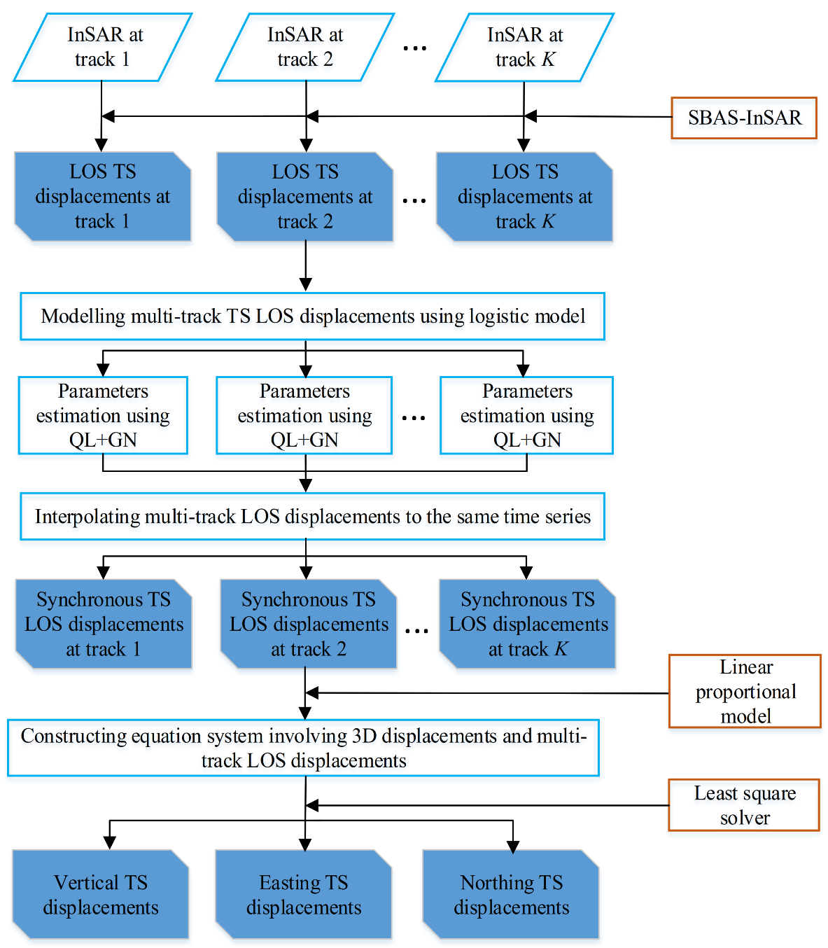
where is the interferometric coherence-based weighting matrix, defined the same as in [16]. Finally, time-series horizontal movements in the east and north directions can be estimated on the basis of the LPM-based constraints (i.e., the last two equations in Equation (7)). The flow chart of the improved MTI method is plotted in Figure 1.
Note that System (7) involves three unknowns (i.e., the 3D time-series displacements at ) and K + 2 equations. This implies that redundant observations can be offered to solve 3D mining displacements if multi-track InSAR observations (K > 1) can be obtained. Consequently, compared with the previous MTI method, where no redundant observations are offered, the improved MTI method proposed in this study can potentially improve the robustness of the estimated 3D displacements (depending on the number of available InSAR datasets and the accuracy of the measured LOS displacements). In addition, it should be pointed out that two assumptions were used for the improved MTI method in the time and space domains. The first is that the time series of LOS displacements associated with underground longwall mining temporally follows the growth of a logistic model. The other is that two-dimensional horizontal movements in the east and north directions at the pixel are linearly proportional to the gradient of subsidence (estimated from the subsidence at the adjacent pixels using the LPM). These two assumptions have both been proven in [26,32], respectively.
3. Experiments and Results
3.1. Study Area and SAR Dataset
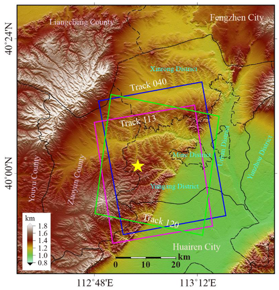
The Datong coalfield was selected to test the improved MTI method. The long-term mining activities in this coalfield have caused a series of geohazards, such as land subsidence and damage to infrastructure [33,34,35]. In this study, 125 Sentinel-1 SAR images were collected over the tested area from January 2018 to May 2019. These SAR images were all acquired in the Terrain Observation by Progressive Scans (TOPS) mode but with two ascending (track 040 and 113) and one descending tracks (track 120). The footprints of these collected SAR images are shown in Figure 2, and the parameters of the collected Sentinel-1 datasets are listed in Table 1.
3.2. Retrieval of Multi-Track Time-Series LOS Displacements
The SBAS-InSAR method [20] was used to process the collected Sentinel-1 SAR images of tracks 040, 113 and 120. The SAR images were first co-registered by the network-based method [36] for each track. We then selected interferometric pairs with the following criteria for making a tradeoff between deformation gradients and redundant observations: (1) a co-registered SAR image was only connected with its two time-adjacent images to form interferometric pairs, and (2) the spatial–temporal baselines of these interferometric pairs were both below the given thresholds (50 days and 300 m in this study). The topographic and flat-earth phase components of each interferometric pair were removed by the SRTM DEM and satellite orbit information. To achieve a resolution of 20 m in both the range and azimuth direction, we applied a multi-looking factor of 5:1 (range, azimuth) for generating the interferograms. The Goldstein filter was exploited to reduce the phase noise in the differential interferograms [37,38], and the filtered differential interferograms were unwrapped using the network programming-based phase unwrapping method [39]. Subsequently, singular value decomposition (SVD (in the case of the rank-deficient problem) or the least-square solver (for an over-conditioned case) was used to derive the time-series LOS displacements in a track-by-track manner. Finally, the time-series LOS displacements, starting from zero with respect to the date of the earliest image, were geocoded and resampled to a common map projection grid for the subsequent 3D displacement retrieval.
In this study, we selected an AOI (marked by the yellow star in Figure 2) to test the reliability of the improved MTI method. The reasons for selecting the AOI are twofold. First, visually obvious deformation occurred in the AOI during the time period of interest (i.e., from January 2018 to May 2019) due to underground coal mining in the Datong coalfield (see Figure 3 for the geocoded cumulative multi-track LOS displacements). Second, nearly real-time 3D displacement measurements obtained by a continuous GPS receiver in the AOI (the location is marked by red triangle in Figure 3) were available to validate the feasibility and the reliability of the improved MTI method.
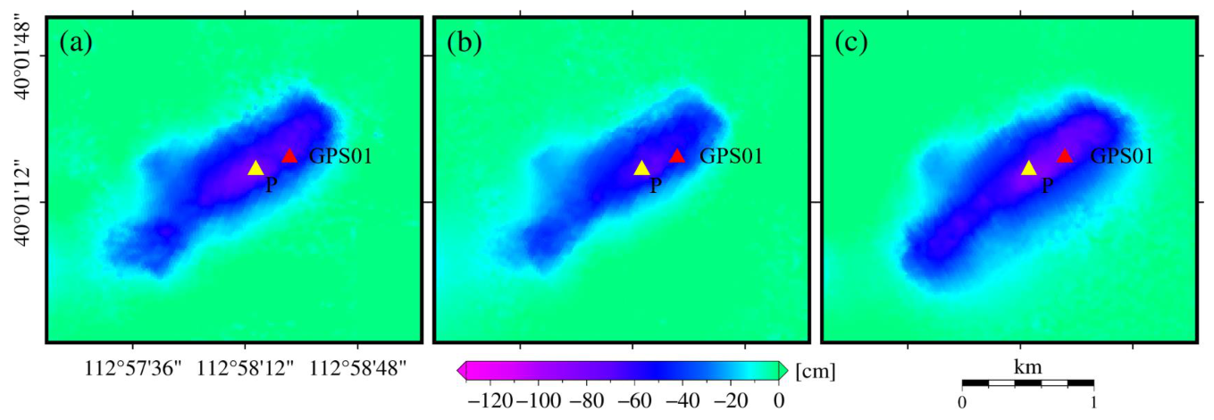
As is shown in Figure 3, different spatial patterns were present in the generated multi-track cumulative LOS displacements maps associated with the same mining operation, due to the different SAR imaging geometries. In addition, maximum LOS displacements of about 78, 71 and 89 cm were measured for the track 040, 113 and 120 InSAR datasets, respectively. The different deformation patterns presented in Figure 3 would hinder the interpretation of deformation events and assessment of the resulting geohazards. This fact suggests that it is essential to decompose the 3D displacement components of InSAR-measured LOS displacements.
3.3. Synchronization of the Multi-Track Time-Series LOS Displacements
The logistic model was used to synchronize the multi-track InSAR measurements of the time-series LOS displacements. For this, the unknown parameters of the logistic model were estimated using the proposed QL+GN algorithm in a pixel-by-pixel manner (see Section 2.2.1). The estimated model parameters (a, b and c) of tracks 040, 113 and 120 are plotted in Figure 4. Note that the time-series LOS displacements over the areas where underground mining had an insignificant influence on should be negligible and should theoretically not follow an S-shaped growth curve. As a result, a linear model, instead of the logistic model, was chosen to synchronize the multi-track InSAR measurements of time-series LOS displacements. Having obtained the parameters of the logistic model, the multi-track InSAR observations of the LOS displacements were interpolated to the same time series (i.e., all acquisition dates of the multi-track SAR images collected in this study) to generate synchronous time-series LOS displacements.
3.4. Estimation of Mining-Induced Time-Series 3D Displacements
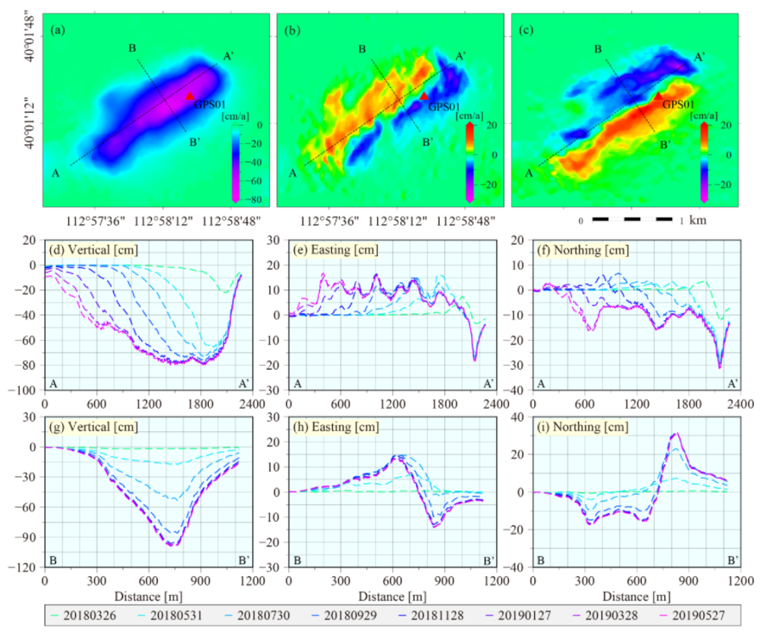
Prior to estimating the kinematic 3D mining displacements, an inverse distance interpolation was performed for the sake of the following estimation of 3D mining displacements. The improved MTI method was then used to generate the time-series 3D displacements, starting from zero with respect to the date of the earliest image, based on the synchronized multi-track LOS displacements. Here, the prior parameters of the LPM, i.e., the horizontal movement constant b, the mining depth H and the tangent of the major influence angle tanβ, were given as b = 0.31, H = 480 m and tanβ = 1.8, respectively. Figure 5a–c shows the annual rates of the estimated time-series 3D displacements from January 2018 to May 2019. As seen in this figure, the maximum displacement rates over the region of interest between January 2018 and May 2019 were around −80 cm, 20 cm and 23 cm per year, in the vertical, easting and northing directions, respectively. Figure 5d–i plots the estimated time-series 3D displacements along the profiles AA′ and BB′ due to underground coal mining for demonstrating the evolution of 3D displacement.
3.5. Accuracy Evaluation
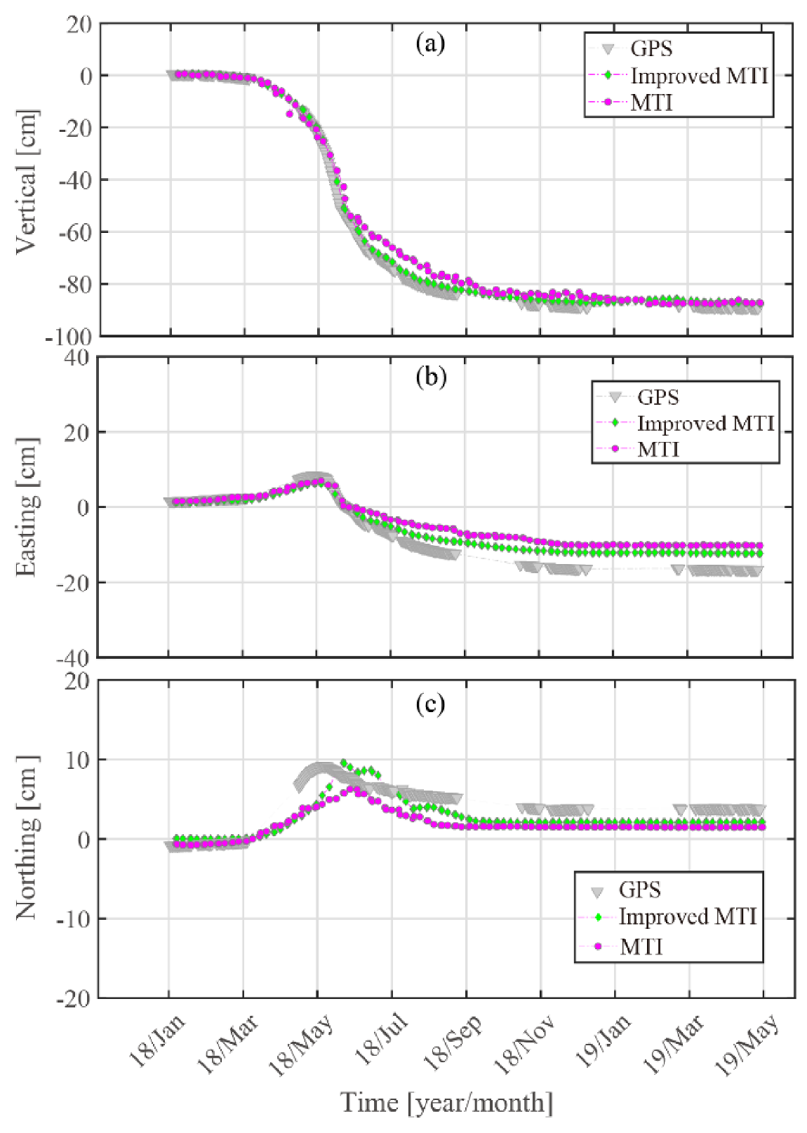
The in situ 3D displacements measured by a continuous GPS receiver (named GPS01, marked by the red triangle in Figure 5a–c) were used to validate the accuracy of the 3D displacements calculated by the improved MTI method. The kinematic 3D displacements derived by the proposed improved MTI method and the MTI method are plotted together with the GPS-derived 3D displacements for point GPS01 in Figure 6a–c. Note that, due to the missing GPS signals, in situ 3D displacements for parts of the time period (e.g., from 9 September 2018 to 4 November 2018) between January 2018 and May 2019 are unavailable.
As can be seen from Figure 6, the time-series 3D displacements estimated by the improved MTI method (green diamonds) agree well with the in situ GPS measurements (gray triangles) from the GPS01 receiver, with root mean square errors (RMSEs) of 1.4, 2.8 and 1.7 cm in the vertical, easting and northing directions, respectively. These RMSEs occupy 1.6%, 22.7% and 17.7% of the maximum 3D displacements (i.e., −87.55, −12.32 and 9.58 cm) in the vertical, easting and northing directions, respectively. Besides the uncertainty of the theoretical LPM, the errors of the InSAR-derived LOS displacements, particularly those due to unwrapping errors and decorrelation noise, are the major source of error in the solved 3D time-series displacements using the improved MTI method. As suggested by Yang et al. [13], the uncertainties of the LPM and InSAR observations would cause larger errors in the calculated horizontal movements in the easting and northing directions, compared with those in the vertical direction. This can also be observed in Figure 6, where a larger relative bias to the maximum displacement occurs in the calculated easting and northing movements compared with those in the vertical direction.
4. Discussion
4.1. Comparison of the Robustness of the Improved MTI and MTI Methods
4.1.1. Simulation Analysis
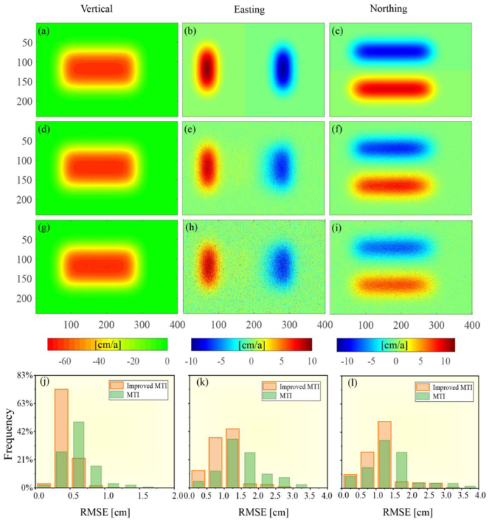
The robustness of the improved MTI and MTI methods was first analyzed with simulation data. More specifically, we first simulated time-series 3D displacements caused by underground mining at nine time periods using the probability integration method (a deformation model widely used in mining engineering) [13,40,41]. Figure 7a–c shows the annual rates of the simulated 3D displacements in the vertical, easting and northing directions, respectively. The simulated time-series 3D displacements were then projected onto the LOS directions by following the same imaging geometries listed in Table 1. Next, Gaussian noise with a mean of zero and a standard deviation (STD) of 0.8, 0.65, and 0.9 cm was added to the projected time-series LOS displacements of three tracks, respectively. Finally, the time-series 3D displacements in the vertical, easting and northing directions were estimated from the projected LOS displacements with Gaussian noise by using the improved MTI and the previous MTI methods.
Figure 7 shows a comparison of the annual rates of the 3D displacements estimated by the improved MTI (d–f) and MTI (g–i) methods. As shown in this visualization, the 3D displacements estimated by the improved MTI methods are less noisy (more accurate), especially in the horizontal direction, than those estimated by the MTI method. In addition, the mean RMSEs of the improved MTI-estimated 3D displacements are about 0.5, 1.2 and 1.0 cm, respectively, in the vertical, easting and northing directions. This result indicates an improvement of around 40%, 50% and 70% with respect to the RMSEs of the MTI-estimated 3D displacements (i.e., 0.7, 1.8 and 1.7 cm, respectively) (see Figure 7j–l). The results suggest that the improved MTI method can significantly improve the robustness of 3D displacement estimation (with a mean of 53% in this simulated case) compared with the previous MTI method.
4.1.2. Real Data Analysis
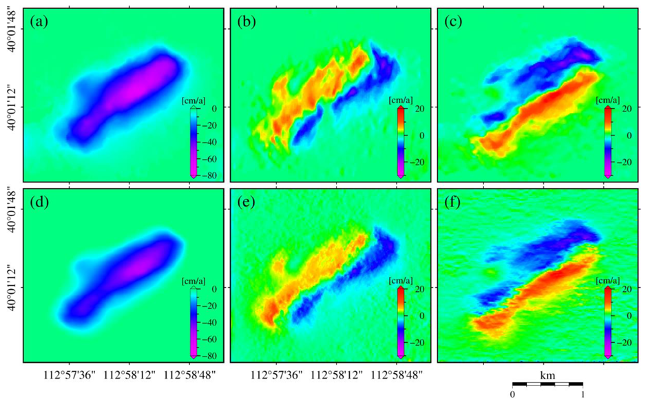
The real data described in Section 3.1 were used to further analyze the robustness of the improved MTI and MTI methods (a comparison of the annual rate maps of the 3D displacements estimated by these two methods is shown in Appendix A, Figure A1). Figure 6 shows a comparison of the time-series 3D displacements estimated by these two methods with the in situ 3D displacements at the point of the GPS01 receiver. Table 2 lists the RMSEs of the 3D displacements estimated by these two methods.
As can be seen from Figure 6 and Table 2, the 3D displacements estimated by the improved MTI method have a better agreement with the in situ measurements than the 3D displacements derived by the MTI method. The RMSEs of the 3D displacements resolved by the improved MTI method are 1.4, 2.8 and 1.7 cm, respectively, in the vertical, easting and northing directions. These RMSEs indicate an improvement in accuracy of about 39.1%, 20.0% and 41.4% (with a mean improvement of 33.5%) compared with the MTI-estimated 3D displacements (i.e., 2.3, 3.5 and 2.9 cm). The comparison suggests that the improved MTI method has better robustness than the MTI method, owing to the generation of redundant LOS observations.
4.2. Capability of the Logistic Model for Modeling Mining-Induced LOS Displacements
Theoretically, the improvement in the robustness of the improved MTI method primarily depends on the number and accuracy of the redundant LOS observations generated. For an AOI, the track number of the collected multi-track InSAR datasets is constant. Thus, the accuracy of the generated redundant LOS observations is essential for improving the robustness of the estimated 3D mining displacements. In the improved MTI method, redundant observations are generated by interpolating the multi-track measurements of LOS displacements using the logistic model. Thus, the capability of the selected logistic model for modeling the temporal evolution of mining-induced LOS displacements plays an important role in the improved MTI method. This issue will be discussed in detail in this section.
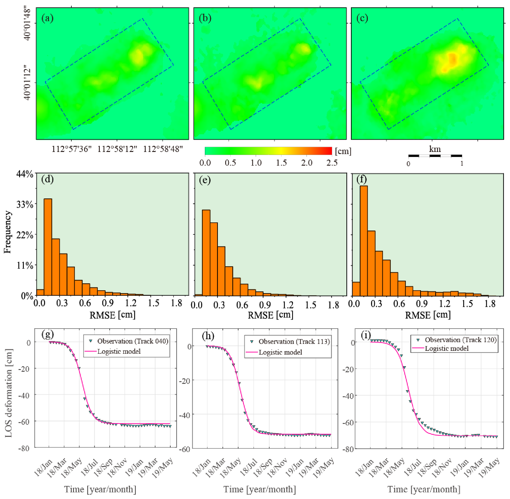
Figure 8a–f shows the fitting RMSEs and the corresponding histograms of the time-series LOS displacements for tracks 040, 113 and 120 from the logistic model. As can be seen, the RMSEs range from 0 to 1.9 cm, with mean RMSEs of 0.3, 0.3 and 0.4 cm for tracks 040, 113 and 120, respectively. In addition, as observed in Figure 8d–f, the RMSEs in the range of 0 to 1 cm occupy 98%, 99% and 95% of all pixels for tracks 040, 113 and 120, respectively. Figure 8g–i plots an example of the multi-track LOS displacement fitting at the GPS01 point using the logistic model, which also demonstrates a small misfit between the InSAR-measured and the logistic-fitted LOS displacements. These results indicate that the selected logistic model in this study can describe the temporal evolution of LOS displacements caused by underground longwall mining. As a consequence, the synchronous multi-track observations of LOS displacements with an acceptable accuracy level (i.e., interpolation RMSEs of 0.91, 0.65 and 1.50 cm for tracks 040, 113 and 120 at the GPS01 point) could theoretically be interpolated using the logistic model.
4.3. Selection of the Models to Interpolate Multi-Track LOS Displacements
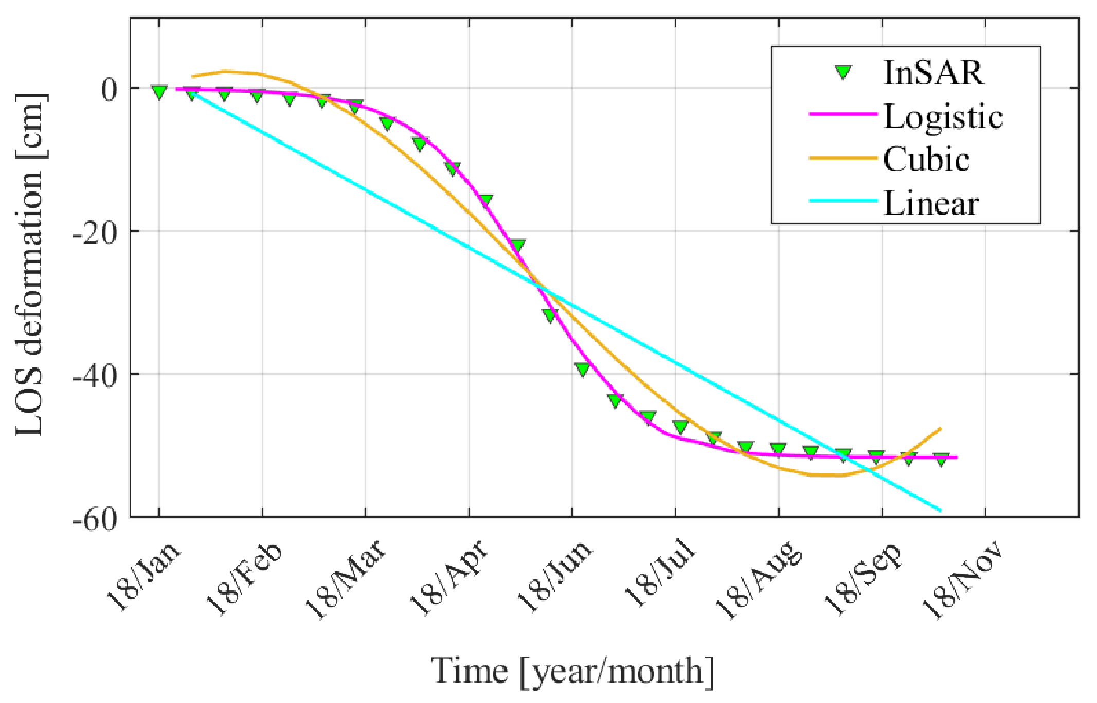
As stated previously, the capability of the selected models to describe the temporal evolution of the mining-induced LOS displacements has a significant influence on the robustness of the 3D displacements estimated by the improved MTI method. In this study, the logistic model (a common S-shaped growth function) was selected and its capability was tested in Section 4.2. To show the importance of the selected model for improving the robustness of the 3D displacements, we first took the multi-track InSAR observations from track 113 at the point of the GPS01 receiver as an example. Two common mathematical models (i.e., linear and cubic polynomials) [20,42,43] that are widely used in the retrieval of InSAR time-series displacements were then selected as alternatives to demonstrate the fitting performance of the multi-track InSAR observations (see Figure 9).
As can be seen from Figure 9, due to the highly nonlinear evolution, the linear function had difficulty reliably describing the mining-induced LOS displacements (with a fitting RMSE of 6.7 cm). Compared with the linear function, the fitting RMSE of the cubic polynomial (i.e., 3.2 cm) was smaller than that of the linear function, whereas it was much larger (about fivefold) than the fitting RMSE of the logistic model at the GPS01 point (i.e., 0.6 cm). This result indicates that, with respect to the two common models used in the InSAR community (i.e., linear and cubic polynomials), the logistic model is more suitable to use for interpolating the multi-track LOS displacements into the same time series. Note that besides the logistic model, other functions of the sigmoid growth function family (e.g., the Weibull and Gompertz models) [44] could theoretically be selected to describe the S-shaped growth pattern of the time-series LOS displacements caused by underground longwall mining.
4.4. Efficiency of the QL+GN Algorithm for Estimating the Parameters of the Logistic Model
Accurate estimation of the parameters of the selected logistic model is a key step for ensuring the accuracy of the synchronized multi-track InSAR observations of LOS displacements, besides the model errors. In fact, some nonlinear searching methods have been proposed to estimate the parameters of the logistic model. For instance, the hybrid genetic algorithm (GA) with simulated annealing (SA) (referred to as GA+SA), which generates the initial values of the parameter using the GA and then refines them with the SA, has been proven to be an effective algorithm for estimating the parameters of the logistic model, since it generally has a high accuracy level without designating the initial parameters [16,31]. However, the GA+SA algorithm has poor efficiency in terms of computation time. To this end, we proposed the QL+GN algorithm (see Section 2.2.1) for keeping the same high accuracy level but dramatically reducing the time cost of parameter estimation.
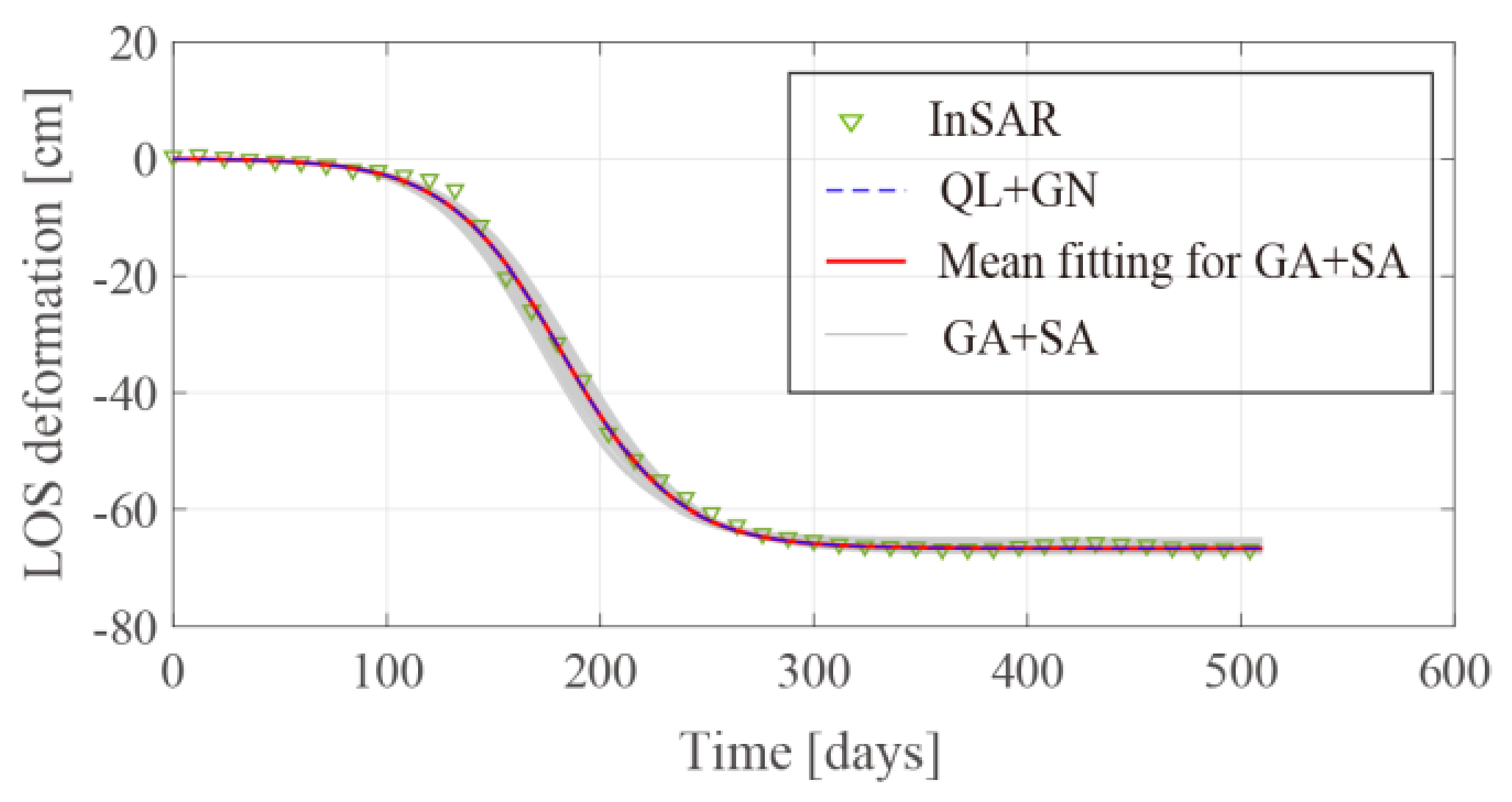
To validate the efficiency of the QL+GN algorithm, a comparison of the parameters estimated using the QL+GN and GA+SA algorithms is presented in this section. For this, the population size, crossover fraction and maximum generation of GA +SA were 100, 0.65 and 700, respectively [31]. Figure 10 shows a comparison of the fit of the InSAR observations for track 113 at the mining center (the yellow triangle in Figure 3) as an example. Inversion of the logistic model parameters was carried out independently 50 times using the GA+SA and QL+GN algorithms for reducing the random errors. Table 3 lists the means of the GA+SA and QL+GN inverted parameters of the logistic model (namely, a, b and c). In addition, the mean computation costs of model parameter estimation using these two methods are listed in Table 3 for comparison.
It can be observed from Figure 10 that the random operations in the GA had a significant influence on the fit of the LOS displacements for the 50 iterations (marked by gray curves), although the SA was used to re-estimate the model parameters in the GA+SA algorithm. However, the mean fit using the GA+SA algorithm shows good agreement with the InSAR-measured LOS displacements (marked by red curve), with a RMSE of 0.62 cm. Concerning the proposed QL+GN algorithm, the random influence on the logistic fitting that occurred with the GA+SA reduced dramatically for the 50 parameter estimations (almost complete overlap). In addition, the mean fit using the QL+GN algorithm agrees well the InSAR observations, with a RMSE of 0.61 cm. This result suggests that the QL+GN algorithm shows nearly the same accuracy level for estimating the parameters of the logistic model (see Table 3) as the previous GA+SA algorithm. In addition, Table 3 also shows that the mean computation cost of the parameter inversion of the logistic model using the GA+SA algorithm (2.1 s for a pixel in this case) was much longer (21 times) than that of the proposed QL+GN algorithm (0.1 in this case). The dramatic reduction in time cost is beneficial for the retrieval of 3D time-series displacements using the improved MTI method, especially over a large area (e.g., one with millions of pixels). These results suggest that the proposed QL+GN algorithm is capable of estimating the parameters of the logistic model with the same accuracy as the GA+SA algorithm, but with less randomness and a much shorter computation time.
5. Conclusions
This paper presents an improved MTI method for retrieving the more robust 3D time-series displacements associated with underground coal mining obtained from multi-track InSAR observations, compared with the previous MTI method. To this end, the logistic model was first used to interpolate the asynchronous multi-track InSAR measurements. An algorithm (QL+GN) was presented to estimate the parameters of the logistic model, which had nearly the same accuracy level as the previous algorithms (e.g., GA+SA) but with much higher time cost efficiency (1/21 in this study). Next, the interpolated (or synchronous) multi-track InSAR observations were incorporated with the LPM to solve mining-induced 3D displacements. Owing to the generation of redundant observations using the logistic model, the improved MTI method had better robustness than the previous MTI method (in which no redundant observations are offered). This assumption was tested by simulation and real datasets from the Datong coalfield in China. The results suggest that, with respect to the previous MTI method, the improved MTI method can more robustly retrieve 3D time-series displacements with the same high spatial-temporal resolution (e.g., with an improvement in accuracy of 53% and 33.5% for the simulation and the real data, respectively). These 3D kinematic displacements with a higher accuracy level and high spatial-temporal resolution will have a wider scope of application in mining engineering (e.g., a better understanding of the mechanism of mining deformation and assessing mining-related geohazards).
Author Contributions
Conceptualization, Z.Y.; funding acquisition, L.W.; investigation, J.S.; methodology, J.S. and Z.Y.; supervision, Z.Y. and L.W.; validation, J.S. and S.Q.; visualization, S.Q.; writing—original draft, J.S.; writing—review and editing, Z.Y. and L.W. All authors have read and agreed to the published version of the manuscript.
Funding
This work was partly supported by the Basic Science Center of the National Natural Science Foundation of China (Grant No. 72088101); the National Natural Science Foundation of China (Grant No. 41904005); the Natural Science Foundation of Hunan Province, China (Grant No. 2020JJ4699); the Innovation Leading Program of Central South University (Grant No. 2018RS3013); the Natural Science Foundation of Hunan Province, China (Grant No. 2020JJ4699); and the Research Foundation of Education Bureau of Hunan Province, China (Grant No. 20K134).
Institutional Review Board Statement
Not applicable.
Informed Consent Statement
Not applicable.
Data Availability Statement
The Sentinel-1 data presented in this study are openly available in ESA/Copernicus at https://scihub.copernicus.eu (accessed on 17 July 2021). The SRTM data presented in this study are openly available in the National Aeronautics and Space Administration (NASA, United States).
Acknowledgments
The authors gratefully acknowledge the Sentinel-1 data provided by ESA/Copernicus, and the SRTM data provided by the National Aeronautics and Space Administration (NASA, United States).
Conflicts of Interest
The authors declare no conflict of interest.
Appendix A
Figure A1.
Annual average 3D deformation rates estimated by proposed new method and the MTI-based method. (a–c) The average deformation rates in the vertical, easting and northing directions, respectively, derived by the proposed method. (d–f) The results derived by the MTI-based method.
Figure A1.
Annual average 3D deformation rates estimated by proposed new method and the MTI-based method. (a–c) The average deformation rates in the vertical, easting and northing directions, respectively, derived by the proposed method. (d–f) The results derived by the MTI-based method.

References
- IEA. Coal 2019; International Energy Agency: Paris, France, 2019. [Google Scholar]
- Cando Jacome, M.; Martinez-Grana, A.M.; Valdes, V. Detection of Terrain Deformations Using InSAR Techniques in Relation to Results on Terrain Subsidence (Ciudad de Zaruma, Ecuador). Remote Sens. 2020, 12, 1598. [Google Scholar] [CrossRef]
- Vu Khac, D.; Thanh Dong, N.; Ngoc Hung, D.; Thi Loi, D.; Xuan Vinh, D.; Weber, C. Land subsidence induced by underground coal mining at Quang Ninh, Vietnam: Persistent scatterer interferometric synthetic aperture radar observation using Sentinel-1 data. Int. J. Remote Sens. 2021, 42, 3563–3582. [Google Scholar] [CrossRef]
- Diao, X.P.; Bai, Z.H.; Wu, K.; Zhou, D.W.; Li, Z.L. Assessment of mining-induced damage to structures using InSAR time series analysis: A case study of Jiulong Mine, China. Environ. Earth Sci. 2018, 77, 166. [Google Scholar] [CrossRef]
- Bateson, L.; Cigna, F.; Boon, D.; Sowter, A. The application of the Intermittent SBAS (ISBAS) InSAR method to the South Wales Coalfield, UK. Int. J. Appl. Earth Obs. Geoinf. 2015, 34, 249–257. [Google Scholar] [CrossRef] [Green Version]
- Gee, D.; Bateson, L.; Sowter, A.; Grebby, S.; Novellino, A.; Cigna, F.; Marsh, S.; Banton, C.; Wyatt, L. Ground Motion in Areas of Abandoned Mining: Application of the Intermittent SBAS (ISBAS) to the Northumberland and Durham Coalfield, UK. Geosciences 2017, 7, 85. [Google Scholar] [CrossRef] [Green Version]
- Milczarek, W.; Kopec, A.; Glabicki, D.; Bugajska, N. Induced Seismic Events-Distribution of Ground Surface Displacements Based on InSAR Methods and Mogi and Yang Models. Remote Sens. 2021, 13, 1451. [Google Scholar] [CrossRef]
- Malinowska, A.A.; Witkowski, W.T.; Hejmanowski, R.; Chang, L.; van Leijen, F.J.; Hanssen, R.F. Sinkhole occurrence monitoring over shallow abandoned coal mines with satellite-based persistent scatterer interferometry. Eng. Geol. 2019, 262, 105336. [Google Scholar] [CrossRef]
- Ren, H.; Feng, X. Calculating vertical deformation using a single InSAR pair based on singular value decomposition in mining areas. Int. J. Appl. Earth Obs. Geoinf. 2020, 92, 102115. [Google Scholar] [CrossRef]
- Fan, H.; Wang, L.; Wen, B.; Du, S. A New Model for three-dimensional Deformation Extraction with Single-track InSAR Based on Mining Subsidence Characteristics. Int. J. Appl. Earth Obs. Geoinf. 2021, 94, 102223. [Google Scholar] [CrossRef]
- Zheng, M.; Deng, K.; Fan, H.; Huang, J. Monitoring and analysis of mining 3D deformation by multi-platform SAR images with the probability integral method. Front. Earth Sci. 2019, 13, 169–179. [Google Scholar] [CrossRef]
- Yang, Z.; Li, Z.; Zhu, J.; Wang, Y.; Wu, L. Use of SAR/InSAR in Mining Deformation Monitoring, Parameter Inversion, and Forward Predictions: A Review. IEEE Geosci. Remote Sens. Mag. 2020, 8, 71–90. [Google Scholar] [CrossRef]
- Yang, Z.; Li, Z.; Zhu, J.; Feng, G.; Wang, Q.; Hu, J.; Wang, C. Deriving time-series three-dimensional displacements of mining areas from a single-geometry InSAR dataset. J. Geod. 2018, 92, 529–544. [Google Scholar] [CrossRef]
- Li, Z.W.; Yang, Z.F.; Zhu, J.J.; Hu, J.; Wang, Y.J.; Li, P.X.; Chen, G.L. Retrieving three-dimensional displacement fields of mining areas from a single InSAR pair. J. Geod. 2015, 89, 17–32. [Google Scholar] [CrossRef]
- Hu, J.; Li, Z.; Ding, X.; Zhu, J.; Zhang, L.; Sun, Q. Resolving three-dimensional surface displacements from InSAR measurements: A review. Earth-Sci. Rev. 2014, 133, 1–17. [Google Scholar] [CrossRef]
- Wang, Y.; Yang, Z.; Li, Z.; Zhu, J.; Wu, L. Fusing adjacent-track InSAR datasets to densify the temporal resolution of time-series 3-D displacement estimation over mining areas with a prior deformation model and a generalized weighting least-squares method. J. Geod. 2020, 94, 47. [Google Scholar] [CrossRef]
- Osmanoğlu, B.; Sunar, F.; Wdowinski, S.; Cabral-Cano, E. Time series analysis of InSAR data: Methods and trends. ISPRS J. Photogramm. Remote Sens. 2016, 115, 90–102. [Google Scholar] [CrossRef]
- Lanari, R.; Lundgren, P.; Manzo, M.; Casu, F. Satellite radar interferometry time series analysis of surface deformation for Los Angeles, California. Geophys. Res. Lett. 2004, 31, L23613. [Google Scholar] [CrossRef]
- Hooper, A.; Bekaert, D.; Spaans, K.; Arikan, M. Recent advances in SAR interferometry time series analysis for measuring crustal deformation. Tectonophysics 2012, 514, 1–13. [Google Scholar] [CrossRef]
- Berardino, P.; Fornaro, G.; Lanari, R.; Sansosti, E. A new algorithm for surface deformation monitoring based on small baseline differential SAR interferograms. IEEE Trans. Geosci. Remote Sens. 2002, 40, 2375–2383. [Google Scholar] [CrossRef] [Green Version]
- Ferretti, A.; Prati, C.; Rocca, F. Permanent scatterers in SAR interferometry. IEEE Trans. Geosci. Remote Sens. 2001, 39, 8–20. [Google Scholar] [CrossRef]
- Hooper, A.; Segall, P.; Zebker, H. Persistent scatterer interferometric synthetic aperture radar for crustal deformation analysis, with application to Volcan Alcedo, Galapagos. J. Geophys. Res.-Solid Earth 2007, 112, B07407. [Google Scholar] [CrossRef] [Green Version]
- Sousa, J.J.; Ruiz, A.M.; Hanssen, R.F.; Bastos, L.; Gil, A.J.; Galindo-Zaldivar, J.; de Galdeano, C.S. PS-InSAR processing methodologies in the detection of field surface deformation Study of the Granada basin (Central Betic Cordilleras, southern Spain). J. Geodyn. 2010, 49, 181–189. [Google Scholar] [CrossRef]
- Tizzani, P.; Berardino, P.; Casu, F.; Euillades, P.; Manzo, M.; Ricciardi, G.P.; Zeni, G.; Lanari, R. Surface deformation of Long Valley Caldera and Mono Basin, California, investigated with the SBAS-InSAR approach. Remote Sens. Environ. 2007, 108, 277–289. [Google Scholar] [CrossRef]
- Fialko, Y.; Simons, M.; Agnew, D. The complete (3-D) surface displacement field in the epicentral area of the 1999 Mw7. 1 Hector Mine earthquake, California, from space geodetic observations. Geophys. Res. Lett. 2001, 28, 3063–3066. [Google Scholar] [CrossRef] [Green Version]
- Yang, Z.; Xu, B.; Li, Z.; Wu, L.; Zhu, J. Prediction of Mining-Induced Kinematic 3-D Displacements From InSAR Using a Weibull Model and a Kalman Filter. IEEE Trans. Geosci. Remote Sens. 2021, 1, 1–12. [Google Scholar] [CrossRef]
- Kratzsch, I.H. Mining Subsidence Engineering; Environmental Geology and Water Sciences: New York, NY, USA, 1983. [Google Scholar]
- Zhang, W.Z.; Zou, Y.F.; Ren, X.F. Research on logistic model in forecasting subsidence single-point during mining. J. Min. Saf. Eng. 2009, 26, 486–489. [Google Scholar]
- Mao, W.-L.; Ma, W.-J.; Chien, Y.-R.; Ku, C.-H. New Adaptive All-pass Based Notch Filter for Narrowband/FM Anti-jamming GPS Receivers. Circuits Syst. Signal Process. 2011, 30, 527–542. [Google Scholar] [CrossRef]
- Worthen, J.; Stadler, G.; Petra, N.; Gurnis, M.; Ghattas, O. Towards adjoint-based inversion for rheological parameters in nonlinear viscous mantle flow. Phys. Earth Planet. Inter. 2014, 234, 23–34. [Google Scholar] [CrossRef]
- Yang, Z.; Li, Z.; Zhu, J.; Yi, H.; Hu, J.; Feng, G. Deriving Dynamic Subsidence of Coal Mining Areas Using InSAR and Logistic Model. Remote Sens. 2017, 9, 125. [Google Scholar] [CrossRef] [Green Version]
- Peng, S.S. Surface Subsidence Engineering: Theory and Practice; CSIRO Publishing: Clayton, VIC, Australia, 2020. [Google Scholar]
- Yang, C.; Lu, Z.; Zhang, Q.; Liu, R.; Ji, L.; Zhao, C. Ground deformation and fissure activity in Datong basin, China 2007-2010 revealed by multi-track InSAR. Geomat. Nat. Hazards Risk 2019, 10, 465–482. [Google Scholar] [CrossRef]
- Zhao, C.; Lu, Z.; Zhang, Q.; Yang, C.; Zhu, W. Mining collapse monitoring with SAR imagery data: A case study of Datong mine, China. J. Appl. Remote Sens. 2014, 8, 083574. [Google Scholar] [CrossRef]
- Zhi-ying, H. Movement law of coal mining subsidence surface ground in Datong Mining Area. Coal Sci. Technol. 2004, 2, 50–52. [Google Scholar] [CrossRef]
- Xu, B.; Li, Z.; Zhu, Y.; Shi, J.; Feng, G. Kinematic Coregistration of Sentinel-1 TOPSAR Images Based on Sequential Least Squares Adjustment. IEEE J. Sel. Top. Appl. Earth Obs. Remote Sens. 2020, 13, 3083–3093. [Google Scholar] [CrossRef]
- Goldstein, R.M.; Werner, C.L. Radar interferogram filtering for geophysical applications. Geophys. Res. Lett. 1998, 25, 4035–4038. [Google Scholar] [CrossRef] [Green Version]
- Fu, P.; Ge, Y.; Ma, C.; Jia, X.; Shan, X.; Li, F.; Zhang, X. A Study of Land Subsidence by Radar Remote Sensing at Datong Jurassic & Carboniferous Period Coalfield. In Proceedings of the 2009 2nd International Congress on Image and Signal Processing, Tianjin, China, 17–19 October 2009; Volume 942, pp. 1–4. [Google Scholar] [CrossRef]
- Costantini, M. A novel phase unwrapping method based on network programming. IEEE Trans. Geosci. Remote Sens. 1998, 36, 813–821. [Google Scholar] [CrossRef]
- Diao, X.; Wu, K.; Hu, D.; Li, L.; Zhou, D. Combining differential SAR interferometry and the probability integral method for three-dimensional deformation monitoring of mining areas. Int. J. Remote Sens. 2016, 37, 5196–5212. [Google Scholar] [CrossRef]
- Yang, Z.F.; Li, Z.W.; Zhu, J.J.; Hu, J.; Wang, Y.J.; Chen, G.L. InSAR-Based Model Parameter Estimation of Probability Integral Method and Its Application for Predicting Mining-Induced Horizontal and Vertical Displacements. IEEE Trans. Geosci. Remote Sens. 2016, 54, 4818–4832. [Google Scholar] [CrossRef]
- Hanssen, R.; Bamler, R. Evaluation of interpolation kernels for SAR interferometry. IEEE Trans. Geosci. Remote Sens. 1999, 37, 318–321. [Google Scholar] [CrossRef]
- Ronchin, E.; Masterlark, T.; Dawson, J.; Saunders, S.; Molist, J.M. Imaging the complex geometry of a magma reservoir using FEM-based linear inverse modeling of InSAR data: Application to Rabaul Caldera, Papua New Guinea. Geophys. J. Int. 2017, 209, 1746–1760. [Google Scholar] [CrossRef] [Green Version]
- Zeide, B. Analysis of growth equations. For. Sci. 1993, 39, 594–616. [Google Scholar] [CrossRef]
Figure 1.
Flow chart of the improved MTI method for retrieving time-series 3D mining displacements. TS, time-series.
Figure 1.
Flow chart of the improved MTI method for retrieving time-series 3D mining displacements. TS, time-series.

Figure 2.
Geographic location of the region of interest (marked by the yellow star) and the footprints of the collected Sentinel-1 SAR images.
Figure 2.
Geographic location of the region of interest (marked by the yellow star) and the footprints of the collected Sentinel-1 SAR images.

Figure 3.
Cumulative LOS displacements over the AOI (marked by the yellow star in Figure 2) from (a) track 040, (b) track 113 and (c) track 120 Sentinel-1 SAR images in the period from January 2018 to May 2019. The red triangle represents the location of a continuously deployed GPS receiver named GPS01. The yellow triangle shows a point P near the mining center of the AOI.

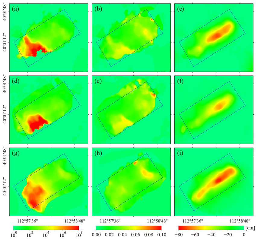
Figure 4.
The QL+GN-estimated parameters a (a,d,g), b (b,e,h) and c (c,f,i) of the logistic model for tracks 040 (a–c), 113 (d–f) and 120 (g–i). The blue dashed rectangular boxes represent the area of deformation due to underground mining. Note that the parameters a (a,d,g) have no units, and the units of b (b,e,h) are the reciprocal of the time units.

Figure 5.
(a–c) Estimated annual rates of 3D displacement over the AOI between January 2018 and May 2019 in the vertical, easting and northing directions, respectively. (d–i) The estimated time-series 3D displacements along the profiles AA′ and BB′ (marked by dashed lines in (a–c)).
Figure 5.
(a–c) Estimated annual rates of 3D displacement over the AOI between January 2018 and May 2019 in the vertical, easting and northing directions, respectively. (d–i) The estimated time-series 3D displacements along the profiles AA′ and BB′ (marked by dashed lines in (a–c)).

Figure 6.
(a–c) Comparison of the improved MTI method results and the original MTI method for surface point GPS01 (marked by the red triangle in Figure 3) in the region of interest between January 2018 and May 2019.
Figure 6.
(a–c) Comparison of the improved MTI method results and the original MTI method for surface point GPS01 (marked by the red triangle in Figure 3) in the region of interest between January 2018 and May 2019.

Figure 7.
The average 3D displacements rates in the vertical, easting and northing directions generated by the simulation procedure (a–c), the improved MTI method (d–f) and the MTI (g–i) methods. (j–l) Three-dimensional RMSE statistical histograms.
Figure 7.
The average 3D displacements rates in the vertical, easting and northing directions generated by the simulation procedure (a–c), the improved MTI method (d–f) and the MTI (g–i) methods. (j–l) Three-dimensional RMSE statistical histograms.

Figure 8.
Fitting RMSEs (a–c) and the corresponding histograms (d–f) of the time-series LOS displacements for tracks 040, 113 and 120 using the logistic model. (g–i) An example of the fit of the time-series LOS displacements at the GPS01 point using the logistic model.
Figure 8.
Fitting RMSEs (a–c) and the corresponding histograms (d–f) of the time-series LOS displacements for tracks 040, 113 and 120 using the logistic model. (g–i) An example of the fit of the time-series LOS displacements at the GPS01 point using the logistic model.

Figure 9.
Comparison of the time-series LOS displacement fitting for track 113 at the GPS01 point using logistic, linear and cubic polynomials.
Figure 9.
Comparison of the time-series LOS displacement fitting for track 113 at the GPS01 point using logistic, linear and cubic polynomials.

Figure 10.
Comparison of the logistic fit of the LOS displacements of a pixel of the AOI (marked by the yellow triangle in Figure 3) using the previous GA+SA and the proposed QL+GN algorithms. The light gray curves indicate the fit of the GA+SA from 50 independent iterations, and the red curve is the mean fit. The dashed blue curve indicates the average fit of 50 iterations of the QL+GN algorithm (almost complete overlap).


Table 1.
Parameters of the collected Sentinel-1 SAR datasets.
| Satellite Characteristics | Track 040 | Track 113 | Track 120 |
|---|---|---|---|
| Orbit direction | Ascending | Ascending | Descending |
| Number of images | 41 | 43 | 41 |
| Time spanning | 8 January 2018–27 May 2019 | 1 January 2018–20 May 2019 | 7 January 2018–26 May 2019 |
| Incident angle | 33.67° | 43.77° | 43.9° |
| Heading angle | −10.5° | −9.2° | −170.7° |
Table 2.
Comparison of the RMSEs of the 3D displacements estimated by the improved MTI and MTI methods.
Table 2.
Comparison of the RMSEs of the 3D displacements estimated by the improved MTI and MTI methods.
| Method | Vertical [cm] | Easting [cm] | Northing [cm] |
|---|---|---|---|
| Improved MTI | 1.4 | 2.8 | 1.7 |
| MTI | 2.3 | 3.5 | 2.9 |
| Improvement | 39.1% | 20.0% | 41.4% |
Table 3.
The average inversion logistic parameters of the QL+GN and GA+SA algorithms.
| Method | Parameters | RMSE (cm) | Time Cost (Seconds) | ||
|---|---|---|---|---|---|
| a | b | c | |||
| QL+GN | 900.03 | 0.037 | −66.60 | 0.61 | 0.1 |
| GA+SA | 900.04 | 0.037 | −66.60 | 0.62 | 2.1 |
Publisher’s Note: MDPI stays neutral with regard to jurisdictional claims in published maps and institutional affiliations. |
© 2021 by the authors. Licensee MDPI, Basel, Switzerland. This article is an open access article distributed under the terms and conditions of the Creative Commons Attribution (CC BY) license (https://creativecommons.org/licenses/by/4.0/).
Share and Cite
MDPI and ACS Style
Shi, J.; Yang, Z.; Wu, L.; Qiao, S. Improving the Robustness of the MTI-Estimated Mining-Induced 3D Time-Series Displacements with a Logistic Model. Remote Sens. 2021, 13, 3782. https://0-doi-org.brum.beds.ac.uk/10.3390/rs13183782
AMA Style
Shi J, Yang Z, Wu L, Qiao S. Improving the Robustness of the MTI-Estimated Mining-Induced 3D Time-Series Displacements with a Logistic Model. Remote Sensing. 2021; 13(18):3782. https://0-doi-org.brum.beds.ac.uk/10.3390/rs13183782
Chicago/Turabian StyleShi, Jiancun, Zefa Yang, Lixin Wu, and Siyu Qiao. 2021. "Improving the Robustness of the MTI-Estimated Mining-Induced 3D Time-Series Displacements with a Logistic Model" Remote Sensing 13, no. 18: 3782. https://0-doi-org.brum.beds.ac.uk/10.3390/rs13183782
Note that from the first issue of 2016, this journal uses article numbers instead of page numbers. See further details here.