
Aerial and UAV Images for Photogrammetric Analysis of Belvedere Glacier Evolution in the Period 1977–2019


Department of Civil and Environmental Engineering, Politecnico di Milano, 20133 Milano, Italy
*
Author to whom correspondence should be addressed.
Remote Sens. 2021, 13(18), 3787; https://0-doi-org.brum.beds.ac.uk/10.3390/rs13183787
Submission received: 23 August 2021
/
Revised: 20 September 2021
/
Accepted: 20 September 2021
/
Published: 21 September 2021
Abstract
:Alpine glaciers are strongly suffering the consequences of the temperature rising and monitoring them over long periods is of particular interest for climate change tracking. A wide range of techniques can be successfully applied to survey and monitor glaciers with different spatial and temporal resolutions. However, going back in time to retrace the evolution of a glacier is still a challenging task. Historical aerial images, e.g., those acquired for regional cartographic purposes, are extremely valuable resources for studying the evolution and movement of a glacier in the past. This work analyzed the evolution of the Belvedere Glacier by means of structure from motion techniques applied to digitalized historical aerial images combined with more recent digital surveys, either from aerial platforms or UAVs. This allowed the monitoring of an Alpine glacier with high resolution and geometrical accuracy over a long span of time, covering the period 1977–2019. In this context, digital surface models of the area at different epochs were computed and jointly analyzed, retrieving the morphological dynamics of the Belvedere Glacier. The integration of datasets dating back to earlier times with those referring to surveys carried out with more modern technologies exploits at its full potential the information that at first glance could be thought obsolete, proving how historical photogrammetric datasets are a remarkable heritage for glaciological studies.

1. Introduction
Glaciers are widely considered as a proxy for climate changes because of their high sensitivity to changes in atmospheric temperature [1,2,3]. In particular, alpine glaciers are strongly suffering the consequences of the rising temperature. Most of them, in fact, are located in humid–temperate areas and at altitudes ranging between 2000 and 4800 m a.s.l., where the average air temperature in the past 100 years has increased almost two times faster than the global average [4,5]. Based on present trends, it was estimated that alpine glaciers may lose half of their volume, compared to that in 2017, by 2050 [3].
Glaciological studies carried out with in situ measurements or analysis of time series of images allow for glacier inventory updates with a frequency on the order of the decade [6,7,8,9]. In situ glaciological measurements to quantify volume variations and mass balances, however, are extremely time consuming, and they usually require mountaineering expertise, as the environment is often dangerous. To overcome this limit, photogrammetry is a widely used technique for building 3D models of glacier surfaces by means of pairs (or groups) of overlapping images. These can be acquired either from terrestrial stations [10], aerial platforms carrying photogrammetric cameras [11,12,13] or satellites [14,15] and can be employed to carry out geometrically accurate and recurrent analyses on glaciers evolution.
Since early 2000s, the development of digital photogrammetric cameras for aerial platforms, combined with high-quality GNSS-INS sensors for the estimation of the camera location and attitude, has allowed surveys in remote and orographically complex areas to be georeferenced with fewer ground control points (GCPs), significantly reducing the required fieldwork [16]. Moreover, in the past 10 years, the increasing development of unmanned aerial vehicles (UAVs), low-cost sensors and structure-from-motion (SfM) techniques have drastically reduced the need for highly specific and expensive equipment for large-scale glacier monitoring [17]. High-spatial-resolution volume variation [18,19,20,21] as well as high-frequency displacement and surface velocity fields [22,23,24,25,26] can be derived even by a single research group with simplified logistics and resource allocation.
Though there is currently a wide range of techniques that can be successfully applied to survey and monitor glaciers (with different spatial and temporal resolution), going back in time to retrace the evolution of a glacier is still a challenging task. To this end, historical aerial images, e.g., those acquired for regional cartographic purposes, are extremely valuable resources to study the evolution and the movement of a glacier in the past. Thanks to the state-of-the-art digital SfM techniques, historical aerial images can be employed to build geometrically accurate photogrammetric models of large-scale glaciers [27,28]. From such models, digital surface models (DSMs) and orthophotos can be retrieved to compute volumetric variations, surface displacements and velocities or to compute mass balances. However, historical images are clearly analog: films must be first digitalized with a photogrammetric scanner in such a way as to employ digital SfM algorithms to orient the images through aerial triangulation [29].
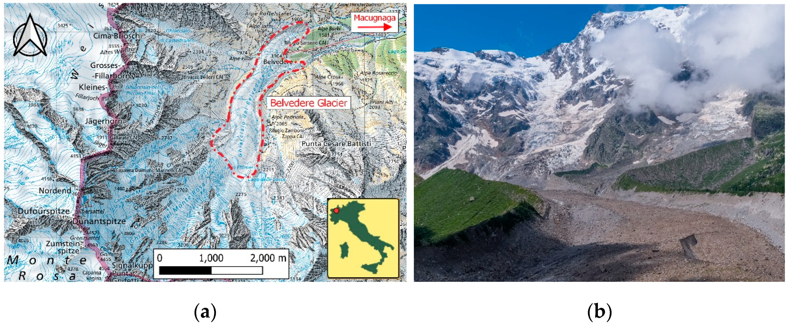
In this framework, the Belvedere Glacier was the object of study because of its peculiar characteristics. It is located at the base of the east side of Monte Rosa (see Figure 1a), in the Anzasca Valley (Piedmont region, Italy). It extends from 1800 to about 2300 m a.s.l., near the municipality of Macugnaga. Belvedere Glacier is a typical dark, debris-covered glacier, almost completely covered by rocks and debris (see Figure 1b), and it is fed by ice and snow avalanches falling from the steep Monte Rosa glacier, which is more than 4500 m high a.s.l. Particularly relevant is the fact that, until the first years of the 21st century, the Belvedere Glacier was one of the few alpine glaciers not retreating. By contrast, between 2000 and 2001, the Belvedere Glacier experienced an extraordinary surge phenomenon: a sudden increase of ice mass at the base of the Monte Rosa glacier propagated down to the valley in the form of a kinematic wave [30,31,32,33].
This work analyzed the evolution of the Belvedere Glacier by means of SfM techniques applied to digitalized historical aerial images combined with more recent digital surveys, either from aerial platforms or UAVs. This allowed the monitoring of an Alpine glacier with high resolution and geometrical accuracy over a long span of time, which is crucial for the considered application. In particular, the period 1977–2019 was considered with five different surveys. The surveys were carried out in different epochs, roughly well distributed in time, so as to capture the morphology of the glacier and quantify volume variations that occurred.
2. Photogrammetric Dataset Description
For the study, data acquired from five photogrammetric surveys performed over a time span ranging between 1977 and 2019 were considered. The earlier datasets (named hereafter historical surveys) dated back to September 1977, August 1991 and September 2001. The images were acquired for regional mapping purposes by the Italian company CGR SpA (Compagnia Generale Ripreseaeree) with analogic photogrammetric cameras mounted aboard planes. The images were catalogued, and their metadata were organized in the SITAD (Sistema Informativo Territoriale Ambientale Diffuso) database [34], now integrated with the GeoPortale Piemonte [35]. Upon request, CGR SpA digitalized the images related to the Belvedere Glacier and made them available to the authors. The analogic films were digitalized by means of a photogrammetric scanner with a resolution of 21 µm/px. The 2009 dataset was also acquired by CGR SpA for mapping purposes (and made available to the authors), but at that time a digital photogrammetric camera was employed. The most recent dataset, from 2019, was directly acquired by the authors by using a fixed-wing UAV with a small and lightweight action camera mounted on board.
A summary of the characteristics of the cameras and flights for each of the five datasets are summarized in Table 1 for immediate comparisons, and more details on these datasets are provided in the following subsections.
2.1. Analog Aerial Datasets of 1977, 1991 and 2001
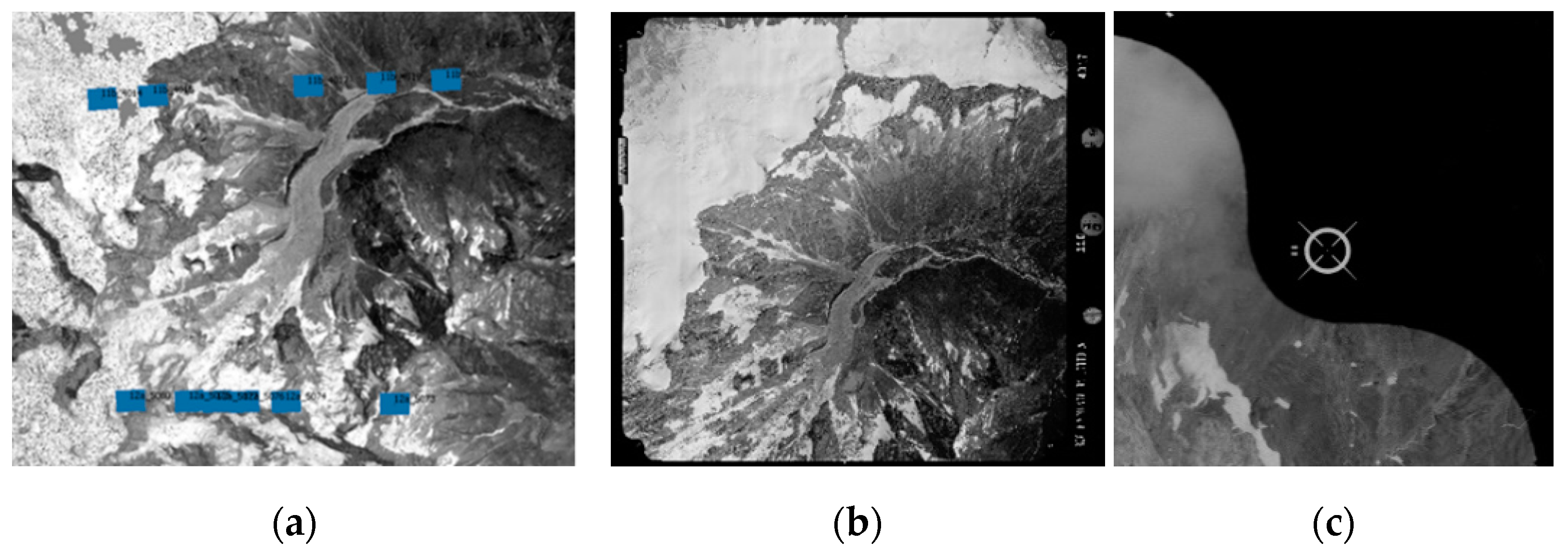
The earliest dataset considered in the study was acquired by CGR SpA on 16/Sep/1977 with an analog photogrammetric camera Wild RC10, equipped with a 15 UAG I lens, with a focal length of 153.26 mm. The flight consisted of three stripes performed at an average altitude of 5600 m a.s.l., with approximately 60% along-flight overlap and transversal overlap varying from 30% to 60% because the stripes were not parallel. A total of 11 RGB images were acquired (see Figure 2). Considering an average altitude of the glacier of 2000 m a.s.l., the scale of the images was about 1:23,000, leading to an average ground sample distance (GSD) of 0.5 m. The camera reference system was materialized on the film with four fiducial marks placed at the four corners of the image. As is visible in Figure 2c, some of the fiducial marks were faded due to the aging of the films, but they were still identifiable in the digitalized images.
The 1991 survey was carried out on two different days: 3/Aug/1991 and 7/Aug/1991. Eleven grayscale images were taken with an analog photogrammetric camera, a Wild RC20 equipped with a 15/4 UAGA F lens (focal length of 153.26 mm). The flight consisted of only two stripes (Figure 3), conducted at 8200 m a.s.l. and 8500 m a.s.l., leading to an average GSD for the images of about 0.9 m. The along-flight overlap was approximately between 70% and 80%, while the transversal overlap was about 50%. As in the images of 1977, four fiducial marks allowed for the definition of the camera reference system (Figure 3c).
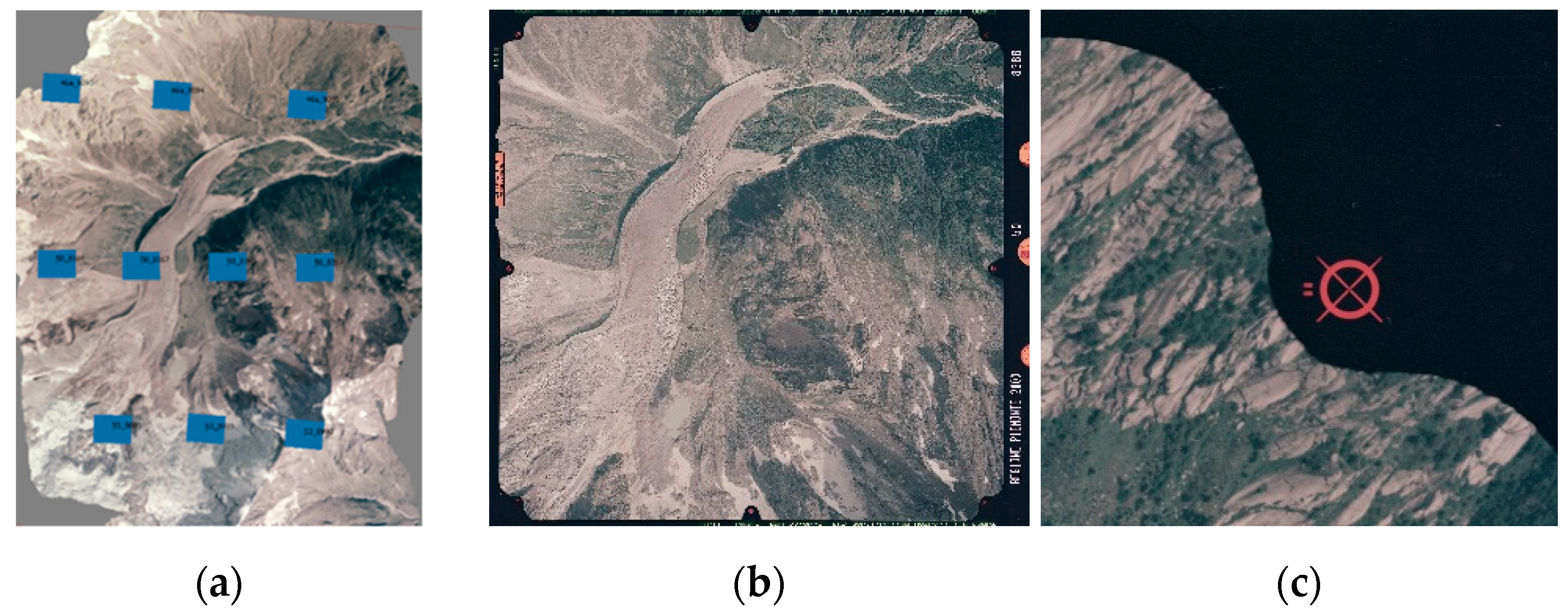
The most recent among the three historical datasets dated back to 2001. Images were acquired with a film camera Wild RC30 equipped with a 15/4 UAG-S lens (focal length of 153.928 mm). The flight consisted of three stripes acquired between 6/Sep/2001 and 11/Sep/2001, producing a total of 10 RGB images with overlaps of ~70% along flight and ~50% in the transversal direction (Figure 4). The two external stripes were conducted at an altitude of about 6100 m a.s.l., while the central one was conducted at a lower altitude of about 4800 m a.s.l, for an average of 5800 m a.s.l. The mean scale of the images was 1:23,000, producing a GSD of 0.5 m, comparable to that of the 1977 flight. The camera reference frame was materialized by 8 fiducial marks, well identifiable on the digitalized images (Figure 4c).
Analog images taken during the aerial surveys of 1977, 1991 and 2001 were digitalized by means of a photogrammetric scanner (PhotoScan2000, developed by Z/I Imaging and Carl Zeiss) capable of scanning analog film rolls. The Photoscan2000 scanner was equipped with a Kodak KLI trilinear CCD sensor with an optical scanning resolution of 7 µm. Pixels could be digitally aggregated to obtain resolutions of 14, 21, 28, 56, 112 or 224 µm. The scanner was designed to ensure a geometrical accuracy for the digitalized images of 2 µm. The images from the historical surveys were digitalized by CGR SpA with a resolution of 21 µm/px, producing eight-bit TIF images with dimensions of 12,098 × 11,144 px. In order to assess the quality of the digitalized images, the actual pixel size was empirically estimated as the ratio of the average distance, in millimeters, of the four fiducial marks at corners and the correspondent average distance in terms of pixels on the digitalized images. The estimated pixel size was 21 µm × 21 µm for each dataset, with computed standard deviations of about three orders of magnitude less, in agreement with the technical specifications of the scanner.
2.2. Digital Aerial and UAV Datasets of 2009 and 2019
During October 2009, a flight over Belvedere Glacier was carried out by CGR SpA for mapping purposes. This time, a digital photogrammetric camera was employed. A Z/I-Imaging DMC camera equipped with a 120 mm focal length lens and a CCD sensor with pixel size of 12 µm × 12 µm, acquiring RGB digital images at a resolution of 7680 × 13,824 pixels, was mounted on an airplane. Eleven images with along-flight and transversal overlaps of 70% and 50%, respectively, were gathered along two stripes with altitude between 5600 and 6000 m a.s.l (Figure 5). The average image scale was 1:32,000, and the GSD was 0.4 m.
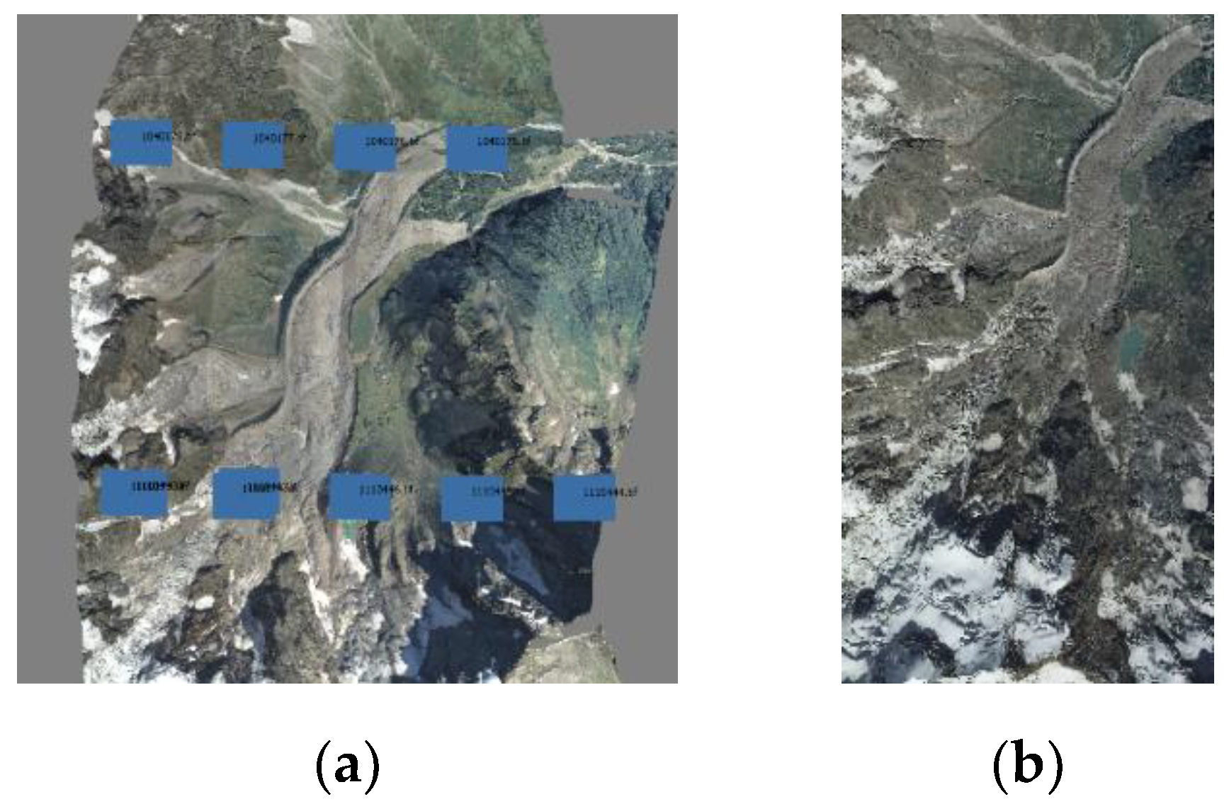
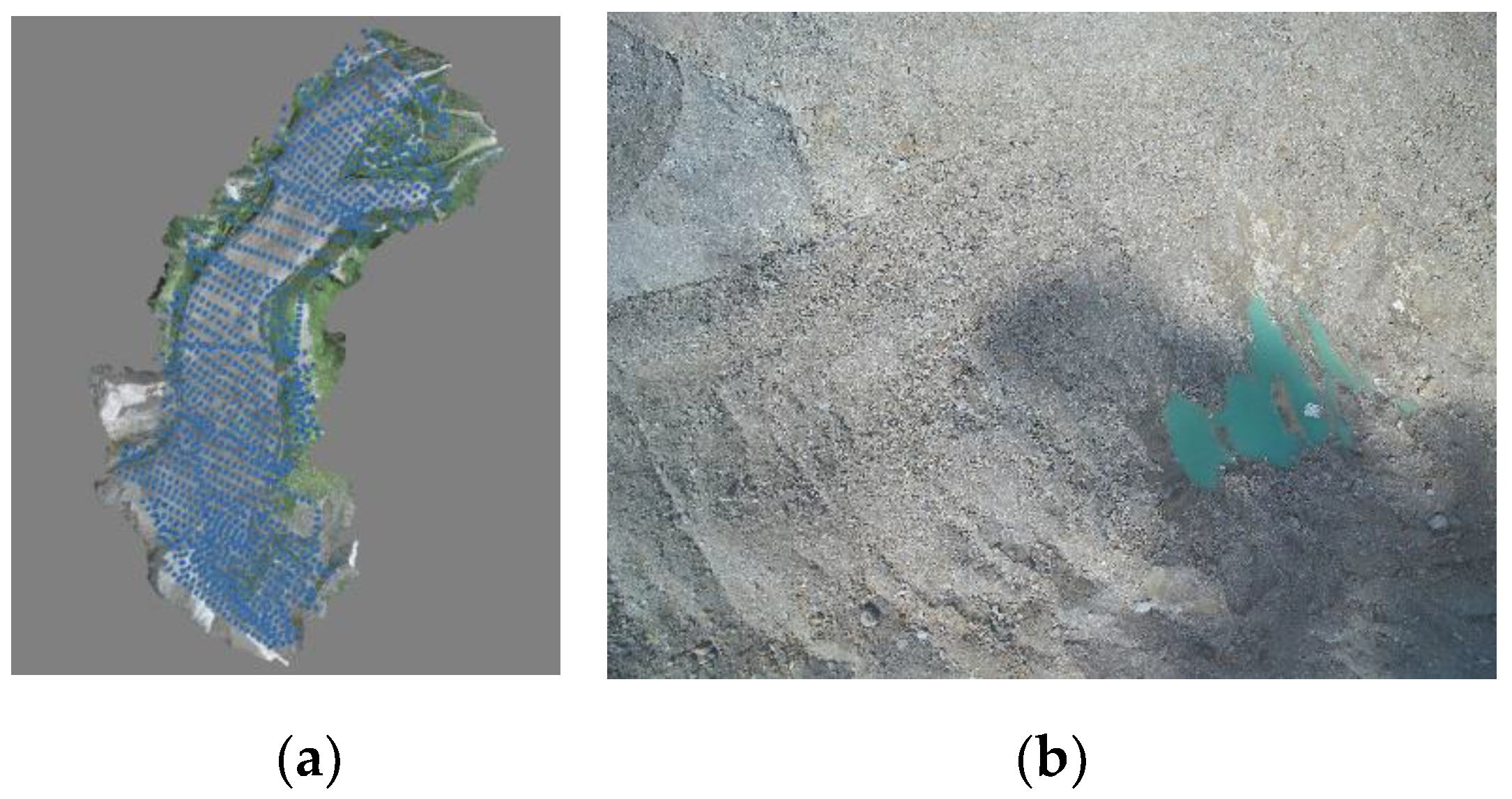
Images from the latest dataset were gathered by the authors during fieldwork on the Belvedere Glacier carried out between 29/Jul/2019 and 2/Aug/2019. A fixed-wing UAV Parrot Disco was adapted in such a way as to carry a low-cost and lightweight action camera, a HawkEye Firefly 8S. The action camera was equipped with a 12 Mpx 1/2.3″ CMOS sensor and had a pixel size of 1.34 µm × 1.34 µm and a focal length of 3.8 mm (90° field of view). The flights were conducted at an average height of 120 m a.g.l. (above ground level), in agreement with Italian UAV regulations, and images were taken with longitudinal and transversal overlap of 80% and 60%, respectively (except for a small portion in the middle of the glacier with a slightly smaller transversal overlap of ~50%; see Figure 6a). The average image scale was therefore approximately 1:32,000, and the GSD was 5 cm, one order of magnitude smaller compared to those of the aerial datasets. Because of UAV technical limitations, the survey area was restricted to the glacier body only and five flights with the fixed-wing UAV were performed (Figure 6).
The characteristics of the cameras and flights for each of the five datasets are summarized in Table 1 for immediate comparison.
2.3. The GNSS Survey for Block Georeferencing
To constrain the UAV photogrammetric block from 2019, 36 squared targets, consisting of 50 cm × 50 cm polypropylene sheets with high color contrast, were deployed over the survey area, anchored to large rocks on both the glacier and the moraines. Among the 36 targets, 26 were used as ground control points (GCPs) and 10 as control points (CPs). The targets were measured on the field with a dual frequency (L1/L2) geodetic quality GNSS receiver Leica GS14. Because GSM internet connection was available in the lower part of the glacier, the targets were measured in nRTK with respect to the HxGN SmartNet network of permanent stations. All the points measured in nRTK were occupied for ~10 s at 1 Hz of acquisition rate. In the upper part of the glacier, where nRTK was not possible, the targets were measured by static positioning. For each of those points, carrier-phase raw observations were logged for a timespan of ~10 min (1 Hz sampling rate). These were postprocessed with respect to a local master station (Leica GPS1200) placed over a target located next to the Zamboni–Zappa hut (2070 m a.s.l.). Coordinates of the master station were repeatedly measured in different years with both static and nRTK measurements, and accuracy on the order of 0.5 cm in planimetry and 2 cm in height was obtained. GNSS observations were postprocessed with the software Leica Infinity (version 3.2.0) in the official Italian reference system ETRF2000 at epoch 2008.0. The resulting accuracies of the coordinates of the GCPs were 1.5 cm in planimetry and 3 cm in height, in terms of average RMSE.
3. Image Orientation and Point Cloud Generation
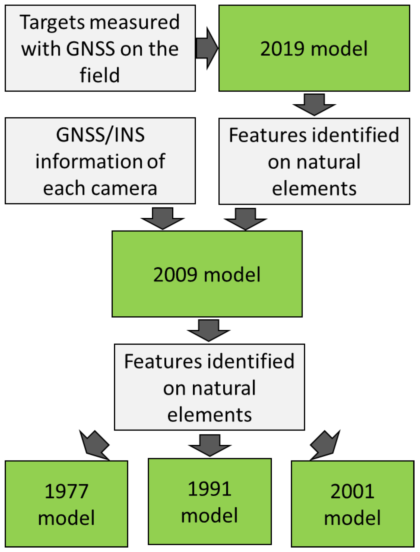
For image orientation and model reconstruction of all the datasets, the photogrammetric software Agisoft Metashape (version 1.7.2) was employed. A sketch of the followed workflow is provided in Figure 7.
Concerning the most recent UAV survey, that from 2019, the 1486 images were oriented by traditional aerial triangulation on the basis of 26 targets spread over the survey (Figure 8) area used as GCPs (see Section 2.2) in the bundle block adjustment (BBA). The GCPs were manually collimated on the images. A collimation accuracy of 1 px was assumed as the a priori standard deviation of the observations within the BBA. Tie Points (TPs) were automatically detected and matched by Metashape on full resolution images. Camera internal orientation (IO) parameters of the Hawkeye Firefly 8S action camera was estimated during the BBA by self-calibration. To this end, approximated values of IO were precalibrated by using a traditional checkerboard. However, these initial values were adjusted for each flight because of the internal instability of the camera and thanks to the high density of the GCPs available.
Regarding the 2009 digital dataset, the DMC system described in Section 2.2 included high-precision GNSS/INS instrumentations able to provide the camera with external orientation (EO) [36]. The coordinates of the camera projection centers were provided with an accuracy of 30 cm, while the camera attitude angles had accuracies of 8 mgon for roll and pitch angles and 10 mgon for yaw [37]. In order to improve the quality of the photogrammetric block within a small area such as that of Belvedere Glacier, 11 features clearly identifiable on the images (e.g., sharp rocks) were used as GCPs. Their coordinates were retrieved from the 2019 model, which had a significantly higher spatial resolution (see Table 1). The EO of the images was estimated through assisted aerial triangulation (AAT) [16]. The BBA was solved by combining GNSS/INS information with TPs automatically detected by the software and 11 GCPs manually collimated on the images. The quality of the photogrammetric model was assessed by means of six check points (CP) not used to solve the BBA.
After the digitalization, the three historical datasets, those from 1977, 1991 and 2001 were oriented by aerial triangulation on the basis of the already-oriented 2009 survey. The coordinates of nine groups of GCPs (marked with numbers 1 to 9 in Figure 8) and eight groups of CPs (marked with letters A to H), well distributed over the whole area, were retrieved from the aerial images acquired with the DMC digital photogrammetry system.
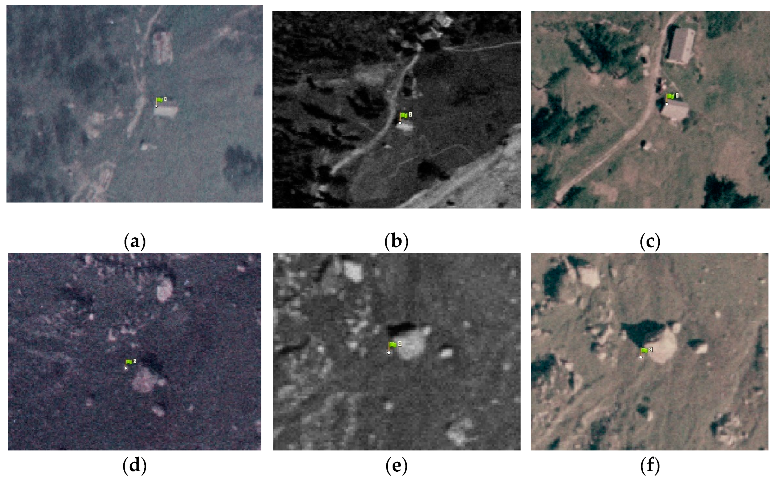
Points such as buildings edges, corners, sharp rocks along the glacier moraines and particular morphological patterns that remained reasonably unchanged over time were selected in such a way as to be clearly identified in most of the four datasets (1977, 1991, 2001 and 2009), as shown in Figure 9.
Note that it was not always possible to identify the same point in all four of the datasets because of the different image scales, different image quality (e.g., RGB versus grayscale images) or changes in the morphology over 30 years. To overcome this problem, if one point was not visible in one dataset, another one was searched nearby. To clarify, if one point (e.g., Point 2) was not found in images from 1991 (e.g., because of the larger image scale), then another feature, named Point 2b, was searched for close to the original location of Point 2 in the 2009 images and used as GCP for the 1991 dataset. However, in the statistics, Points 2 and 2b were considered as one single point because of their spatial proximity.
The GCPs used to solve the BBA of the three historical datasets were properly weighted with their variance. An accuracy of 0.75 px was assumed as the collimation accuracy for a human operator dealing with high-quality digital images such as those from 2009. This assumption was confirmed by the image reprojection error of the manually collimated points, which was always smaller than one pixel. Therefore, an a priori accuracy of 0.3 m was given to the GCPs in the three datasets from 1977, 1991 and 2001.
Concerning the camera IO, the three analog cameras were calibrated in laboratory by the producer, and calibration certificates were available. Therefore, the calibrated value of focal length and the coordinates of the principal point were provided as initial values in the BBA. These were then adjusted based on the GCPs by using a self-calibration procedure [38]. Additionally, two radial (k1 and k2) and tangential (p1 and p2) distortion parameters were estimated in order to correct the lens distortions of the photogrammetric cameras and the distortion introduced by external factors, e.g., the deterioration of the films over the years.
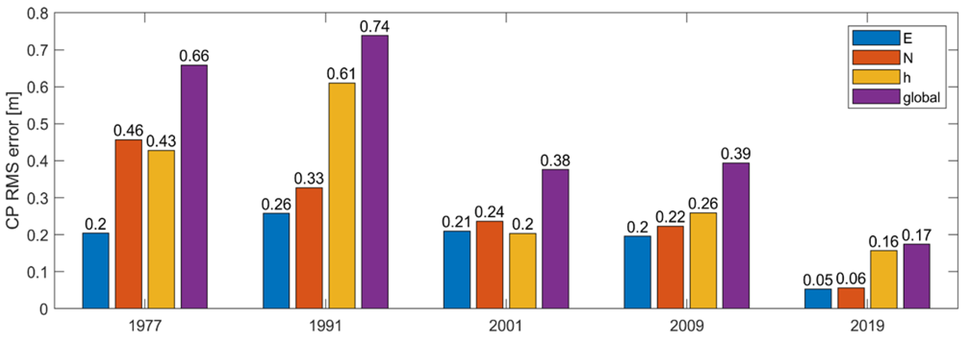
On the basis of the considered CPs, different model accuracies were obtained. The accuracy of the three historical models was assessed by using eight CPs, distributed mainly along the glacier moraines (see Figure 8). Six CPs were used for the 2009 dataset. As reported in Figure 10, the 1977 and 1991 models obtained global RMSEs of about 0.66 m and 0.74 m, respectively, while the 2001 and 2009 models obtained similar RMSEs of about 0.38 m. In all cases, these values were comparable to the average GSD of the aerial images. Regarding the 2019 survey, the model accuracy was assessed by 10 CPs, resulting in a RMSE error of 0.17 m, comparable to three times the GSD. This was due to the low quality of the camera employed. Nevertheless, as the GSD was on the order of magnitude of the centimeter, the model accuracy was still higher than that of the older flights.
Once camera EO was performed by aerial triangulation, georeferenced dense point clouds (PCs) were computed (a downscale factor of 2 was set to make the PCs more manageable) and used as starting point for glacier analyses. The number of points in each PC and the density of each dense cloud are summarized in Table 2.
While the PC size was strictly related to the survey coverage, the PC average density was directly related to the GSD of the original photogrammetric survey, indicating the capability of resolving smaller details.
4. Digital Surface Model Preliminary Processing
The obtained point clouds referring to the different surveys required some additional preprocessing aimed at making them consistent for further analyses. Two main aspects had to be considered: the different average point cloud density and the area coverage. For this purpose, suitable resampling, masking and interpolation of the computed point clouds had to be applied with the aim of obtaining digital surface models (DSMs) in the form of matrices suitable for comparison with each other and quantitative analyses.
4.1. Surface Spatial Resolution Optimization
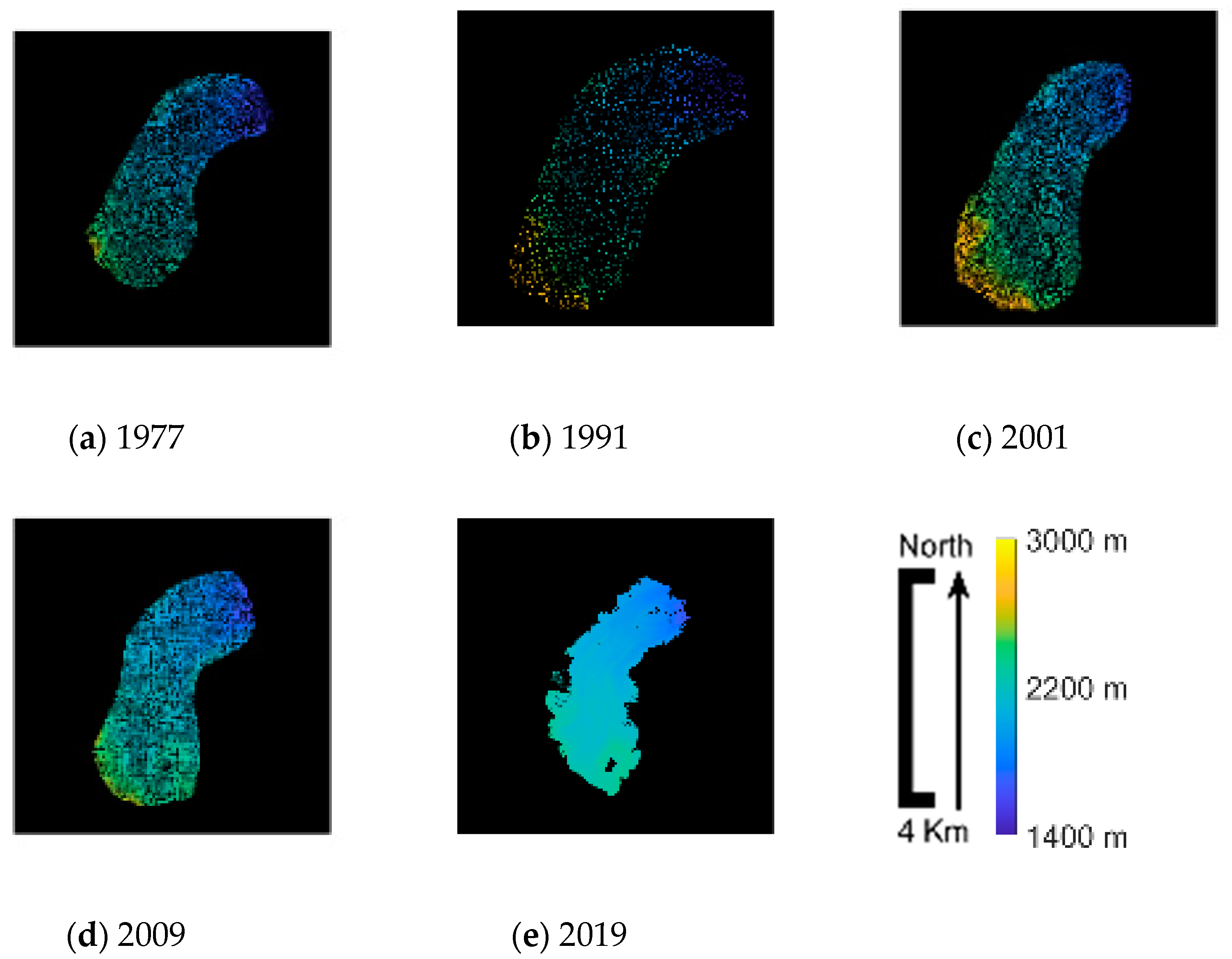
Each of the five point clouds was initially manipulated with CloudCompare (v2.12 alpha). In particular, they were rasterized by exporting them as East–North gridded data with 0.5 m grid spacing and grid knot values corresponding to the average height of the points for which the vertical projection was located in the same grid cell. Empty cells were initially filled with null values. As result, matrices such as those presented in Figure 11 were obtained, suitable for manipulation in the MATLAB (R2020a Update4) environment. The surveyed area can be easily recognized despite the voids (null values) because of the different densities of the input point clouds.
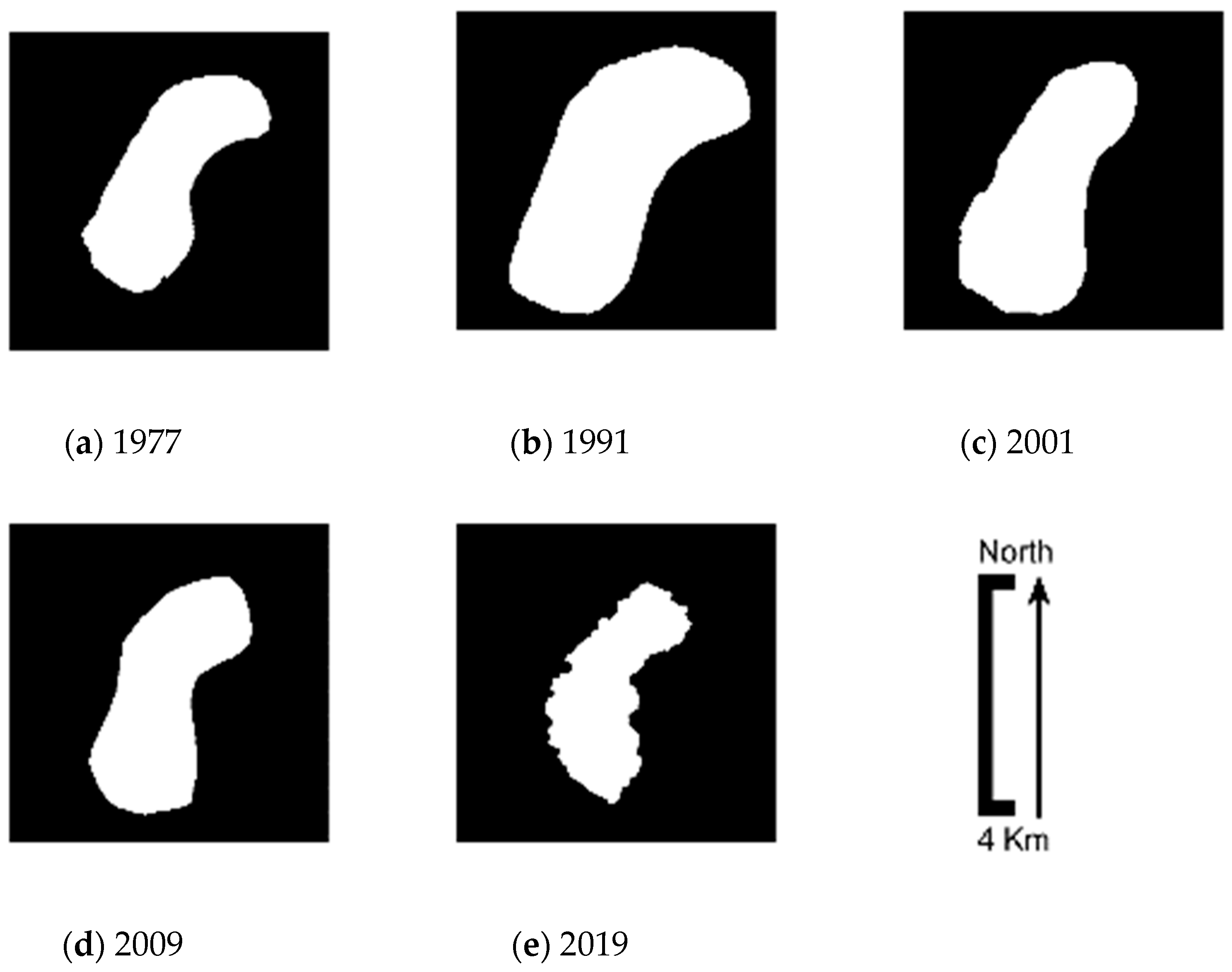
A mask defining each survey area was determined by means of a binary matrix (initially obtained assigning the value 1 to surveyed cells and 0 to missing data) that was refined in a two-step procedure. First, the binary matrix was blurred by iterative convolutions with a kernel representing a circular box (10 m of radius) and assigning unitary value to resulting cells with values greater than 0. As a result, at each iteration, voids were gradually filled, and the inner area was enlarged. Iterations stopped when no voids were present in the inner area. The second step consisted of recovering the initial size of the inner area. By applying the converse procedure (i.e., blurring with the same kernel and assigning 0 to resulting cells with values smaller than 1) for the same number of iterations, a binary mask defining the original surveyed area was obtained. Figure 12 shows the result of this procedure applied to the matrices previously presented in Figure 11.
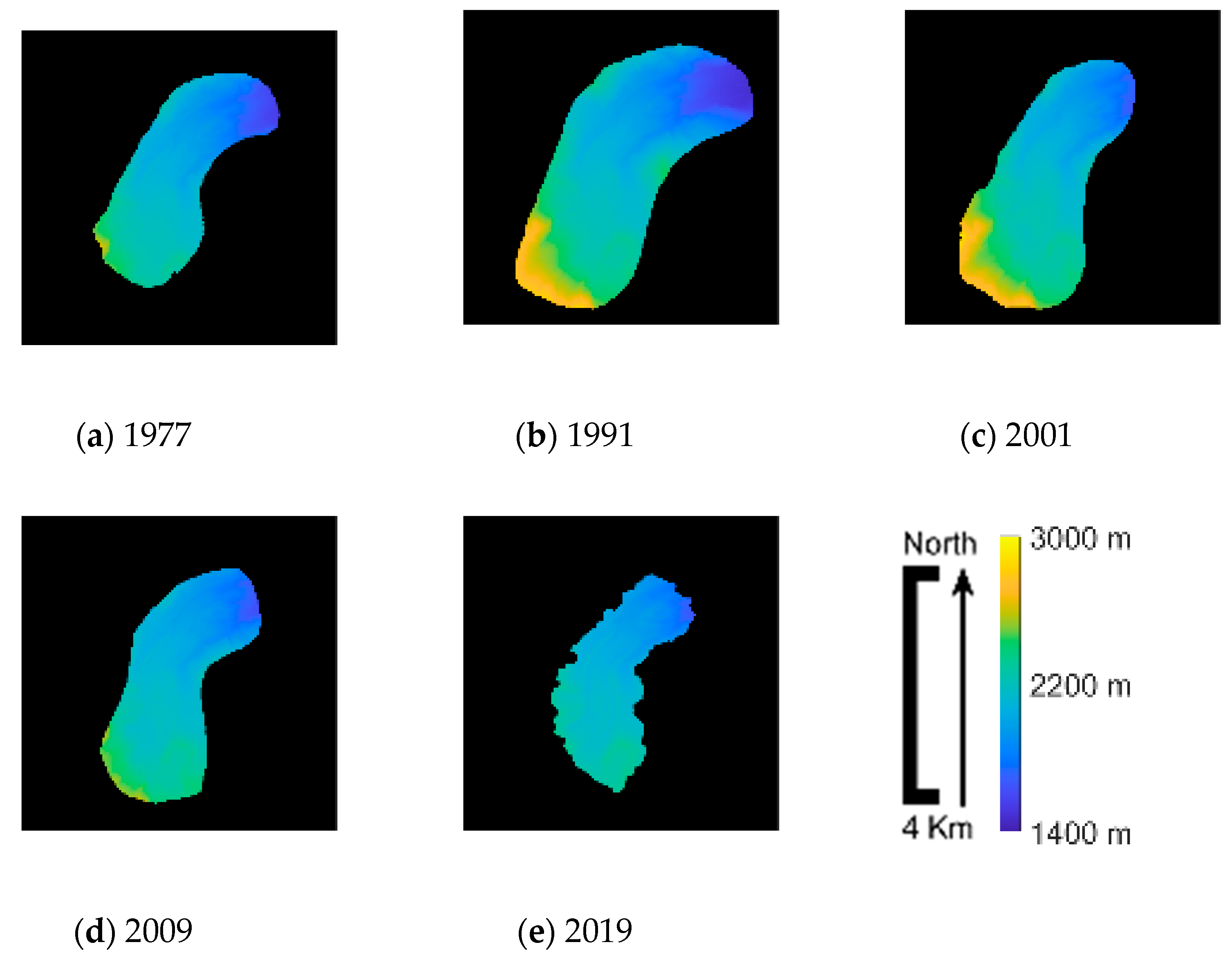
Subsequently, empty cells of initial gridded point clouds were filled via triangulation-based bidimensional linear interpolation. By applying the previously computed survey area masks to the interpolated matrices, artefacts due to extrapolation along the borders of the inner area were filtered out. As result, gridded point clouds at a consistent resolution of 0.5 m were obtained for all five surveys, as presented in Figure 13.
One the basis of this preliminary processing, reliable estimates of surveyed surface coverage and average density of the original point clouds were quantified. In fact, by multiplying the number of nonzero values of the binary masks and the cell size (0.25 m2) of the matrices representing the gridded point clouds, data surface coverage was obtained. Furthermore, the ratio between the number of nonempty cells in the original and interpolated matrices provided an indication of the average data density of the point clouds in the considered surveyed areas. Table 3 summarizes this information for the five analyzed surveys.
The numbers in Table 3 allow evaluating the impact of the chosen grid spacing when gridding the point clouds. With 0.5 m grid spacing, the 2019 survey (that is, the most detailed one, with the lowest flight altitude and average GSD, as reported in Table 1) required few empty cells to be interpolated, about 6%, thus closely fully exploiting its high spatial resolution. A finer grid would require increasing the number of interpolated cells (and thus increasing the required memory allocation for matrix manipulation without adding information), while a coarser one would require downsampling the surveyed detailed DSM, potentially losing finer details. With the chosen grid spacing, the minimum amount of interpolation was needed, while the full potential of more recent and detailed surveys was preserved. Furthermore, the surface coverage of the different surveys was quite different, introducing the second aspect to be addressed to complete the required preprocessing of the point clouds.
4.2. Glacier Mask Determination
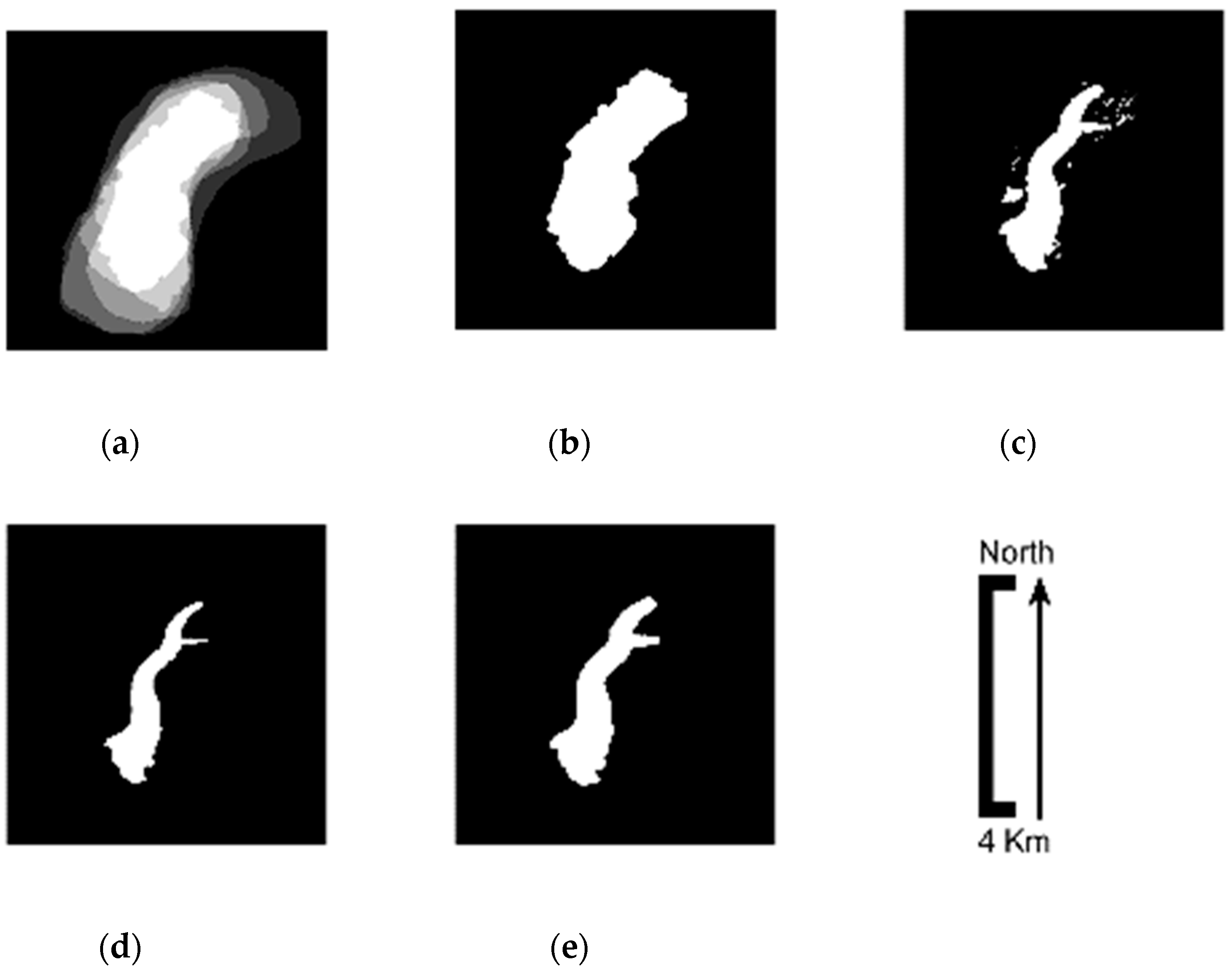
Comparative analyses between the computed DSMs, now at consistent spatial resolution (0.5 m), required the definition of a mask identifying common cells between the interpolated matrices as well as cells referring to the glacier only, excluding surroundings not subject to investigation. For this purpose, the five binary masks were superimposed to each other (Figure 14a) and only fully overlapped cells were considered (Figure 14b). For the identification of the glacier boundaries, a data-driven approach was pursued. Low or even null altitude variability over time was expected in the surrounding areas, while cells referring to the glacier body were expected to show detectable changes in altitude. Figure 12c shows the binary mask representing those cells for which the height difference between consecutive survey epochs was greater than 10 m. The shape of the glacier body is clearly recognizable. This mask was then refined by applying the same iterative procedure previously presented for survey edge identification, which first removed isolated areas and cleaned glacier borders (Figure 14d) and then applied a buffer around it so as to also comprise lateral moraines expected to remain almost unchanged over time (Figure 14e). The obtained final binary mask (now covering about a surface of 1.78 km2) referring to the glacier only was then applied to the interpolated matrices, now made fully consistent for the detection of glacier changes.
5. Glacier Analyses
The final masked DSMs allowed spatial analyses of the glacier surface by comparing the measured altitude variations. Information on dynamics, evolution and volume ablation/accumulation could quantified during the considered timespan, from 1977 to 2019. First, the DSMs were analyzed in absolute terms, i.e., in terms of their altitude variability range and the spatial distribution of areas classified on the basis of their measured altitude. Table 4 shows the surveyed minimum and maximum altitudes. The minimum values were more or less similar, within 5 m of variability, the while maximum values ranged between about 2339 and 2385 m. The stability of the minimum values can be justified by the area masking. Minimum altitudes likely occurred in the vicinity of the glacier terminus, and the mask buffering could have comprised points surveyed at the terminus foot, where transported rock deposits and debris were present in different positions along the valley. On the other hand, the variability of the maximum values can be justified by reversing the analyses. Higher altitudes likely occurred closer to mountainous peaks along the surveyed glacier accumulation area, located in the SW region of the mask, where mass balance can benefit from events such as avalanches or particular meteorological conditions immediately before the epoch of the surveys.
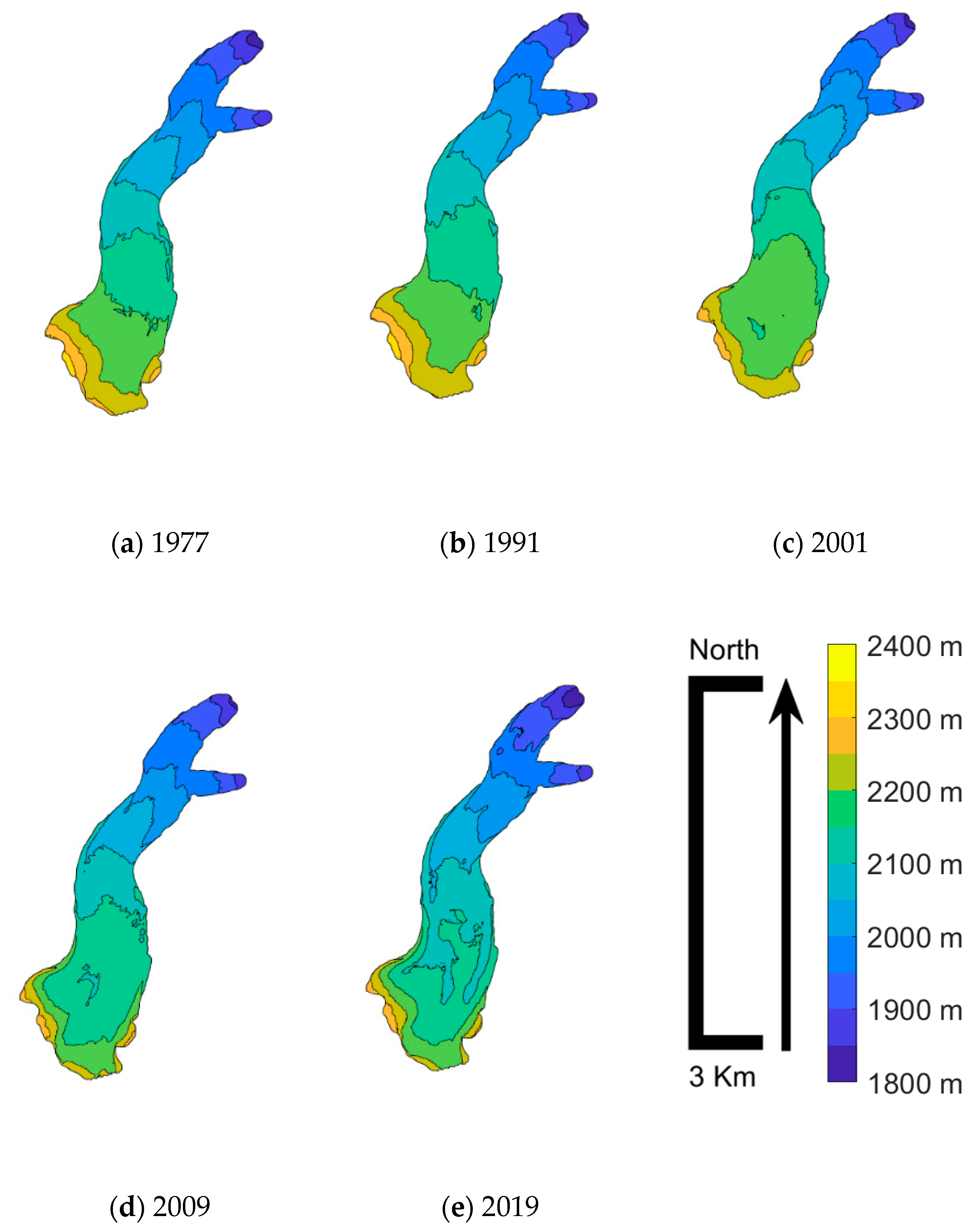
Other information was extrapolated by analyzing the spatial distribution of the measured altitudes. In this sense, the evolution in time of the glacier contours provided immediate feedback on the glacier’s surface dynamics. Figure 15 presents glacier contour altitudes between 1800 and 2400 m, so as to comprise the maximum altitude range measured by the five surveys with a contour interval of 50m. With respect to the 1977 DSM (Figure 15a), 1991 DSM cells classified in the range 2200–2400 m remained almost unchanged while the following contour lines gradually moved toward a valley, clearly indicating a mass accumulation (Figure 15b). The following 2001 survey showed a continuation in these areas of the trend of increasing altitude toward the glacier terminus, but an altitude decrease was observed in the SW cells of the accumulation area (note the extension of the altitude class 2200–2250 m in Figure 15c), and cells of the highest altitude class were practically absent (see Table 4). The 2009 DSM showed totally different behavior (Figure 15d). Lower contour lines retreated toward peaks, approximately in the same location as in 1977, while the 2150–2200 m range greatly retreated and covered a large part of the glacier toward the accumulation area. The most recent 2019 DSM (Figure 15e) again showed a general retreat trend of lower contour lines, with no sharp transition in the range of 2100–2200 m (probably due to high surface ablation phenomena) and no great variation in the remaining areas in the range of 2200–2350 m.
In order to quantify the different effects of accumulation and ablation processes on Belvedere Glacier during time, relative comparisons were conducted. As previously clarified, because the different DSMs were georeferenced and made consistent in terms of spatial resolution, volume variations could be computed by considering DSM altitude variations and cell size. Cumulate volume variations were obtained, taking the 1977 DSM as reference, while average annual volume losses/gains were obtained in the considered periods. Table 5 reports these relative comparisons.
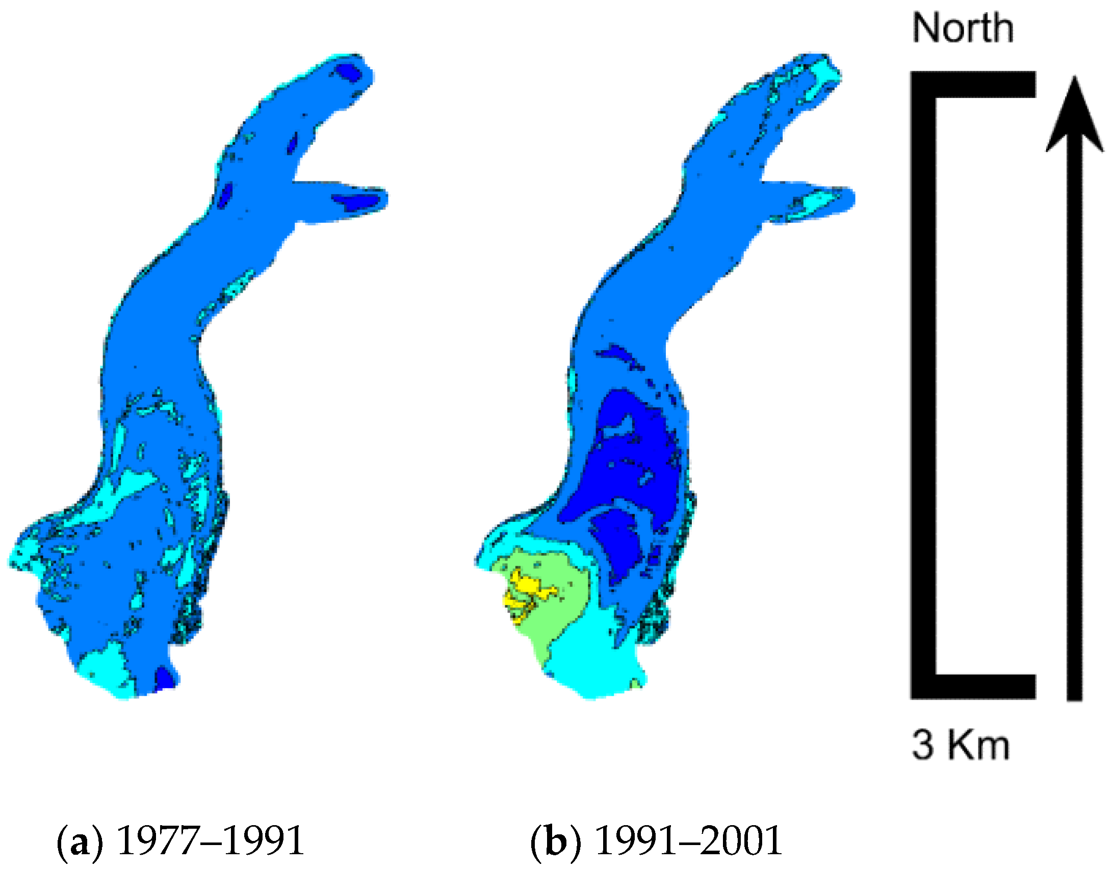
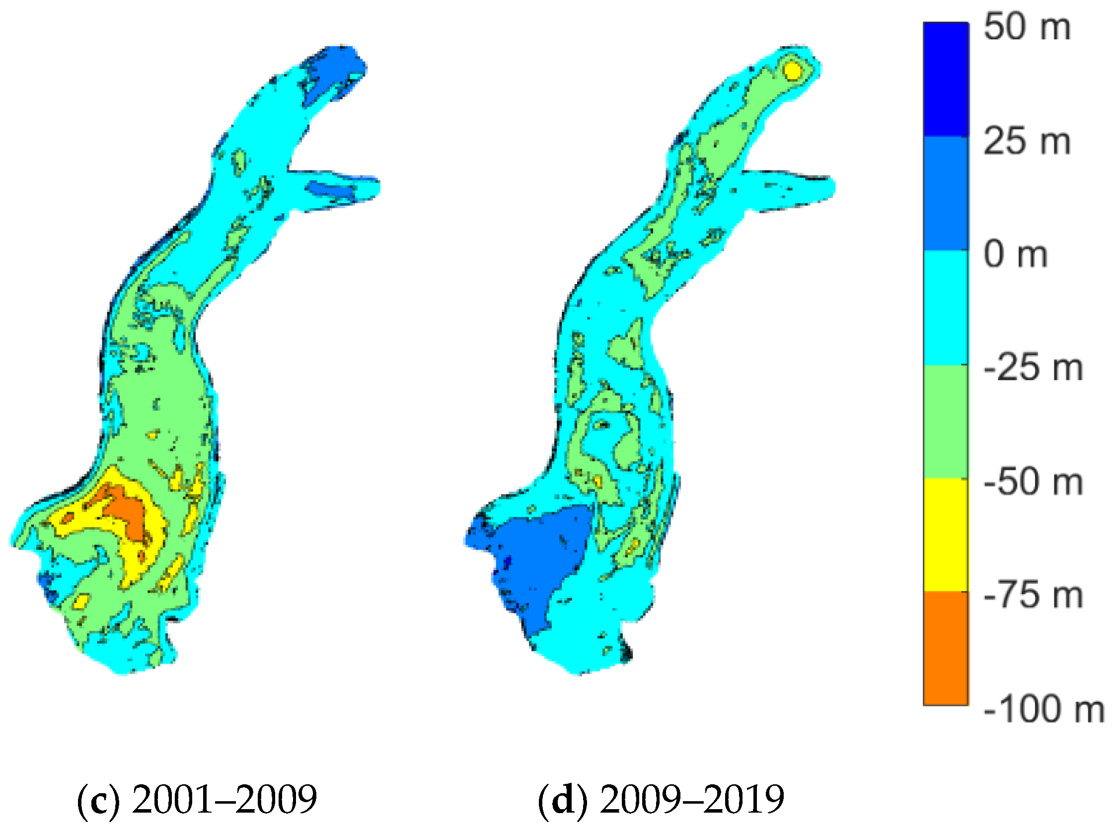
The numbers in Table 5 confirm what was found by analyzing the glacier contours variations, but from a different perspective. In the period 1977–2001, the glacier’s volume increased by about +20.66 million m3, and its rate of volume gain increased by about 50% in the period 1991–2001 (from +0.72 to +1.06 million m3/year). The period 2001–2019 revealed an important reduction of glacier volume. In the period 2001–2009, the average yearly volume decrease was −5.97 million m3/year, bringing the volume down to −27.12 million m3 with respect to the initial volume recorded in 1977 despite the volume accumulation in the previous period. In the following period, between 2009 and 2019, the trend remained negative but was less severe (−2.72 million m3/year), resulting in a total loss of −54.28 million m3 in the considered 42 years, from 1977 to 2019. The reported volume gains or losses refer to the whole glacier surface, but it could be interesting to investigate local variations. Figure 16 classifies glacier areas in terms of altitude variation, with contour intervals of 25 m. In the first considered period, from 1977 to 1991, the volume increase was quite distributed. Glacier terminus advancement was clearly visible, and volume decrease was measured in small portions at higher altitudes. The following period, 1991–2001, saw an important volume accumulation in the central part of the glacier, which was partially counterbalanced at higher altitudes. The following periods showed general volume loss, which was particularly important between 2001 and 2009 in the higher portion and was distributed until the terminus (see the northern one) in the period 2009–2019.
6. Conclusions
This work analyzed the evolution of the Belvedere Glacier by means of SfM techniques applied to digitalized historical aerial images combined with more recent digital surveys, either from aerial platforms or UAVs. This allowed the monitoring of the Belvedere Glacier with high resolution and geometrical accuracy over a long span of time, which is crucial for this application. Digital surface models of the area surrounding the glacier were produced on the basis of five different surveys conducted at the epochs 1977, 1991, 2001, 2009 and 2019 with different ground resolutions and accuracies, which for the most recent survey even reached the decimeter level. First, DSMs were made comparable by producing georeferenced raster images at equal spatial resolution (with common cell size of 0.5 m). Then, proper masks focusing on the glacier surface were determined by following a data-driven approach and exploiting common image processing techniques. This preprocessing led to the determination of glacier altitude and volume variations during the considered time span, sampled about every 10 years. Volume gains/losses were clearly identified and, more importantly, quantified. In the period 1977–2019, a loss of about 54 million m3 was computed, but the trend of these losses was far from linear. In the first half of the considered period, the glacier increased its volume and extent, accelerating this phenomenon in the second period. In the second half, a sudden glacier retreat began, particularly severe in the first decade of the current century, that almost totally compensated the volume increase of the previous 20 years. In the last period, the retreat continued, bringing us the current state of the glacier with thickness reduced by tenths of meters, particularly at higher altitudes. Without the use of historical aerial acquisitions, such long-term analyses would have suffered from a lack of data referring to less recent epochs that was suitable to be processed and made consistent with most recent technologies. This proved how the availability of such data is a remarkable heritage for glaciological studies.
Author Contributions
The authors declare equal contributions to this research. All authors have read and agreed to the published version of the manuscript.
Funding
This research received no external funding.
Data Availability Statement
Restrictions apply to the availability of these data. Data was obtained from CGR SpA and are available from the authors with the permission of CGR SpA.
Acknowledgments
The authors wish to thank CGR SpA for the digitalization of the historical datasets and for making available their proprietary datasets.
Conflicts of Interest
The authors declare no conflict of interest.
References
- Rogora, M.; Frate, L.; Carranza, M.L.; Freppaz, M.; Stanisci, A.; Bertani, I.; Bottarin, R.; Brambilla, A.; Canullo, R.; Carbognani, M.; et al. Assessment of Climate Change Effects on Mountain Ecosystems through a Cross-Site Analysis in the Alps and Apennines. Sci. Total Environ. 2018, 624, 1429–1442. [Google Scholar] [CrossRef] [Green Version]
- Sommer, C.; Malz, P.; Seehaus, T.C.; Lippl, S.; Zemp, M.; Braun, M.H. Rapid Glacier Retreat and Downwasting throughout the European Alps in the Early 21st Century. Nat. Commun. 2020, 11, 1–10. [Google Scholar] [CrossRef]
- Zekollari, H.; Huss, M.; Farinotti, D. Modelling the Future Evolution of Glaciers in the European Alps under the EURO-CORDEX RCM Ensemble. Cryosphere 2019, 13, 1125–1146. [Google Scholar] [CrossRef] [Green Version]
- Auer, I.; Böhm, R.; Jurkovic, A.; Lipa, W.; Orlik, A.; Potzmann, R.; Schöner, W.; Ungersböck, M.; Matulla, C.; Briffa, K.; et al. HISTALP-Historical Instrumental Climatological Surface Time Series of the Greater Alpine Region. Int. J. Climatol. 2007, 27, 17–46. [Google Scholar] [CrossRef]
- Marty, C.; Meister, R. Long-Term Snow and Weather Observations at Weissfluhjoch and Its Relation to Other High-Altitude Observatories in the Alps. Theor. Appl. Climatol. 2012, 110, 573–583. [Google Scholar] [CrossRef] [Green Version]
- Eder, K.; Würländer, R.; Rentsch, H. Eder, Konrad, Roland Würländer, and Hermann Rentsch. Digital photogrammetry for the new glacier inventory of Austria. Int. Arch. Photogramm. Remote Sens. 2000, 33, 254–261. [Google Scholar]
- Knoll, C.; Kerschner, H. A Glacier Inventory for South Tyrol, Italy, Based on Airborne Laser-Scanner Data. Ann. Glaciol. 2009, 50, 46–52. [Google Scholar] [CrossRef] [Green Version]
- Smiraglia, C.; Azzoni, R.S.; D’Agata, C.; Maragno, D.; Fugazza, D.; Diolaiuti, G.A. The Evolution of the Italian Glaciers from the Previous Data Base to the New Italian Inventory. Preliminary Considerations and Results. Geogr. Fis. Din. Quat. 2015, 38, 79–87. [Google Scholar]
- Legat, K.; Moe, K.; Poli, D.; Bollmann, E. Exploring the Potential of Aerial Photogrammetry for 3D Modelling of High-Alpine Environments. Int. Arch. Photogramm. Remote Sens. Spat. Inf. Sci. 2016, 9, 97–103. [Google Scholar] [CrossRef] [Green Version]
- Kaufmann, V. The Evolution of Rock Glacier Monitoring Using Terres-Trial Photogrammetry: The Example of Äußeres Hoch-Ebenkar Rock Glacier (Austria). Aust. J. Earth Sci. 2012, 105, 63–77. [Google Scholar]
- Kääb, A. Monitoring High-Mountain Terrain Deformation from Repeated Air-and Spaceborne Optical Data: Examples Using Digital Aerial Imagery and ASTER Data. ISPRS J. Photogramm. Remote Sens. 2002, 57, 39–52. [Google Scholar] [CrossRef]
- Kaufmann, V.; Ladstädter, R. Quantitative Analysis of Rock Glacier Creep by Means of Digital Photogrammetry Using Multi-Temporal Aerial Photographs: Two Case Studies in the Austrian Alps. In Proceedings of the 8th International Conference on Permafrost, Zurich, Switzerland, 21–25 July 2003; pp. 21–25. [Google Scholar]
- Keutterling, A.; Thomas, A. Monitoring Glacier Elevation and Volume Changes with Digital Photogrammetry and GIS at Gepatschferner Glacier, Austria. Int. J. Remote Sens. 2006, 27, 4371–4380. [Google Scholar] [CrossRef]
- Fieber, K.D.; Mills, J.P.; Miller, P.E.; Clarke, L.; Ireland, L.; Fox, A.J. Rigorous 3D Change Determination in Antarctic Peninsula Glaciers from Stereo WorldView-2 and Archival Aerial Imagery. Remote Sens. Environ. 2018, 205, 18–31. [Google Scholar] [CrossRef]
- Giulio Tonolo, F.; Cina, A.; Manzino, A.; Fronteddu, M. 3D Glacier Mapping by Means of Satellite Stereo Images: The Belvedere Glacier case study in the Italian Alps. Int. Arch. Photogramm. Remote Sens. Spat. Inf. Sci. 2020, 43, 1073–1079. [Google Scholar] [CrossRef]
- Ioli, F.; Pinto, L.; Ferrario, F. Low-Cost DGPS Assisted Aerial Triangulation for Sub-Decimetric Accuracy with NON-RTK UAVs. Int. Arch. Photogramm. Remote Sens. Spat. Inf. Sci. 2021, 43, 25–32. [Google Scholar] [CrossRef]
- Bhardwaj, A.; Sam, L.; Martín-Torres, F.J.; Kumar, R. UAVs as Remote Sensing Platform in Glaciology: Present Applications and Future Prospects. Remote Sens. Environ. 2016, 175, 196–204. [Google Scholar] [CrossRef]
- Immerzeel, W.W.; Kraaijenbrink, P.D.A.; Shea, J.M.; Shrestha, A.B.; Pellicciotti, F.; Bierkens, M.F.P.; De Jong, S.M. High-Resolution Monitoring of Himalayan Glacier Dynamics Using Unmanned Aerial Vehicles. Remote Sens. Environ. 2014, 150, 93–103. [Google Scholar] [CrossRef]
- De Michele, C.; Avanzi, F.; Passoni, D.; Barzaghi, R.; Pinto, L.; Dosso, P.; Ghezzi, A.; Gianatti, R.; Della Vedova, G. Using a Fixed-Wing UAS to Map Snow Depth Distribution: An Evaluation at Peak Accumulation. Cryosphere 2016, 10, 511–522. [Google Scholar] [CrossRef] [Green Version]
- Gindraux, S.; Boesch, R.; Farinotti, D. Accuracy Assessment of Digital Surface Models from Unmanned Aerial Vehicles’ Imagery on Glaciers. Remote Sens. 2017, 9, 186. [Google Scholar] [CrossRef] [Green Version]
- Avanzi, F.; Bianchi, A.; Cina, A.; De Michele, C.; Maschio, P.; Pagliari, D.; Passoni, D.; Pinto, L.; Piras, M.; Rossi, L. Centimetric Accuracy in Snow Depth Using Unmanned Aerial System Photogrammetry and a Multistation. Remote Sens. 2018, 10, 765. [Google Scholar] [CrossRef] [Green Version]
- Rossini, M.; Di Mauro, B.; Garzonio, R.; Baccolo, G.; Cavallini, G.; Mattavelli, M.; De Amicis, M.; Colombo, R. Rapid Melting Dynamics of an Alpine Glacier with Repeated UAV Photogrammetry. Geomorphology 2018, 304, 159–172. [Google Scholar] [CrossRef]
- Fugazza, D.; Scaioni, M.; Corti, M.; D’Agata, C.; Azzoni, R.S.; Cernuschi, M.; Smiraglia, C.; Diolaiuti, G.A. Combination of UAV and Terrestrial Photogrammetry to Assess Rapid Glacier Evolution and Map Glacier Hazards. Nat. Hazards Earth Syst. Sci. 2018, 18, 1055–1071. [Google Scholar] [CrossRef] [Green Version]
- Jouvet, G.; Weidmann, Y.; Kneib, M.; Detert, M.; Seguinot, J.; Sakakibara, D.; Sugiyama, S. Short-Lived Ice Speed-up and Plume Water Flow Captured by a VTOL UAV Give Insights into Subglacial Hydrological System of Bowdoin Glacier. Remote Sens. Environ. 2018, 217, 389–399. [Google Scholar] [CrossRef]
- Chudley, T.R.; Christoffersen, P.; Doyle, S.H.; Abellan, A.; Snooke, N. High-Accuracy UAV Photogrammetry of Ice Sheet Dynamics with No Ground Control. Cryosphere 2019, 13, 955–968. [Google Scholar] [CrossRef] [Green Version]
- Geissler, J.; Mayer, C.; Jubanski, J.; Münzer, U.; Siegert, F. The potentials of high-resolution photogrammetry for analyzing glacier retreat in the Ötztal Alps, Austria. Cryosphere 2020, 1–22. [Google Scholar] [CrossRef]
- Westoby, M.J.; Brasington, J.; Glasser, N.F.; Hambrey, M.J.; Reynolds, J.M. “Structure-from-Motion” Photogrammetry: A Low-Cost, Effective Tool for Geoscience Applications. Geomorphology 2012, 179, 300–314. [Google Scholar] [CrossRef] [Green Version]
- Ryan, J.C.; Hubbard, A.L.; Box, J.E.; Todd, J.; Christoffersen, P.; Carr, J.R.; Holt, T.O.; Snooke, N. UAV Photogrammetry and Structure from Motion to Assess Calving Dynamics at Store Glacier, a Large Outlet Draining the Greenland Ice Sheet. Cryosphere 2015, 9, 1–11. [Google Scholar] [CrossRef] [Green Version]
- Poli, D.; Casarotto, C.; Strudl, M.; Bollmann, E.; Moe, K.; Legat, K. Use of Historical Aerial Images for 3D Modelling of Glaciers in the Province of Trento. ISPRS Int. Arch. Photogramm. Remote Sens. Spat. Inf. Sci. 2020, XLIII-B2, 1151–1158. [Google Scholar] [CrossRef]
- Mazza, A. Evolution and Dynamics of Ghiacciaio Nord Delle Locce (Valle Anzasca, Western Alps) from 1854 to the Present. Geogr. Fis. Din. Quat. 1998, 21, 233–243. [Google Scholar]
- Haeberli, W.; Kääb, A.; Paul, F.; Chiarle, M.; Mortara, G.; Mazza, A.; Deline, P.; Richardson, S. A Surge-Type Movement at Ghiacciaio Del Belvedere and a Developing Slope Instability in the East Face of Monte Rosa, Macugnaga, Italian Alps. Nor. Geogr. Tidsskr. 2002, 56, 104–111. [Google Scholar] [CrossRef]
- Kääb, A.; Huggel, C.; Barbero, S.; Chiarle, M.; Cordola, M.; Epifani, F.; Haeberli, W. Glacier Hazards At Belvedere Glacier and the Monte Rosa East Face, Italian Alps: Processes and Mitigation. Inter. Natl. Symp. 2004, 67–78. [Google Scholar]
- Mondino, E.B.; Chiabrandoa, R. Multi-temporal block adjustment for aerial image time series: The Belvedere glacier case study. ISPRS-Int. Arch. Photogramm. Remote Sens. Spat. Inf. Sci. 2008, 37, 89–94. [Google Scholar]
- Cipriano, P. ITAD: Building Spatial Data Infrastructure in Italy. In GIS for Sustainable Development, 1st ed.; CRC Press: Boca Raton, FL, USA, 2005; pp. 489–499. [Google Scholar]
- Geoportale Piemonte. Available online: http://www.geoportale.piemonte.it/geocatalogorp/index.jsp (accessed on 3 April 2021).
- Hinz, A.; Dörstel, C.; Heier, H. The Digital Sensor Technology of Z/I-Imaging. In Photogrammetric Week; Cite Seerx: University Park, PA, USA, 2001; pp. 93–103. [Google Scholar]
- Forlani, G.; Pinto, L. Integrated INS/DGPS systems: Calibration and combined block adjustment. In Proceedings of the OEEPE workshop Integrated Sensor Orientation, Hannover, Germany, 17–18 September 2001; Heipke, C., Jacobsen, K., Wegmann, H., Eds.; Bundesampt fur Kartographie und Geodasie: Frankfurt, Germany, 2001. [Google Scholar]
- Jacobsen, K. Issues and Method for In-Flight and On Orbit Calibration, Workshop on Radiometric and Geometric Calibration. In Proceedings of the International Workshop on Radiometric and Geometric Calibration, Gulfport, MS, USA, 2–5 December 2003. [Google Scholar]
Figure 1.
(a) Location of Belvedere Glacier, base map (source: Swisstopo www.geo.admin.ch, accessed on 10 August 2021); (b) view of Monte Rosa from the Belvedere Glacier surface (photograph by Francesco Ioli).
Figure 1.
(a) Location of Belvedere Glacier, base map (source: Swisstopo www.geo.admin.ch, accessed on 10 August 2021); (b) view of Monte Rosa from the Belvedere Glacier surface (photograph by Francesco Ioli).

Figure 2.
(a) Sketch of the 1977 aerial acquisitions; (b) sample image; (c) fiducial mark example.

Figure 3.
(a) Sketch of the 1991 aerial acquisitions; (b) sample image; (c) fiducial mark example.

Figure 4.
(a) Sketch of the 2001 aerial acquisitions; (b) sample image; (c) fiducial mark example.

Figure 5.
(a) Sketch of the 2009 aerial acquisitions; (b) sample image.

Figure 6.
(a) Sketch of the 2019 UAV acquisitions; (b) sample image.

Figure 7.
Workflow for the reconstruction of models and their spatial alignment in a common reference frame.
Figure 7.
Workflow for the reconstruction of models and their spatial alignment in a common reference frame.

Figure 8.
Sketches of the GCP and CP locations: (a) 1977, 1991 and 2001 surveys; (b) 2009 survey; (c) 2019 survey.
Figure 8.
Sketches of the GCP and CP locations: (a) 1977, 1991 and 2001 surveys; (b) 2009 survey; (c) 2019 survey.

Figure 9.
Examples of points chosen as GCPs or CPs. (a–c), artificial features in 1977, 1991 and 2001 aerial images, respectively; (d–f), natural features in 1977, 1991 and 2001 aerial images, respectively.
Figure 9.
Examples of points chosen as GCPs or CPs. (a–c), artificial features in 1977, 1991 and 2001 aerial images, respectively; (d–f), natural features in 1977, 1991 and 2001 aerial images, respectively.

Figure 10.
Model accuracy comparison in terms of RMS error on CPs.

Figure 11.
Initial rasterized point clouds: (a) 1977; (b) 1991; (c) 2001; (d) 2009; (e) 2019.

Figure 12.
Binary masks defining the survey coverage: (a) 1977; (b) 1991; (c) 2001; (d) 2009; (e) 2019.
Figure 12.
Binary masks defining the survey coverage: (a) 1977; (b) 1991; (c) 2001; (d) 2009; (e) 2019.

Figure 13.
Interpolated gridded point clouds: (a) 1977; (b) 1991; (c) 2001; (d) 2009; (e) 2019.

Figure 14.
Final mask for defining the glacier boundaries: (a) binary mask overlaps; (b) common area; (c) high-variability area; (d) filtered high-variability area; (e) buffered high-variability area, i.e., considered glacier shape.
Figure 14.
Final mask for defining the glacier boundaries: (a) binary mask overlaps; (b) common area; (c) high-variability area; (d) filtered high-variability area; (e) buffered high-variability area, i.e., considered glacier shape.

Figure 15.
Glacier contours at different epochs: (a) 1977; (b) 1991; (c) 2001; (d) 2009; (e) 2019.

Figure 16.
Binned glacier altitude variations in different periods with bin size set to 25 m: (a) 1977–1991; (b) 1991–2001; (c) 2001–2009; (d) 2009–2019.
Figure 16.
Binned glacier altitude variations in different periods with bin size set to 25 m: (a) 1977–1991; (b) 1991–2001; (c) 2001–2009; (d) 2009–2019.


Table 1.
Summary of camera and flight characteristics for the five datasets.
| 1977 | 1991 | 2001 | 2009 | 2019 | |
|---|---|---|---|---|---|
| Camera | Wild RC10 | Wild RC20 | Wild RC30 | Z/I-Imaging DMC | Hawkeye Firefly 8S |
| Support/sensor | 230 × 230 mm film | 230 × 230 mm film | 230 × 230 mm film | CCD sensor | 1/2.3″ CMOS sensor |
| Lens | 15 UAG I | 15/4 UAGA-F | 15/4 UAG-S | 4 × f = 120 mm/f:4.0 | integrated |
| Focal length (mm) | 153.260 | 152.820 | 153.928 | 120.000 | 3.800 |
| Pixel size (µm2) | 21 × 211 | 21 × 21 1 | 21 × 21 1 | 12 × 12 | 1.34 × 1.34 |
| Avg flight h AGL (m) | 3600 | 6400 | 3500 | 3800 | 120 |
| Avg image scale | 1:23,000 | 1:42,000 | 1:23,000 | 1:32,000 | 1:32,000 |
| Avg GSD (m) | 0.50 1 | 0.90 1 | 0.50 1 | 0.40 | 0.05 |
1 For analog images, pixel size and GSD refer to those of the digitalized images.
Table 2.
Point cloud (PC) numbers of points and volumetric densities.
| 1977 | 1991 | 2001 | 2009 | 2019 | |
|---|---|---|---|---|---|
| PC size (pts) | 8,962,182 | 4,296,638 | 12,504,582 | 17,595,703 | 112,293,439 |
| PC average density (pts/m3) | 1.56 | 1.08 | 1.58 | 2.67 | 26.40 |
Table 3.
Surface coverage of the binary masks and percentage of noninterpolated data within the covered area.
Table 3.
Surface coverage of the binary masks and percentage of noninterpolated data within the covered area.
| 1977 | 1991 | 2001 | 2009 | 2019 | |
|---|---|---|---|---|---|
| surface coverage (km2) | 5.53 | 9.41 | 7.17 | 5.98 | 4.33 |
| average data coverage | 37% | 11% | 39% | 60% | 94% |
Table 4.
Minimum and maximum altitudes (a.s.l.) of the glacier at different epochs.
| Epoch | 1977 | 1991 | 2001 | 2009 | 2019 |
|---|---|---|---|---|---|
| min altitude (m) | 1820.72 | 1823.60 | 1824.44 | 1826.23 | 1825.64 |
| max altitude (m) | 2381.11 | 2385.07 | 2350.37 | 2339.43 | 2349.36 |
Table 5.
Glacier volume gain/loss in the four considered periods.
| Period | 1977–1991 | 1991–2001 | 2001–2009 | 2009–20019 |
|---|---|---|---|---|
| ΔVol (millions m3) | +10.06 | +10.61 | −47.78 | −27.16 |
| yearly ΔVol (millions m3/year) | +0.72 | +1.06 | −5.97 | −2.72 |
| cumulated ΔVol (millions m3) | +10.06 | +20.66 | −27.12 | −54.28 |
Publisher’s Note: MDPI stays neutral with regard to jurisdictional claims in published maps and institutional affiliations. |
© 2021 by the authors. Licensee MDPI, Basel, Switzerland. This article is an open access article distributed under the terms and conditions of the Creative Commons Attribution (CC BY) license (https://creativecommons.org/licenses/by/4.0/).
Share and Cite
MDPI and ACS Style
De Gaetani, C.I.; Ioli, F.; Pinto, L. Aerial and UAV Images for Photogrammetric Analysis of Belvedere Glacier Evolution in the Period 1977–2019. Remote Sens. 2021, 13, 3787. https://0-doi-org.brum.beds.ac.uk/10.3390/rs13183787
AMA Style
De Gaetani CI, Ioli F, Pinto L. Aerial and UAV Images for Photogrammetric Analysis of Belvedere Glacier Evolution in the Period 1977–2019. Remote Sensing. 2021; 13(18):3787. https://0-doi-org.brum.beds.ac.uk/10.3390/rs13183787
Chicago/Turabian StyleDe Gaetani, Carlo Iapige, Francesco Ioli, and Livio Pinto. 2021. "Aerial and UAV Images for Photogrammetric Analysis of Belvedere Glacier Evolution in the Period 1977–2019" Remote Sensing 13, no. 18: 3787. https://0-doi-org.brum.beds.ac.uk/10.3390/rs13183787
Note that from the first issue of 2016, this journal uses article numbers instead of page numbers. See further details here.