Optimizing the Sowing Date to Improve Water Management and Wheat Yield in a Large Irrigation Scheme, through a Remote Sensing and an Evolution Strategy-Based Approach

Abstract

This study aims to investigate the effects of an optimized sowing calendar for wheat over a surface irrigation scheme in the semi-arid region of Haouz (Morocco) on irrigation water requirements, crop growth and development and on yield. For that, a scenario-based simulation approach based on the covariance matrix adaptation–evolution strategy (CMA-ES) was proposed to optimize both the spatiotemporal distribution of sowing dates and the irrigation schedules, and then evaluate wheat crop using the 2011–2012 growing season dataset. Six sowing scenarios were simulated and compared to identify the most optimal spatiotemporal sowing calendar. The obtained results showed that with reference to the existing sowing patterns, early sowing of wheat leads to higher yields compared to late sowing (from 7.40 to 5.32 t/ha). Compared with actual conditions in the study area, the spatial heterogeneity is highly reduced, which increased equity between farmers. The results also showed that the proportion of plots irrigated in time can be increased (from 40% to 82%) compared to both the actual irrigation schedules and to previous results of irrigation optimization, which did not take into consideration sowing dates optimization. Furthermore, considerable reduction of more than 40% of applied irrigation water can be achieved by optimizing sowing dates. Thus, the proposed approach in this study is relevant for irrigation managers and farmers since it provides an insight on the consequences of their agricultural practices regarding the wheat sowing calendar and irrigation scheduling and can be implemented to recommend the best practices to adopt.

1. Introduction

1.1. Background and Context

In Morocco, cereals are the main cultivated crop, both in terms of utilized agricultural area (UAA), and in terms of value in agricultural production, domestic food security and livestock survival [1]. This agricultural crop covers approximately 5.3 million ha and accounts for 65% of the total cropped area [1]. The production of wheat (durum wheat and common wheat) practiced by almost all Moroccan farmers concerns 3 million ha [1]. However, production remains highly variable from year to year depending on climatic variability, mainly annual precipitation levels, and does not follow national demand, which increases dependence on imports particularly during dry years [2]. Recent studies expected that global warming will threaten most of the world’s wheat production and may cause major droughts in 60% of wheat-growing areas [3]. For Morocco, drought is increasing in frequency and intensity [4]. For instance, the observed annual average temperatures increased every decade since 1970 and the Intergovernmental Panel on Climate Change (IPCC) projected a continued warming trend with an increase of about 1 to 1.5 degrees Celsius by 2050 [5]. Additionally, a recent World Bank study on climate change in Morocco shows that precipitation will decrease by 10 to 35 percent [2].

Several studies showed that high temperature and water deficit during the key reproductive phases have significant effects on the length of the wheat development periods [6] and decrease of wheat yield and grain quality [7,8,9,10,11,12]. Thus, to mitigate the effect of climate change on wheat productivity, conventional agricultural practices such as sowing date must be adjusted to increase yield [13,14,15,16]. Sowing time impacts the duration and timing of developmental phases by avoiding climatic constraints in wheat sensitive stages [15,17,18,19]. Different approaches have been developed to estimate crop sowing dates by defining a set of rules based on crop and climate characteristics [20,21]. In other common approaches, crop models were used to identify the best agricultural practices in a specific climate [22,23], or to study the effect of shifting the sowing date on crop yield [24,25,26,27,28] or to assess crops performance depending on climatic conditions [25,29,30]. Other studies have investigated the effect of spatiotemporal variability in sowing dates, at the regional level, on yield [31,32,33]. But among these studies, few focused on the optimization of the sowing window in arid and semi-arid regions such as Morocco under present climatic conditions [18].

Conversely, water scarcity is one of the key factors limiting agricultural development and thus food security, especially in arid and semi-arid regions where irrigation consumes more than 85% of the available water resources [34]. This is the case of the Haouz plain (central of Morocco), classified as a semi-arid region [35], where water availability is a major limitation for cereal production [36].

In this study, we focused on surface irrigation systems, which occupy about 80% of irrigated areas worldwide [37] and about 76% in Morocco [1], particularly the large-scale irrigation schemes under rotational water supply. It has been demonstrated that existing rules for water distribution among farmers, often based on a fixed-area proportionate depth of water applied in every irrigation round irrespective of the crops and their growth stages, induce an inadequate water supply and have negative effects on wheat productivity [38,39]. The irrigation scheduling approach adopted by the managers results in either an excess of water or a lack of water leading to a more complex management: (1) at the beginning of the agricultural season, the sowing dates depend on the first rainfall and the number of irrigation rounds and water amounts to be applied, depending mainly on the available water resources (the water stored in the dams), (2) for each irrigation round, the irrigation distribution is mainly based on hydraulic and technical constraints (location of the fields, canals discharge, staff operating the water intakes, etc.…) and the starting date is based on visual observations, and (3) water is applied based on a fixed-area proportionate water rate without considering the crop water demand, the crop type and the level of water stress of each crop, which is the most influential factor on crop growth and yield and the heterogeneity of farmers’ behaviors and objectives.

Consequently, efficient and optimized spatiotemporal allocation of irrigation water in a surface irrigation system to improve crop water use efficiency and to ensure adequate productivity in irrigated agriculture during water deficit years is crucial for the sustainability of agricultural development in the arid and semi-arid regions.

1.2. State of the Art

Optimized allocation of limited available irrigation water resources can be achieved by adopting best agricultural practices related mainly to sowing dates and irrigation schedules, while taking into account both the heterogeneity of environmental and agronomic conditions (water stress levels, type of crop, soil characteristics, rainfall, etc.) and the technical and human constraints (behavior of the actors, the different interactions between them, their decision-making strategies, the constraints of the irrigation network, etc.). This is a complex problem that requires a large amount of precise information. However, with help of optimization approaches using mathematical calculation, objective function and existing constraints, it has been possible to handle the complexities of surface irrigation systems.

Many studies have been conducted to address different irrigation water management issues using initial optimization techniques, such as linear programming (LP), nonlinear programming (NLP), integer programming (IP), dynamic programming (DP), and quadratic programming (QP) [40,41,42,43,44]. To cover the drawbacks of these traditional methods, which are time-consuming, intelligent evolutionary algorithms, such as genetic algorithm (GA), evolutionary strategies (ES) and evolutionary programming (EP), has also been widely used in an array of agricultural problems, and their results shown to be more efficient and more promising for finding global optima [45]. For instance [46], comparing five evolutionary algorithms (real valued genetic algorithm, particle swarm optimization, differential evolution, and two evolution strategy-based algorithms) on the problem of irrigation optimization demonstrated that they are able to optimize irrigation schedules, achieving results that are extremely close to the theoretical optimum. The efficiency and the strength of genetic algorithm approach to provide optimal irrigation scheduling has been also demonstrated in several studies [47,48,49,50,51,52].

Among this evolutionary algorithms, the covariance matrix adaptation–evolution strategy (CMA-ES) algorithm is recognized as one of the most powerful methods in the black box continuous optimization framework [53], and it is particularly suited to problems containing many local minimums [54], as presented by the results of the competition at IEEE-CEC 2005 [55] and BBOB workshops at ACM-conferences GECCO 2010, 2011 and 2013 [53]. Comparative analysis with several algorithms has also shown that the CMA-ES algorithm is one of the most effective meta-heuristics for dealing with difficult optimization problems [53]. Unlike genetic algorithms based on biological analogies, CMA-ES uses a space sampling of the parameters by a population of points drawn according to a Gaussian law. The number of individuals depends on the dimensionality of the problem. The CMA-ES algorithm is generally used to search for the solution of complex problems in order to obtain a reasonable calculation time.

In a previous study [56], we have proposed an approach based on the CMA-ES evolutionary strategy algorithm for optimizing irrigation scheduling. The obtained results demonstrate that it can be considered as an efficient tool for planning irrigation schedules by considering crops water needs and timing. This research was conducted in our study area and proposed an optimization during only one irrigation round in a surface irrigation network, without optimizing the spatiotemporal distribution of sowing dates and irrigation rounds along wheat season.

In this context, the present study aims to propose a decision support approach for rational and efficient management of irrigation in large surface irrigation systems, based on an optimization of the spatiotemporal distribution of sowing dates and irrigation, while evaluating the effects on the irrigation rounds scheduling, the consumed irrigation water and the wheat yield. This approach can contribute to the adaptation of agricultural practices to water scarcity conditions and meet food production needs in response to climate change.

2. Materials and Methods

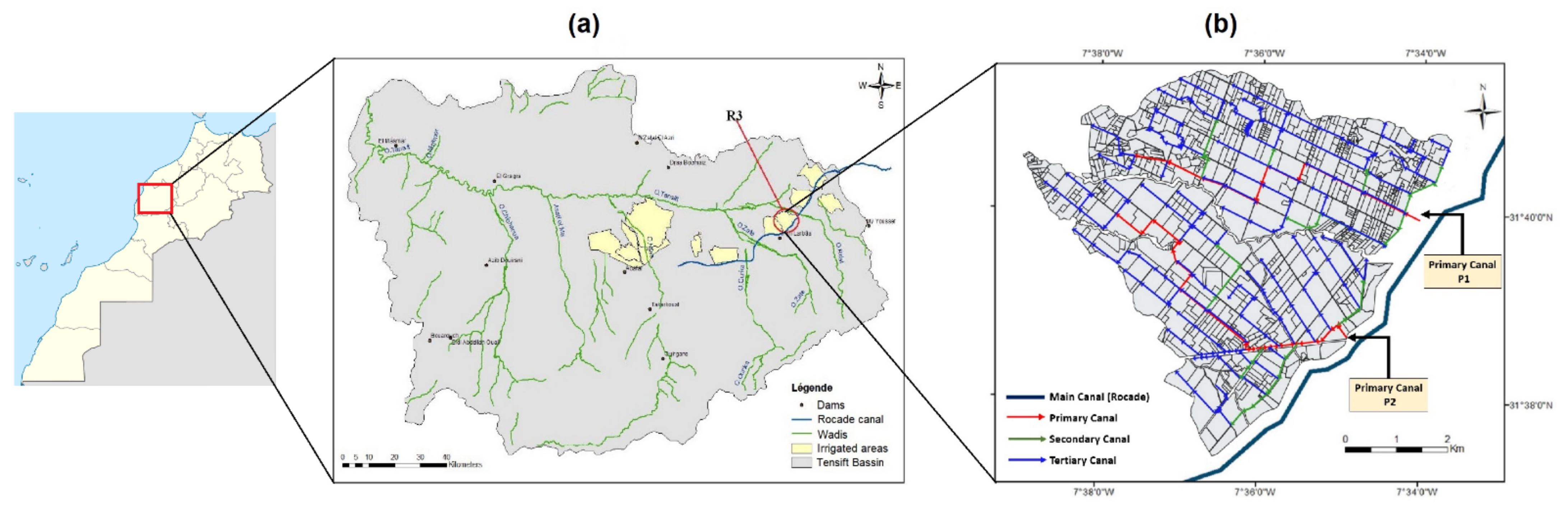
2.1. Study Area

Our study area is located in the Haouz plain (Figure 1a) in the center of the Tensift basin (Central Morocco). It is a vast plain 6000 km² in area (including approximately 3100 km² of irrigated area), characterized by a semi-arid continental climate, with low and irregular rainfall of 250 mm/year on average, a high temperature in summer (38 °C on average, in July) and low temperature in winter (5 °C on average, in February) [57]. Among the irrigated sectors of the Haouz plain, the R3 district (Figure 1b) was chosen as the main area to validate our research results. It is located about 40 km east of Marrakech city and covers an area of 2800 ha composed of around 745 individual fields, used mainly for cereal crops (45% in 2011–2012 and the remainder surface was occupied by annual crops, trees and fallow). R3 is flat and considered by many previous studies as a suitable area for satellite applications (e.g., [34,58,59,60]). At field level, water is applied by flooding method. A fixed water rate is received by each plot, at each irrigation round, without taking into account the type of crops, water requirement, and the cultivated area.

Water is provided to the R3 irrigated area from the “Hassan 1st dam” located in the neighboring catchment of “Oum Er-rbia” via the “Rocade” canal, and through a classical gravity network made of lined canals (Figure 1b). The latter is composed of two primary canals: P1 on the right bank of the sector and P2 on the left bank, and a network of secondary and tertiary open canals convey water to the cropped fields. The entire area is divided into irrigation blocks composed of 6 plots of 4–5 ha each, generally supplied by a tertiary canal feeding 1 to 10 blocks.

Irrigation and land use in this study area is managed jointly by the Regional Office of Agricultural Development of Haouz (ORMVAH) and the water users associations (WUA). Depending on the water allocated to irrigation, managers and WUAs decide the number of irrigation rounds and water rates to apply at each one. Then, the irrigation schedule is implemented throughout the season in collaboration between the ORMVAH and the farmers (i.e., the starting date and duration of each irrigation round), which is usually based on simple observations of weather conditions and/or on a visual assessment of the plants and soil moisture status.

This approach generates a high spatiotemporal heterogeneity of the applied irrigation volumes at the plot scale, whose complexity is usually not considered in the irrigation scheduling process. Thus, an optimized irrigation management for an efficient and productive water use in such complex system should be adopted.

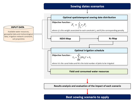
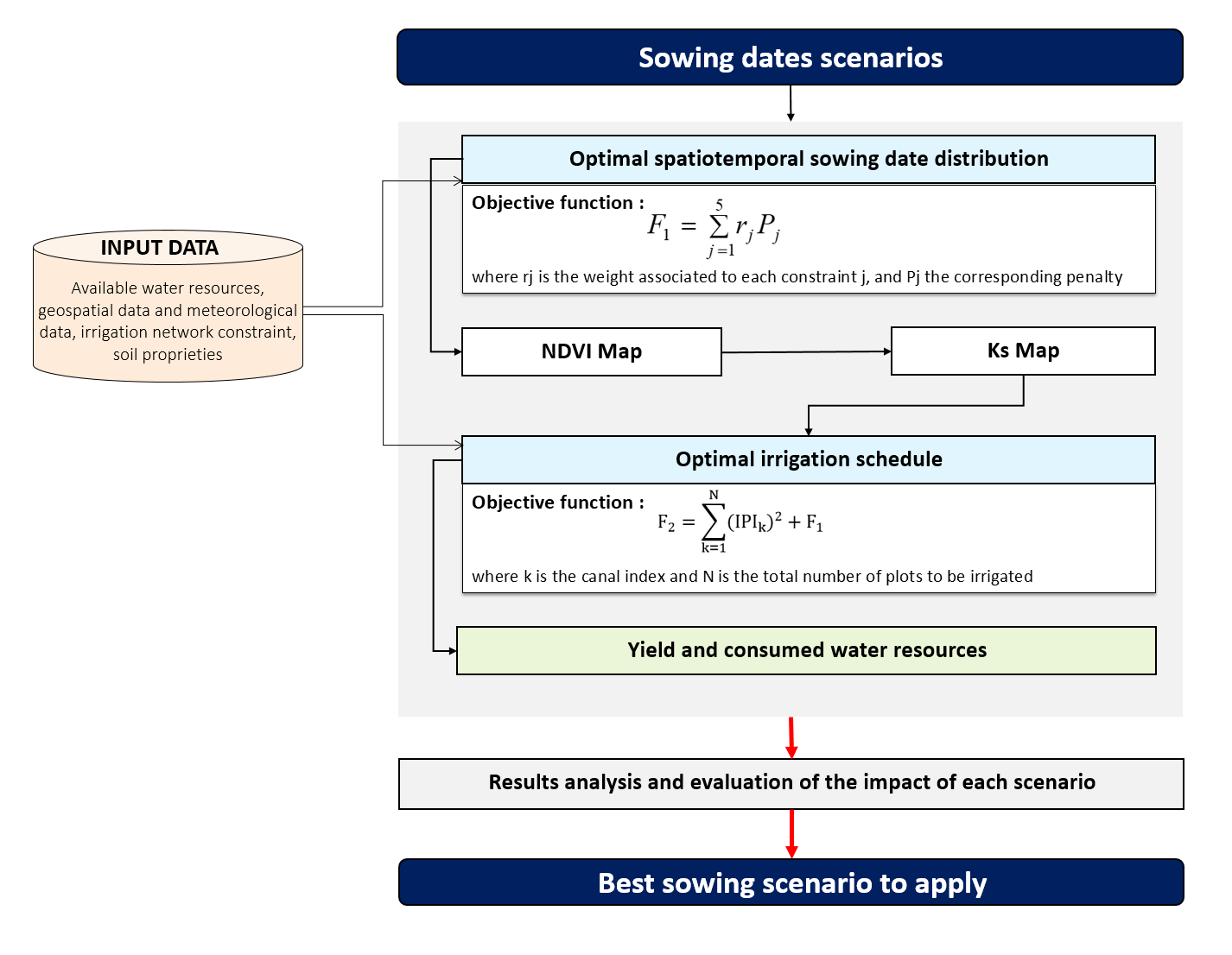
2.2. The Proposed Approach

To help farmers and irrigation scheme managers make good decisions about the winter wheat planting calendar and irrigation schedules that allow optimized water consumption and crop productivity, we propose an innovative approach (Figure 2), which takes place in three phases of the agricultural season:

• At the beginning of the agricultural season, the spatiotemporal distribution of the sowing dates over the irrigation scheme is optimized, considering the irrigation network constraints and the adopted sowing scenario. The number of plots to be sown in a same day is defined based mainly on the capacity of the irrigation network, i.e., the maximum volume of water that can be delivered to the plots irrigated by the same canal, according to its maximum discharge and location (tertiary, secondary or primary). Thus, the total area that will be sown in a given day is determined such that it can be completely irrigated in one single day during an irrigation round;
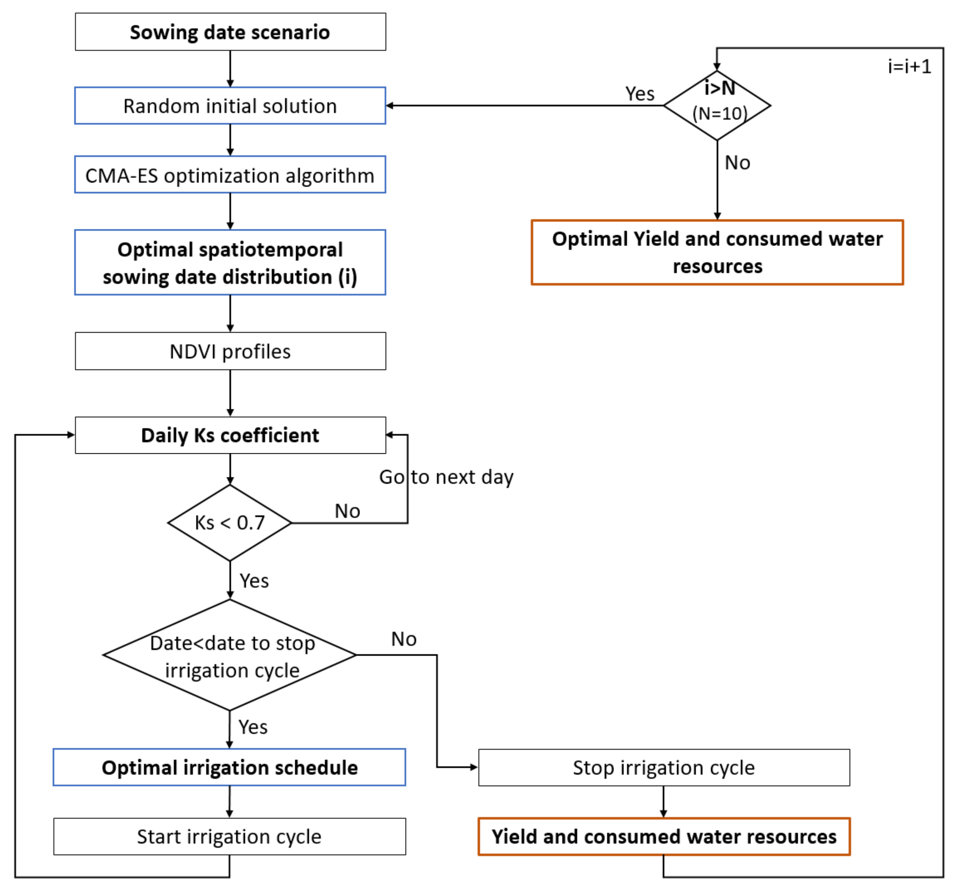
• During the agricultural season, before starting each irrigation round, we elaborate an optimal irrigation planning (irrigation date and irrigation water requirement for each plot) over the irrigation scheme according to the sowing calendar scenario and the crop water stress levels in each field. The starting date of each irrigation round is calculated based on the water stress coefficient (Ks), which is used to measure the soil water deficit levels for the crop, as defined in the FAO56 model [61], based on the Normalized Difference Vegetation Index (NDVI), which is a common and widely used remote sensing index to assess the green biomass and the state and health of crops by measuring the difference between near-infrared and red light. Thus, the Ks is equal to 1 at the day of sowing (because the farmers sow after a heavy rainfall event or a pre-irrigation at the beginning of the season). Then, Ks is calculated using the daily soil water balance at the root zone (see Section 2.3). An irrigation round is decided when the Ks reaches a value less than 0.7 at most for 5% of the total cultivated area. This threshold of Ks has been identified as the value above which the water stress does not affect significantly wheat yield [36,62,63]. Then, for each irrigation round, the spatiotemporal irrigation planning is optimized based on the Irrigation Priority Index (IPI) [56] (see Section 2.4 and Section 2.6). When a plot is irrigated, the Ks coefficient becomes equal to 1 and the process continues to define the starting of the next irrigation round. Additionally, no more irrigation is decided for wheat crop at the end of the season when the canopy cover reaches the half of the maximum canopy cover during the senescence stage (see Section 2.2);
• At the end of the agricultural season, an evaluation of the irrigation water consumed and the final yield expected is conducted in order to decide on the most optimal spatiotemporal sowing date calendar to be adopted, i.e., the best recommendations concerning the cultivation schedule which will allow to increase incomes and reduce the use of water resources during the agricultural season.

The initial distribution of sowing dates is simulated randomly (taking into consideration the window of sowing scenario) to avoid local solutions and to ensure that the best results are independent from these initial values. We reiterate the algorithm 10 times. The solution corresponding to the higher value of the total yield and the lower value of the consumed water resources is considered as the optimal solution.

We applied this approach for wheat plots during 2011–2012 agricultural season over the left side of R3 irrigation scheme irrigated by the primary canal R3P2 (composed of one primary canal, two secondary canals and 30 tertiary canals). The simulations concerned 116 plots, which constitute 45% of the global area. Six scenarios of sowing calendar were considered using a gap of 15 days between scenarios on a sowing window from 1 November 2011 to 31 January 2012 (1st sowing scenario 1 November 2011; 2nd sowing scenario 16 November 2011; 3rd sowing scenario 1 December 2011; 4th sowing scenario 16 December 2011; 5th sowing scenario 1 January 2012; 6th sowing scenario 16 January 2012). These predefined windows are identified based on physically-based crop models and validated by farmers. In our study area, the cereals were sown between November and January, reaching their maximum development between end of March and mid-April, and they are harvested in June.

For each scenario, a simulation of the irrigation schedules for the entire agricultural season and an evaluation of the global irrigation water consumed and the crop yield expected are carried out. This approach enables the analysis of a set of scenarios-consequences in order to define the best sowing calendar that allow for optimal irrigation water needs and wheat yields. The proposed approach allows to identify the consequences of each sowing scenario, according to different criteria (environmental, economic, social, etc.) on water resources, crop growth and final yield at plot level over the irrigation scheme.

2.3. Dataset

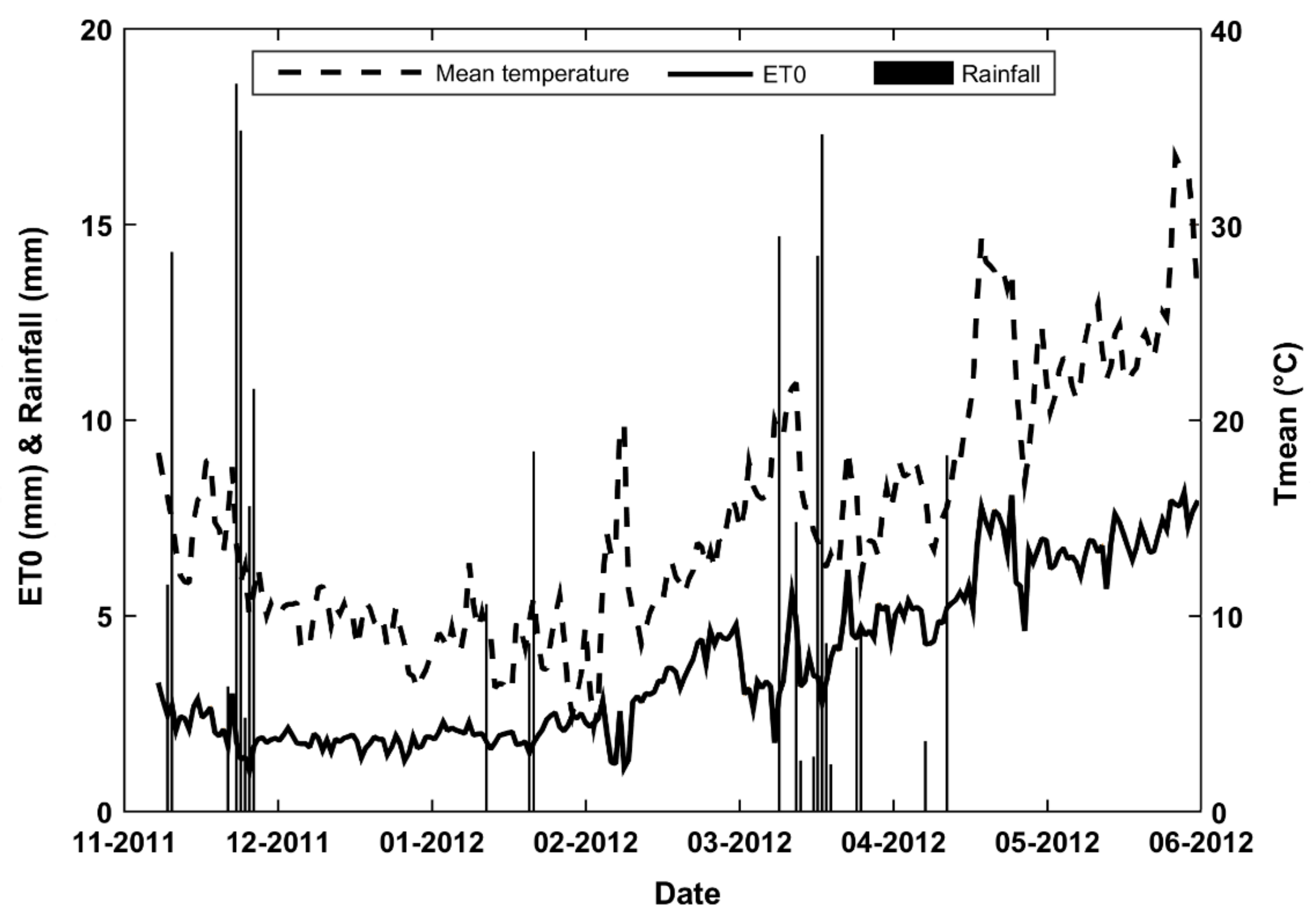
2.3.1. Meteorological Data

To implement and evaluate the proposed approach, we used the meteorological and irrigation data for estimating water requirements, calculating the Ks coefficient, and for estimating the NDVI profile for each spatiotemporal sowing. We also used the Landsat-TM5 image to calculate the observed NDVI profile of each plot. The required data was collected during the 2011–2012 agricultural season in the study area.

The reference evapotranspiration (ET₀) is an indicator of the evaporative demand of the atmosphere and it is calculated using the FAO Penman–Monteith equation [61]. The climatic variables (air temperature and humidity, solar radiation and wind speed) needed to estimate ET₀ and rainfall were measured by an automatic weather station that was installed within the R3 district. More description about this weather station as well as the different sensors used for measuring the different climatic parameters are previously described by [59,64]. Figure 3 shows the daily ET₀, temperature and rainfall calculated during the 2011–2012 agricultural season. The evolution of ET₀ is characteristic of semi-arid continental climate: it is moderate during the autumn (2 to 3 mm/day) and higher in summer (6 to 7 mm/day, in May–June). The annual precipitation is low (equal to 220.7 mm) and irregular and temperature is high in summer (33.5 °C, in June) and low in winter (4.33 °C, in February).

2.3.2. Irrigation Water Supply

The detailed data about effective irrigation schedules (

Table 1. Applied irrigation rounds during the 2011–2012 agricultural season in the study area.

Irrigation Round	Start Date	End Date	Duration (Day)	Applied Water Amounts (mm)
1	3 December 2011	24 December 2011	21	46
2	1 January 2012	21 January 2012	20	52
3	9 February 2012	29 February 2012	20	52
4	1 March 2012	23 March 2012	22	100
5	22 April 2012	4 May 2012	12	24

) at the field scale was time-consuming, and it was surveyed locally in collaboration with the ORMVAH service. The simulations concerned 116 plots which constitute an important global area of about 1260 ha (45% R3 area). Five irrigation rounds for the wheat growing season in 2011–2012 were applied, which durations lasted between 12 and 22 days as presented in Table 1.

2.3.3. Wheat Fields Identification

Land cover mapping was established using a classification method based on NDVI time series obtained from satellite images and was validated by field surveys and data provided by the ORMVAH. In our case, among 18 Landsat images collected during the 2011–2012 wheat season, only 2 images were affected by clouds and were not used in this study. We used 16 Landsat-TM5 images well distributed throughout the agricultural season 2011–2012. Thus, the daily values of the NDVI are easily obtained by linear interpolation [65]. Radiometric calibration and atmospheric corrections were performed on these images based on the reflectance of invariant objects (bare soil, fallows and houses) to provide NDVI time series over the irrigation scheme according to the reported method by [66]. The NDVI profiles obtained for each pixel were used to provide land cover map of the area, identifying the wheat fields concerned by our study, using a decision-tree algorithm based on NDVI thresholds characterizing particular crops phenological aspects [65].

2.3.4. Applied Sowing Dates Identification

To estimate the applied sowing date of each field at the agricultural season 2011–2012, we used the NDVI time series calculated from the collected Landsat-TM5 images. The sowing date is estimated from the emergence date, which is identified when the canopy cover (CC) reaches a value of 0.1 [61]. The values of the canopy cover are estimated from the observed NDVI at the plot level (see Section 2.4). The sowing date is then obtained by subtracting 13 days starting from the emergence date for the case of early sowing and 20 days for the case of late sowing. These values (13 and 20 days) were estimated based on observations monitored in the study area [62,64]. The date of December 20 is commonly considered in our region to distinguish between early and late sowing in accordance with the impact of agro-environmental conditions on wheat growth and development and the farmer’s agricultural practices, particularly the wheat cultivars used [57,62,67].

2.3.5. Irrigation Network Identification

The irrigation network serving the farmer’s fields with water was identified and mapped in a geographic information system (GIS) composed mainly of:

• Canals: line type, characterized by an id number, maximum discharge, the flow direction, the geographic coordinates, the category (primary, secondary or tertiary) and plots that are fed;
• Water intakes: point type, representing the devices that supply a plot or a set of plots. Each intake is characterized by an id number, the geographical coordinates, the maximum discharge, the number of plots it supply, the opening and closing times and the id number of the canal to which it is linked;
• Plots: polygon type, characterized by an id number, the farmer’s name, the type of crop, the id number of the canal and the water intake, the date of sowing, the overall area, the irrigated area and the effective irrigation water applied in 2011–2012 season (in terms of time and quantity).

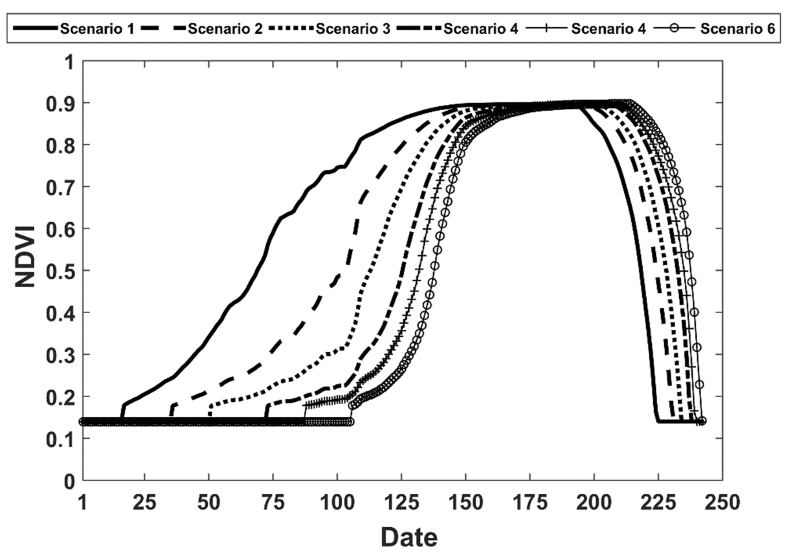
2.4. NDVI Profiles Simulation

For the simulation of the NDVI profiles for each irrigated plot according to the adopted sowing date, we first applied the equations defined by the FAO crop growth simulation model “AquaCrop” [68,69] to generate the green canopy cover profile along the wheat season.

The canopy development is simulated by Equations (1)–(3):

• Exponential growth (CC <= CC_x/2):

  $$\mathrm{CC}={\mathrm{CC}}_0{\mathrm{e}}^{\mathrm{tCGC}}$$

  (1)
• Exponential decay (CC > CC_x/2):

  $$\mathrm{CC}={\mathrm{CC}}_{\mathrm{x}}-0.25\frac{{\left({\mathrm{CC}}_{\mathrm{x}}\right)}^2}{{\mathrm{CC}}_0}{\mathrm{e}}^{-\mathrm{tCGC}}$$

  (2)
• The decline in green crop canopy is described by:

  $$\mathrm{CC}={\mathrm{CC}}_{\mathrm{x}}\left[1-0.05\left({\mathrm{e}}^{\frac{3.33\mathrm{CDC}}{{\mathrm{CC}}_{\mathrm{x}}+2.29}\mathrm{t}}-1\right)\right]$$

  (3)

  where CC is the canopy cover at time t (%), CC₀ is the initial canopy cover at t = 0 (%), CC_x is the maximum canopy cover at the start of senescence (t = 0), CGC is the canopy growth coefficient (% or cumulative growing degree days), CDC is the canopy decline coefficient (% or cumulative growing degree days), and t is time (days or cumulative growing degree days).

The canopy cover profile is then described by the four parameters: CC₀, CGC, CC_x and CDC. CC₀, CGC and CC_x determine the time required to reach maximum canopy cover, whereas the canopy decline coefficient CDC determines the rate of the green canopy decline in the late season. For our proposed approach, we used the calibrated values of CC₀, CGC, CC_x and CDC obtained by [36] for wheat crop grown in the study area (R3) (

Table 2. Parameters values used to calculate the canopy cover.

	Early Sowing	Late Sowing
CC0	4.5	3.83
CCX	89.33	81.33
CGC	0.0089	0.0089
CDC	0.145	0.145

).

Once the canopy cover profiles generated, the NDVI profiles were obtained using the relationship between NDVI and the canopy cover (CC) previously established by [70] for the wheat in R3 area (Equation (4)):

$$\mathrm{NDVI}=\left(\mathrm{CC}+1.18\times {\mathrm{NDVI}}_{\min }\right)/1.18$$

(4)

with NDVI_min = 0.14 as the minimum value of NDVI, associated with bare soil and dense vegetation in our study area [70].

In the proposed approach, the generated NDVI profiles are used in the optimization process, considering that the available water is the only factor limiting the optimal crop growth.

The values of the canopy cover (CC) are also used to calculate the stopping irrigation window at each sowing scenario (see Section 3.2). We consider that the irrigation of a plot must be stopped once the CC reaches a value equal to the half of the maximum canopy cover at the start of senescence (i.e., CC_x/2). In the proposed approach, the optimization process (see Section 2.7) has been defined such that the irrigation window never overlaps the stopping irrigation window.

2.5. Spatialized Estimates of Crop Water Needs and Water Stress Level

In order to predict the amount of irrigation water needed by each plot, we used the soil water balance approach based on the FAO-56 dual crop coefficient model, which is widely used and allows simple and robust modeling [39,61,70,71]. This approach quantifies the crop evapotranspiration under standard conditions (ET_c) as the product of the reference evapotranspiration (ET₀) and a crop coefficient that account separately for the crop transpiration K_cb (basal crop coefficient) and for the soil evaporation K_e (soil evaporation coefficient). Additionally, in order to account for the level of the crop water stress to decide when to trigger irrigation, we evaluated the water stress coefficient (K_s). Thus, the actual evapotranspiration (ET) is given by Equation (5):

$$\mathrm{ET} = \left({\mathrm{K}}_{\mathrm{cb}}{\mathrm{K}}_{\mathrm{s}}+{\mathrm{K}}_{\mathrm{e}}\right)\times {\mathrm{ET}}_0$$

(5)

where K_cb and K_e are derived from NDVI observations using Equations (5) and (6) [64,70]:

K_cb = 1.64 NDVI − 0.2296

(6)

K_e = (0.2 (1 − CC))

(7)

where CC is the canopy cover calculated with Equation (4).

The water stress coefficient is given by Equation (8) [61]:

$${\mathrm{K}}_{\mathrm{s}}=\frac{\mathrm{TAW}-{\mathrm{D}}_{\mathrm{r}}}{\mathrm{TAW}-\mathrm{RAW}}\le 1 \mathrm{when} {\mathrm{D}}_{\mathrm{r}}>\mathrm{RAW}$$

(8)

where Dr is the root zone depletion in (mm) and RAW is the readily available soil water in the root zone (mm).

When Dr ≤ RAW, Ks is equal to 1. TAW is the total available soil water in the root zone [mm], expressed by the difference between the water content at field capacity and wilting point (Equation (9)):

$$\mathrm{TAW}=1000\left({\theta }_{\mathrm{FC}}-{\theta }_{\mathrm{WP}}\right){\mathrm{Z}}_{\mathrm{r}}$$

(9)

where ${\theta }_{\mathrm{FC}}$ is the water content at field capacity in (m³ m⁻³), ${\theta }_{\mathrm{WP}}$ is the water content at wilting point in [m³/m³] and Zr the rooting depth in (m) which varies according to the plant growth stages.

RAW is expressed by Equation (10):

$$\mathrm{RAW}=\rho \mathrm{TAW}$$

(10)

where $\rho$ is the average fraction of TAW that a crop can extract from the root zone without suffering water stress (0–1).

The daily soil water balance, expressed in terms of depletion at the end of the day by Equation (11):

D_r,i = D_r,i−1 − (P − RO)_i − I_i − CR_i + ET_c,i + DP_i

(11)

where D_r,i−1 and D_r,i are respectively the root zone depletion at the end of day i − 1 and i (mm), and Pi is the precipitation, RO_i is the runoff, Ii is the net irrigation depth, CR_i is the capillary rise from the groundwater table, ET_c,i is the crop evapotranspiration, and DP_i is the water loss out of the root zone by deep percolation on day i (mm).

2.6. Grain Yield Estimation

2.6.1. NDVI-Based Approach

Ref. [72] is one of the first to examine the relationships between developed NDVI and the biophysical parameters of vegetation cover. Many subsequent studies have been based on the ability of vegetation indices to predict agricultural production and yield [73,74,75]. Among these indices, NDVI has been used successfully to predict wheat yields in Morocco both at regional and national levels [76]. Thus, in this study, we considered the work carried out by [74] who established an operational method for forecasting crop yields based on NDVI data. It consists in defining a linear relationship between wheat yield and the 10-day spatial accumulation of NDVI values during critical phases of crop development. This approach was tested and validated using data of real grain yield of winter wheat obtained on ten fields of the study area during the 2002–2003 agricultural season [62,77,78]. Thus, for the estimation of wheat yield, we used a relationship developed and validated by [78] which considers the climatic and phenological characteristics of winter wheat in the Haouz plain and showed that the last 10 days of March present the best correlation between yield and ten-day NDVI (Equation (12)). This is consistent with the phenological calendar of winter wheat in the Haouz region. During the second half of March, the wheat is fully developed, photo-synthetically active and the crop reaches the grain filling stage [67,77,79].

$$\mathrm{Yield}=1.79\times \sum \mathrm{NDVI}+8.62$$

(12)

2.6.2. AquaCrop-Based Approach

The AquaCrop is a water-driven model developed by the Land and Water Division of the Food and Agriculture Organization of the United Nations (FAO). In this model, transpiration (Tr) is calculated first based on a water balance model and then converted into biomass (B) using a conservative crop specific parameter called water productivity (WP) (Equation (13)). The biomass is then translated into grain yield (Y) using harvest index (HI) (Equation (14)) [69,80]. To run simulations, AquaCrop requires inputs of climate data, crop characteristics, soil characteristics and description of management practices [69]. A detailed description of the AquaCrop model is available in [69,80].

Ref. [36] calibrated and validated the AquaCrop model for irrigated wheat in our study area, on the basis of a comparison between measurements and the model estimations. Ref. [15] used AquaCrop model to evaluate the impact of climate change on the wheat grain yield and water requirement in our study area. In this study, to simulate wheat grain yield, AquaCrop (v.6.1) was used, with calibrated parameters reported in [36].

$$\mathrm{B}=\mathrm{WP}.\sum \mathrm{Tr}$$

(13)

where B is the above ground biomass (kg/m²), WP is the normalized water productivity (kg·m⁻²) and Tr is the crop transpiration (mm).

$$\mathrm{Y}=\mathrm{B}.\mathrm{HI}$$

(14)

where Y is the grain yield (kg/m²), B is the total ground biomass (kg/m²) and HI is the harvest index (%).

2.7. The Optimization Methodology

The optimization problem presented in this study is considered as a nesting of three sub-problems: sequential scheduling, linear optimization and traveling salesman type. The problem of scheduling displacements from one water intake to another to serve all the plots is equivalent to the travelling salesman problem, where we seek the best path to move from a starting point to a destination point. In our case, we have other problems to solve, such as the management of flow variations and the management of crop water requirements and water stress. This justifies that the studied scheduling problem is particularly difficult to formulate in a way to be able to solve it using an exact method or by an algorithm of the graph theory. Thus, the approach adopted in this work is based on a CMA-ES algorithm belonging to the family of meta-heuristic algorithms inspired by the theory of evolution.

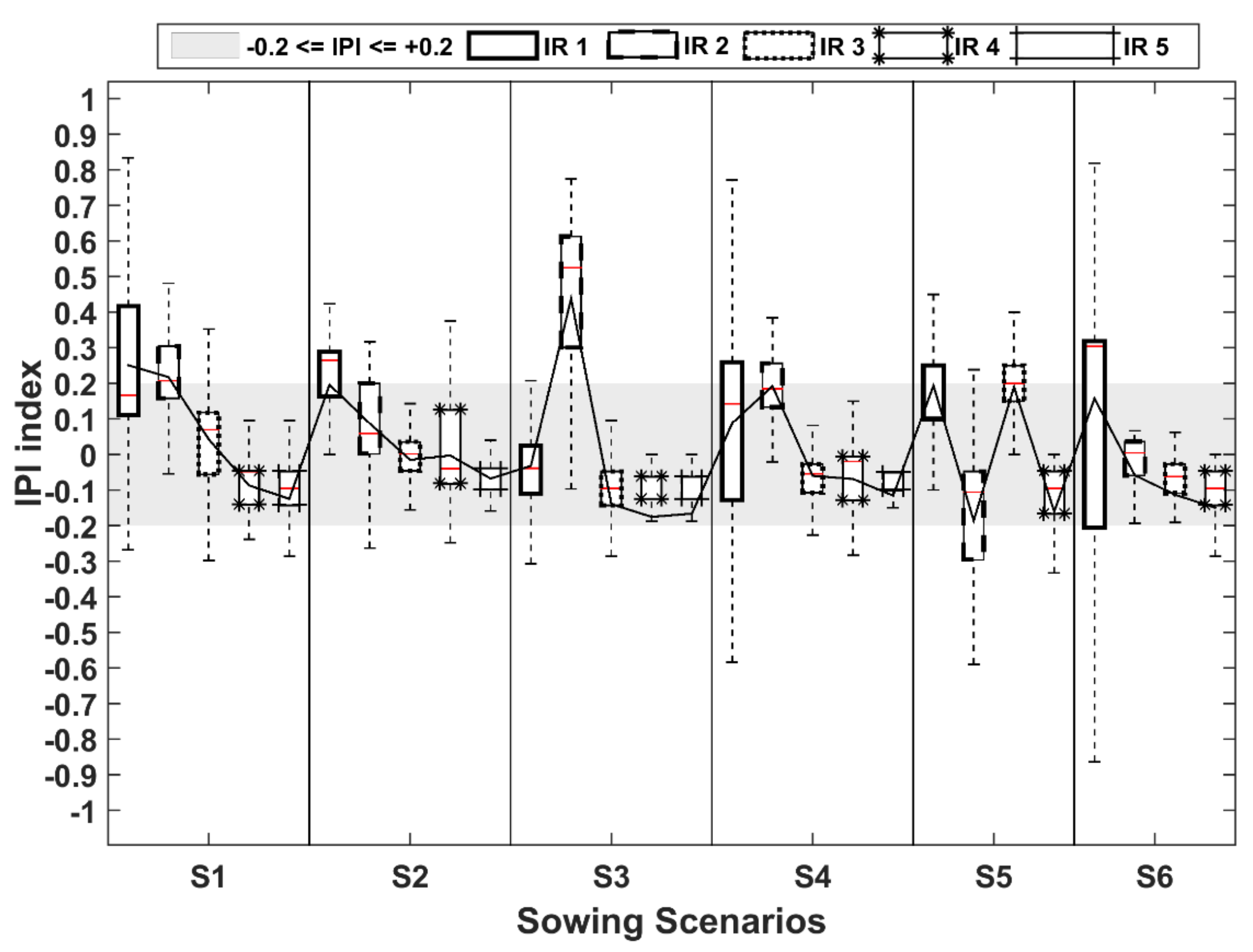
2.7.1. Irrigation Priority Index (IPI)

The optimization of the irrigation schedules over the irrigation scheme in our approach is based on the Irrigation Priority Index (IPI) (Equation (15)), previously developed by [56], which characterizes the irrigation priority of a plot during each irrigation round. The IPI index is calculated for each plot i according to two main terms: a first term that measures the level of water stress of the field j relatively to all the plots concerned by the irrigation round, which allows to quantify the water needs just before the start of the irrigation round and a second term that measures the duration (in days) between the starting date of the irrigation round and the date the plot i receives water. The proposed expression for the IPI is given as follows:

$${\mathrm{IPI}}_{\mathrm{i}}=\frac{{{\mathrm{K}}_{\mathrm{s}}}_{\mathrm{i}}-{{\mathrm{K}}_{\mathrm{s}}}_{\min }}{{{\mathrm{K}}_{\mathrm{s}}}_{\max }-{{\mathrm{K}}_{\mathrm{s}}}_{\min }}-\frac{{\delta t}_{\mathrm{i}}}{\mathrm{T}}$$

(15)

where ${{\mathrm{K}}_{\mathrm{s}}}_{\mathrm{i}}$ is the water stress at the beginning of the irrigation round, and ${{\mathrm{K}}_{\mathrm{s}}}_{\min }$ and ${{\mathrm{K}}_{\mathrm{s}}}_{\max }$ are the spatial minimum and maximum of the K_s map that represent the most and less stressed plots, respectively. $\delta t_{\mathrm{i}}$ the time delay (in days) between the beginning time of the irrigation round and the irrigation time of plot i and T the duration of the irrigation round. Values of $\delta t_{\mathrm{i}}$ range between 0 and T and are chosen as the decision variables of the optimization process.

The proposed IPI equation limits its values between −1 and +1. An IPI = −1 corresponds to an extreme late irrigation (the most stressed plots irrigated the last day of the irrigation round); IPI = +1 corresponds to an extreme early irrigation (the less stressed plot irrigated in advance). Contrarily, an IPI = 0 corresponds to the plots irrigated at the appropriate time, which means a reasonable tradeoff between the water stress level and the irrigation time. Thus, values of IPI close to 0, on both sides, are considered as an indicator of optimal irrigation distribution during an irrigation round.

2.7.2. Sowing Date Optimization

The spatiotemporal sowing date optimization approach is defined in two steps: (1) the choice of a sowing scenario and (2) the development of a first optimal spatiotemporal sowing date distribution according to the chosen scenario. The optimization of this distribution is based on the constraints of the gravity irrigation network as well as on the available water resources at the beginning of the agricultural season. For the resolution of this optimization problem, we propose an approach based on the CMA-ES evolutionary strategy algorithm such as:

(a)

Inputs: available water resources, geospatial data and meteorological data;

(b)

Decision variables: the sowing date of each plot. We have 116 plots to be sown, which means 116 decision variables are considered;

(c)

Optimization constraints: we identified five constraints which we present by a decreasing level of priority.

• The capacity constraint: supplies must never exceed the total capacity of the canal. This constraint is expressed by Equations (16) and (17):

  $${\displaystyle \sum _{j=1}^J{Q}_j}\left(\delta t\right)\le \Theta \left(\delta t\right)$$

  (16)

  $${\displaystyle \sum _{i,j=1}^{I,J}{q}_{ij}}\left(\delta t\right)\le Q_j\left(\delta t\right)$$

  (17)

  where $\theta$, $Q$ and $q$ are respectively the discharge of the primary, secondary and tertiary canals (in m³/s), i and j are respectively the tertiary and secondary canals’ number, opened at the same time;
• The interval constraint: all the irrigation tasks must be scheduled within the specified irrigation round interval, expressed by Equations (18) and (19):

  $$\delta t_{start}\le \delta t_i\le E$$

  (18)

  $$\delta t_i+D_i\le E$$

  (19)

  where $\delta t_{start}$ is the starting date of the irrigation round; $\delta t_i$ the opening time scheduled for canal i; E the allowed duration of the irrigation round, and Di the irrigation duration scheduled for the canal I;
• The overlap constraint: all the practical actions must be applied dependably (not simultaneously), considering the geographical distance between water intakes and the irrigation time span required for each plot supplied by the same canal;
• The traveling time: the time required for the operator to travel from one canal gate to another to start/stop an irrigation which depends on the distance between canals that can be significant. This time is calculated linearly based on the spatial distance between two intakes and assuming a moving speed of 30 km/h;
• The daily working time of operators: each scheduled task (start/stop an irrigation) must be scheduled within the specified working time that is between 8:00 h and 18:00 h;

(d)

The objective function: the first objective function aims to propose the best spatiotemporal sowing distribution which minimize the gravity irrigation network constraints by exploring the space of decision variables in an efficient manner. In case the constraints are not met, we adopt the penalty method by adding penalty function. Thus, the first objective function is defined by Equation (20):

$$F_1={\displaystyle \sum _{j=1}^5{r}_j{P}_j}$$

(20)

where r_j is the weight associated to each constraint j, and P_j the corresponding penalty expressed by Equation (21):

$$P_j={\displaystyle \sum }_{k=1}^N{\vartheta }_{j,k}$$

(21)

where N is the total number of plots to be irrigated and ${\vartheta }_{j,k}=0$ if the task is satisfying the constraints, ${\vartheta }_{j,k}=1$ otherwise.

2.7.3. Irrigation Scheduling Optimization

As previously mentioned, the simulation of the optimal spatiotemporal distribution of irrigation dates at the start of each irrigation round is based on the water stress coefficient level (K_s), while considering the irrigation network constraints. For that, we consider that the best distribution is the one that minimizes the IPI index (in terms of absolute value). Thus, for the resolution of this second optimization problem, we applied the CMA-ES algorithm, such as:

(a)

Inputs: available water resources, geospatial data, meteorological data, soil proprieties, NDVI profiles, and K_s;

(b)

Decision variables: During each irrigation round, two types of decisions must be made: when to irrigate the plots and in what order (i.e., the sequence and scheduling of the irrigations). The answer to these two questions is integrated into a single decision variable that consists of defining the start date to irrigate each plot (the stopping date is calculated based on the water amount to be supplied to a plot given the calculated irrigation duration and the constant flow rate of the tertiary canal). The stating date to irrigate the plots can therefore be considered as the only decision variables in the optimization process. In this work, 116 plots are scheduled, which means that 116 decision variables are considered during the optimization process while considering the constraints related to the irrigation network;

(c)

Optimization constraints: the same as the first optimization (i.e., irrigation network constraints);

(d)

The objective function: the second objective function aims to propose the best spatiotemporal irrigation distribution, which minimize the IPI index and the gravity irrigation network constraints. Thus, the second objective function is defined by Equation (22):

$$F_2={\displaystyle \sum }_{k=1}^N{\left({\mathrm{IPI}}_k\right)}^2+F_1$$

(22)

where k is the canal index and N is the total number of plots to be irrigated.

This optimization allows us to define the optimal opening dates of each canal. Then, to calculate the date to irrigate plots fed by a same canal having limited flow, we applied the shortest job first (SJF) non-preemptive scheduling algorithm [81], which is usually used for scheduling processes. In this algorithm, the process having the smallest value of K_s coefficient is chosen for the next execution, which means that we first begin with the irrigation of the most stressed plots (depending on the canal flow rate), which imply to minimize the level of water stress within the block of plots irrigated by the same canal.

The irrigation duration of each plot is calculated according to Equation (23):

$$\mathrm{Duration} \left(\mathrm{h}\right)=\left(\mathrm{water} \mathrm{rate} \left(\frac{{\mathrm{m}}^3}{\mathrm{ha}}\right)\times \mathrm{area}\left(\mathrm{ha}\right)\right)/ \mathrm{flow}\left({\mathrm{m}}^3/\mathrm{h}\right)$$

(23)

where flow is the maximum canal discharge that should not be exceeded. It depends on the canal capacity, a design characteristic which is equal to 90 L, 60 L, or 30 L/s in our irrigation network. Thus:

• if capacity = 30 L/s: flow = 0.03 × 3600 = 108 m³/h;
• if capacity = 60 L/s: flow = 0.06 × 3600 = 216 m³/h;
• if capacity = 90 L/s: flow = 0.09 × 3600 = 324 m³/h.

3. Results

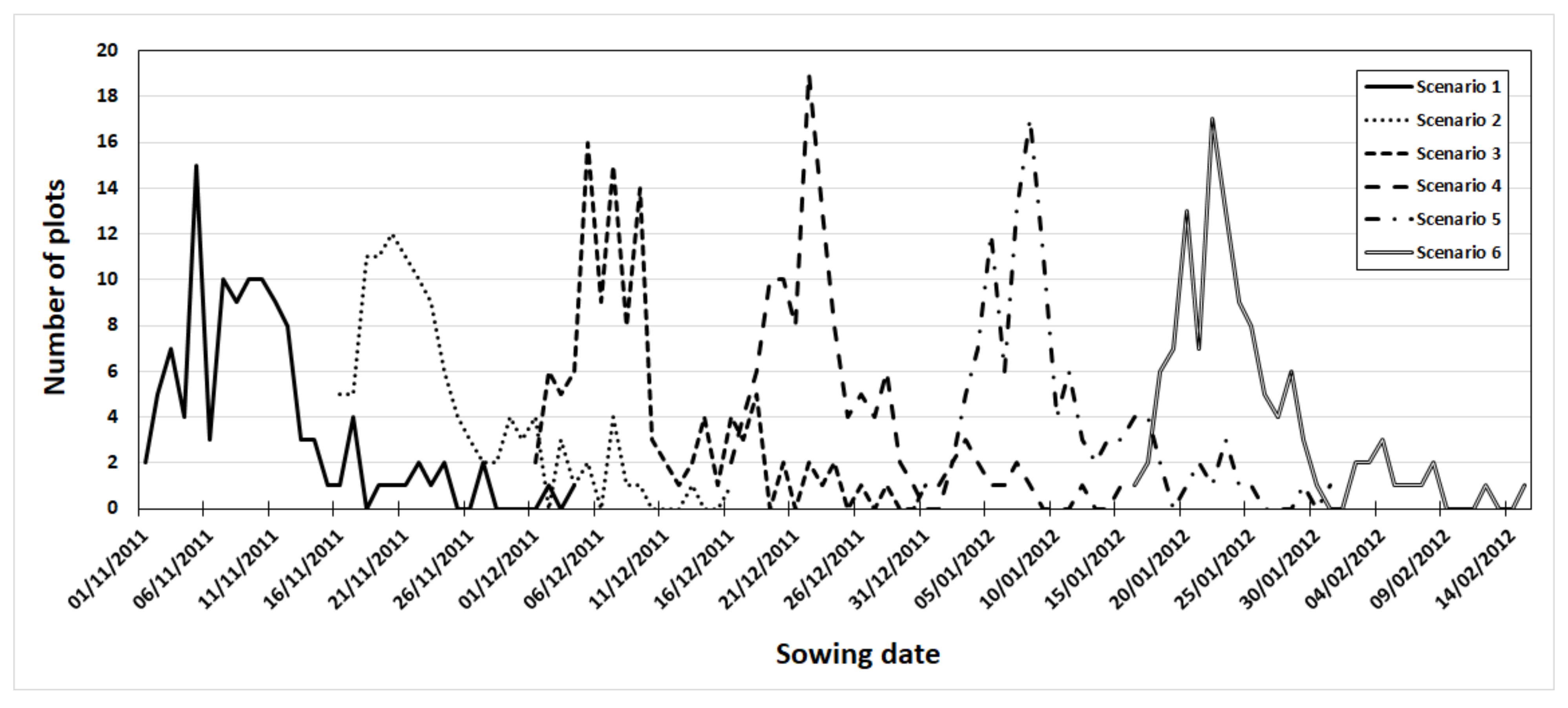
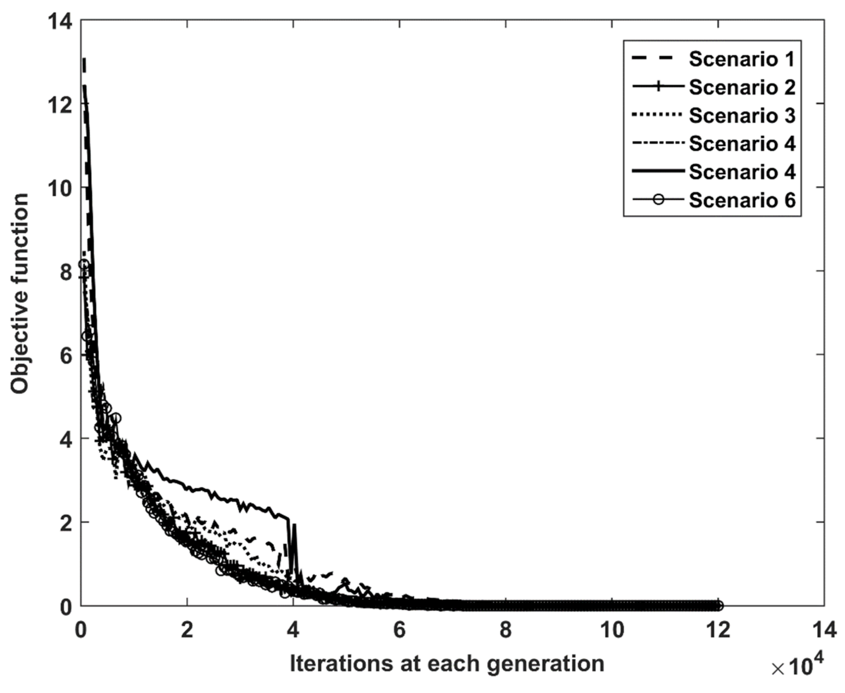
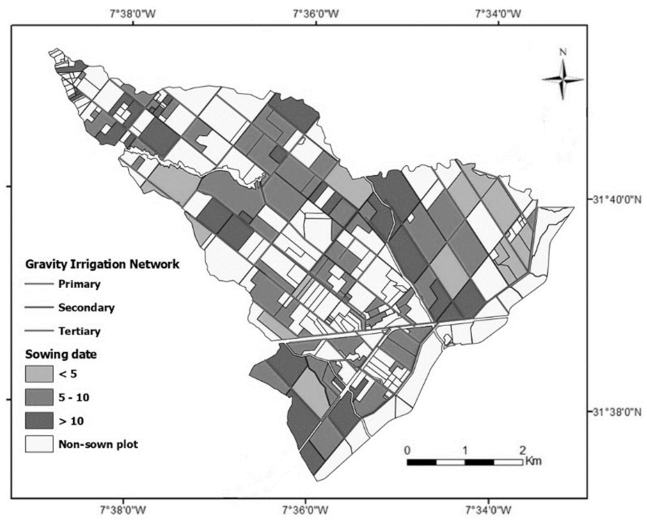
3.1. Optimization of the Spatiotemporal Sowing Date Distribution

The first step of our proposed approach is the optimization of the spatiotemporal distribution of the sowing dates. Six sowing scenarios with different starting date were simulated. The results of this optimization for each sowing scenario are presented in Figure 4. This figure shows practically a similar optimal distribution of the sowing dates from one scenario to another attributed to the fact that this optimization is based on the same inputs data and the same irrigation network constraints, only the initial individuals corresponding to the decision variables (distribution of the sowing dates) in our CMA-ES optimization algorithm change. These latter does not affect the optimal sowing distribution from one scenario to another because we start with a random initial individuals and then during the first iterations of the optimization process, the exploration of the control parameters (decision variables) is weak (Figure 5), which implies the adaptation of the covariance by the CMA-ES algorithm through enlarging the range of these parameters and then refining search of parameters to obtain a rapid reduction of the objective function. The convergence of this function for each sowing date scenario is presented in Figure 5.

We also notice in Figure 4, that for the different scenarios, a high number of plots are sown between the 5th and the 10th day (counting from the starting date of each sowing scenario). This is attributed to the fact that our optimization approach maximizes the number of plots sown at the beginning, in such way that we can irrigate the same number of plots at the same time when starting an irrigation round. Thus, the sowing date of the remaining plots (which are no longer numerous) is defined based on the irrigation duration of the first group of sown plots which will be irrigated by the same canal (to not exceed the maximum flow rate). This method was applied to lead to an irrigation schedule that follows the same sowing schedule in order to ensure a good balance between the water stress level and the irrigation date. An example of the sowing date distribution (first sowing scenario) is presented in Figure 6. It can be seen that a high number of plots (54%) are sown between the 5th and the 10th day.

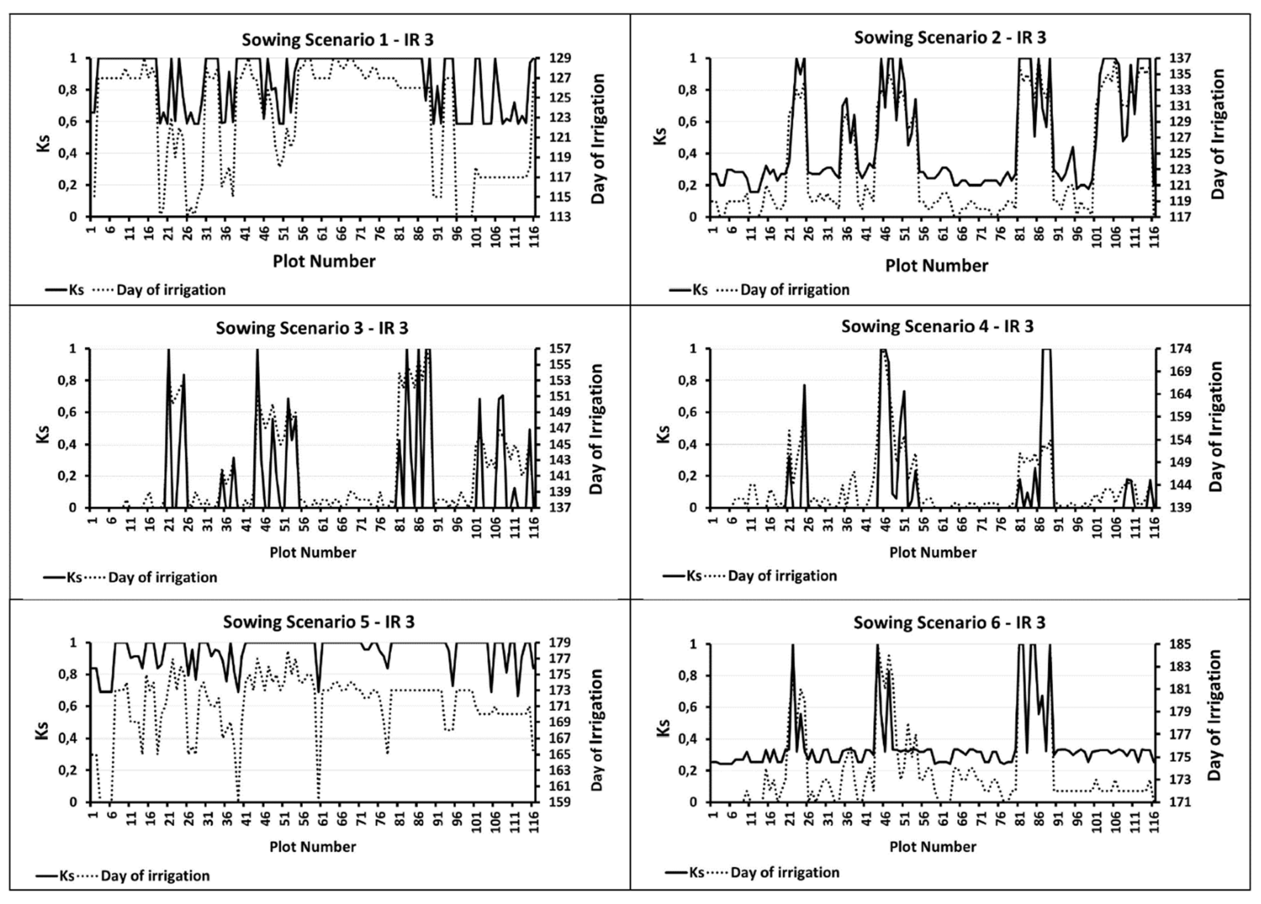
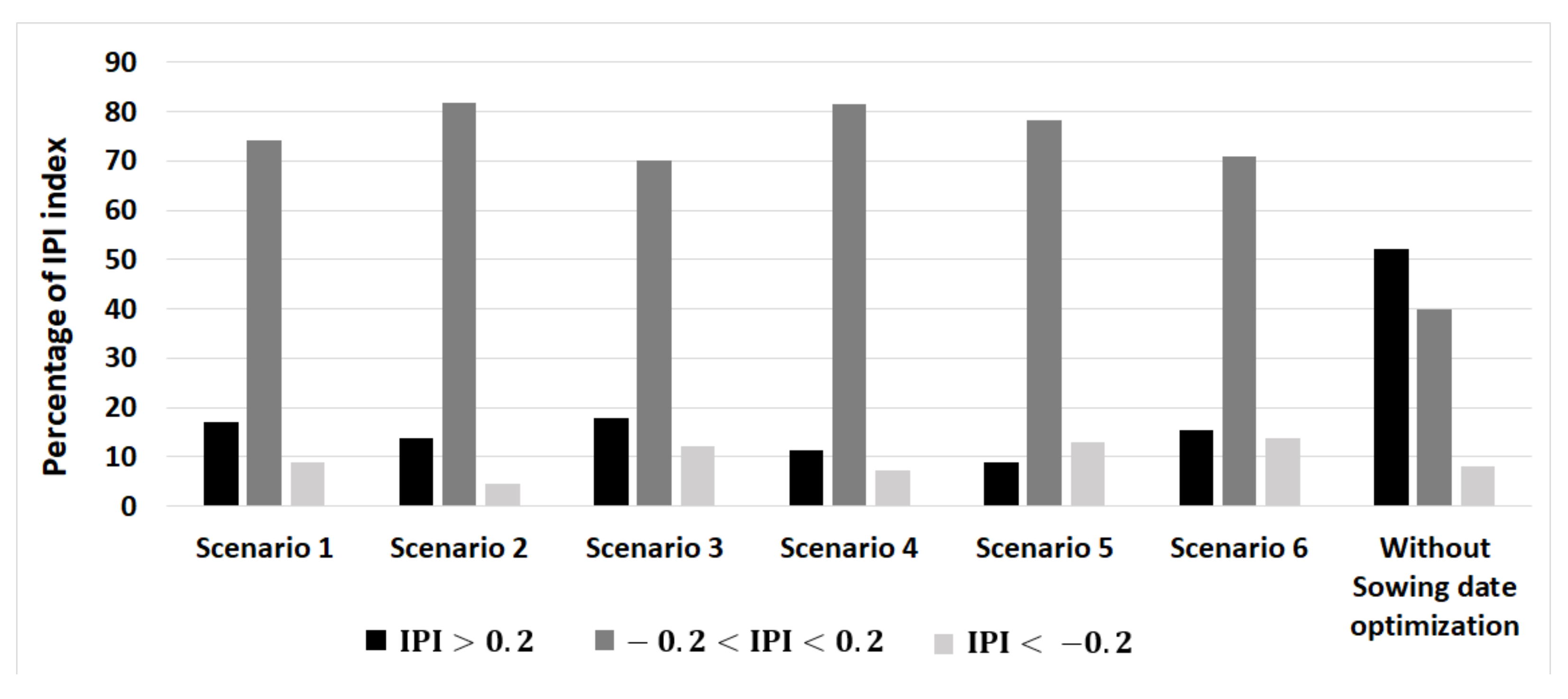
3.2. Effect of Sowing Date Optimization on Wheat Growth and Irrigation Schedules

Once the distribution of sowing dates was optimized, the NDVI profiles were generated for each plot according to its sowing date using Equations (1)–(4). Figure 7 presents an example of the difference in NDVI profiles for a single plot (with area = 9.72 ha), by varying sowing date window from one scenario to another. This figure shows clearly that the duration of wheat season decreases from early to late sowing (from 208 to 137 days), which affects the crop development and growth [15,36]. The NDVI profiles of all plots in the study area were then used to calculate the water stress coefficient Ks, initially between the sowing date and the starting date of the first irrigation round, and between the different irrigation rounds, according to the approach presented in the Section 2.2. An example of KS maps at the start of the third irrigation round for the first sowing scenario (early sowing) and the sixth sowing scenario (late sowing) is displayed in Figure 8. The spatial heterogeneity of the Ks values between plots irrigated by the same canal and the effect of the spatiotemporal distribution of sowing dates on water stress are clearly observed. This heterogeneity is also illustrated in Figure 9, which presents the Ks values for each plot at the starting of the third irrigation round for each sowing scenario. We also notice in this figure that the optimal irrigation date follows the evolution of the Ks level, i.e., the most stressed plots are irrigated first and the least stressed are irrigated last.

The next step is the irrigation scheduling optimization process based on the IPI index derived from Ks stress coefficient maps elaborated at the beginning of each irrigation round. An irrigation round is decided when the K_s reaches a value less than 0.7 at most for 5% of the total cultivated plots.

The results of IPI optimization at plot scale for each sowing scenario are presented in Figure 10. It can be seen that for almost all sowing scenarios, the majority of plots is irrigated at the appropriate time considering their water stress level, which illustrates the performance and the efficiency of the optimization approach. The optimized sowing distribution and irrigation schedules at the plot scale for each scenario leads to a high range of plots irrigated on a favorable time for most irrigation rounds (an average of 76.17% of plots with −0.2 =< IPI <= +0.2) and a low range of plots irrigated early (an average of 14.19% of plots with IPI > +0.2) or lately (an average of 9.64% of plots with IPI < −0.2). Based on the obtained results, we can conclude that the 1st and the 2nd sowing scenarios (starting dates 1 November 2011 and 16 November 2011, respectively) are the best for a better optimization of the IPI indices and then a good irrigation scheduling optimization [56]. By comparing with the other four scenarios, these two early sowing scenarios have a high percentage of plots irrigated at the appropriate time (between 42.2% and 97.4%) and a low percentage of late irrigated plots (between 0.86% and 11.2%). The number of irrigation rounds can be reduced from five (for first to fourth scenario) to four (for both fifth and sixth scenarios).

Conversely,

Table 3. Optimized irrigation windows, sowing windows, stopping irrigation window, number and mean duration of irrigation round (IR) and the mean gap between two successive irrigation rounds.

Scenario	Gap between IR (Day)	Mean IR Duration (Day)	Number of IR	All Irrigations Window	Stopping Irrigation Window	Sowing Window
1	16	18	5	[14 December 2011–19 May 2012]	[30 May 2012– 12 June 2012]	[1 November 2011– 4 December 2011]
2	14	21	5	[15 December 2011–29 May 2012]	[7 June 2012– 17 June 2012]	[16 November 2011– 16 December 2011]
3	18	18	5	[30 December 2011–9 June 2012]	[13 June 2012– 25 June 2012]	[1 December 2011–31 December 2011]
4	14	19	5	[14 January 2012– 13 June 2012]	[17 June 2012– 29 June 2012]	[16 December 2011–15 January 2012]
5	13	19	4	[7 February 2012–4 June 2012]	[20 June 2012– 3 July 2012]	[1 January 2012– 31 January 2012]
6	16	19	4	[14 February 2012–17 June 2012]	[23 June 2012– 7 July 2012]	[16 January 2012– 15 February 2012]
Observed irrigation	15	19	5	[3 December 2011–4 May 2012]	[7 June 2012– 25 June 2012]	[16 November 2011–31 January 2012]

presents for the six scenarios the optimized irrigation and sowing windows and the simulated windows to stop irrigation rounds. The results showed a clear impact of the sowing window on the irrigation schedules during the agricultural season: (1) irrigation window is delayed depending on the sowing window, (2) the gap between successive irrigation rounds ranges from 13 to 16 days, the duration of the rounds ranges between 18 and 21 days and the number of irrigation rounds can be minimized when sowing dates are delayed (from five to four). The obtained values of the gap between two successive rounds, the duration and the number of irrigation rounds are consistent with the observed ones at the agricultural season 2011–2012.

Additionally, to evaluate the impact of the sowing date’s optimization on irrigation scheduling, we compared the results of the IPI index distribution obtained by our proposed approach, with the results of a previous study conducted on the same irrigation district [56], but without optimizing the sowing date (i.e., using the applied sowing date at the 2011–2012 agricultural season). The comparison concerned only the third irrigation round of 2011–2012 agricultural season. Three classes (late irrigation, early irrigation and optimal irrigation) of IPI index distribution are presented in Figure 11, for each sowing scenario and compared with the IPI index distribution without sowing dates optimization (from the previous study). We notice that the proposed optimization approach greatly improves the number of plots irrigated at the appropriate time (optimal IPI increase from 40% without sowing date optimization to 82% with sowing optimization according to the second sowing scenario).

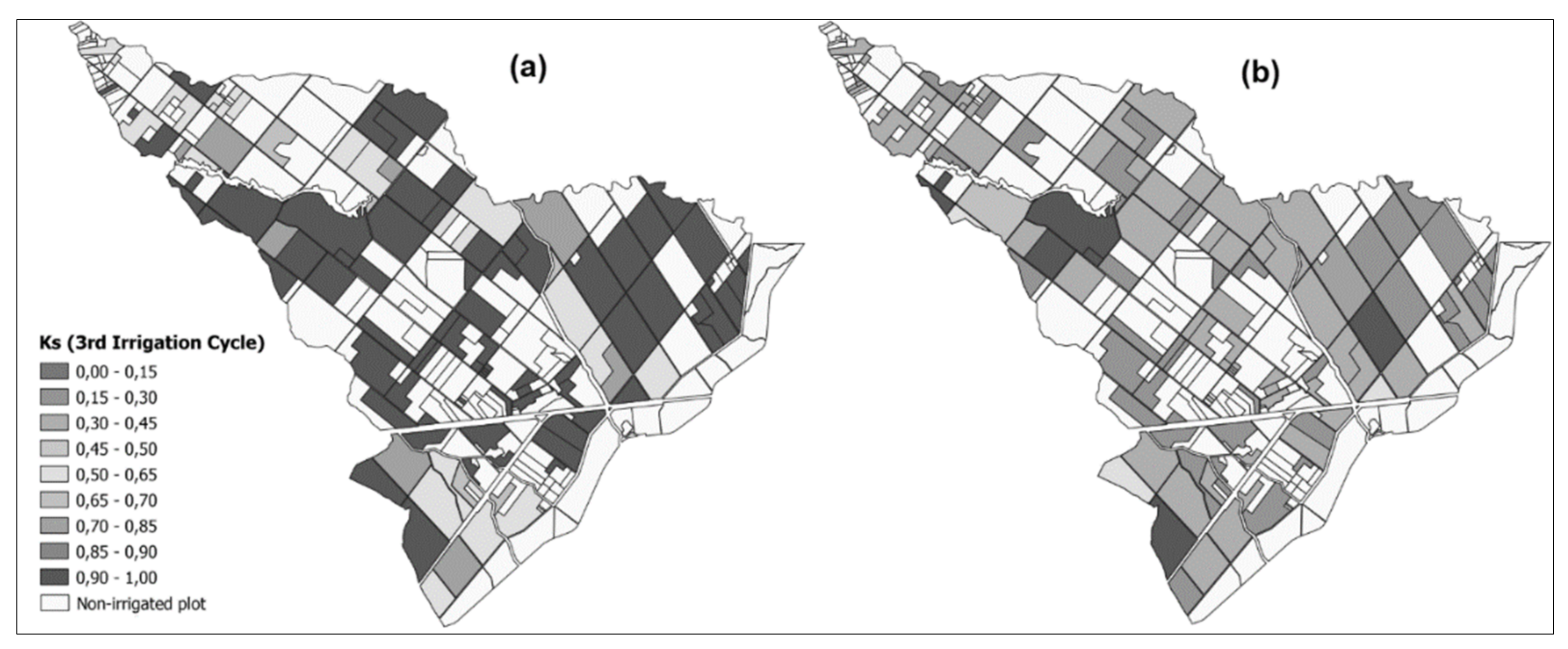
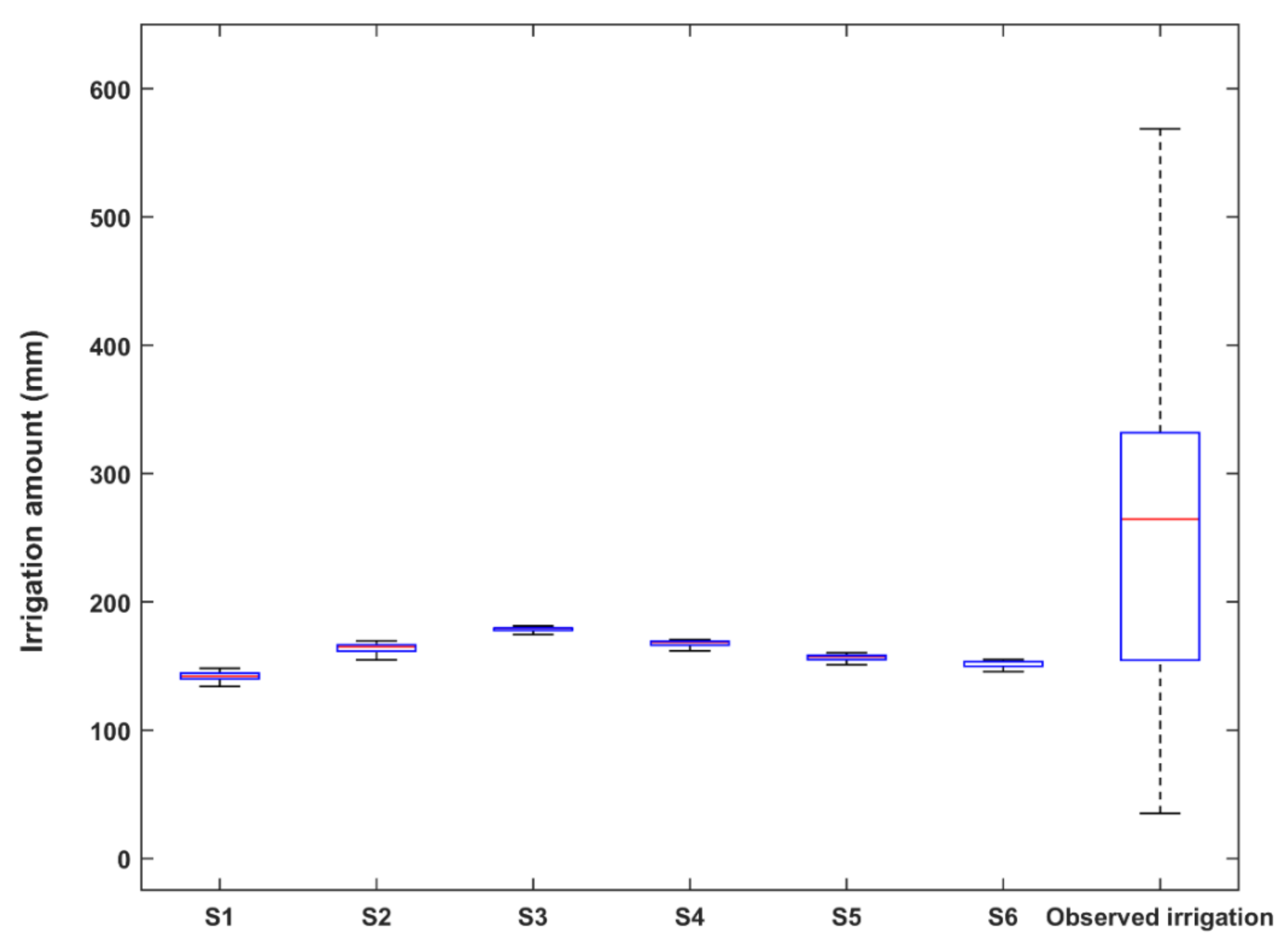
3.3. Effect of Sowing Date Optimization on Water Requirements

To evaluate the effect of sowing optimization on crop water requirement, we compared the simulated water needs at each irrigation round and for each sowing scenario with the applied (observed) irrigation amounts at the agricultural season 2011–2012. The results of this comparison are presented in Figure 12 and summarized in

Table 4. Irrigation water demands (mm) estimated for each irrigation round (IR) compared to the applied irrigations at the 2011–2012 agricultural season.

	IR 1 (mm)	IR 2 (mm)	IR 3 (mm)	IR 4 (mm)	IR 5 (mm)	Total (mm)
1st Sowing Scenario	10	19	30	35	47	141
2nd Sowing Scenario	7	10	33	53	61	164
3rd Sowing Scenario	6	11	32	54	75	178
4th Sowing Scenario	6	11	27	48	75	168
5th Sowing Scenario	8	24	45	79		156
6th Sowing Scenario	4	29	48	72		152
Observed Irrigation	46	52	52	100	24	274

. For all of the scenarios, the overall demand for irrigation water is greatly reduced compared to the observed case. This reduction varied from 48.54% to 35.04% and afterward, to 44.53% for the first, third and sixth scenarios, respectively. The statistical comparison of the performance of these six scenarios, using the Student’s t-test [82], shows that there are two groups of identical scenarios at p > 0.05 (scenarios S1, S5 and S6 as a first group and S2, S3 and S4 as a second group).

Additionally, for all the scenarios, the variation in water demand from one plot to another is largely reduced; it is about ±3 mm for the 1st scenario against ±182 mm for the observed case. This result is important for irrigation equity between fields and between farmers [39].

Table 4 presents the amounts of water applied or simulated at each irrigation round. We notice that they increase from one irrigation round to another depending on the development of the root zone from one stage to another. The low values of the total amount of consumed water resources estimated for the six scenarios vary from 141 to 178 mm, but by adding the rainfall which was taken into account when optimizing the water requirements, we obtain a total volume varying from 362 to 399 mm, and a total amount of 495 mm for the observed irrigation, which is close to the requirements of wheat as defined in other studies [36,38,83].

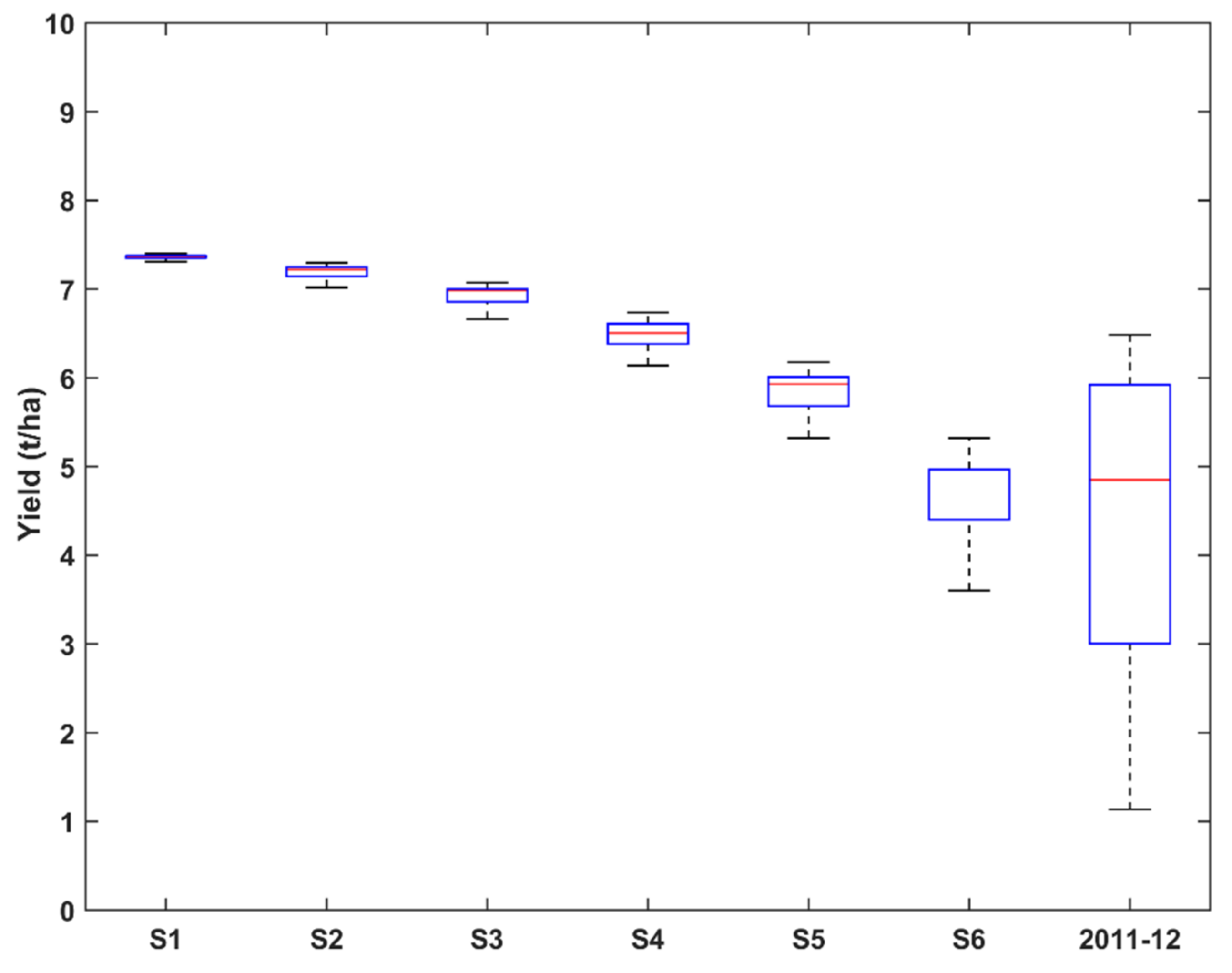
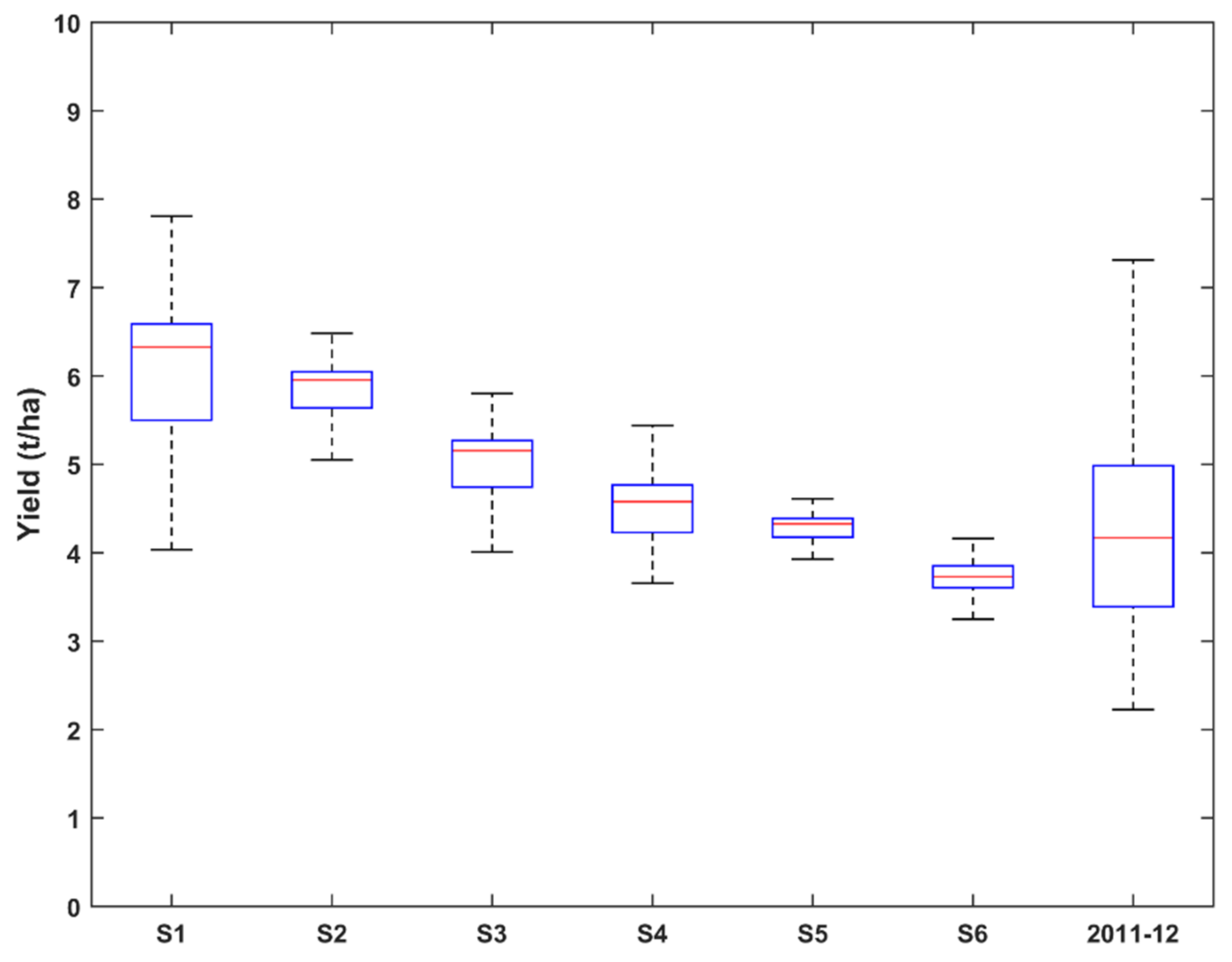
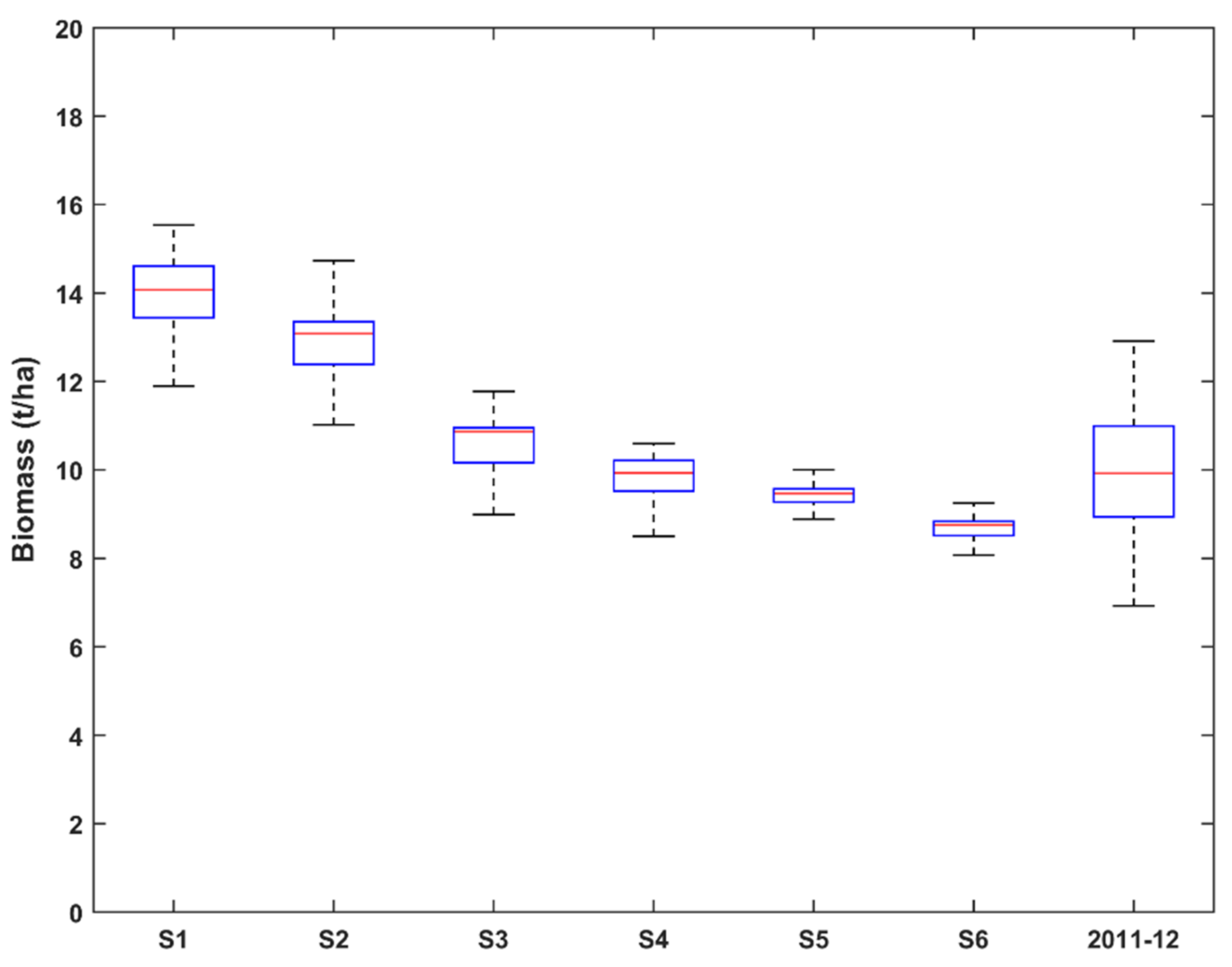
3.4. Effect of Sowing Date Optimization on Wheat Yield

The last objective of our study is to evaluate the impact of the optimized sowing dates and consequently the optimized irrigations on wheat yields (biomass and grain). For this purpose, we compared the simulated wheat yields for each sowing scenario with the estimated ones at the real case. As presented in Section 2.6, two approaches were applied. The first one is based on the NDVI profiles using Equation (12). For each sowing scenario, the NDVI index is calculated based on the sowing dates. We also used the NDVI profiles derived from satellite images which reflect the real crop growth conditions to estimate the real obtained grain yield at the 2011–2012 agricultural season [78]. We remind here that this first approach is used to identify the best spatiotemporal repartition of sowing date corresponding the optimal grain yield. The second approach is based on the AquaCrop model considering crop growth, the sowing dates and the irrigation schedules (times and amounts). In this case, the evaluation of the proposed approach concerns the produced biomass and grain. Figure 13 and Figure 14 present the results of the first and second approach respectively.

The results showed that the wheat yields (grain and biomass) are maximal for the early sowing dates and decrease for the late sowing scenarios. Except for scenario 6, the obtained yields (biomass and grain) are clearly high compared to the observed ones.

Otherwise, for scenario 1, the grain yield obtained by the NDVI-based approach (Figure 13) and by Aquacrop (Figure 14) reach 7.4 and 7.8 t/ha, respectively, and the biomass estimated by Aquacrop is 15.5 t/ha (Figure 15). These yields are comparable to the potential yields that can be obtained under the agro-environmental conditions of our study site [38,62,67]. This excellent result shows the validity of the proposed optimization approach.

The statistical comparison of yields (grain and biomass) estimated for the different scenarios, using the Student’s t-test, shows that overall, the scenarios results, presented in Figure 13, Figure 14 and Figure 15, are significantly different at p ≤ 0.05, except for scenarios S1 and S2 (Figure 13) that are evaluated identical at p > 0.05.

4. Discussion

The main objective of this study is to evaluate the effects of optimized wheat sowing date, based on our proposed approach, on irrigation schedules, water requirements and yield.

Thus, we first illustrated the performance and the efficiency of our optimization approach, by optimizing irrigation schedules based on the IPI index derived from spatialized Ks coefficient, at the beginning of each irrigation round. This optimization leads to a high range of plots irrigated on time for each irrigation round (Figure 10), particularly for the first and the second sowing scenarios (starting dates 1 November 2011 and 16 November 2011, respectively), while promoting early irrigation over late irrigation because it avoids crop water stress and leads to increased yields [62,78]. Then, to evaluate the impact of sowing date’s optimization on irrigation scheduling, we compared the obtained results with another approach based only on IPI index optimization without optimizing the sowing date. Results show that with our proposed approach including sowing date optimization we can reach a high percentage of plots irrigated at the appropriate time (Figure 11). This revealed that the optimization of the spatiotemporal distribution of sowing date over the irrigation scheme has a significant impact on the irrigation schedules and their optimization process, thereby increasing the adequacy of the supply of irrigation supply to meet crop water needs.

Conversely, to evaluate the effect of sowing optimization on crop water requirement, we compared the simulated water needs with the observed irrigation amounts. Results show that with an early sowing dates we can reach a high reduction (up to −40%) of water resources (Table 4), and that with the scenario 3 (stating date 1 December 2011), we have a relatively high demand, compared to the other scenarios, which is justified by the occurrence of the grain maturity stage in April, which is associated with high air temperatures and consequently high evapotranspiration [62]. This situation is much more critical for the three scenarios (4th to 6th), but the relative high air temperatures during all the phenological stages of wheat greatly reduces the crop cycle [15] and therefore a decrease in water demand. However, this climate condition for these three scenarios impacted significantly the wheat yield in biomass and grain [60,63].

The evaluation of the effect of sowing date optimization on wheat yields (biomass and grain) showed that with the early sowing scenarios we can increase the wheat yields compared to the late sowing scenarios (Figure 13). This result is in agreement with previous research results conducted for the wheat crop in the same study area [36,63]. In this semi-arid zone, early sowing allows wheat to have a relatively long cycle allowing crops to absorb a high amount of solar radiation, which consequently leads to a high yield [63,84]. Moreover, late sowing dates correspond to pollination and grain filling stages in April month characterized by high air temperatures. This increases the risk of heat stress, which significantly affects the grain weight and the number of grains per ear [85].

Thus, the promising outputs of this study highlighted the interest of the adoption of the suggested approach by the managers of gravity irrigation schemes as an efficient tool for optimal sowing date shifting and optimal irrigation scheduling, which can be considered as key adaptation strategies to ensure agricultural water sustainability.

5. Conclusions

In order to contribute to the adaptation of agricultural practices to water scarcity conditions and to meet wheat production needs in the context of climate change, the effect of shifting sowing calendars was considered in this study. An approach based on remote sensing and on the CMA-ES evolutionary algorithm was developed to optimize the spatiotemporal sowing date distribution of wheat crop in a large irrigation scheme located in Haouz plain (Morocco), considering the different constraints related to the irrigation network as well as the climatic conditions and available water resources. Different sowing scenarios were simulated to evaluate the performance of our approach and to evaluate the effect of the sowing date optimization on irrigation management and crops yield, using weather data, field data and irrigation practices data collected in the study area during the 2011–2012 agricultural season. The results showed a high efficiency of the proposed approach by increasing yield, reducing irrigation water demand and rationalizing irrigation scheduling, compared to observed data.

Conversely, the simulation results showed a significant impact of the sowing window optimization on the irrigation schedules during the agricultural season, mainly the obtained irrigation windows, the gaps between successive irrigation rounds, and the duration and the number of irrigation rounds.

The effect of sowing optimization on crop water requirement was also evaluated by comparing the estimated water needs derived from crop evapotranspiration (ET_c) with the observed irrigation amounts applied by farmers. Results showed that a reduction of up to −40% of water needs can be achieved. The simulated wheat yields after sowing dates optimization were compared with the estimated ones at the real case by applying two different approaches: NDVI-based approach and AquaCrop model. The results revealed that the early sowing scenarios lead to higher wheat yields compared to the late sowing scenarios for both approaches with a homogeneous distribution over the plots compared to the observed one, which implies a better equity among farmers.

Further simulations and validation in different agricultural seasons and different climate conditions and geographic regions, while considering more complicated cropping patterns, are needed to improve the proposed approach.

References

1. Harbouze, R.; Pellissier, J.-P.; Rolland, J.-P.; Khechimi, W. Rapport de synthèse sur l’agriculture au Maroc. [Research Report] CIHEAM-IAMM. 2019, pp. 104, hal-02137637v2. Available online: https://hal.archives-ouvertes.fr/hal-02137637v2 (accessed on 20 July 2021).
2. Verner, D.; Treguer, D.; Redwood, J.; Christensen, J.; McDonnell, R.; Elbert, C.; Konishi, Y.; Belghazi, S. Climate Variability, Drought, and Drought Management in Morocco’s Agricultural Sector. World Bank, Washington, DC. © World Bank. 2018. Available online: https://openknowledge.worldbank.org/handle/10986/30603 (accessed on 20 July 2021). License: CC BY 3.0 IGO.
3. Trnka, M.; Feng, S.; Semenov, M.A.; Olesen, J.E.; Kersebaum, K.C.; Rötter, R.P.; Semerádová, D.; Klem, K.; Huang, W.; Ruiz-Ramos, M.; et al. Mitigation efforts will not fully alleviate the increase in water scarcity occurrence probability in wheat-producing areas. Sci. Adv. 2019, 5, eaau2406. [Google Scholar] [CrossRef] [Green Version]
4. Le Page, M.; Zribi, M. Analysis and Predictability of Drought In Northwest Africa Using Optical and Microwave Satellite Remote Sensing Products. Sci. Rep. 2019, 9, 1466. [Google Scholar] [CrossRef] [Green Version]
5. IPCC. Annex II: Glossary. In Climate Change 2014: Synthesis Report; Contribution of Working Groups I, II and III to the Fifth Assessment Report of the Intergovernmental Panel on Climate Change, Core Writing Team; Pachauri, R.K., Meyer, L.A., Eds.; IPCC: Geneva, Switzerland, 2014; pp. 117–130. [Google Scholar]
6. Tian, Y.; Zheng, C.; Chen, J.; Chen, C.; Deng, A.; Song, Z.; Zhang, B.; Zhang, W. Climatic Warming Increases Winter Wheat Yield but Reduces Grain Nitrogen Concentration in East China. PLoS ONE 2014, 9, e95108. [Google Scholar] [CrossRef] [Green Version]
7. Porter, J.R.; Semenov, M. Crop responses to climatic variation. Philos. Trans. R. Soc. B Biol. Sci. 2005, 360, 2021–2035. [Google Scholar] [CrossRef]
8. Lobell, D.B.; Burke, M.B.; Tebaldi, C.; Mastrandrea, M.D.; Falcon, W.P.; Naylor, R.L. Prioritizing Climate Change Adaptation Needs for Food Security in 2030. Science 2008, 319, 607–610. [Google Scholar] [CrossRef]
9. Schlenker, W.; Roberts, M.J. Nonlinear temperature effects indicate severe damages to U.S. crop yields under climate change. Proc. Natl. Acad. Sci. USA 2009, 106, 15594–15598. [Google Scholar] [CrossRef] [PubMed] [Green Version]
10. Fedoroff, N.V.; Battisti, D.; Beachy, R.N.; Cooper, P.J.M.; Fischhoff, D.A.; Hodges, C.N.; Knauf, V.C.; Lobell, D.; Mazur, B.J.; Molden, D.; et al. Radically Rethinking Agriculture for the 21st Century. Science 2010, 327, 833–834. [Google Scholar] [CrossRef] [PubMed] [Green Version]
11. Farooq, M.; Bramley, H.; Palta, J.; Siddique, K. Heat Stress in Wheat during Reproductive and Grain-Filling Phases. Crit. Rev. Plant Sci. 2011, 30, 491–507. [Google Scholar] [CrossRef]
12. Alghabari, F.; Lukac, M.; Jones, H.; Gooding, M. Effect of Rht Alleles on the Tolerance of Wheat Grain Set to High Temperature and Drought Stress During Booting and Anthesis. J. Agron. Crop. Sci. 2013, 200, 36–45. [Google Scholar] [CrossRef] [Green Version]
13. Cuculeanu, V.; Tuinea, P.; Balteanu, D. Climate change impacts in Romania: Vulnerability and adaptation options. Geojournal 2002, 57, 203–209. [Google Scholar] [CrossRef]
14. Kang, Y.; Khan, S.; Ma, X. Climate change impacts on crop yield, crop water productivity and food security—A review. Prog. Nat. Sci. 2009, 19, 1665–1674. [Google Scholar] [CrossRef]
15. El Houssaine, B.; Jarlan, L.; Khabba, S.; Er-Raki, S.; Dezetter, A.; Sghir, F.; Tramblay, Y. Assessing the impact of global climate changes on irrigated wheat yields and water requirements in a semi-arid environment of Morocco. Sci. Rep. 2019, 9, 19142. [Google Scholar] [CrossRef]
16. Ren, A.-X.; Sun, M.; Wang, P.-R.; Xue, L.-Z.; Lei, M.-M.; Xue, J.-F.; Gao, Z.-Q.; Yang, Z.-P. Optimization of sowing date and seeding rate for high winter wheat yield based on pre-winter plant development and soil water usage in the Loess Plateau, China. J. Integr. Agric. 2019, 18, 33–42. [Google Scholar] [CrossRef]
17. Ferrise, R.; Triossi, A.; Stratonovitch, P.; Bindi, M.; Martre, P. Sowing date and nitrogen fertilisation effects on dry matter and nitrogen dynamics for durum wheat: An experimental and simulation study. Field Crop. Res. 2010, 117, 245–257. [Google Scholar] [CrossRef]
18. Bassu, S.; Asseng, S.; Motzo, R.; Giunta, F. Optimising sowing date of durum wheat in a variable Mediterranean environment. Field Crop. Res. 2009, 111, 109–118. [Google Scholar] [CrossRef]
19. Tapley, M.; Ortiz, B.V.; Van Santen, E.; Balkcom, K.S.; Mask, P.; Weaver, D.B. Location, Seeding Date, and Variety Interactions on Winter Wheat Yield in Southeastern United States. Agron. J. 2013, 105, 509–518. [Google Scholar] [CrossRef] [Green Version]
20. Waha, K.; Van Bussel, L.G.J.; Müller, C.; Bondeau, A. Climate-driven simulation of global crop sowing dates. Glob. Ecol. Biogeogr. 2011, 21, 247–259. [Google Scholar] [CrossRef]
21. Bondeau, A.; Smith, P.C.; Zaehle, S.; Schaphoff, S.; Lucht, W.; Cramer, W.; Gerten, D.; Lotze-Campen, H.; Müller, C.; Reichstein, M.; et al. Modelling the role of agriculture for the 20th century global terrestrial carbon balance. Glob. Chang. Biol. 2006, 13, 679–706. [Google Scholar] [CrossRef]
22. Soltani, A.; Hoogenboom, G. Assessing crop management options with crop simulation models based on generated weather data. Field Crop. Res. 2007, 103, 198–207. [Google Scholar] [CrossRef]
23. Rozbicki, J.; Ceglińska, A.; Gozdowski, D.; Jakubczak, M.; Cacak-Pietrzak, G.; Mądry, W.; Golba, J.; Piechociński, M.; Sobczyński, G.; Studnicki, M.; et al. Influence of the cultivar, environment and management on the grain yield and bread-making quality in winter wheat. J. Cereal Sci. 2015, 61, 126–132. [Google Scholar] [CrossRef]
24. Moriondo, M.; Bindi, M.; Kundzewicz, Z.W.; Szwed, M.; Choryński, A.; Matczak, P.; Radziejewski, M.; McEvoy, D.; Wreford, A. Impact and adaptation opportunities for European agriculture in response to climatic change and variability. Mitig. Adapt. Strat. Glob. Chang. 2010, 15, 657–679. [Google Scholar] [CrossRef]
25. Dettori, M.; Cesaraccio, C.; Duce, P. Simulation of climate change impacts on production and phenology of durum wheat in Mediterranean environments using CERES-Wheat model. Field Crop. Res. 2017, 206, 43–53. [Google Scholar] [CrossRef]
26. Nouri, M.; Homaee, M.; Bannayan, M.; Hoogenboom, G. Towards shifting planting date as an adaptation practice for rainfed wheat response to climate change. Agric. Water Manag. 2017, 186, 108–119. [Google Scholar] [CrossRef]
27. Ruiz-Ramos, M.; Ferrise, R.; Rodríguez, A.; Lorite, I.; Bindi, M.; Carter, T.; Fronzek, S.; Palosuo, T.; Pirttioja, N.; Baranowski, P.; et al. Adaptation response surfaces for managing wheat under perturbed climate and CO2 in a Mediterranean environment. Agric. Syst. 2018, 159, 260–274. [Google Scholar] [CrossRef]
28. Giuliani, M.M.; Gatta, G.; Cappelli, G.A.; Gagliardi, A.; Donatelli, M.; Fanchini, D.; De Nart, D.; Mongiano, G.; Bregaglio, S. Identifying the most promising agronomic adaptation strategies for the tomato growing systems in Southern Italy via simulation modeling. Eur. J. Agron. 2019, 111, 125937. [Google Scholar] [CrossRef]
29. Salado-Navarro, L.R.; Sinclair, T.R. Crop rotations in Argentina: Analysis of water balance and yield using crop models. Agric. Syst. 2009, 102, 11–16. [Google Scholar] [CrossRef]
30. Soltani, A.; Maddah, V.; Sinclair, T.R. SSM-wheat: A simulation model for wheat development, growth and yield. Int. J. Plant Prod. 2013, 7, 4. [Google Scholar]
31. Chmielewski, F.-M.; Müller, A.; Bruns, E. Climate changes and trends in phenology of fruit trees and field crops in Germany. Agric. For. Meteorol. 2004, 121, 69–78. [Google Scholar] [CrossRef]
32. Harrison, P.A.; Porter, J.R.; Downing, T.E. Scaling-up the AFRCWHEAT2 model to assess phenological development for wheat in Europe. Agric. For. Meteorol. 2000, 101, 167–186. [Google Scholar] [CrossRef]
33. Rauniyar, G.P.; Goode, F.M. Technology adoption on small farms. World Dev. 1992, 20, 275–282. [Google Scholar] [CrossRef]
34. Chehbouni, A.; Escadafal, R.; Duchemin, B.; Boulet, G.; Simonneaux, V.; Dedieu, G.; Mougenot, B.; Khabba, S.; Kharrou, H.; Maisongrande, P.; et al. An integrated modelling and remote sensing approach for hydrological study in arid and semi-arid regions: The SUDMED Programme. Int. J. Remote Sens. 2008, 29, 5161–5181. [Google Scholar] [CrossRef] [Green Version]
35. Driouech, F.; Déqué, M.; Sánchez-Gómez, E. Weather regimes—Moroccan precipitation link in a regional climate change simulation. Glob. Planet. Chang. 2010, 72, 1–10. [Google Scholar] [CrossRef]
36. Toumi, J.; Er-Raki, S.; Ezzahar, J.; Khabba, S.; Jarlan, L.; Chehbouni, A. Performance assessment of AquaCrop model for estimating evapotranspiration, soil water content and grain yield of winter wheat in Tensift Al Haouz (Morocco): Application to irrigation management. Agric. Water Manag. 2016, 163, 219–235. [Google Scholar] [CrossRef]
37. Mailhol, J.C. Contribution à l’Amélioration des Pratiques d’Irrigation à la Raie par Une Modélisation Simplifiée à l’Échelle de la Parcelle et de la Saison. Ph.D. Thesis, University Montpellier II, Montpellier, France, 2001; 276p. [Google Scholar]
38. Kharrou, M.H.; Er-Raki, S.; Chehbouni, A.; Duchemin, B.; Simonneaux, V.; LePage, M.; Ouzine, L.; Jarlan, L. Water use efficiency and yield of winter wheat under different irrigation regimes in a semi-arid region. Agric. Sci. 2011, 2, 273–282. [Google Scholar] [CrossRef] [Green Version]
39. Kharrou, M.; Simonneaux, V.; Er-Raki, S.; Le Page, M.; Khabba, S.; Chehbouni, A. Assessing Irrigation Water Use with Remote Sensing-Based Soil Water Balance at an Irrigation Scheme Level in a Semi-Arid Region of Morocco. Remote Sens. 2021, 13, 1133. [Google Scholar] [CrossRef]
40. Reddy, F.; Wilamowski, J.M.; Sharmasarakar, B. Optimal scheduling of irrigation for lateral canals. ICID J. 1999, 48, 1–12. [Google Scholar]
41. Anwar, A.A.; Clarke, D. Irrigation Scheduling Using Mixed-Integer Linear Programming. J. Irrig. Drain. Eng. 2001, 127, 63–69. [Google Scholar] [CrossRef]
42. Alaya, K.; Sammoud, I.; Hammami, O.; Ghédira, M. Ant Colony Optimization for the k-Graph Partitioning Problem. In Proceedings of the 3rd Tunisia-Japan Symposium on Science and Technology, TJASST2003, Sousse, Tunisia, 29 November–2 December 2003. [Google Scholar]
43. Tzimopoulos, S.T.; Balioti, C.; Evangelides, V.; Yannopoulos, C. Irrigation network planning using linear programming. In Proceedings of the 12th International Conference on Environmental Science and Technology, Rhodes, Greece, 8–10 September 2011; pp. 8–10. [Google Scholar]
44. Georgakakos, K.P. Water Supply and Demand Sensitivities of Linear Programming Solutions to a Water Allocation Problem. Appl. Math. 2012, 3, 1285–1297. [Google Scholar] [CrossRef] [Green Version]
45. Mayer, D.; Kinghorn, B.; Archer, A. Differential evolution—An easy and efficient evolutionary algorithm for model optimisation. Agric. Syst. 2005, 83, 315–328. [Google Scholar] [CrossRef]
46. De Paly, M.; Zell, A. Optimal Irrigation Scheduling with Evolutionary Algorithms. In Workshops on Applications of Evolutionary Computation; Lecture Notes in Computer Science; Springer: Berlin/Heidelberg, Germany, 2009; Volume 5484, pp. 142–151. [Google Scholar] [CrossRef]
47. Raju, K.S.; Kumar, D.N. Irrigation Planning using Genetic Algorithms. Water Resour. Manag. 2004, 18, 163–176. [Google Scholar] [CrossRef] [Green Version]
48. Mathur, A.W.; Sharma, Y.P.; Pawde, G. Optimal Operation Scheduling of Irrigation Canals Using Genetic Algorithm. Int. J. Recent Trends Eng. 2009, 6, 11–15. [Google Scholar]
49. Elferchichi, A.; Gharsallah, O.; Nouiri, I.; Lebdi, F.; Lamaddalena, N. The genetic algorithm approach for identifying the optimal operation of a multi-reservoirs on-demand irrigation system. Biosyst. Eng. 2009, 102, 334–344. [Google Scholar] [CrossRef]
50. Sharif, M.; Wardlaw, R. Multireservoir Systems Optimization Using Genetic Algorithms: Case Study. J. Comput. Civ. Eng. 2000, 14, 255–263. [Google Scholar] [CrossRef]
51. Kuo, S.-F.; Merkley, G.P.; Liu, C.-W. Decision support for irrigation project planning using a genetic algorithm. Agric. Water Manag. 2000, 45, 243–266. [Google Scholar] [CrossRef]
52. Tayebiyan, A.; Ali, T.A.M.; Ghazali, A.H.; Malek, M.A. Optimization of Exclusive Release Policies for Hydropower Reservoir Operation by Using Genetic Algorithm. Water Resour. Manag. 2016, 30, 1203–1216. [Google Scholar] [CrossRef]
53. Hansen, N.; Auger, A.; Ros, R.; Finck, S.; Pošík, P. Comparing results of 31 algorithms from the black-box optimization benchmarking BBOB. In Proceedings of the 12th Annual Conference Comp on Genetic and Evolutionary Computation—GECCO ’10, Portland, OR, USA, 7–11 July 2010; pp. 1689–1696. [Google Scholar]
54. Hansen, N.; Müller, S.D.; Koumoutsakos, P. Reducing the Time Complexity of the Derandomized Evolution Strategy with Covariance Matrix Adaptation (CMA-ES). Evol. Comput. 2003, 11, 159–195. [Google Scholar] [CrossRef] [PubMed]
55. García, S.; Molina, D.; Lozano, M.; Herrera, F. A study on the use of non-parametric tests for analyzing the evolutionary algorithms’ behaviour: A case study on the CEC’2005 Special Session on Real Parameter Optimization. J. Heuristics 2009, 15, 617–644. [Google Scholar] [CrossRef]
56. Belaqziz, S.; Mangiarotti, S.; Le Page, M.; Khabba, S.; Er-Raki, S.; Agouti, T.; Drapeau, L.; Kharrou, M.; El Adnani, M.; Jarlan, L. Irrigation scheduling of a classical gravity network based on the Covariance Matrix Adaptation—Evolutionary Strategy algorithm. Comput. Electron. Agric. 2014, 102, 64–72. [Google Scholar] [CrossRef] [Green Version]
57. Er-Raki, S.; Chehbouni, A.; Duchemin, B. Combining Satellite Remote Sensing Data with the FAO-56 Dual Approach for Water Use Mapping In Irrigated Wheat Fields of a Semi-Arid Region. Remote Sens. 2010, 2, 375–387. [Google Scholar] [CrossRef] [Green Version]
58. Duchemin, B.; Hadria, R.; Er-Raki, S.; Boulet, G.; Maisongrande, P.; Chehbouni, A.; Escadafal, R.; Ezzahar, J.; Hoedjes, J.C.B.; Kharrou, M.H.; et al. Monitoring wheat phenology and irrigation in Central Morocco: On the use of relationships between evapotranspiration, crops coefficients, leaf area index and remotely-sensed vegetation indices. Agric. Water Manag. 2006, 79, 1–27. [Google Scholar] [CrossRef]
59. Le Page, M.; Toumi, J.; Khabba, S.; Hagolle, O.; Tavernier, A.; Kharrou, M.H.; Er-Raki, S.; Huc, M.; Kasbani, M.; El Moutamanni, A.; et al. A Life-Size and Near Real-Time Test of Irrigation Scheduling with a Sentinel-2 Like Time Series (SPOT4-Take5) in Morocco. Remote Sens. 2014, 6, 11182–11203. [Google Scholar] [CrossRef] [Green Version]
60. Gosse, G.; Varlet-Grancher, C.; Bonhomme, R.; Chartier, M.; Allirand, J.-M.; Lemaire, G. Maximum dry matter production and solar radiation intercepted by a canopy. Agronomie 1986, 6, 47–56. [Google Scholar] [CrossRef] [Green Version]
61. Allen, R.G.; Pereira, L.S.; Raes, D.; Smith, M. Crop evapotranspiration—Guidelines for computing crop water requirements—FAO Irrigation and drainage paper. Irrig. Drain. 1998, 300, D05109. [Google Scholar] [CrossRef]
62. Hadria, R.; Khabba, S.; Lahrouni, A.; Duchemin, B.; Chehbouni, A.; Carriou, J.; Ouzine, L. Calibration and validation of the STICS crop model for managing wheat irrigation in the semi-arid Marra-kech/al Haouz plain. Arab. J. Sci. Eng. 2007, 32, 87–101. [Google Scholar]
63. Khabba, S.; Er-Raki, S.; Toumi, J.; Ezzahar, J.; Hssaine, B.A.; Le Page, M.; Chehbouni, A. A Simple Light-Use-Efficiency Model to Estimate Wheat Yield in the Semi-Arid Areas. Agronomy 2020, 10, 1524. [Google Scholar] [CrossRef]
64. Er-Raki, S.; Chehbouni, A.; Khabba, S.; Simonneaux, V.; Jarlan, L.; Ouldbba, A.; Rodriguez, J.; Allen, R. Assessment of reference evapotranspiration methods in semi-arid regions: Can weather forecast data be used as alternate of ground meteorological parameters? J. Arid. Environ. 2010, 74, 1587–1596. [Google Scholar] [CrossRef] [Green Version]
65. Simonneaux, V.; Duchemin, B.; Helson, D.; Er-Raki, S.; Olioso, A.; Chehbouni, A.G. The use of high-resolution image time series for crop classification and evapotranspiration estimate over an irrigated area in central Morocco. Int. J. Remote Sens. 2008, 29, 95–116. [Google Scholar] [CrossRef] [Green Version]
66. Hagolle, O.; Dedieu, G.; Mougenot, B.; Debaecker, V.; Duchemin, B.; Meygret, A. Correction of aerosol effects on multi-temporal images acquired with constant viewing angles: Application to Formosat-2 images. Remote Sens. Environ. 2008, 112, 1689–1701. [Google Scholar] [CrossRef] [Green Version]
67. Karrou, M. Conduite du Blé au Maroc; INRA Editions: Paris, France, 2003; pp. 1–57.
68. Raes, D.; Steduto, P.; Hsiao, T.C.; Fereres, E. AquaCrop- The FAO Crop Model to Simulate Yield Response to Water: II. Main Algorithms and Software Description. Agron. J. 2009, 101, 438–447. [Google Scholar] [CrossRef] [Green Version]
69. Steduto, P.; Hsiao, T.C.; Raes, D.; Fereres, E. AquaCrop-The FAO Crop Model to Simulate Yield Response to Water: I. Concepts and Underlying Principles. Agron. J. 2009, 101, 426–437. [Google Scholar] [CrossRef] [Green Version]
70. Er-Raki, S.; Chehbouni, A.; Guemouria, N.; Duchemin, B.; Ezzahar, J.; Hadria, R. Combining FAO-56 model and ground-based remote sensing to estimate water consumptions of wheat crops in a semi-arid region. Agric. Water Manag. 2007, 87, 41–54. [Google Scholar] [CrossRef] [Green Version]
71. Allen, R.G.; Pereira, L.S.; Howell, T.A.; Jensen, M.E. Evapotranspiration information reporting: I. Factors governing measurement accuracy. Agric. Water Manag. 2011, 98, 899–920. [Google Scholar] [CrossRef] [Green Version]
72. Tucker, J.C. Red and photographie infrared linear combinaitions for monitoring vegetation. Remote Sens. Environ. 1979, 8, 127–150. [Google Scholar] [CrossRef] [Green Version]
73. Wang, C.; Lin, W. Winter wheat yield estimation based on MODIS EVI. Nongye Gongcheng Xuebao Trans. Chin. Soc. Agric. Eng. 2005, 21, 10. [Google Scholar]
74. Ren, J.; Chen, Z.; Zhou, Q.; Tang, H. Regional yield estimation for winter wheat with MODIS-NDVI data in Shandong, China. Int. J. Appl. Earth Obs. Geoinf. 2008, 10, 403–413. [Google Scholar] [CrossRef]
75. Becker-Reshef, I.; Vermote, E.; Lindeman, M.; Justice, C. A generalized regression-based model for forecasting winter wheat yields in Kansas and Ukraine using MODIS data. Remote Sens. Environ. 2010, 114, 1312–1323. [Google Scholar] [CrossRef]
76. Balaghi, R.; Tychon, B.; Eerens, H.; Jlibene, M. Empirical regression models using NDVI, rainfall and temperature data for the early prediction of wheat grain yields in Morocco. Int. J. Appl. Earth Obs. Geoinf. 2008, 10, 438–452. [Google Scholar] [CrossRef] [Green Version]
77. Hadria, R.; Duchemin, B.; Lahrouni, A.; Khabba, S.; Er-Raki, S.; Dedieu, G.; Chehbouni, A.G.; Olioso§, A. Monitoring of irrigated wheat in a semi-arid climate using crop modelling and remote sensing data: Impact of satellite revisit time frequency. Int. J. Remote Sens. 2006, 27, 1093–1117. [Google Scholar] [CrossRef] [Green Version]
78. Belaqziz, S.; Khabba, S.; Er-Raki, S.; Jarlan, L.; Le Page, M.; Kharrou, M.H.; El Adnani, M.; Chehbouni, A. A new irrigation priority index based on remote sensing data for assessing the networks irrigation scheduling. Agric. Water Manag. 2013, 119, 1–9. [Google Scholar] [CrossRef]
79. Ouattar, T.E.; Ameziane, S. Les Céréales au Maroc, de la Recherche à L’amélioration des Techniques de Production; Les Éditions Toubkal: Rabat, Morocco, 1989. [Google Scholar]
80. Hsiao, T.C.; Heng, L.; Steduto, P.; Rojas-Lara, B.; Raes, D.; Fereres, E. AquaCrop-The FAO Crop Model to Simulate Yield Response to Water: III. Parameterization and Testing for Maize. Agron. J. 2009, 101, 448–459. [Google Scholar] [CrossRef]
81. Tanenbaum, A.S.; Bos, H. Modern Operating Systems; Pearson: Boston, MA, USA, 2014; Volume 2, ISBN 978-0-13-359162-0. [Google Scholar]
82. Rousson, V. Statistique Appliquée aux Sciences de la Vie; Éditions Lavoisier: Lausanne, Switzerland, 2013; p. 318. [Google Scholar]
83. Er-Raki, S.; Chehbouni, A.; Ezzahar, J.; Khabba, S.; Lakhal, E.K.; Duchemin, B. Derived crop coefficients for winter wheat using different reference evpotranspiration estimates methods. J. Agric. Sci. Technol. 2011, 13, 209–221. [Google Scholar]
84. Sinclair, R.C.; Muchow, T.R. Radiation use Efficiency. Adv. Agron. 1999, 65, 215–265. [Google Scholar]
85. John, R.P.; Megan, G. Temperatures and the growth and development of wheat: A review. Eur. J. Agron. 1999, 10, 23–36. [Google Scholar]
Figure 1. (a) Main irrigated sectors in the Tensift El Haouz basin; (b) the gravity irrigation network in the R3 study area.
Remotesensing 13 03789 g001
Figure 2. Flowchart of the proposed approach for yield and water resources optimization based on spatiotemporal sowing date optimization.
Remotesensing 13 03789 g002
Figure 3. Reference evapotranspiration (ET0), rainfall amounts and air mean temperature during 2011–2012 agricultural season in the study area (R3).
Remotesensing 13 03789 g003
Figure 4. Distribution of the sowing dates over the plots for each sowing scenario. Day number 1 is equal to the start date which change from one scenario to another.
Remotesensing 13 03789 g004
Figure 5. Convergence of the objective function for each sowing scenario during the optimization process.
Remotesensing 13 03789 g005
Figure 6. Optimal sowing date distribution simulated with the first sowing scenario.
Remotesensing 13 03789 g006
Figure 7. Example of the simulated NDVI profiles for one single plot.
Remotesensing 13 03789 g007
Figure 8. Stress coefficient (Ks) map of the first sowing scenario (a) and the sixth sowing scenario (b) at the beginning of the third irrigation round.
Remotesensing 13 03789 g008
Figure 9. Variation of Ks coefficient and day of irrigation at the third irrigation round (IR), from one sowing scenario to another.
Remotesensing 13 03789 g009
Figure 10. Distribution of the optimized IPI index at plot level for each sowing scenario (IRi represents the irrigation round number in the growing season).
Remotesensing 13 03789 g010
Figure 11. IPI index distribution with sowing date optimization (for each sowing date) and without sowing date optimization (from previous study) at the third irrigation round of the 2011–2012 agricultural season.
Remotesensing 13 03789 g011
Figure 12. Comparison of the variation of irrigation amount (mm), between simulated scenarios and the real case (observed irrigation at the 2011–2012 agricultural season). The statistical Student’s t-test shows that there are two groups of scenarios (S1, S5 and S6) and (S2, S3 and S4) at p > 0.05.
Remotesensing 13 03789 g012
Figure 13. Variation of grain yield (t/ha), between simulated scenarios and the real case (2011–2012 agricultural season) based on the NDVI profiles (1st approach). The statistical Student’s t-test shows that S1 and S2 are identical (p > 0.05), and the other scenarios are significantly different (p ≤ 0.05).
Remotesensing 13 03789 g013
Figure 14. Variation of grain yield (t/ha), between simulated scenarios and the real case (2011–2012 agricultural season) based on the AquaCrop model (second approach). The statistical Student’s t-test shows that S1 and S2 are identical (p > 0.05), and the other scenarios are significantly different (p ≤ 0.05).
Remotesensing 13 03789 g014
Figure 15. Variation of the biomass (t/ha), between simulated scenarios and the real case (2011–2012 agricultural season) based on the AquaCrop model. The statistical Student’s t-test shows that S1 and S2 are identical (p > 0.05), and the other scenarios are significantly different (p ≤ 0.05).
Remotesensing 13 03789 g015