Article

The Potential of Multispectral Imagery and 3D Point Clouds from Unoccupied Aerial Systems (UAS) for Monitoring Forest Structure and the Impacts of Wildfire in Mediterranean-Climate Forests

1
Environmental Change Institute, School of Geography and the Environment, University of Oxford, Oxford OX1 3QY, UK
2
Center for Interdisciplinary Geospatial Analysis, Department of Geography, Environment, and Planning, Sonoma State University, Rohnert Park, CA 94928, USA
3
Department of Biology, Sonoma State University, Rohnert Park, CA 94928, USA
4
US Army Corps of Engineers, Regulatory Division, South Branch, San Francisco, CA 94102, USA
*
Author to whom correspondence should be addressed.
Remote Sens. 2021, 13(19), 3810; https://0-doi-org.brum.beds.ac.uk/10.3390/rs13193810
Submission received: 29 July 2021 / Revised: 16 September 2021 / Accepted: 17 September 2021 / Published: 23 September 2021

Abstract

:
Wildfire shapes vegetation assemblages in Mediterranean ecosystems, such as those in the state of California, United States. Successful restorative management of forests in-line with ecologically beneficial fire regimes relies on a thorough understanding of wildfire impacts on forest structure and fuel loads. As these data are often difficult to comprehensively measure on the ground, remote sensing approaches can be used to estimate forest structure and fuel load parameters over large spatial extents. Here, we analyze the capabilities of one such methodology, unoccupied aerial system structure from motion (UAS-SfM) from digital aerial photogrammetry, for mapping forest structure and wildfire impacts in the Mediterranean forests of northern California. To determine the ability of UAS-SfM to map the structure of mixed oak and conifer woodlands and to detect persistent changes caused by fire, we compared UAS-SfM derived metrics of terrain height and canopy structure to pre-fire airborne laser scanning (ALS) measurements. We found that UAS-SfM was able to accurately capture the forest’s upper-canopy structure, but was unable to resolve mid- and below-canopy structure. The addition of a normalized difference vegetation index (NDVI) ground point filter to the DTM generation process improved DTM root-mean-square error (RMSE) by ~1 m with an overall DTM RMSE of 2.12 m. Upper-canopy metrics (max height, 95th percentile height, and 75th percentile height) were highly correlated between ALS and UAS-SfM (r > +0.9), while lower-canopy metrics and metrics of density and vertical variation had little to no similarity. Two years after the 2017 Sonoma County Tubbs fire, we found significant decreases in UAS-SfM metrics of bulk canopy height and NDVI with increasing burn severity, indicating the lasting impact of the fire on vegetation health and structure. These results point to the utility of UAS-SfM as a monitoring tool in Mediterranean forests, especially for post-fire canopy changes and subsequent recovery.

Graphical Abstract

1. Introduction

While widespread, mixed-severity wildfire regimes play a crucial role in shaping the ecosystems of Mediterranean climatic regions [1,2,3,4], current climate change [5] and historic wildfire suppression have increased the frequency of high-intensity and stand-replacing fires [6], as well as 90th percentile fire size [7], in California (United States). Consequently, there is a pressing need to quantify forest structure and fuel loading at multiple spatial scales to understand and forecast relationships between wildfire hazards and forest structure attributes [8,9,10]. While ground-based surveys may provide accurate data, their limited spatial coverage hampers their usefulness at broader scales [11,12]. Remote sensing methods for mapping forest structure and fuels provide a useful alternative since they have high temporal resolution and large spatial coverage. However, due to its passive, top-down collection method, imagery from multispectral satellite sensors generally fail to detect forest properties below the canopy, nor is it optimal for determining vegetation height [13], particularly in forests with high canopy cover. Therefore, mapping forest structure from multispectral satellite data is often done indirectly. For example, in the case of estimating the spatial distribution of fire fuels, fuel density models are applied to satellite-derived maps of vegetation characteristics [14]. However, this indirect method cannot detect variations in vertical forest structure or fuel continuity masked below the canopy within an area possessing similar overstory vegetation characteristics.
Airborne laser scanners (ALS), or lidar sensors, provide an alternative remote sensing method not hindered by these shortcomings as they actively send energy pulses that penetrate below the canopy [13]. Canopy structure metrics derived from ALS point clouds have a strong relationship with field measurements [15] and can be used to determine vertical fuel structures [16]. Notably, ALS can detect the presence of ladder fuels [17]. Ladder fuels are live and dead vegetation that exists between ground vegetation and the base of the canopy above, allowing fire to climb from the forest floor and ignite the canopy [18]. However, management of yearly or seasonal events such as wildfires require frequent repeated monitoring [8]. While the advent of the NASA Surface Topography and Vegetation program and future lidar satellite systems may address this shortcoming e.g., [19], ALS is currently excessively cost prohibitive and effort intensive to be conducted with sufficient regularity for this purpose [20].
As opposed to the expense and effort required for an ALS survey, forest structure metrics can also be obtained relatively inexpensively from digital aerial photogrammetry (DAP) using unoccupied aerial systems (UAS) carrying commercially available cameras e.g., [21]. Three-dimensional point clouds can be generated from overlapping aerial images using structure from motion (SfM) processing techniques, providing an alternative method for mapping forest structure at a potentially lower cost than ALS depending on spatial extent e.g., [11,22,23,24], as well as UAS lidar at stand scales [25]. The low cost and relative ease of the UAS DAP SfM (hereafter UAS-SfM) method make it particularly useful for repeated monitoring during rapidly changing events at plot to stand scales [26], such as interannual wildfires. Of additional benefit over ALS, when used with a multispectral or hyperspectral sensor and downwelling irradiance sensor, UAS-SfM can provide calibrated spectral measurements as well as structural data. However, UAS-SfM technology is not without its own limitations. Due to the passive nature of an imaging sensor and the need for a point to appear in multiple overlapping photographs for its spatial location to be determined, DAP has minimal ability to detect structure below canopy cover as compared to ALS [27,28]. Therefore, DAP may be limited in the assessment of terrain height, which is needed for accurate point cloud height normalization, and detection of below-canopy forest structure.
To the best of our knowledge, the capabilities of multispectral UAS-SfM for mapping forest structure and below-canopy fuels in the mixed-oak and conifer woodlands of California have not been explored. Focused on a study site in a Mediterranean-climate mixed forest of Northern California, USA, this study seeks to address this research gap with the following objectives:
  • Evaluate the accuracy, as compared with ALS, of multispectral UAS-SfM in estimating ground elevation, a fundamental component of estimating accurate forest heights.
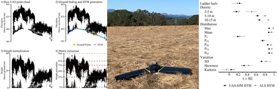
  • Determine the ability, as compared with ALS, of UAS-SfM to measure different metrics of canopy structure.
  • Demonstrate the utility of multispectral UAS-SfM in assessing the impact of wildfire on changes in photosynthetic productivity (greenness) and canopy height relative to ALS baseline conditions.
Findings from these objectives seek to answer the broad question: Can accurate measurements of forest attributes be obtained from UAS-SfM so it can be used as a stand-scale (e.g., 1 to 500 ha) remote-sensing monitoring tool to assess fire fuels and post-fire changes?

2. Materials and Methods

2.1. Study Site

This study took place at Pepperwood Preserve (38.57° N, 122.68° W), a 1261 ha nature preserve in Sonoma County, California, USA (Figure 1A). Located in the northern Coast Range, the property has predominantly rolling hills (61–475 m elevation) vegetated with a mosaic of Douglas-fir forest, oak woodland, chaparral, and grassland (Figure 1B) [29,30]. The area is characterized by a Mediterranean climate with dry, hot summers (April to October) reaching over 37 °C and mild, wet winters (November to March) infrequently dropping below 0 °C. The preserve experiences high interannual precipitation variability but receives, on average, around 86 cm of precipitation per year.
As is common throughout California, this climatic regime generates conditions for wildfires by late summer, due to sustained drying of fuels and vegetation, that are further exacerbated by strong autumnal winds [31]. In 2017, the Tubbs Fire swept through Pepperwood (Figure 1C), burning over 95% of the preserve [32]. This fire was the fourth deadliest and second most destructive in California history prior to 2020 [33,34]. The fire ignited on 9 October 2017 4:45 UTC as part of a complex of fires in the region north of San Francisco, CA. Strong easterly Diablo winds rapidly spread the fire during the first 12 h after ignition [31]. During its 23-day span, the Tubbs fire burned 14,895 ha across all vegetation types in the region.

2.2. Data Sources

2.2.1. Unoccupied Aerial System (UAS) Structure from Motion (SfM) Multispectral Data Collection and Processing

This study employed a SenseFly eBee X fixed-wing UAS platform with a MicaSense RedEdge-MX sensor onboard. This multispectral sensor collects five spectral bands: blue (475 nm center, 20 nm bandwidth), green (560 nm center, 20 nm bandwidth), red (668 nm center, 10 nm bandwidth), red edge (717 nm center, 10 nm bandwidth), and near-IR (840 nm center, 40 nm bandwidth). Additionally, an onboard MicaSense Downwelling Light Sensor (DLS) 2 collected ambient sunlight and sun angle. Due to variations in solar light intensity, sensor radiance values must be standardized to reflectance and calibrated based on a sample of known reflectance values in order for multispectral measurements to be comparable across flight missions performed on different days or under varying light conditions, as well as to be compared against reflectance data from other sensors, such as multispectral satellite images. Radiance data were converted to reflectance using downwelling radiance measured from the DLS2 and calibrated with images of a MicaSense calibration panel (RP04-1926247-OB) captured on the ground immediately before or after each flight.
We flew the UAS for 13 days between 27 September 2019 and 8 October 2019 under leaf-on conditions (i.e., leaves present on deciduous trees) and clear-sky conditions, almost exactly two years after the Tubbs fire. All flights were conducted within two hours of solar noon to minimize shadowing. We divided the study coverage area (Figure 1B,C, black boxes) into 11 flight mission zones based on battery flight-time limitations. These 11 boxes had an average size of 33 ha and total area of 332 ha. SenseFly’s eMotion 3 software (version 3.7) and a ground station controlled the UAS. The UAS flew autonomously using pre-planned missions to ensure consistent coverage and flight characteristics. Flight plans utilized eMotion’s built-in flight control function and a raster digital surface model (DSM) from the 2013 ALS mission (Section 2.2.2). This function adjusts flight altitude in order to maintain a 122-m (400-ft) flying height above the DSM. Flights were conducted with a 75% latitudinal and longitudinal image overlap. We flew each mission zone twice, employing a perpendicular “lawn mower” pattern to form a cross hatch grid. To improve georeferencing, at least three ground control points (GCPs, i.e., visible targets) were distributed throughout the mission zone prior to each flight. We obtained GPS coordinates of each GCP from >100 readings using a Trimble Juno SB and differential correction with Pathfinder Office. GCPs had a mean horizontal accuracy of 2.35 m and vertical accuracy of 2.65 m.
We processed the resulting images using Pix4Dmapper (Pix4D, Lausanne, Switzerland, version 4.4.12), which performed the reflectance calibration and generated reflectance orthomosaics for each spectral band with an 8 cm pixel size and a three-dimensional point cloud from the green spectral band. The point cloud had an average point density of 180 points/m2. The resulting point clouds had a mean RMS error from the GCPs of 1.5 m, with the exception of one highly erroneous GCP. This point was not found to affect the overall georeferencing of the resulting point cloud. We calculated pixel-level Normalized Difference Vegetation Index (NDVI) values using the red and near-IR orthomosaic images and merged the spectral data, including NDVI, with the point cloud in R (version 3.6.3) using the lidR and raster packages [35,36,37].

2.2.2. Airborne Laser Scanner (ALS) Data

We obtained ALS data from the 2013 Sonoma County Vegetation Mapping and Lidar Program website (www.sonomavegmap.org, accessed on 30 September 2019). Watershed Sciences, Inc. (Portland, OR, USA) collected these data between 28 September 2013 and 26 November 2013 using aircraft-mounted ALS50 and ALS70 sensors at a pulse density of >8 pulses/m2 [38]. The point cloud had an average point density of 15 points/m2 and an average point density in vegetation of 9.2 points/m2. The survey employed 9685 GCPs with a maximum x, y, z RMSE of 0.2 cm. Watershed Sciences conducted ground point classification using TerraSolid software and refined the point classification using a subsequent statistical surface algorithm.

2.2.3. Vegetation Distribution Data

We obtained vegetation distribution data for Pepperwood Preserve from Ackerly et al. [29]. They generated their vegetation distribution map from imagery obtained by the National Aeronautics and Space Administration’s Jet Propulsion Lab using the Airborne Visible Infrared Spectrometer-Next Generation (AVIRIS-NG) on 5 June 2014. Ackerly et al. classified this hyperspectral imagery with a support vector machine algorithm, first with broad land-cover classes, then at the tree species level in forest pixels. For the purposes of this study, we grouped tree species pixels into three generalized forest types: conifer (Pseudotsuga menziesii and Sequoia sempervirens), evergreen broadleaf (Arbutus menziesii, Notholithocarpus densiflorus, Quercus agrifolia, and Umbellularia californica), and deciduous broadleaf (Acer macrophyllum, Aesculus california, Quercus douglasii, Quercus garryana, Quercus kelloggii, and Quercus lobata).

2.2.4. 2017 Tubbs Fire Burn Severity Data

We obtained burn severity data for the 2017 Tubbs Fire from the Monitoring Trends in Burn Severity (MTBS) 2017 burn severity mosaic [39,40] (Figure 1C). This dataset utilizes the relative delta normalized burn ratio (RdNBR) [41] which analysts classify by fire into burn severity categories [39,40].

2.3. Data Analysis

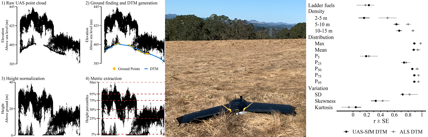
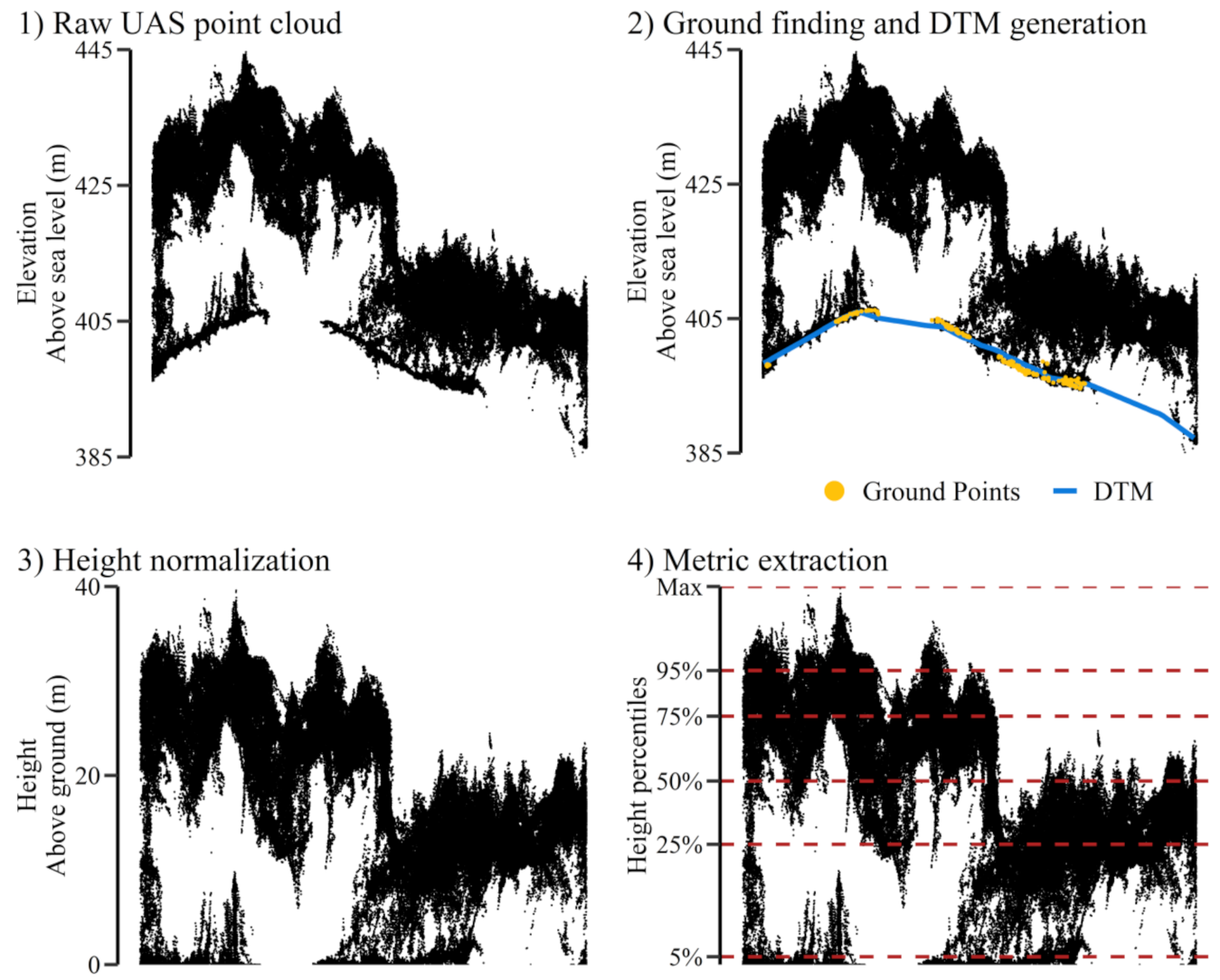
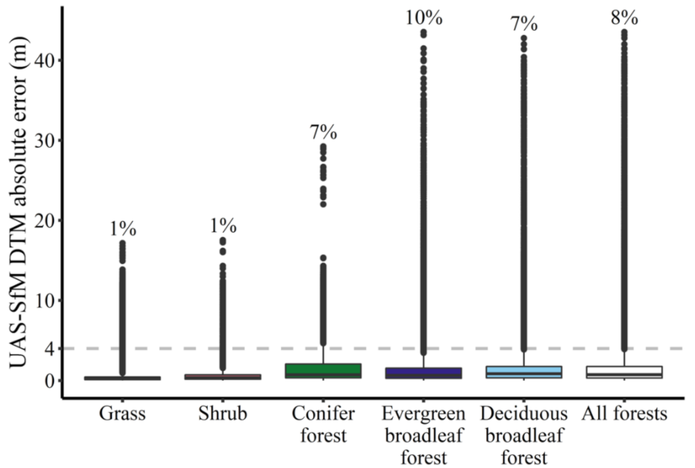
2.3.1. Digital Terrain Model (DTM) Generation Capability Analysis

DTMs are commonly generated from point cloud data by filtering for ground points and then interpolating a raster surface from these points [42]. A number of ground-filtering methods and algorithms exist and perform comparably well [43], including the cloth simulation filter (CSF) from Zhang et al. [44]. The CSF classifies ground points based on the behavior of a simulated cloth draped over an inverted version of the point cloud. Four parameters determine the performance of the cloth: rigidness, the ability of the cloth to bend; grid resolution, the spacing of cloth particles; distance threshold, the maximum distance from the cloth for a point to be classified as ground; and, time step, the movement between iterations. Rigidness only has three possible states, corresponding to the number of times a simulated cloth particle can be moved per step, while the other parameters can take any positive value. Compared to other ground-finding algorithms, the accessible parameters of the CSF algorithm render it well suited to applications in challenging forest environments where algorithm optimization must be conducted to reduce DTM generation error.
In our study site, the ground in September to October is generally covered with dirt or senesced grass, both of which have low NDVI values relative to understory vegetation. We employed the CSF in conjunction with a novel post-processing NDVI filter that takes advantage of the NDVI contrast between ground and understory components. After CSF classification of ground points, we applied a filter to reclassify all ground points with an NDVI above a threshold value. This filter removes misclassified photosynthetic understory vegetation points from the preexisting set of ground points. We generated DTMs from the identified and filtered ground points using a triangulated irregular network (TIN) to grid interpolation at one-meter resolution. Ground finding and DTM generation were conducted using the lidR package in R [38].
To optimize DTM generation for the varied forests of Pepperwood, we iterated each CSF parameter and the post-processing NDVI filter threshold over an extreme range of values while holding all other parameters constant (Table 1). Due to the relatively high accuracy of ALS DTMs, we considered any deviation of the UAS-SfM DTM from the ALS DTM to be erroneous. We produced error rasters comparing the resulting sequence of DTMs to the ALS-derived benchmark. We registered the UAS-SfM point cloud to the ALS data using the iterative closest point (ICP) algorithm in the software Lidar360 (GreenValley International, Berkeley, CA, USA, version 4.0; RMSE range: 1.57–2.34 m), and applied the resulting transformation matrices to the UAS-SfM point cloud in R. This ICP step was conducted prior to DTM error analysis using the complete UAS-SfM and ALS point clouds in order to align the ground and ensure any detected deviance in the UAS-SfM DTM produced was due to ground finding error and the DTM generation process, rather than due to a systematic offset between the point clouds. We limited this analysis to flight mission interiors at least 50 m from the mission edge to reduce the effect of edge artifacts. We calculated root mean squared error (RMSE) for the entirety of the study site as well as by vegetation type.
We conducted a second round of CSF parameter testing across the range of minimum RMSE values from the first round using a smaller step between iterations to further refine parameter values. As in round one, each parameter was run through its range while the other parameters were held constant. As mentioned previously, rigidness only has three distinct levels. Therefore, we did not repeat the iteration process for rigidness in round two. Unlike the first round, we conducted this second round in a stepwise manner, whereby the constant value for a parameter was updated to its newly identified optimum before proceeding with the next parameter assessment. A parameter’s relative effect on RMSE in round one determined the order of optimization for this second round. We optimized grid resolution first, holding the other parameters at the constant corresponding to the minimum RMSE obtained in round one. Time step was optimized second, using the updated round two optimized grid resolution value, along with the other constants from round one. Distance threshold was parameterized third and NDVI threshold last, again updating parameters to their new values before proceeding. Final optimized CSF parameter values corresponded to the minimum RMSE obtained in round two. We produced a final UAS-SfM DTM from this set of optimized parameters using TIN-to-grid interpolation. We then calculated absolute error (relative to the ALS DTM) for each raster cell and separated this error by vegetation type.

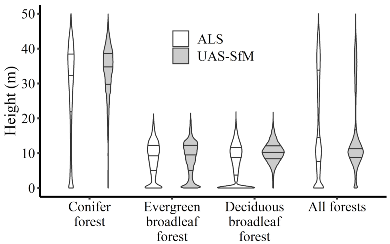
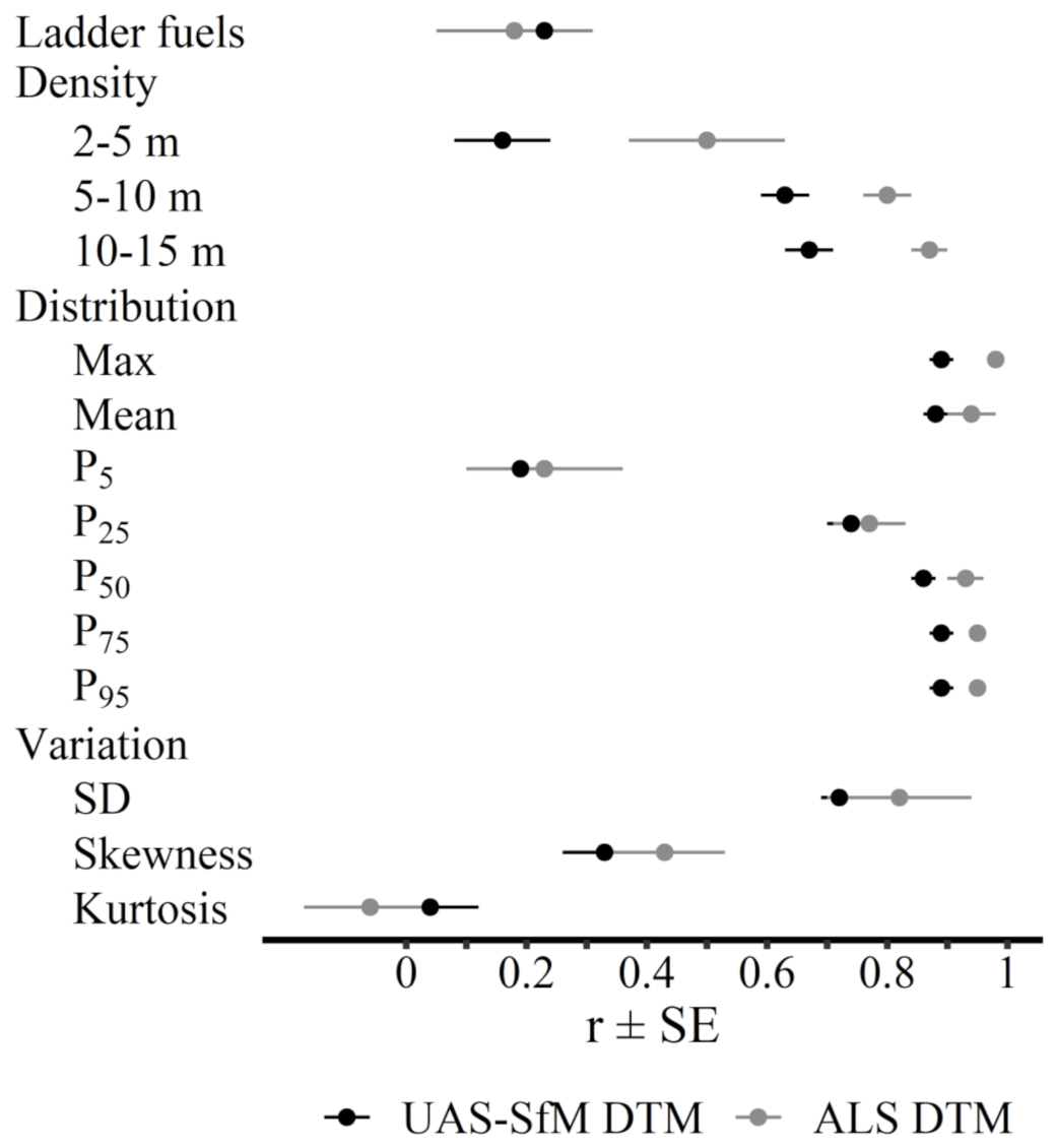
2.3.2. Comparison of Forest Structure from UAS-SfM and ALS Point Clouds

We first compared the actual vertical height point cloud structures of UAS-SfM and ALS height-normalized point cloud data for each forest type. We then compared vertical height structure metrics between these data types. The general workflow for extracting vegetation structure metrics from point cloud data involves: (1) height normalizing the data against a digital terrain model (DTM) to isolate canopy height from terrain features, and (2) extracting metrics from these normalized data (Figure 2). We conducted this height normalization process on the original, unregistered UAS-SfM point cloud in two ways. First, to determine the capability of UAS-SfM as a standalone method for measuring forest structure, we height normalized the UAS-SfM point cloud using the UAS-SfM DTM produced through the previously described CSF optimization (Section 2.3.1). Second, to determine the enhanced capability of UAS-SfM in areas with preexisting high-resolution DTMs, we height normalized the UAS-SfM point cloud using the ALS DTM. To correct for any systematic vertical and horizontal location bias separating the UAS-SfM point cloud and the ALS DTM, we registered the UAS-SfM ground points to the ALS DTM prior to height normalization. We generated transformation matrices for the alignment of the UAS-SfM ground points to the ALS DTM using the ICP algorithm in Lidar360, and applied the matrices to the entire UAS-SfM point cloud in R. This method allowed for registration based solely on the ground points to avoid overfitting of canopy metric comparisons as would occur if the entire point clouds had been used for registration purposes.
Using these height normalized data, we compared area-based height metrics between both UAS-SfM datasets and ALS. A subset of metrics from Filippelli et al. [8] were computed at a 20 × 20-m grid scale. While the high resolution of UAS-SfM data permits analysis at finer spatial scales, this larger grid scale was selected to align with a preexisting plot network at Pepperwood. Additionally, the MTBS burn severity dataset is assessed at 30 m resolution, limiting finer scale analysis of differences between burn severities. Density metrics represented the percentage of 3D points within a grid cell that fell within a particular vertical height band. Other metrics from each cell included height percentiles (P5, P25, P50, P75, and P95), mean, maximum, standard deviation, skewness, and kurtosis of point cloud heights. To reduce confounding factors of mixed species and structural change due to fire, respectively, we filtered grid cells for only those cells covered by at least 75% of one forest type and with a burn severity of unchanged or low. From this filtered dataset, we computed the slope linear regression coefficient and Pearson’s correlation coefficient for the relationship between UAS-SfM and ALS values for each of these metrics. This was done using 10,000 bootstrap replicates of 100 grid cells per forest type to correct for spatial autocorrelation and maintain balanced sample sizes. In addition to these standard metrics of point cloud height, we compared the ladder fuel metric from Green et al. [45] between the two datasets in the same way as the other metrics. This metric is calculated as the number of points between 1 and 4 m divided by the total number of points below 4 m and was shown to significantly contribute to canopy damage in local non-wind-driven fires, including the Tubbs Fire.

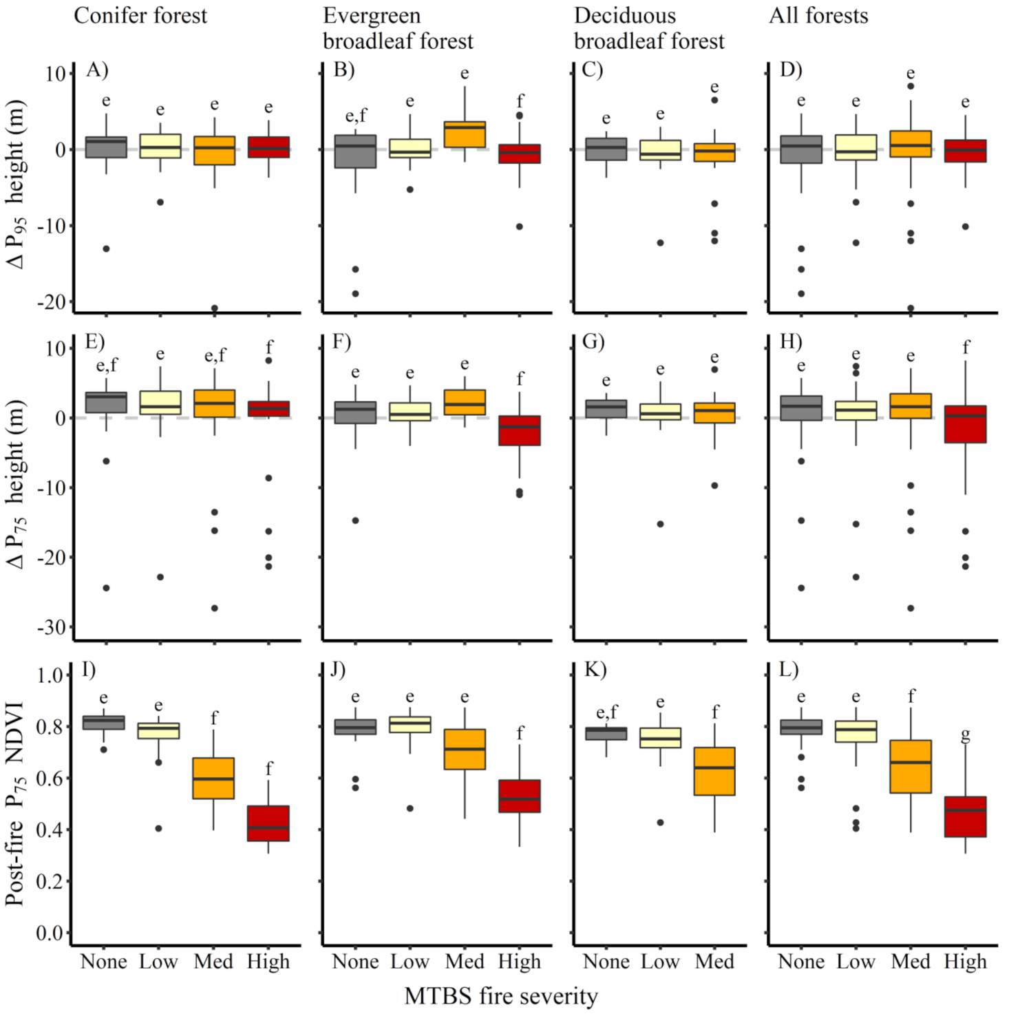
2.3.3. Utility of UAS-SfM for Detecting Post-Fire Forest Change

We took a random sample of 20 grid cells per forest type (conifer, broadleaf evergreen, broadleaf deciduous) from each of the four burn severity classes (none, low, medium, and high). High burn severity data in deciduous broadleaf forest was excluded from all Tubbs Fire analysis due to insufficient sample size (n = 8 grid cells). These data were found to violate normality, so non-parametric statistical tests were implemented in subsequent analyses.
We determined the influence of ladder fuels on Tubbs Fire burn severity by forest type. Ladder fuels from the ALS data were used in this analysis since these data represented pre-fire conditions (four-year difference). We conducted a Kruskal–Wallis one-way analysis of variance to test differences in mean rank ladder fuel density among burn severity classes for the three forest types. Significant results were followed by Dunn’s post-hoc test to examine the nature of between-group differences. We adjusted p-values via the Bonferroni method to account for multiple comparisons.
We determined the impact of fire severity in the Tubbs Fire on forest canopy structure using the 95th percentile height (P95) metric and 75th percentile height (P75) metrics. Since these metrics are highly positively correlated between UAS-SfM and ALS data with regression coefficients close to one (Table 2), the two can be directly compared for assessing change in canopy structure [8]. In this case, ALS represents pre-fire canopy conditions and UAS-SfM represents post-fire conditions. We also tested differences in mean rank of P95 and P75 canopy metrics, respectively, among burn severity classes by forest type using a Kruskal–Wallis one-way analysis of variance test. Significant results were followed by Dunn’s post-hoc tests to examine the nature of between-group differences. We adjusted p-values via the Bonferroni method to account for multiple comparisons. For this analysis, we used the UAS-SfM dataset height normalized using the ALS DTM.
Lastly, we used mean NDVI at the P75 canopy height to determine the impact of fire severity on canopy health. In the absence of pre-fire NDVI values, we used the unburned forest stands as the control reference for the purpose of detecting the fire’s impact. As before, we tested the differences in mean rank P75 canopy metrics among burn severity classes by forest type using a Kruskal–Wallis test with a Dunn’s post-hoc test for between-group differences and Bonferroni adjusted p-values.

3. Results

3.1. DTM and CHM Generation Capability Comparisons

Compared to the baseline ALS DTM, two rounds of CSF parameter optimization achieved a UAS-SfM-derived DTM with a minimum RMSE of 2.12 m across the study site (Figure 3I). This was a reduction of 1.68 m of error relative to the DTM generated from CSF default parameters (Figure 3A). Responses to parameter changes were largely consistent among vegetation types. Therefore, parameter optimization could be conducted across the full study site without sacrificing accuracy in any given vegetation type. Across the wide range of the first round of parameter testing, the rigidness and distance threshold parameters had minimal effect (Figure 3C,D), while the grid resolution and time step parameters greatly affected both DTM accuracy and processing time (Figure 3A,B). In particular, grid resolution processing times rose sharply as the resolution approached zero.
The post-processing NDVI threshold filter reduced UAS-SfM DTM error in both rounds of processing (Figure 3E,I). Compared to the DTM produced from the CSF default parameters alone, the NDVI filter reduced site-wide RMSE by 0.73 m, down to 3.07 m (Figure 3E). In comparison, two rounds of parameter optimization without the NDVI filter reduced site-wide RMSE by only 0.66 m. The performance of the NDVI filter was even more pronounced in the second round. With optimal values for other CSF parameters in place, the addition of the NDVI filter reduced site-wide RMSE by 1.02 m (Figure 3I). Therefore, of the final achieved optimization improvement of 1.68 m, ~61% was due to the NDVI threshold filter. Additional processing time for this filter was negligible. When the error analysis was limited from the entire DTM to just the identified ground points, regression results between these ground points and the corresponding elevation of the ALS DTM show a strong positive relationship (r ≈ +1, slope ≈ +1). This confirms the CSF process accurately identifies ground points.
However, the distribution of absolute error from all 1 m cells of the UAS-SfM DTM, when compared to an ALS DTM, showed a substantial number of extreme outliers across all vegetation types, and, in some cases, higher than the canopy height (Figure 4). While the ground finding process improved overall DTM accuracy, the measurement limitations of UAS-SfM meant that it was unable to detect any ground points in some regions with substantial changes in terrain height, subsequently resulting in DTM errors observed in those areas. Based on their respective interquartile ranges, UAS-SfM DTM generation appears to demonstrate greater consistency in accuracy for grasslands than forested areas. However, due to the number of outliers across vegetation types, statistical analyses could not be conducted to differentiate DTM accuracy by vegetation type. Errors over 15 m were observed even in a few grasslands, indicating that large errors can appear even in areas without canopy cover. Errors over 4 m represent locations where the DTM inaccuracy would be so great as to render detection of ladder fuels largely impossible. Eight percent of the combined forest UAS-SfM DTM cells had errors greater than 4 m, while only 1% of grass and shrub cells had errors above this threshold, respectively. When separated by forest type, the forest cell error percentages ranged from 7–10%.

3.2. Comparison of Forest Structure from UAS-SfM and ALS Point Clouds

The vertical structure of UAS-SfM and ALS point clouds reflect the ability of each sensor to detect structure below the canopy. Across all forest types for the complete site-wide dataset, ALS point clouds had a negatively tapered vertical density from the middle to lower part of forest canopies and a high density of ground points (Figure 5). The UAS-SfM point cloud upper-canopy density structure closely resembled that of ALS data, reaching a maximum canopy point density at a similar height. However, the lower canopy structure for UAS data tapered rapidly, indicating that the UAS point cloud was generally unable to detect the ground under heavy tree canopy. However, an exception to this pattern was observed in the evergreen broadleaf forest, which exhibited an increased point density at ground level. The unburned stand of evergreen broadleaf forest in this analysis contained trees spatially separated from one another, and it is from these gaps between the trees that the ground points were measured. Therefore, the increase in ground points does not actually represent an increased ability of UAS-SfM to detect below canopy structure in this forest type.
The area-based metric comparisons between UAS-SfM and ALS data reflect the preceding observations on sub-canopy detection across vegetation types (Table 2 and Table 3). For both the UAS-SfM height metrics extracted using the UAS-SfM derived DTM and the ALS DTM for height normalization, only metrics associated with the upper half of the canopy (e.g., P50, P75, P95, mean height, and max height) exhibited Pearson’s r > +0.80. No relationships of this type exist between UAS-SfM and ALS for any of the metrics of height variation, nor those of height density for either of the height normalization approaches, with the exception of upper-canopy density (10–15 m) from the ALS DTM normalized dataset. As expected from the errors identified during the UAS-SfM DTM generation analysis (Section 3.1), the metrics extracted from the UAS-SfM data height normalized using the ALS DTM systematically performed better than the UAS-SfM data height normalized using the UAS-SfM DTM. However, these differences were small, especially for percentile metrics associated with the upper half of the canopy (Figure 6).

3.3. Utility of UAS-SfM for Detecting Post-Fire Forest Change

Ladder fuels: Across all forest types, the mean rank ladder fuel density was significantly higher in the high burn severity class, as compared to all other areas (Table 4, Figure 7). In evergreen broadleaf forests, the mean rank ladder fuel density was significantly lower in the medium burn severity class, as compared to the unburned and high burn severities classes (Table 4, Figure 7). The ladder fuel densities did not differ among burn severities for the other forest types.
∆P95: In evergreen broadleaf forests, the mean rank in pre-fire (ALS) to post-fire (UAS-SfM) P95 canopy height change (∆P95) was significantly more negative (i.e., greater decrease in heights) in the high burn severity class as compared to the low and medium burn severity classes (Table 4, Figure 8B). The mean rank ∆P95 was not significantly different across burn severities in the other forest types or for all forests combined (Table 4, Figure 8B–D).
∆P75: Across all forest types and in evergreen broadleaf forests, the mean rank ∆P75 was significantly more negative in the high burn severity class as compared to all others (Table 4, Figure 8F,H). In conifer forests, the mean rank ∆P75 was significantly more negative in the high burn severity class as compared to the low burn severity (Table 4, Figure 8E). The mean rank ∆P75 did not differ in deciduous broadleaf forests.
P75NDVI: Across all forest types and in evergreen broadleaf forests, the mean rank in NDVI at post-fire (UAS) P75 canopy height (P75 NDVI) was significantly lower in the high burn severity class as compared to all others (Table 4, Figure 8L,J). In addition, across all forest types, the mean rank P75 was significantly lower in the medium burn severity class as compared to the low and unburned classes (Table 4, Figure 8L). In conifer forests, the mean rank in P75 NDVI was significantly lower in the medium and high burn severity classes as compared to all others (Table 4, Figure 8I). In deciduous broadleaf forests, the mean rank in P75 NDVI was significantly lower in the medium burn severity class as compared to the low burn severity class (Table 4, Figure 8K).
In summary, only evergreen broadleaf forests exhibited a change in 95th percentile canopy height at higher burn severities. Bulk canopy height, represented by the 75th height percentile, decreased at high burn severity when considering all forests together, and within evergreen broadleaf and conifer forests. We also found that NDVI values in the bulk canopy decreased (i.e., lower greenness) with increasing burn severity, regardless of forest type.

4. Discussion

4.1. DTM and CHM Generation Capability Comparisons

This study sought to assess the capacity of UAS-SfM as a stand-alone forest monitoring tool to be employed in Mediterranean forests without pre-existing ALS data. This requires that a sufficiently accurate DTM can be estimated from UAS-SfM 3D point clouds, considering both detection of ground points and the classification of these points as ground relative to understory vegetation. This terrain finding process enables the isolation of canopy-height from topography. While it is possible to achieve sub-centimeter DTM accuracy from UAS-SfM for bare ground conditions [46], increasing vegetation cover heavily impacts DTM accuracy [47,48,49]. Through two rounds of ground finding parameter optimization, we achieved a site wide DTM RMSE of 2.12 m. However, 8% of DTM coverage in forest areas contained errors over 4 m. This height threshold represents the upper limit of the ladder fuel metric from Green et al. [45], so errors of this magnitude connote an inability to detect surface or ladder fuels.
While the proliferation of error of this magnitude is serious, deciding whether this represents an unacceptable level of error largely depends on the context in which these data will be used. To determine canopy height and other metrics in areas of dense forest, having a baseline DTM from a more reliable source, such as airborne or UAS lidar, will always be best practice [50,51], assuming terrain does not change considerably over a study time period. However, in situations where these data do not exist, 8% error coverage may have to represent an acceptable margin. Of perhaps more importance among this erroneous area are the individual DTM sites with extreme errors, linked with gaps in the distribution of detected ground points. Future research should analyze the role of topography and canopy type in producing these areas of extreme error magnitude in order to determine conditions under which UAS-SfM cannot function without a preexisting DTM. Another future avenue of research to avoid these errors entirely is to determine if DTM-independent methods for extraction of forest metrics, which have been validated in forestry growing stock volume measurements [52], can be applied to the mapping of fuel loads.
This study employed the Cloth Simulation Filter (CSF) from Zhang et al. [44] in conjunction with a subsequent NDVI filter to classify ground points from which a DTM could be generated through interpolation. In Mediterranean shrublands, Carvajal-Ramirez et al. [53] found the CSF performance was weaker relative to an NDVI classifier, and the authors called for the need to assess the impact of CSF parameter setting on ground-finding accuracy. In this study, CSF parameter optimization alone only marginally improved RMSE over the default parameters. However, the addition of our NDVI threshold filter resulted in a large (>60%) improvement in RMSE. Drawing on the concept of the NDVI classifier from Carvajal-Ramirez et al. [53], the combination of CSF with an NDVI filter leverages the strengths of both methods. The CSF identifies an initial set of ground points from which the NDVI filter removes misclassified vegetation. When multispectral data exist, this filter provides a computationally simple way to improve ground finding based on point cloud structure alone. While methods for ground finding are continually being developed or improved e.g., [54], this filter provides an additional tool in mitigating the subcanopy detection shortcomings of UAS-SfM. However, one important caveat to our results is that our study area benefits from relatively low senesced grass (depending on cattle rotations and deer grazing) and higher live shrubs in late summer, thereby providing a strong NDVI contrast that aids the ground filter. Further tests of the CSF and NDVI filter combination in other ecosystems are certainly warranted.

4.2. Comparison of Forest Structure from UAS-SfM and ALS Point Clouds

Linear regression comparisons between UAS-SfM and ALS confirm past findings from other forest types and applications that UAS-SfM can only reliably resolve upper-canopy structure, but does so with a high degree of accuracy e.g., [49,55]. The analysis presented here closely matches Filippelli et al. [8], who found similar relationships in a montane coniferous and lodgepole pine forest between ALS and SfM DAP collected using an airplane flown at high altitude and with lower image overlap than used in this study. This suggests that SfM DAP has the same strength and limitations irrespective of image acquisition method and forest type. In particular, SfM DAP provides a powerful tool for measuring upper-canopy forest structure. The strength of this tool is dependent on the accuracy of the DTM underlying the analysis. While the use of the ALS DTM for height normalization systematically improved the accuracy of extracted canopy metrics as compared to the UAS-SfM, both methods performed well in measuring all metrics associated with the upper half of the canopy.
For SfM DAP to determine a point’s 3D location, it must appear in multiple overlapping images. Therefore, the technique often fails to detect gaps in canopy cover, let alone resolve what lies below the canopy [28]. In our study, this shortcoming was most acutely demonstrated in our attempt to measure ladder fuels. No relationship existed between the ALS and UAS-SfM derived metrics. SfM DAP overestimates metrics of density, such as the ladder fuels metric, and canopy cover due to this lack of subcanopy detection [50]. The analysis of the point cloud’s respective vertical structure lends additional weight to the conclusion that UAS-SfM cannot measure ladder fuels using the same metric as is employed for ALS. However, this study was limited in this analysis due to the six years between the collection of ALS and UAS-SfM data. While we restricted this analysis to areas of the study site unaffected by the Tubbs Fire, forest structure may have changed during the interim period (e.g., tree growth, disease, or mortality), which may account for some of the measured UAS-SfM error relative to the ALS baseline. Despite the subcanopy detection limitations of SfM DAP, Filippelli et al. [8] found DAP models of canopy structure performed comparably to those derived from ALS. Future studies with coincident ALS and UAS-SfM data should investigate this relationship further to determine if other methods can measure ladder fuel density from UAS-SfM despite its limitations under high canopy cover.

4.3. Utility of UAS-SfM for Detecting Post-Fire Forest Change

Two years after the Tubbs Fire swept through Pepperwood, UAS-SfM found minimal changes in canopy height relative to pre-fire metrics. In the aggregate analysis of all forest types, measures of maximum height (95th percentile) did not change, while bulk canopy height (75th percentile) decreased significantly in regions with the highest burn severity. We observed significant decreases in NDVI with increasing burn severity across all forests regardless of structural change. While we did not have calibrated pre-fire measures of NDVI on the same spatial scale to which we could compare, the unburned areas were used as a control reference in this comparison. This demonstrates the long-lasting impact a severe wildfire has on Mediterranean forest health.
The role of NDVI in understanding forest health indicates that multispectral sensors have an important role in forest monitoring for fire hazard and post-fire recovery. Change in NDVI can detect fine-scale forest physiological stress [56]. Change in NDVI also provides the best estimator of post-fire severity in Mediterranean vegetation [45,57]. The long-term trend of NDVI over a stand or ecosystem can be used to measure the degree to which different vegetation types manage to recover from a severe fire event [58]. In our study ecosystem, UAS-SfM-based measures of NDVI or other greenness indices over multiple times post-fire could provide valuable crown-scale information on tree response to fire [59,60], such as initiation of epicormic sprouting and subsequent canopy growth. As demonstrated here, this information can provide insight on impacts beyond what structural information alone could provide. In addition, since multispectral UAS-SfM provides coupled spectral and structural information, it offers a means to target analysis at particular levels of the canopy in a way that is not possible with aerial or satellite imagery alone. For example, here we were able to use this technology to disentangle bulk canopy changes in NDVI from other post-fire ecosystem changes, such as ground vegetation recovery. While our results targeted change detection at the 20 m grid level, future studies should leverage the high resolution of this technology to analyze change at finer scales or even at the individual tree level.
The analysis of post-fire canopy changes would not have been possible without the existence of the pre-fire ALS data. While the unburned areas could be used as a control in the absence of such data, as done here with the NDVI analysis, change analysis of this type greatly benefits from ongoing monitoring. It is in this capacity that UAS-SfM provides a particularly strong benefit due to the ease of data acquisition at plot to stand scales.
Although UAS-SfM could not estimate ladder fuels, our analysis with ALS-based pre-fire ladder fuels and burn severity revealed a pattern that merits further investigation. In the aggregate analysis of all forest types, the high burn severity class exhibited greater pre-fire ladder fuel density than the low burn severity class. We found a significant relationship between increasing pre-fire ladder fuel densities and medium to high burn severity in evergreen broadleaf forest, but not in the conifer forest. Neither forest type had a significant difference between low and high burn severities. Conifers in particular showed no relationship between burn severity and ladder fuel density. Two explanations are possible for this. First, the majority of conifer forest that burned at high severity during the Tubbs Fire did so during the initial “Diablo” wind-driven portion of the event. Green et al. [45] identified these winds to be an even stronger driver of burn severity than ladder fuels. Therefore, the mixed signal across forest types and in conifer forests may be attributable to wind strength overwhelming any difference that ladder fuel densities may have otherwise caused in burn severity [61]. An alternative explanation, however, is that the ladder fuel metric employed here performs well in shorter evergreen broadleaf forests, especially in determining if higher intensities fires are able to cross the high severity threshold, but does not apply in tall conifer forests where canopy base height may be well above 4 m. Further work is needed to investigate the utility of different measures of vertical fuel continuity, such as ladder fuel metrics, in different forest types. Furthermore, the estimation of such sub-canopy metrics at a stand scale using UAS may best be achieved with an attached lidar sensor instead of the SfM approach used here [62]. Although UAS-SfM is currently more economical, prices for UAS lidar are expected to decrease over time [25].

5. Conclusions

For fire hazard mitigation land management treatments to be effective, land managers must implement them at broad spatial scales, from single forest stands to larger regions [63]. This requires an improved understanding of forest structure and fuel loading to inform management practices.
Due to the comparatively low investment in time or resources involved in conducting repeated data collection missions, UAS-SfM provides a unique opportunity to monitor ongoing changes and recovery of forest structure and physiological health following major disturbance events at plot to stand scales [26,64]. Our study in a Mediterranean forest site in Northern California found UAS-SfM able to accurately detect ground points. However, ground points in some areas were too sparsely distributed to reliably estimate ground elevation, a limitation that affects subsequent canopy height retrieval and limits its use in these areas as a stand-alone tool in the absence of more accurate terrain data. This shortcoming arose from UAS-SfM’s limited subcanopy detection ability, which also hindered its ability to detect ladder fuels and other below-canopy metrics. Across the study site, UAS-SfM excelled at mapping the upper canopy of forests and, when combined with a multispectral sensor, can provide information on vegetation productivity and physiological stress. This accuracy can be improved further when the UAS-SfM is paired with an accurate baseline measurement of ground elevation (e.g., from an airborne lidar sensor). UAS-SfM, therefore, provides a valuable tool for monitoring post-fire impacts and recovery through the use of upper-canopy metrics of structure and health, especially at sites with pre-fire data as presented here. Much work remains to be done in the evaluation of UAS-SfM as a fire fuel monitoring tool in Mediterranean ecosystems. Future work should focus on leveraging the strengths of this method to improve management outcomes.

Author Contributions

Conceptualization, S.R., M.L.C., L.P.B. and I.O.M.; methodology, S.R., M.L.C., L.P.B. and I.O.M.; investigation, S.R., M.L.C., L.P.B., C.M. and E.P.; software, S.R. and M.L.C.; formal analysis, S.R. and M.L.C.; resources, M.L.C. and L.P.B.; writing—original draft preparation, S.R.; writing—review and editing, I.O.M., M.L.C., L.P.B., C.M. and E.P.; visualization, S.R.; supervision, I.O.M., M.L.C. and L.P.B.; funding acquisition, L.P.B. and M.L.C. All authors have read and agreed to the published version of the manuscript.

Funding

Funding for this research was supported by CAL FIRE Forest Health and Forest Legacy (8GG18806) and California State University, Agricultural Research Institute (20-01-106) awards. SR was funded by the Rhodes Trust and through the University of Oxford Environmental Change Institute Small Grant Scheme.

Institutional Review Board Statement

Not applicable.

Informed Consent Statement

Not applicable.

Data Availability Statement

ALS data used in this study are available through the Sonoma Veg Map online portal (sonomavegmap.org). MTBS burn severity data used in this study are available through the MTBS online portal (mtbs.gov). UAS data are available upon request.

Acknowledgments

We thank the staff of Pepperwood Preserve for allowing us access to their beautiful site. This work is a product of the 3D Forests research group.

Conflicts of Interest

The authors declare no conflict of interest.

References

  1. Rundel, P.W.; Arroyo, M.T.K.; Cowling, R.M.; Keeley, J.E.; Lamont, B.B.; Vargas, P. Mediterranean Biomes: Evolution of Their Vegetation, Floras, and Climate. Annu. Rev. Ecol. Evol. Syst. 2016, 47, 383–407. [Google Scholar] [CrossRef]
  2. Beaty, R.M.; Taylor, A.H. Fire History and the Structure and Dynamics of a Mixed Conifer Forest Landscape in the Northern Sierra Nevada, Lake Tahoe Basin, California, USA. For. Ecol. Manag. 2008, 255, 707–719. [Google Scholar] [CrossRef]
  3. Cowling, R.; Rundel, P.; Lamont, B.; Arroyo, M.; Arianoutsou, M. Plant Diversity in Mediterranean-Climate Regions. Trends Ecol. Evol. 1996, 11, 362–366. [Google Scholar] [CrossRef]
  4. Odion, D.C.; Moritz, M.A.; DellaSala, D.A. Alternative Community States Maintained by Fire in the Klamath Mountains, USA: Fire and Alternative Community States. J. Ecol. 2010, 98, 96–105. [Google Scholar] [CrossRef]
  5. Westerling, A. Wildfire Simulations for California’s Fourth Climate Change Assessment: Projecting Changes in Extreme Wildfire Events with a Warming Climate; California’s Fourth Climate Change Assessment; California Energy Commission: Sacramento, CA, USA, 2018; p. 57.
  6. Miller, J.D.; Safford, H.D.; Crimmins, M.; Thode, A.E. Quantitative Evidence for Increasing Forest Fire Severity in the Sierra Nevada and Southern Cascade Mountains, California and Nevada, USA. Ecosystems 2009, 12, 16–32. [Google Scholar] [CrossRef]
  7. Dennison, P.E.; Brewer, S.C.; Arnold, J.D.; Moritz, M.A. Large Wildfire Trends in the Western United States, 1984-2011. Geophys. Res. Lett. 2014, 41, 2928–2933. [Google Scholar] [CrossRef]
  8. Filippelli, S.K.; Lefsky, M.A.; Rocca, M.E. Comparison and Integration of Lidar and Photogrammetric Point Clouds for Mapping Pre-Fire Forest Structure. Remote Sens. Environ. 2019, 224, 154–166. [Google Scholar] [CrossRef]
  9. Flannigan, M.D.; Krawchuk, M.A.; de Groot, W.J.; Wotton, B.M.; Gowman, L.M. Implications of Changing Climate for Global Wildland Fire. Int. J. Wildland Fire 2009, 18, 483–507. [Google Scholar] [CrossRef]
  10. Westerling, A.L.; Bryant, B.P. Climate Change and Wildfire in California. Clim. Chang. 2008, 87, 231–249. [Google Scholar] [CrossRef]
  11. Alonzo, M.; Andersen, H.-E.; Morton, D.; Cook, B. Quantifying Boreal Forest Structure and Composition Using UAV Structure from Motion. Forests 2018, 9, 119. [Google Scholar] [CrossRef] [Green Version]
  12. Berra, E.F.; Gaulton, R.; Barr, S. Assessing Spring Phenology of a Temperate Woodland: A Multiscale Comparison of Ground, Unmanned Aerial Vehicle and Landsat Satellite Observations. Remote Sens. Environ. 2019, 223, 229–242. [Google Scholar] [CrossRef]
  13. Arroyo, L.A.; Pascual, C.; Manzanera, J.A. Fire Models and Methods to Map Fuel Types: The Role of Remote Sensing. For. Ecol. Manag. 2008, 256, 1239–1252. [Google Scholar] [CrossRef] [Green Version]
  14. Stefanidou, A.; Gitas, I.Z.; Katagis, T. A National Fuel Type Mapping Method Improvement Using Sentinel-2 Satellite Data. Geocarto Int. 2020, 1–21. [Google Scholar] [CrossRef]
  15. Andersen, H.-E.; McGaughey, R.J.; Reutebuch, S.E. Estimating Forest Canopy Fuel Parameters Using LIDAR Data. Remote Sens. Environ. 2005, 94, 441–449. [Google Scholar] [CrossRef]
  16. Marino, E.; Montes, F.; Tomé, J.L.; Navarro, J.A.; Hernando, C. Vertical Forest Structure Analysis for Wildfire Prevention: Comparing Airborne Laser Scanning Data and Stereoscopic Hemispherical Images. Int. J. Appl. Earth Obs. Geoinf. 2018, 73, 438–449. [Google Scholar] [CrossRef]
  17. Kramer, H.A.; Collins, B.M.; Kelly, M.; Stephens, S.L. Quantifying Ladder Fuels: A New Approach Using LiDAR. Forests 2014, 5, 1432–1453. [Google Scholar] [CrossRef]
  18. Menning, K.M.; Stephens, S.L. Fire Climbing in the Forest: A Semiqualitative, Semiquantitative Approach to Assessing Ladder Fuel Hazards. West. J. Appl. For. 2007, 22, 88–93. [Google Scholar] [CrossRef] [Green Version]
  19. Donnellan, A.; Harding, D.; Lundgren, P.; Wessels, K.; Gardner, A.; Simard, M.; Parrish, C.; Jones, C.; Lou, Y.; Stoker, J.; et al. Observing Earth’s Changing Surface Topography and Vegetation Structure: A Framework for the Decade; NASA Surface Topography and Vegetation Incubation Study; NASA: Washington, DC, USA, 2021; p. 210.
  20. Chuvieco, E.; Aguado, I.; Salas, J.; García, M.; Yebra, M.; Oliva, P. Satellite Remote Sensing Contributions to Wildland Fire Science and Management. Curr. For. Rep. 2020, 6, 81–96. [Google Scholar] [CrossRef]
  21. Dandois, J.P.; Olano, M.; Ellis, E.C. Optimal Altitude, Overlap, and Weather Conditions for Computer Vision UAV Estimates of Forest Structure. Remote Sens. 2015, 7, 13895–13920. [Google Scholar] [CrossRef] [Green Version]
  22. Alonzo, M.; Dial, R.J.; Schulz, B.K.; Andersen, H.-E.; Lewis-Clark, E.; Cook, B.D.; Morton, D.C. Mapping Tall Shrub Biomass in Alaska at Landscape Scale Using Structure-from-Motion Photogrammetry and Lidar. Remote Sens. Environ. 2020, 245, 111841. [Google Scholar] [CrossRef]
  23. Dandois, J.P.; Ellis, E.C. High Spatial Resolution Three-Dimensional Mapping of Vegetation Spectral Dynamics Using Computer Vision. Remote Sens. Environ. 2013, 136, 259–276. [Google Scholar] [CrossRef] [Green Version]
  24. Tompalski, P.; White, J.C.; Coops, N.C.; Wulder, M.A. Quantifying the Contribution of Spectral Metrics Derived from Digital Aerial Photogrammetry to Area-Based Models of Forest Inventory Attributes. Remote Sens. Environ. 2019, 234, 111434. [Google Scholar] [CrossRef]
  25. Hu, T.; Sun, X.; Su, Y.; Guan, H.; Sun, Q.; Kelly, M.; Guo, Q. Development and Performance Evaluation of a Very Low-Cost UAV-Lidar System for Forestry Applications. Remote Sens. 2020, 13, 77. [Google Scholar] [CrossRef]
  26. Campbell, M.J.; Dennison, P.E.; Tune, J.W.; Kannenberg, S.A.; Kerr, K.L.; Codding, B.F.; Anderegg, W.R.L. A Multi-Sensor, Multi-Scale Approach to Mapping Tree Mortality in Woodland Ecosystems. Remote Sens. Environ. 2020, 245, 111853. [Google Scholar] [CrossRef]
  27. Cunliffe, A.M.; Brazier, R.E.; Anderson, K. Ultra-Fine Grain Landscape-Scale Quantification of Dryland Vegetation Structure with Drone-Acquired Structure-from-Motion Photogrammetry. Remote Sens. Environ. 2016, 183, 129–143. [Google Scholar] [CrossRef] [Green Version]
  28. White, J.C.; Tompalski, P.; Coops, N.C.; Wulder, M.A. Comparison of Airborne Laser Scanning and Digital Stereo Imagery for Characterizing Forest Canopy Gaps in Coastal Temperate Rainforests. Remote Sens. Environ. 2018, 208, 1–14. [Google Scholar] [CrossRef]
  29. Ackerly, D.D.; Kling, M.M.; Clark, M.L.; Papper, P.; Oldfather, M.F.; Flint, A.L.; Flint, L.E. Topoclimates, Refugia, and Biotic Responses to Climate Change. Front. Ecol. Environ. 2020, 18, 288–297. [Google Scholar] [CrossRef]
  30. Evett, R.R.; Dawson, A.; Bartolome, J.W. Estimating Vegetation Reference Conditions by Combining Historical Source Analysis and Soil Phytolith Analysis at Pepperwood Preserve, Northern California Coast Ranges, U.S.A: Estimating Vegetation Reference Conditions. Restor. Ecol. 2013, 21, 464–473. [Google Scholar] [CrossRef]
  31. Nauslar, N.; Abatzoglou, J.; Marsh, P. The 2017 North Bay and Southern California Fires: A Case Study. Fire 2018, 1, 18. [Google Scholar] [CrossRef] [Green Version]
  32. Pepperwood Preserve. What Does Resilience Look like after Two Fires in Two Years? In Pepperwood Field Notes; Pepperwood Preserve: Santa Rosa, CA, USA, 2019. [Google Scholar]
  33. CalFire. Top 20 Deadliest California Wildfires; CalFire: Sacramento, CA, USA, 2019.
  34. CalFire. Top 20 Most Destructive California Wildfires; CalFire: Sacramento, CA, USA, 2019.
  35. Roussel, J.-R.; Auty, D.; De Boissieu, F.; Sánchez Meador, A.; Jean-François, B. LidR: Airborne LiDAR Data Manipulation and Visualization for Forestry Applications; R Foundation for Statistical Computing: Vienna, Austria, 2020. [Google Scholar]
  36. R Core Team. R: A Language and Environment for Statistical Computing; R Foundation for Statistical Computing: Vienna, Austria, 2019. [Google Scholar]
  37. Hijmans, R.J.; van Etten, J.; Sumner, M.; Cheng, J.; Bevan, A.; Bivand, R.; Busetto, L.; Canty, M.; Forrest, D.; Ghosh, A.; et al. Raster: Geographic Data Analysis and Modeling, R Foundation for Statistical Computing: Vienna, Austria, 2019.
  38. Watershed Sciences. Sonoma County Vegetation Mapping and Lidar Program: Technical Data Report; Watershed Sciences: Portland, OR, USA, 2016. [Google Scholar]
  39. Eidenshink, J.; Schwind, B.; Brewer, K.; Zhu, Z.-L.; Quayle, B.; Howard, S. A Project for Monitoring Trends in Burn Severity. Fire Ecol. 2007, 3, 3–21. [Google Scholar] [CrossRef]
  40. Picotte, J.J.; Bhattarai, K.; Howard, D.; Lecker, J.; Epting, J.; Quayle, B.; Benson, N.; Nelson, K. Changes to the Monitoring Trends in Burn Severity Program Mapping Production Procedures and Data Products. Fire Ecol. 2020, 16, 16. [Google Scholar] [CrossRef]
  41. Miller, J.D.; Thode, A.E. Quantifying Burn Severity in a Heterogeneous Landscape with a Relative Version of the Delta Normalized Burn Ratio (DNBR). Remote Sens. Environ. 2007, 109, 66–80. [Google Scholar] [CrossRef]
  42. Bigdeli, B.; Amini Amirkolaee, H.; Pahlavani, P. DTM Extraction under Forest Canopy Using LiDAR Data and a Modified Invasive Weed Optimization Algorithm. Remote. Sens. Environ. 2018, 216, 289–300. [Google Scholar] [CrossRef]
  43. Klápště, P.; Fogl, M.; Barták, V.; Gdulová, K.; Urban, R.; Moudrý, V. Sensitivity Analysis of Parameters and Contrasting Performance of Ground Filtering Algorithms with UAV Photogrammetry-Based and LiDAR Point Clouds. Int. J. Digit. Earth 2020, 13, 1–23. [Google Scholar] [CrossRef]
  44. Zhang, W.; Qi, J.; Wan, P.; Wang, H.; Xie, D.; Wang, X.; Yan, G. An Easy-to-Use Airborne LiDAR Data Filtering Method Based on Cloth Simulation. Remote Sens. 2016, 8, 501. [Google Scholar] [CrossRef]
  45. Green, K.; Tukman, M.; Loudon, D.; Schichtel, A.; Gaffney, K.; Clark, M. Sonoma County Complex Fires of 2017: Remote Sensing Data and Modeling to Support Ecosystem and Community Resiliency. Calif. Fish Wildl. J. 2020, Fire Special Issue, 14–45. Available online: https://nrm.dfg.ca.gov/FileHandler.ashx?DocumentID=184827&inline (accessed on 29 July 2021).
  46. Adjidjonu, D.; Burgett, J. Assessing the Accuracy of Unmanned Aerial Vehicles Photogrammetric Survey. Int. J. Constr. Educ. Res. 2021, 17, 85–96. [Google Scholar] [CrossRef]
  47. Goodbody, T.R.H.; Coops, N.C.; Hermosilla, T.; Tompalski, P.; Pelletier, G. Vegetation Phenology Driving Error Variation in Digital Aerial Photogrammetrically Derived Terrain Models. Remote Sens. 2018, 10, 1554. [Google Scholar] [CrossRef] [Green Version]
  48. Graham, A.; Coops, N.C.; Wilcox, M.; Plowright, A. Evaluation of Ground Surface Models Derived from Unmanned Aerial Systems with Digital Aerial Photogrammetry in a Disturbed Conifer Forest. Remote Sens. 2019, 11, 84. [Google Scholar] [CrossRef] [Green Version]
  49. Wallace, L.; Bellman, C.; Hally, B.; Hernandez, J.; Jones, S.; Hillman, S. Assessing the Ability of Image Based Point Clouds Captured from a UAV to Measure the Terrain in the Presence of Canopy Cover. Forests 2019, 10, 284. [Google Scholar] [CrossRef] [Green Version]
  50. Jayathunga, S.; Owari, T.; Tsuyuki, S. Evaluating the Performance of Photogrammetric Products Using Fixed-Wing UAV Imagery over a Mixed Conifer–Broadleaf Forest: Comparison with Airborne Laser Scanning. Remote Sens. 2018, 10, 187. [Google Scholar] [CrossRef] [Green Version]
  51. Prata, G.A.; Broadbent, E.N.; de Almeida, D.R.A.; St. Peter, J.; Drake, J.; Medley, P.; Corte, A.P.D.; Vogel, J.; Sharma, A.; Silva, C.A.; et al. Single-Pass UAV-Borne GatorEye LiDAR Sampling as a Rapid Assessment Method for Surveying Forest Structure. Remote Sens. 2020, 12, 4111. [Google Scholar] [CrossRef]
  52. Giannetti, F.; Chirici, G.; Gobakken, T.; Næsset, E.; Travaglini, D.; Puliti, S. A New Approach with DTM-Independent Metrics for Forest Growing Stock Prediction Using UAV Photogrammetric Data. Remote Sens. Environ. 2018, 213, 195–205. [Google Scholar] [CrossRef]
  53. Carvajal-Ramírez, F.; Serrano, J.M.P.R.; Agüera-Vega, F.; Martínez-Carricondo, P. A Comparative Analysis of Phytovolume Estimation Methods Based on UAV-Photogrammetry and Multispectral Imagery in a Mediterranean Forest. Remote Sens. 2019, 11, 2579. [Google Scholar] [CrossRef] [Green Version]
  54. Cai, S.; Zhang, W.; Liang, X.; Wan, P.; Qi, J.; Yu, S.; Yan, G.; Shao, J. Filtering Airborne LiDAR Data through Complementary Cloth Simulation and Progressive TIN Densification Filters. Remote Sens. 2019, 11, 1037. [Google Scholar] [CrossRef] [Green Version]
  55. Vastaranta, M.; Wulder, M.A.; White, J.C.; Pekkarinen, A.; Tuominen, S.; Ginzler, C.; Kankare, V.; Holopainen, M.; Hyyppä, H. Airborne Laser Scanning and Digital Stereo Imagery Measures of Forest Structure: Comparative Results and Implications to Forest Mapping and Inventory Update. Can. J. Remote Sens. 2013, 39, 382–395. [Google Scholar] [CrossRef]
  56. Dash, J.P.; Pearse, G.D.; Watt, M.S. UAV Multispectral Imagery Can Complement Satellite Data for Monitoring Forest Health. Remote Sens. 2018, 10, 1216. [Google Scholar] [CrossRef] [Green Version]
  57. Carvajal-Ramírez, F.; Marques da Silva, J.R.; Agüera-Vega, F.; Martínez-Carricondo, P.; Serrano, J.; Moral, F.J. Evaluation of Fire Severity Indices Based on Pre- and Post-Fire Multispectral Imagery Sensed from UAV. Remote Sens. 2019, 11, 993. [Google Scholar] [CrossRef] [Green Version]
  58. Díaz-Delgado, R.; Lloret, F.; Pons, X. Influence of Fire Severity on Plant Regeneration by Means of Remote Sensing Imagery. Int. J. Remote Sens. 2003, 24, 1751–1763. [Google Scholar] [CrossRef]
  59. Larrinaga, A.R.; Brotons, L. Greenness Indices from a Low-Cost UAV Imagery as Tools for Monitoring Post-Fire Forest Recovery. Drones 2019, 3, 6. [Google Scholar] [CrossRef] [Green Version]
  60. Pádua, L.; Guimarães, N.; Adão, T.; Sousa, A.; Peres, E.; Sousa, J.J. Effectiveness of Sentinel-2 in Multi-Temporal Post-Fire Monitoring When Compared with UAV Imagery. IJGI 2020, 9, 225. [Google Scholar] [CrossRef] [Green Version]
  61. Keeley, J.E.; Syphard, A.D. Twenty-First Century California, USA, Wildfires: Fuel-Dominated vs. Wind-Dominated Fires. Fire Ecol. 2019, 15, 1–15. [Google Scholar] [CrossRef] [Green Version]
  62. Hillman, S.; Wallace, L.; Lucieer, A.; Reinke, K.; Turner, D.; Jones, S. A Comparison of Terrestrial and UAS Sensors for Measuring Fuel Hazard in a Dry Sclerophyll Forest. Int. J. Appl. Earth Obs. Geoinf. 2021, 95, 102261. [Google Scholar] [CrossRef]
  63. Collins, B.M.; Kramer, H.A.; Menning, K.; Dillingham, C.; Saah, D.; Stine, P.A.; Stephens, S.L. Modeling Hazardous Fire Potential within a Completed Fuel Treatment Network in the Northern Sierra Nevada. For. Ecol. Manag. 2013, 310, 156–166. [Google Scholar] [CrossRef]
  64. Goodbody, T.R.H.; Coops, N.C.; Tompalski, P.; Crawford, P. Assessing the Status of Forest Regeneration Using Digital Aerial Photogrammetry and Unmanned Aerial Systems. Int. J. Remote Sens. 2018, 39, 5246–5264. [Google Scholar] [CrossRef]
Figure 1. (A) Study site location at Pepperwood Preserve (red point) in California, USA. Maps of (B) vegetation assemblages and (C) the 2017 Tubbs Fire burn severity (MTBS) across the study site. Unoccupied aerial systems structure from motion (UAS-SfM) data collection extent is represented by black boxes.
Remotesensing 13 03810 g001
Figure 2. Point cloud processing workflow.
Remotesensing 13 03810 g002
Figure 3. CSF parameter effect on DTM accuracy for Round 1 (top) and Round 2 (bottom) of optimization. The DTM root-mean-square error (RMSE, m) for the entire study site is shown by black points and black line. Colored lines depict RMSE by vegetation type smoothed using local polynomial regression. Red dot and horizontal grey dashed line denote minimum achieved RMSE. Vertical black line intersecting the x-axis indicates default parameter value.
Remotesensing 13 03810 g003
Figure 4. Boxplot of UAS-SfM DTM 1-m cell error by vegetation type for DTM obtained from optimized CSF parameters as compared to the ALS DTM. Numbers above each boxplot represent percentage of DTM cells with greater than 4 m of error.
Remotesensing 13 03810 g004
Figure 5. Above-ground point cloud height distributions (meters) from complete study-site data by forest type as measured by ALS (white) and UAS-SfM height normalized using the ALS DTM (shaded). Plots scaled for equal area. Horizontal lines represent 25%, 50% and 75% percentiles, respectively.
Remotesensing 13 03810 g005
Figure 6. Comparison of Pearson correlations for point cloud height metrics extracted from UAS-SfM height normalized using either UAS-SfM DTM or ALS DTM across all forest types. Coefficients and their standard errors computed using 10,000 bootstrap replicates between UAS-SfM and ALS.
Remotesensing 13 03810 g006
Figure 7. Relationship among pre-fire ladder fuels derived from 2013 ALS data and 2017 Tubbs fire burn severity by forest types. Lower case letters represent statistically similar groups at the 95% confidence level using a Dunn’s post-hoc test.
Remotesensing 13 03810 g007
Figure 8. The impact of the 2017 Tubbs Fire on 95th percentile (P95) and 75th percentile heights (P75) and P75 mean NDVI by MTBS fire severity in forest types. Lower case letters represent statistically similar groups at the 95% confidence level. Change in canopy height metrics calculated as pre-fire ALS percentile height minus post-fire UAS-SfM percentile height.
Remotesensing 13 03810 g008
Table 1. Cloth simulation filter (CSF) parameter and Normalized Difference Vegetation Index (NDVI) threshold testing ranges. Range and step define the limits and spacing of the values over which each parameter was iterated.
ParameterRound OneRound TwoFinal
ConstantRangeStepConstantRangeStepConstant
Rigidness11–313 3
Grid resolution0.50.1–2.50.110.5–1.10.010.45
Distance threshold0.50.1–2.50.10.10–0.20.010.01
Time step0.650.1–2.50.10.60.5–10.010.58
NDVI thresholdoff0.1–10.10.50.4–0.60.010.55
Table 2. Regression slope coefficients and Pearson’s r correlation coefficient for point cloud grid metrics comparison between airborne laser scanner (ALS) data and unoccupied aerial system structure from motion (UAS-SfM) height normalized using the UAS-SfM digital terrain model (DTM). Metrics P5, P25, etc. represent height percentiles. Values given are mean (standard error) of 10,000 bootstrap replicas of 100 unburned plots per forest type. Coefficient and r values greater than 0.8 are shown in bold.
ConiferEvergreen BroadleafDeciduous BroadleafAll Forest Types
Height MetricCoefficientrCoefficientrCoefficientrCoefficientr
Ladder fuels+0.09 (0.07)+0.13 (0.10)+0.05 (0.09)+0.08 (0.13)+0.16 (0.04)+0.39 (0.07)+0.16 (0.04)+0.23 (0.06)
Density
  2–5 m+0.12 (0.18)+0.07 (0.08)+0.09 (0.05)+0.24 (0.11)+0.07 (0.06)+0.18 (0.12)+0.08 (0.04)+0.16 (0.08)
  5–10 m+0.36 (0.13)+0.45 (0.13)+0.21 (0.05)+0.39 (0.09)+0.25 (0.04)+0.61 (0.09)+0.33 (0.03)+0.63 (0.04)
  10–15 m+0.38 (0.08)+0.64 (0.10)+0.22 (0.05)+0.47 (0.10)+0.21 (0.04)+0.53 (0.09)+0.32 (0.02)+0.67 (0.04)
Distribution
  Max+0.52 (0.12)+0.67 (0.07)+0.64 (0.08)+0.76 (0.07)+0.62 (0.11)+0.69 (0.11)+0.81 (0.03)+0.89 (0.02)
  Mean+0.52 (0.06)+0.80 (0.05)+0.38 (0.08)+0.60 (0.10)+0.35 (0.09)+0.56 (0.11)+0.66 (0.02)+0.88 (0.02)
  P5+0.01 (0.01)+0.17 (0.12)−0.00 (0.02)+0.00 (0.13)+0.00 (0.00)+0.07 (0.10)+0.01 (0.01)+0.19 (0.08)
  P25+0.44 (0.06)+0.66 (0.07)+0.12 (0.11)+0.17 (0.15)+0.03 (0.04)+0.09 (0.12)+0.53 (0.04)+0.74 (0.04)
  P50+0.62 (0.08)+0.80 (0.05)+0.39 (0.08)+0.58 (0.10)+0.41 (0.12)+0.41 (0.12)+0.73 (0.03)+0.86 (0.02)
  P75+0.61 (0.09)+0.77 (0.05)+0.44 (0.07)+0.68 (0.09)+0.47 (0.11)+0.59 (0.12)+0.75 (0.03)+0.89 (0.02)
  P95+0.56 (0.10)+0.73 (0.06)+0.55 (0.07)+0.75 (0.07)+0.55 (0.11)+0.67 (0.11)+0.78 (0.03)+0.89 (0.02)
Variation
  SD+0.24 (0.08)+0.29 (0.09)+0.47 (0.05)+0.72 (0.07)+0.28 (0.12)+0.33 (0.15)+0.71 (0.04)+0.72 (0.03)
  Skewness+0.29 (0.04)+0.63 (0.08)+0.16 (0.09)+0.28 (0.11)+0.05 (0.04)+0.15 (0.11)+0.15 (0.04)+0.33 (0.07)
  Kurtosis+0.05 (0.02)+0.42 (0.12)−0.02 (0.04)−0.05 (0.08)−0.03 (0.01)−0.33 (0.08)+0.01 (0.01)+0.04 (0.08)
Table 3. Regression slope coefficients and Pearson’s r correlation coefficient for point cloud grid metrics comparison between ALS data and UAS-SfM height normalized using an ALS DTM. Metrics P5, P25, etc. represent height percentiles. Values given are mean (standard error) of 10,000 bootstrap replicas of 100 unburned plots per forest type. Coefficient and r values greater than 0.8 are shown in bold.
ConiferEvergreen BroadleafDeciduous BroadleafAll Forest Types
Height MetricCoefficientrCoefficientrCoefficientrCoefficientr
Ladder fuels+0.16 (0.06)+0.26 (0.10)+0.02 (0.10)+0.04 (0.14)+0.08 (0.04)+0.19 (0.10)+0.08 (0.04)+0.13 (0.07)
Density
  2–5 m+0.40 (0.13)+0.35 (0.10)+0.16 (0.08)+0.33 (0.14)+0.18 (0.07)+0.43 (0.10)+0.20 (0.05)+0.40 (0.08)
  5–10 m+0.54 (0.08)+0.74 (0.07)+0.35 (0.05)+0.61 (0.07)+0.23 (0.04)+0.61 (0.07)+0.36 (0.03)+0.70 (0.03)
  10–15 m+0.62 (0.06)+0.83 (0.04)+0.35 (0.04)+0.72 (0.07)+0.26 (0.03)+0.68 (0.07)+0.39 (0.02)+0.80 (0.03)
Distribution
  Max+0.72 (0.18)+0.81 (0.09)+0.71 (0.10)+0.79 (0.08)+0.73 (0.11)+0.85 (0.12)+0.92 (0.04)+0.93 (0.02)
  Mean+0.65 (0.09)+0.84 (0.07)+0.41 (0.10)+0.60 (0.15)+0.49 (0.06)+0.81 (0.06)+0.75 (0.03)+0.91 (0.03)
  P5+0.01 (0.01)+0.23 (0.05)−0.01 (0.03)−0.03 (0.15)−0.00 (0.01)−0.03 (0.11)+0.01 (0.01)+0.17 (0.10)
  P25+0.57 (0.10)+0.67 (0.08)+0.13 (0.12)+0.17 (0.15)+0.02 (0.02)+0.11 (0.10)+0.60 (0.05)+0.75 (0.04)
  P50+0.76 (0.12)+0.82 (0.07)+0.41 (0.10)+0.57 (0.13)+0.66 (0.09)+0.70 (0.07)+0.83 (0.04)+0.89 (0.03)
  P75+0.78 (0.14)+0.83 (0.07)+0.49 (0.10)+0.69 (0.12)+0.64 (0.08)+0.82 (0.08)+0.86 (0.03)+0.92 (0.02)
  P95+0.75(0.16)+0.84(0.08)+0.61(0.10)+0.77(0.09)+0.69(0.10)+0.85(0.10)+0.89(0.03)+0.93(0.02)
Variation
  SD+0.22(0.10)+0.21(0.10)+0.50(0.06)+0.69(0.07)+0.26(0.10)+0.35(0.14)+0.80(0.05)+0.67(0.03)
  Skewness+0.30(0.07)+0.48(0.09)+0.25(0.05)+0.45(0.07)+0.12(0.04)+0.35(0.11)+0.18(0.03)+0.34(0.05)
  Kurtosis+0.06(0.02)+0.28(0.10)−0.01(0.03)−0.04(0.08)−0.02(0.01)−0.25(0.15)−0.01(0.01)−0.03(0.06)
Table 4. Kruskal–Wallis one-way analysis of variance results for 2017 Tubbs fire burn severity impact metrics. Significance at the 95% level denoted in bold.
Metric and Sampleχ2pdfN
Pre-fire ladder fuel
  All forests18.99<0.0013220
  Conifer2.590.46380
  Evergreen broadleaf13.680.003380
  Deciduous broadleaf0.410.82260
∆P95
  All forests7.160.063220
  Conifer0.790.85380
  Evergreen broadleaf10.820.01380
  Deciduous broadleaf0.730.69260
∆P75
  All forests35.01<0.0013220
  Conifer10.980.01380
  Evergreen broadleaf30.41<0.001380
  Deciduous broadleaf1.170.56260
P75 NDVI
  All forests89.81<0.0013220
  Conifer54.49<0.001380
  Evergreen broadleaf35.31<0.001380
  Deciduous broadleaf9.210.01260
Publisher’s Note: MDPI stays neutral with regard to jurisdictional claims in published maps and institutional affiliations.

