Hyperspectral Image Denoising via Framelet Transformation Based Three-Modal Tensor Nuclear Norm

Abstract

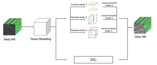
During the acquisition process, hyperspectral images (HSIs) are inevitably contaminated by mixed noise, which seriously affects the image quality. To improve the image quality, HSI denoising is a critical preprocessing step. In HSI denoising tasks, the method based on low-rank prior has achieved satisfying results. Among numerous denoising methods, the tensor nuclear norm (TNN), based on the tensor singular value decomposition (t-SVD), is employed to describe the low-rank prior approximately. Its calculation can be sped up by the fast Fourier transform (FFT). However, TNN is computed by the Fourier transform, which lacks the function of locating frequency. Besides, it only describes the low-rankness of the spectral correlations and ignores the spatial dimensions’ information. In this paper, to overcome the above deficiencies, we use the basis redundancy of the framelet and the low-rank characteristics of HSI in three modes. We propose the framelet-based tensor fibered rank as a new representation of the tensor rank, and the framelet-based three-modal tensor nuclear norm (F-3MTNN) as its convex relaxation. Meanwhile, the F-3MTNN is the new regularization of the denoising model. It can explore the low-rank characteristics of HSI along three modes that are more flexible and comprehensive. Moreover, we design an efficient algorithm via the alternating direction method of multipliers (ADMM). Finally, the numerical results of several experiments have shown the superior denoising performance of the proposed F-3MTNN model.

1. Introduction

Hyperspectral images (HSIs) can provide hundreds of continuous spectral bands, containing rich spatial and spectral information. They are used widely in many applications [1,2,3,4], including food safety, biomedicine, urban planning, cadastral investigation, industry, and so forth. However, during the acquisition process, due to unique physical designs and the limitations of the imaging mechanism, HSIs are inevitably contaminated by mixed noise [5,6]. This seriously reduces the image quality and bounds the precision of consequent processing tasks [1,7,8,9]. Thus, it is significant and challenging to denoise in the preprocessing steps for HSI applications.

Every spectral band of the HSIs is a gray-scale image measured by different wavelengths. From this perspective, numerous denoising methods applied to gray-scale images can be directly used in HSI denoising along the third dimension. However, these methods only utilize the structural information of each band individually and ignore the three-dimensional structural information of HSI. Therefore, the exploration of the spectral low-rankness of HSI is incomplete. To explore spectral characteristics in HSIs, some methods based on matrix low-rank prior [8,10,11,12,13,14,15,16,17,18] have been proposed and used widely and efficiently in HSI denoising tasks. The main idea is to unfold the HSI into a low-rank matrix by vectorizing spectral bands into columns. Minimizing the rank of the Casorati matrix is an efficient method for characterizing the low-rankness of HSI. However, it is unavoidable that the above matricization destroys the high order structures of HSIs [5]. With the development of tensor technology, more and more scholars have begun to pay attention to the low-rankness of tensor [19,20,21]. For example, NMoG uses LRMF to promote the low-rankness of the target HSIs [22]. In the past decades, a lot of research has been devoted to defining tensor ranks. The most typical definitions of the tensor rank are the CANDECOMP/PARAFAC(CP) rank [23,24] and the Tucker rank [25,26]. The CP rank is computed via the CP decomposition, which is defined as the minimum number of rank-one tensors required to express a tensor. Nevertheless, for a tensor, calculating the CP rank is NP-hard [27]. The Tucker rank is computed by unfolding the tensor to a matrix and computing the rank of the matrix based on the Tucker decomposition. However, the unfolding operation also destroys the spatial structure of tensors in Tucker decomposition [28].

Recently, the tensor singular value decomposition (t-SVD) has been proposed [29,30], induced by the tensor–tensor product (t-prod) [31], which is widely used in image restoration and denoising [32]. Then, the tensor tubal-rank and the tensor multi-rank have been defined based on t-SVD. They are accomplished using discrete Fourier transform (DFT). Due to the operation on the entire tensor, they can describe the low-rankness of tensors better. Similar to the matrix, minimizing the tensor rank function is NP-hard. The tensor nuclear norm (TNN) was developed as a convex approximation of the rank function of the tensors, which can solve this problem. TNN is directly defined on tensors and does not need the unfolding operation, which avoids losing the inherent information of tensors [33]. Meanwhile, t-SVD can be accomplished quickly by fast Fourier transform (FFT). Therefore, TNN is widely used in HSI denoising tasks.

However, TNN using DFT also has aspects not considered. Firstly, the Fourier transform can only calculate the magnitude of the frequency and lacks the function of locating frequency. Secondly, there are many transformations that can make the rank lower in the transform domain. It has been found that the tubal-rank could be smaller when it is accomplished with a suitable unitary transform [34]. In addition, it has been proven that a tensor can be recovered exactly when it has a sufficiently low tubal-rank and the corrupted entries are sufficiently sparse [34]. Naturally, if there is a transformation to make the rank of the transformed tensor lower, this is of great significance for more effective image denoising. Besides the Fourier transform, there are numerous invertible transformations that can be used in the tensor decomposition scheme [28], for example, the discrete cosine transform (DCT) and the Haar wavelet transform.

Among these transformations that can be used within the t-SVD framework, we adopt the tight wavelet frame (framelet). Compared with the Fourier transform, the framelet transform has the following advantages. Firstly, the framelet can link the frequency intensity information with the position information, which solves the shortcomings of the Fourier transform to a certain extent. Secondly, the framelet is redundant [35]. Consequently, the representation of each fiber is sparse. For this, we conduct experiments to verify this result. One can see Section 3 for details. As a result, we find that the framelet is a suitable transformation, which can make the rank of the transformed tensor lower, and we can minimize the TNN based on the framelet to solve the problem in HSI denoising tasks.

Additionally, the traditional tensor rank based on t-SVD only transforms along the spectral dimension, which mainly describes the low-rankness of the spectral correlations and inevitably ignores the spatial information. From this perspective, we need to deal with various correlations along three modes of HSI. However, the traditional tensor rank based on t-SVD lacks the ability and flexibility [5]. To remedy this defect and improve noise reduction performance, we use three-modal t-SVD based on framelet transform to define the tensor rank and the framelet-based three-modal TNN (F-3MTNN) as its convex relaxation. It is more flexible and precise to represent the low-rankness characterization of the HSI. The details are introduced in Section 3.

The main contributions are listed as follows: (1) Taking full advantage of the redundancy of the framelet transform and the low-rankness of the framelet-based transformed tensor, we propose the framelet-based TNN, which is more conducive to exploring low-rankness for denoising tasks; afterwards, to overcome the shortage of the exploration in the low-rank characteristics of three dimensions, we propose the F-3MTNN model, which is more flexible, accurate and complete in dimensionality; (2) Based on the above, we proposed a framelet-based TNN minimization model and applied it to HSI denoising. To solve the proposed model, based on the ADMM algorithm, a fast algorithm is built [36].

2. Preliminaries

2.1. Notations and Definitions

In this section, some related operations and definitions are generalized [5]. Generally, we denote the third-order tensor as $\mathcal{A}\in R^{n_1\times n_2\times n_3}$. Its $(i,j,s)$th element is denoted as $\mathcal{A}(i,j,s)$, following the terminology used in MATLAB. Given a tensor $\mathcal{A}\in R^{n_1\times n_2\times n_3}$, the transformed tensor via FFT along the third mode is ${\overline{\mathcal{A}}}_k$, that is, ${\overline{\mathcal{A}}}_k=fft(\mathcal{A},\left[\right],3)$. Certainly, we can compute $\mathcal{A}$ via $\mathcal{A}=ifft({\overline{\mathcal{A}}}_k,\left[\right],k)$. The kth-modal permutation of $\mathcal{A}$ is defined as ${\mathcal{A}}_k=permute(\mathcal{A},k),k=1,2,3$, where the m-th third-modal slice of ${\mathcal{A}}_k$ is the m-th kth-modal slice of $\mathcal{A}$, that is, $\mathcal{A}(i,j,s)={\mathcal{A}}_1(j,s,i)={\mathcal{A}}_2(s,i,j)={\mathcal{A}}_3(i,j,s)$. Naturally, the inverse operation is $\mathcal{A}=ipermute({\mathcal{A}}_k,k)$. ${\parallel ·\parallel }_F$ is the Frobenius norm, which is defined as ${\parallel \mathcal{A}\parallel }_F:=({\sum }_{i,j,s}{\left|\mathcal{A}(i,j,s)\right|}^2{)}^{\frac{1}{2}}$. ${\parallel ·\parallel }_1$ is the $l_1$ norm, which is defined as ${\parallel \mathcal{A}\parallel }_1:={\sum }_{i,j,s}\left|\mathcal{A}(i,j,s)\right|$.

2.2. Framelet

The tight frame $X\subset L_2\left(R\right)$ of $L_2\left(R\right)$ is defined as:

$${\parallel f\parallel }_2^2=\sum _{g\in X}{\left|\langle f,g\rangle \right|}^2,\forall f\in L_2\left(R\right),$$

where $\langle ·,·\rangle$ is the inner product in $L_2\left(R\right)$ and ${\parallel ·\parallel }_2={\langle ·,·\rangle }^{\frac{1}{2}}$.

A wavelet system $X\left(\mathsf{\Psi }\right)$ is the collection of dilations and shifts of a finite set $\mathsf{\Psi }\subset L_2\left(R\right)$, that is,

$$X\left(\mathsf{\Psi }\right)=\{2^{k/2}\psi (2^{k}x-j):\psi \in \mathsf{\Psi },k,j\in Z\},$$

then $\psi$ is called a framelet if $X\left(\mathsf{\Psi }\right)$ is also a tight frame for $L_2\left(R\right)$.

In the actual application of image processing, to facilitate calculations, the framelet transform can be represented as a decomposition operator. For example, given a vector $a\in R^n$, its transformed vector $\widehat{a}$ can be calculated by $\widehat{a}=Wa\in R^{wn}$, where $W\in R^{wn\times n}$ is the framelet transform matrix ($w=(n-1)l+1$, n is the number of filters and l is the number of levels). The generating process of W is detailed in [35,37], and will not be repeated here.

2.3. Problem Formulation

HSIs are degraded by different types of mixed noises. These noises are usually composed of Gaussian noise, impulse noise, striped noise, and so on [38]. It is assumed that the original hyperspectral data are $\mathcal{X}\in R^{n_1\times n_2\times n_3}$, where $n_1\times n_2$ is the spatial size and $n_3$ is the spectral size of HSI. Then, the degradation model can be presented as follows:

$$\mathcal{X}=\mathcal{L}+\mathcal{N}+\mathcal{S},$$

(1)

where $\mathcal{X},\mathcal{L},\mathcal{N},\mathcal{S}\in R^{n_1\times n_2\times n_3}$; $\mathcal{L}$ is the clean HSI without noise; $\mathcal{X}$ is the original HSI; $\mathcal{N}$ represents the Gaussian noise; $\mathcal{S}$ represents the sparse noise composed by impulse noise, striped noise, and so forth.

Based on the degradation model (1), HSI denoising obtains the original clear HSI through observation data. Obviously, it is a serious ill-posed problem. Therefore, taking advantage of the prior information of HSI, the regularized denoising framework can be used to solve this problem. It can be presented in a concise form:

$$\begin{array}{c}\hfill arg\underset{\mathcal{L},\mathcal{N},\mathcal{S}}{min}rank\left(\mathcal{L}\right)+{\lambda }_1{\parallel \mathcal{N}\parallel }_F^2+{\lambda }_2{\parallel \mathcal{S}\parallel }_{1}s.t.\mathcal{X}=\mathcal{L}+\mathcal{N}+\mathcal{S},\end{array}$$

(2)

where $rank(·)$ represents the rank of the tensor; ${\lambda }_1$ and ${\lambda }_2$ are regularization parameters.

2.4. DFT-Based Tensor Fibered Rank

As mentioned above, the low-rank prior is an essential part of the regularized denoising framework. To represent $rank(·)$ more accurately, the tensor fibered rank is proposed in [5].

Definition 1.

(DFT-based tensor fibered rank [5]). Given a tensor $\mathcal{A}\in R^{n_1\times n_2\times n_3}$, the fibered rank of $\mathcal{A}$ is a vector, denoted as $ran{k}_f\left(\mathcal{A}\right)$, in which the kth element is the number of nonzero fibers of $\overline{{\mathcal{S}}_k}$, where $\overline{{\mathcal{S}}_k}$ comes from the SVD of $\overline{{\mathcal{A}}_k}$: $\overline{{\mathcal{A}}_k}=\overline{{\mathcal{U}}_k}·\overline{{\mathcal{S}}_k}·\overline{{\mathcal{V}}_k^T}$.

The Definition 1 is based on the Fourier transform. In [5], the DFT-based characterization of low-rankness in tensors played an important role in HSI denoising.

3. Proposed Model

3.1. Framelet-Based Tensor Fibered Rank and Corresponding Three-Modal TNN

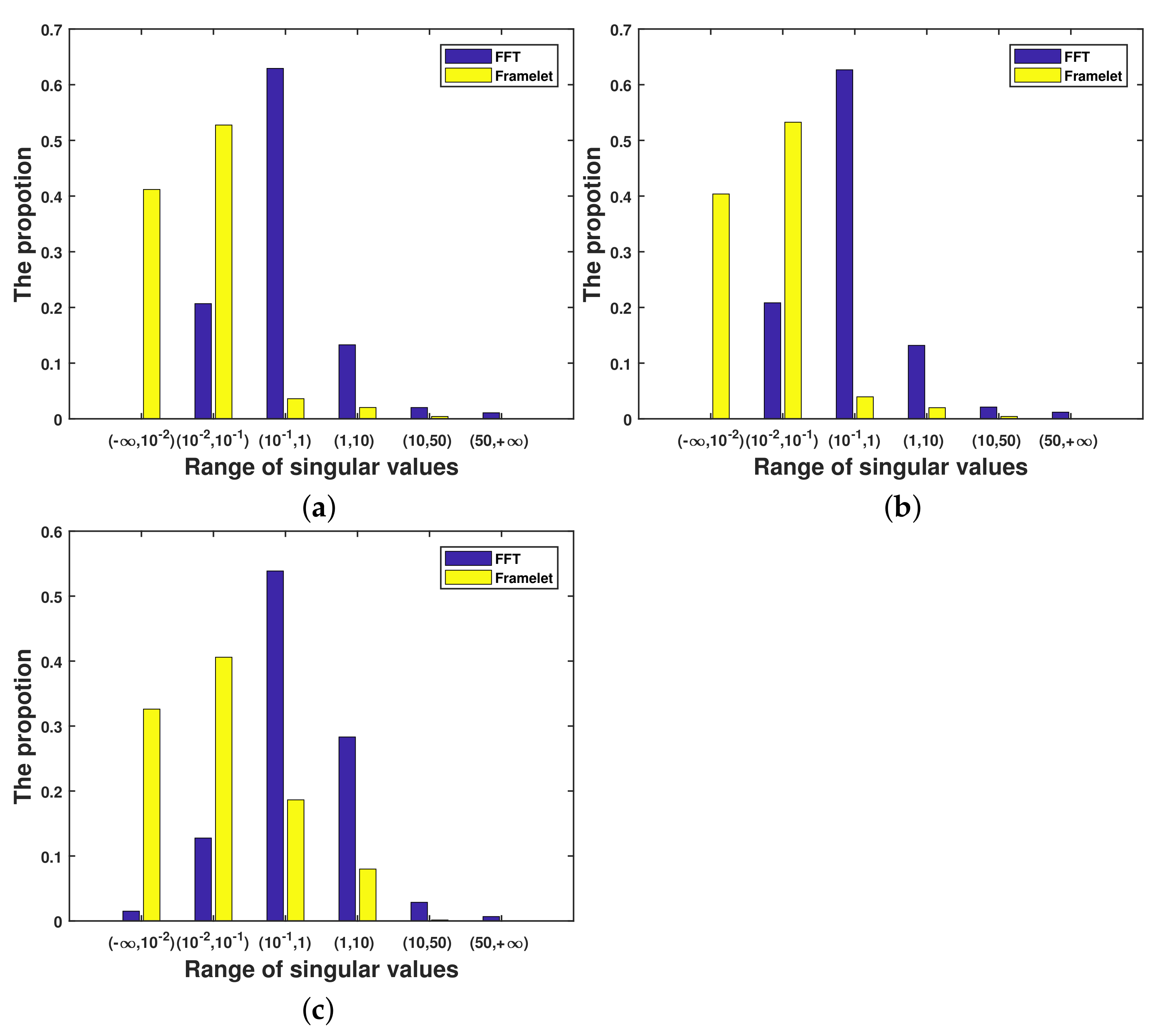
Definition 1 is used to describe the rank of tensors, which characterizes the correlations of different dimensions of HSIs flexibly. However, it is more important that the framelet will bring in redundancy, which means the transformed tensor has a lower rank. As an example, we use two datasets, which are the Pavia City Center dataset and the USGS Indian pines dataset to compare the fibered rank after FFT transformation and framelet transformation. Their sizes are $200\times 200\times 80$ and $145\times 145\times 224$, respectively. Since each transformed tensor’s slice has numerous small singular values for real image data [28], we only keep the singular values that are greater than the truncation parameter for discussion. The result is shown in

Table 1. The mean value of fibered rank for three orders by using a different transform.

Data	$\mathit{\tau }$	Transformation	The First Mode	The Second Mode	The Third Mode
Pavia	0.04	FFT	78	78	188
		Framelet	13	13	70
	0.05	FFT	75	75	185
		Framelet	10	10	65
Indian	0.04	FFT	16	16	106
		Framelet	3	3	42
	0.05	FFT	16	16	105
		Framelet	3	3	40

. The result shows that the transformed tensor via framelet has a lower fibered rank than that via the Fourier transformation. As a result, we can believe that using the framelet-based tensor rank to constrain low-rank prior will have a better effect in HSI denoising.

Accordingly, we propose the new tensor fibered rank based on the framelet transform. At first, similar to the previous notation, we denote the transformed tensor by the framelet along the kth mode as:

$${\widehat{\mathcal{A}}}_k=W_k{\mathcal{A}}_k,$$

where $W_k\in R^{w{n}_k\times n_k}$ is the framelet transform matrix. According to the unitary extension principle (UEP) [39] property, we have ${\mathcal{A}}_k=W^T{\widehat{\mathcal{A}}}_k$.

Then, we define the framelet-based tensor fibered rank.

Definition 2.

(tensor fibered rank [5]). Given a tensor $\mathcal{A}\in R^{n_1\times n_2\times n_3}$, the fibered rank of $\mathcal{A}$ is a vector, denoted as $ran{k}_f^F\left(\mathcal{A}\right)$, whose kth element is the number of nonzero fibers of $\widehat{{\mathcal{S}}_k}$, where $\widehat{{\mathcal{S}}_k}$ satisfies $\widehat{{\mathcal{A}}_k}$: $\widehat{{\mathcal{A}}_k}=\widehat{{\mathcal{U}}_k}·\widehat{{\mathcal{S}}_k}·\widehat{{\mathcal{V}}_k^T}$.

To demonstrate the superiority of the representation for tensor low-rankness, we use the Pavia City Center dataset to conduct some empirically numerical analyses. For the frontal slices in each transformed tensor, we count the number of the singular values in each magnitude interval. The ratio is shown in Figure 1. Compared with the original tensor and the transformed tensor via FFT, we find that the singular values of the transformed tensor via framelet are mostly gathered in the smaller interval, which means the transformed tensor via framelet has a lower fibered rank than that via the Fourier transformation.

However, it is NP-hard to minimize the framelet-based tensor fibered rank. The following framelet-based three-modal TNN (F-3MTNN) is defined as the convex relaxation of the framelet-based tensor fibered rank.

Definition 3.

(F-3MTNN) The F-3MTNN of a tensor $\mathcal{A}\in R^{n_1\times n_2\times n_3}$, denoted as ${\parallel \mathcal{A}\parallel }_{F-3MTNN}$, is defined as:

$${\parallel \mathcal{A}\parallel }_{F-3MTNN}:=\sum _{k=1}^3{w}_k{\parallel \mathcal{A}\parallel }_{TN{N}_k}^F,$$

where $w_k⩾0(k=1,2,3)$, ${\sum }_{k=1}^3{w}_k=1$ and ${\parallel \mathcal{A}\parallel }_{TN{N}_k}^F$ is the framelet-based kth-modal TNN of $\mathcal{A}$, defined as:

$${\parallel \mathcal{A}\parallel }_{TN{N}_k}^F:=\sum _{i=1}^{w{n}_k}{\parallel {\left(\widehat{{\mathcal{A}}_k}\right)}^{\left(i\right)}\parallel }_{*},$$

where ${\parallel ·\parallel }_{*}$ is the matrix nuclear norm and ${\left(\widehat{{\mathcal{A}}_k}\right)}^{\left(i\right)}$ is the ith third-modal slice of $\widehat{{\mathcal{A}}_k}$, that is, ${\left(\widehat{{\mathcal{A}}_k}\right)}^{\left(i\right)}=\widehat{{\mathcal{A}}_k}(:,:,i)$.

The F-3MTNN is a convex envelope of the $l_1$ norm of the $ran{k}_f^F(·)$. The HSI is low-rank in both spatial and spectral dimensions. Based on this data characteristic, F-3MTNN has the ability to explore the correlations along different modes flexibly and simultaneously.

3.2. Proposed Denoising Model

According to the advantages of the framelet-based tensor fibered rank, the HSI denoising model (2) is rewritten as:

$$\begin{array}{c}\hfill arg\underset{\mathcal{L},\mathcal{N},\mathcal{S}}{min}ran{k}_f^F\left(\mathcal{L}\right)+{\lambda }_1{\parallel \mathcal{N}\parallel }_F^2+{\lambda }_2{\parallel \mathcal{S}\parallel }_{1}s.t.\mathcal{X}=\mathcal{L}+\mathcal{N}+\mathcal{S}.\end{array}$$

(3)

As mentioned earlier, it is an NP-hard problem to minimize the tensor fibered rank. Based on F-3MTNN, the proposed model (3) can be represented as:

$$\begin{array}{c}\hfill arg\underset{\mathcal{L},\mathcal{N},\mathcal{S}}{min}{\parallel \mathcal{L}\parallel }_{F-3MTNN}+{\lambda }_1{\parallel \mathcal{N}\parallel }_F^2+{\lambda }_2{\parallel \mathcal{S}\parallel }_{1}s.t.\mathcal{X}=\mathcal{L}+\mathcal{N}+\mathcal{S},\end{array}$$

(4)

that is,

$$\begin{array}{c}\hfill arg\underset{\mathcal{L},\mathcal{N},\mathcal{S}}{min}\sum _{k=1}^3{w}_k\parallel {\mathcal{L}}_k{\parallel }_{TN{N}_k}^F+{\lambda }_1{\parallel \mathcal{N}\parallel }_F^2+{\lambda }_2{\parallel \mathcal{S}\parallel }_{1}s.t.\mathcal{X}=\mathcal{L}+\mathcal{N}+\mathcal{S},\end{array}$$

(5)

where $w_k⩾0(k=1,2,3)$ and ${\sum }_{k=1}^3{w}_k=1$.

Unlike the traditional t-SVD using the Fourier transform, the proposed model uses the framelet transform and explores the low-rank characteristics of HSI more accurately, for the reason that the tensor fibered rank after the framelet transform is lower, and the framelet transform has redundancy. In addition, F-3MTNN can maintain the advantage in characterizing low-rankness as the convex approximation of the framelet-based tensor fibered TNN.

3.3. Optimization Procedure

Based on ADMM, we introduce three auxiliary variables ${\mathcal{Z}}_k(k=1,2,3)$ to solve (5). Then, we reformulate (5) as:

$$\begin{array}{cc}\hfill arg\underset{\mathcal{L},{\mathcal{Z}}_k,\mathcal{N},\mathcal{S}}{min}\sum _{k=1}^3& w_k{\parallel {\mathcal{Z}}_k\parallel }_{TN{N}_k}^F+{\lambda }_1{\parallel \mathcal{N}\parallel }_F^2+{\lambda }_2{\parallel \mathcal{S}\parallel }_1\hfill \\ \hfill & s.t.\mathcal{X}=\mathcal{L}+\mathcal{N}+\mathcal{S},\mathcal{L}={\mathcal{Z}}_k,k=1,2,3.\hfill \end{array}$$

(6)

Based on the ALM method, we rewrite (6) as:

$$\begin{array}{cc}\hfill arg\underset{\mathcal{L},\mathcal{Z},\mathcal{N},\mathcal{S}}{min}& \sum _{k=1}^3\{w_k{\parallel {\mathcal{Z}}_k\parallel }_{TN{N}_k}^F+\frac{{\mu }_k}{2}{\parallel \mathcal{L}-{\mathcal{Z}}_k\parallel }_F^2+\langle {\mathcal{Y}}_k,\mathcal{L}-{\mathcal{Z}}_k\rangle \}\hfill \\ \hfill & +{\lambda }_1{\parallel \mathcal{N}\parallel }_F^2+{\lambda }_2{\parallel \mathcal{S}\parallel }_1+\frac{\beta }{2}{\parallel \mathcal{X}-(\mathcal{L}+\mathcal{N}+\mathcal{S})\parallel }_F^2\hfill \\ \hfill & +\langle \mathcal{M},\mathcal{X}-(\mathcal{L}+\mathcal{N}+\mathcal{S})\rangle ,\hfill \end{array}$$

(7)

where ${\mathcal{Y}}_k(k=1,2,3)$ and $\mathcal{M}$ are the Lagrange multipliers; ${\mu }_k(k=1,2,3)$ and $\beta$ are the penalty parameters. In the pth iteration, the solution of (7) in the $p+1$th iteration can be divided into the following subproblems:

(a) The subproblem of $\mathcal{L}$:

$$\begin{array}{cc}\hfill {\mathcal{L}}^{p+1}& =arg\underset{\mathcal{L}}{min}\sum _{k=1}^3\{\frac{{\mu }_k}{2}{\parallel \mathcal{L}-{\mathcal{Z}}_k^p\parallel }_F^2+\langle {\mathcal{Y}}_k,\mathcal{L}-{\mathcal{Z}}_k^p\rangle \}\hfill \\ \hfill & +\frac{\beta }{2}{\parallel \mathcal{X}-(\mathcal{L}+{\mathcal{N}}^p+{\mathcal{S}}^p)\parallel }_F^2+\langle \mathcal{M},\mathcal{X}-(\mathcal{L}+{\mathcal{N}}^p+{\mathcal{S}}^p)\rangle \hfill \\ \hfill & =arg\underset{\mathcal{L}}{min}\sum _{k=1}^3\frac{{\mu }_k}{2}{\parallel \mathcal{L}+\frac{{\mathcal{Y}}_k}{{\mu }_k}-{\mathcal{Z}}_k^p\parallel }_F^2+\frac{\beta }{2}{\parallel \mathcal{L}+{\mathcal{N}}^p+{\mathcal{S}}^p-\mathcal{X}-\frac{\mathcal{M}}{\beta }\parallel }_F^2.\hfill \end{array}$$

(8)

Then, we have:

$$\begin{array}{c}\hfill {\mathcal{L}}^{p+1}=\frac{{\sum }_{k=1}^3{\mu }_k({\mathcal{Z}}_k^p-\frac{{\mathcal{Y}}_k}{{\mu }_k})+\beta (\mathcal{X}+\frac{\mathcal{M}}{\beta }-{\mathcal{N}}^p-{\mathcal{S}}^p)}{{\sum }_{k=1}^3{\mu }_k+\beta }.\end{array}$$

(9)

(b) The subproblem of ${\mathcal{Z}}_k$

$$\begin{array}{cc}\hfill {\mathcal{Z}}_k^{p+1}& =arg\underset{{\mathcal{Z}}_k}{min}{w}_k{\parallel {\mathcal{Z}}_k\parallel }_{TN{N}_k}^F+\frac{{\mu }_k}{2}{\parallel {\mathcal{L}}^{p+1}-{\mathcal{Z}}_k\parallel }_F^2+\langle {\mathcal{Y}}_k,{\mathcal{L}}^{p+1}-{\mathcal{Z}}_k\rangle \hfill \\ \hfill & =arg\underset{{\mathcal{Z}}_k}{min}{w}_k{\parallel {\mathcal{Z}}_k\parallel }_{TN{N}_k}^F+\frac{{\mu }_k}{2}{\parallel {\mathcal{Z}}_k-{\mathcal{L}}^{p+1}-\frac{{\mathcal{Y}}_k}{{\mu }_k}\parallel }_F^2.\hfill \end{array}$$

(10)

Based on [40], we can obtain the result of (10) by the singular value shrinkage operator as follows. The details are presented in Algorithm 1.

$$\begin{array}{c}\hfill {\mathcal{Z}}_k^{p+1}={\mathcal{D}}_{w_k/{\mu }_k}({\mathcal{L}}^{p+1}+\frac{{\mathcal{Y}}_k}{{\mu }_k}).\end{array}$$

(11)

Algorithm 1. Framelet-besed kth-modal singular value shrinkage operator.

Input:$\mathcal{A}\in R^{n_1\times n_2\times n_3}$, $\tau$, $W\in R^{w{n}_k\times n_k}$, w and k

Output:$D_{\tau }\left(\mathcal{A}\right)$

1: ${\widehat{\mathcal{A}}}_k=W{\mathcal{A}}_k$

2: for $i=1,...,w{n}_k$do

3:  $[\widehat{U},\widehat{\Sigma },\widehat{V^T}]=SVD\left({\widehat{{\mathcal{A}}_k}}^{\left(i\right)}\right)$

4:  ${\widehat{{\mathcal{A}}_k}}^{\left(i\right)}=\widehat{U}·{(\widehat{\Sigma }-\tau )}_{+}·\widehat{V^T}$

5: end for

6: Compute $D_{\tau }\left(\mathcal{A}\right)=W^T\widehat{{\mathcal{A}}_k}.$

(c) The subproblem of $\mathcal{N}$

$$\begin{array}{cc}\hfill {\mathcal{N}}^{p+1}& =arg\underset{\mathcal{N}}{min}{\lambda }_1{\parallel \mathcal{N}\parallel }_F^2+\frac{\beta }{2}{\parallel \mathcal{X}-({\mathcal{L}}^{p+1}+\mathcal{N}+{\mathcal{S}}^p)\parallel }_F^2+\langle \mathcal{M},\mathcal{X}-({\mathcal{L}}^{p+1}+\mathcal{N}+{\mathcal{S}}^p)\rangle \hfill \\ \hfill & =arg\underset{\mathcal{N}}{min}{\lambda }_1{\parallel \mathcal{N}\parallel }_F^2+\frac{\beta }{2}{\parallel \mathcal{N}+{\mathcal{L}}^{p+1}+{\mathcal{S}}^p-\mathcal{X}-\frac{\mathcal{M}}{\beta }\parallel }_F^2.\hfill \end{array}$$

(12)

Then we have:

$$\begin{array}{c}\hfill {\mathcal{N}}^{p+1}=\frac{\beta (\mathcal{X}+\frac{\mathcal{M}}{\beta }-{\mathcal{L}}^{p+1}-{\mathcal{S}}^p)}{2{\lambda }_1+\beta }.\end{array}$$

(13)

(d) The subproblem of $\mathcal{S}$

$$\begin{array}{cc}\hfill {\mathcal{S}}^{p+1}& =arg\underset{\mathcal{S}}{min}{\lambda }_2{\parallel \mathcal{S}\parallel }_1+\frac{\beta }{2}{\parallel \mathcal{X}-({\mathcal{L}}^{p+1}+{\mathcal{N}}^{p+1}+\mathcal{S})\parallel }_F^2+\langle \mathcal{M},\mathcal{X}-({\mathcal{L}}^{p+1}+{\mathcal{N}}^{p+1}+\mathcal{S})\rangle \hfill \\ \hfill & =arg\underset{\mathcal{S}}{min}{\lambda }_2{\parallel \mathcal{S}\parallel }_1+\frac{\beta }{2}{\parallel {\mathcal{N}}^{p+1}+{\mathcal{L}}^{p+1}+\mathcal{S}-\mathcal{X}-\frac{\mathcal{M}}{\beta }\parallel }_F^2\hfill \\ \hfill & =arg\underset{\mathcal{S}}{min}{\lambda }_2{\parallel \mathcal{S}\parallel }_1+\frac{\beta }{2}{\parallel \mathcal{S}-(\mathcal{X}+\frac{\mathcal{M}}{\beta }-{\mathcal{L}}^{p+1}-{\mathcal{N}}^{p+1})\parallel }_F^2.\hfill \end{array}$$

(14)

The optimization result can be immediately obtained as follows:

$$\begin{array}{c}\hfill {\mathcal{S}}^{p+1}={\Re }_{{\lambda }_2/\beta }(\mathcal{X}+\frac{\mathcal{M}}{\beta }-{\mathcal{L}}^{p+1}-{\mathcal{N}}^{p+1}),\end{array}$$

(15)

where ${\Re }_{{\lambda }_2/\beta }(·)$ is the soft-thresholding (shrinkage) operator in [41].

After solving the subproblems, the Lagrangian multipliers ${\mathcal{Y}}_k(k=1,2,3)$ and $\mathcal{M}$ can be updated as follows:

$$\begin{array}{c}\hfill \left\{\begin{array}{cc}\hfill & {\mathcal{Y}}_k^{p+1}={\mathcal{Y}}_k^p+{\mu }_k^p({\mathcal{L}}^{p+1}-{\mathcal{Z}}_k^{p+1})\hfill \\ \hfill & {\mathcal{M}}^{p+1}={\mathcal{M}}^p+{\beta }^p(\mathcal{X}-{\mathcal{L}}^{p+1}-{\mathcal{S}}^{p+1}-{\mathcal{N}}^{p+1}).\hfill \end{array}\right.\end{array}$$

(16)

The solving algorithm can be acquired in Algorithm 2.

Algorithm 2. HSI Denoising via the F-3MTNN minimization.

Input: The observed HSI $\mathcal{X}\in R^{n_1\times n_2\times n_3}$, $w_k(k=1,2,3)$, ${\lambda }_1$, ${\lambda }_2$, $\rho$, $\tau$ and $\epsilon$.

Output: The denoised HSI $\mathcal{L}$

1: Initialize: ${\mathcal{L}}^0$ = ${\mathcal{N}}^0$ = ${\mathcal{S}}^0$ = ${\mathcal{Z}}_k^0$, ${\mu }_k=\beta =0$, ${\mathcal{Y}}_k=\mathcal{M}=\mathcal{O}$, $\rho =1.2$, $\epsilon ={10}^{-6}$

2: Repeat until convergence:

Update ${\mathcal{L}}^{p+1}$ by (9)

Update ${\mathcal{Z}}_k^{p+1}$ by (11)

Update ${\mathcal{N}}^{p+1}$ by (13)

Update ${\mathcal{S}}^{p+1}$ by (15)

Update ${\mathcal{Y}}^{p+1}$ and ${\mathcal{M}}^{p+1}$ by (16)

Update ${\mu }^{p+1}$ and ${\beta }^{p+1}$: ${\mu }^{p+1}=\rho {\mu }^p$, ${\beta }^{p+1}=\rho {\beta }^p$; $p=p+1$

3: Check the convergence conditions

$max\{\parallel {\mathcal{L}}^{p+1}-{\mathcal{L}}^p{\parallel }_{\infty },\parallel \mathcal{X}-{\mathcal{L}}^{p+1}-{\mathcal{N}}^{p+1}-{\mathcal{S}}^{p+1}{\parallel }_{\infty },\parallel {\mathcal{L}}^{p+1}-{\mathcal{Z}}_k^{p+1}{\parallel }_{\infty }\}⩽\epsilon$

4. Experimental Results

To test the performance of our denoising model, the experiments were conducted on two simulated datasets and two real datasets. For all the testing HSIs, we normalized them to [0,1] band by band. To evaluate the performance of our model comprehensively, we chose seven methods for the comparison: (1) LRTA [42]; (2) BM4D [12]; (3) LRMR [13]; (4) LRTDTV [43]; (5) L1HyMixDe [44]; (6) LRTDGS [45]; (7) 3DTNN [5]. Since the LRTA and BM4D methods are only used to remove Gaussian noise, we pre-processed the datasets by the RPCA restoration method before implementing them.

We set all parameters according to the original codes or authors’ suggestions in their articles. The equipment included laptops of 16 GB RAM, Intel(R) Core(TM) i7-10750H CPU, @ 2.60 GHz, with MATLAB R2017a.

4.1. Experiments on Simulated Datasets

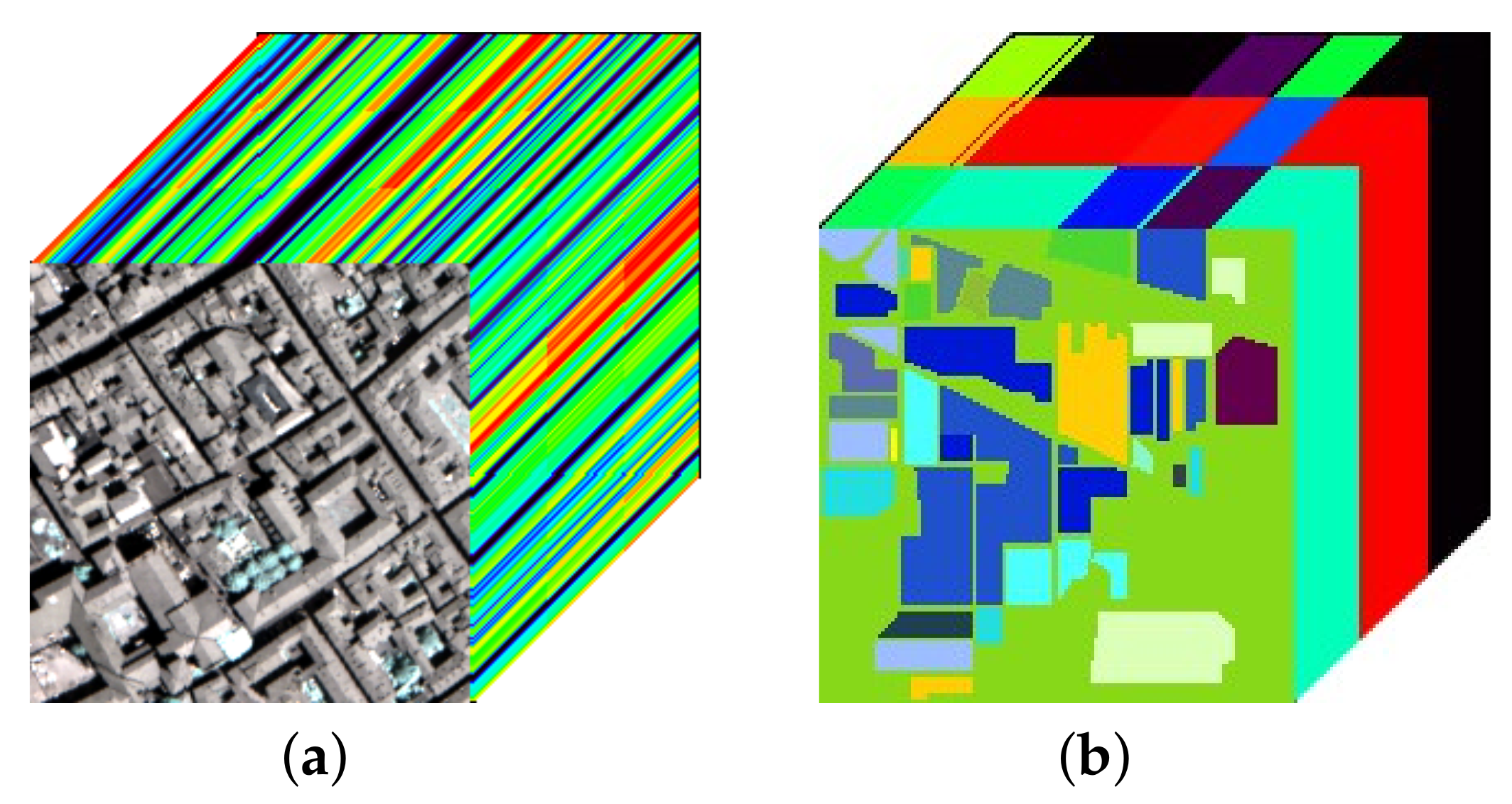
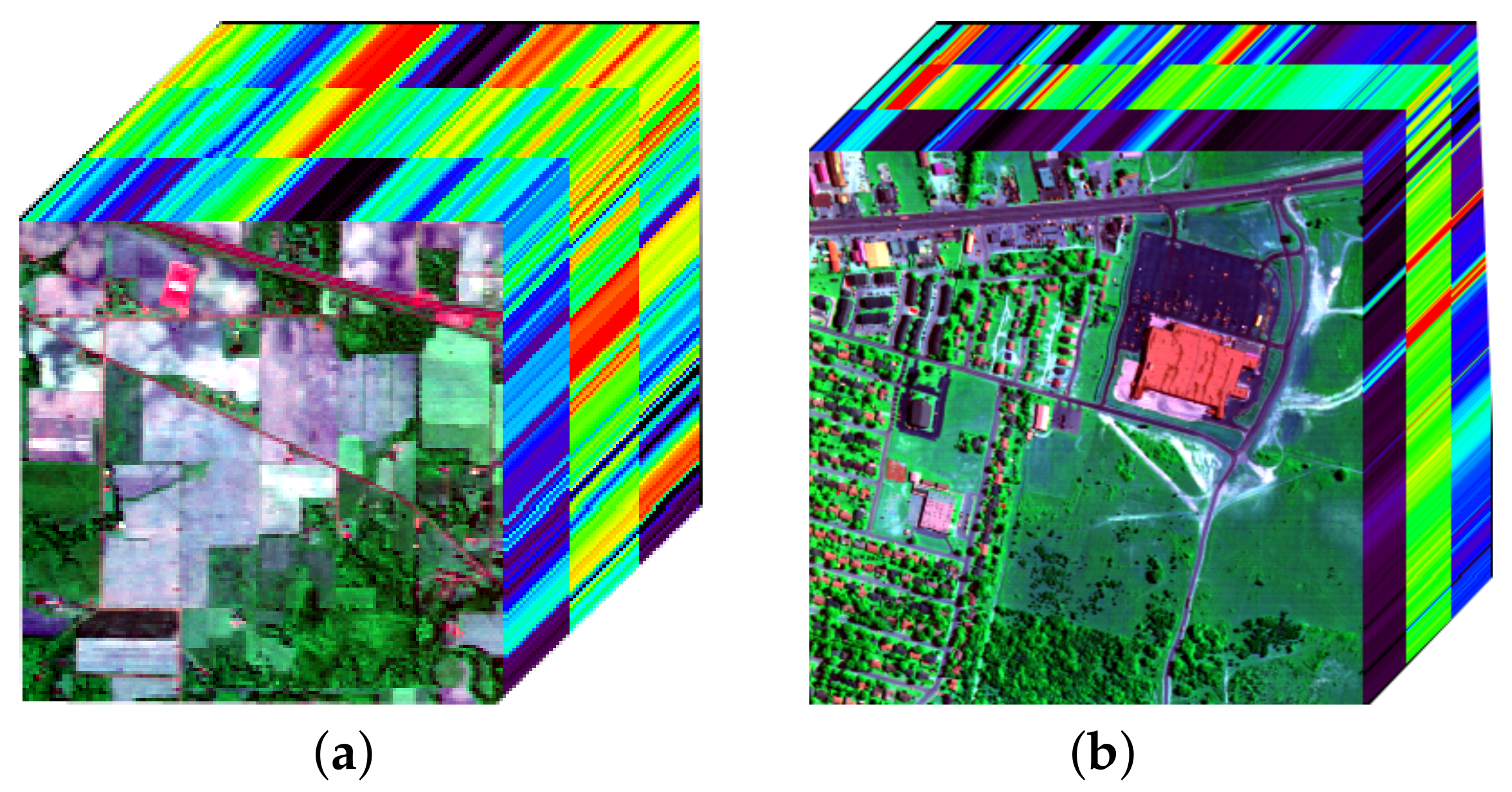
In this subsection, we built and performed some experiments on two simulated datasets, including a subimage of Pavia City Center dataset [46] (abbreviated as dataset-1), the size of which was $200\times 200\times 80$, and a subimage of USGS Indian pines dataset [47] (abbreviated as dataset-2), the size of which was $145\times 145\times 224$. Figure 2a,b lists the two selected HSIs.

We choose three indices to measure the performance of the denoising models. They are the mean of peak signal-to-noise rate (MPSNR), the mean of structural similarity (MSSIM), and the spectral angle mapping (SAM).

To simulate the real situation as realistically as possible, we added several kinds of mixed noise to the HSIs, consisting of Gaussian noise, impulse noise, deadline noise and stripe noise in different levels, which made the result more descriptive and effective. We made comparisons of both visual observation and quantitative indicators.

Table 2. The details of the eight noise cases.

Noise	Gaussian Noise	Impulse Noise	Deadline Noise	Stripe Noise
Case 1	mean value = 0, variance = 0.1	percentage = 0.2	\	\
Case 2	mean value = 0, variance = 0.15	percentage = 0.2	\	\
Case 3	mean value = 0, variance = 0.1	percentage = 0.1	\	\
Case 4	mean value = 0, variance = 0.1	percentage = 0.3	\	\
Case 5	mean value = 0, variance ∼ U(0.05, 0.15)	percentage = 0.2	\	\
Case 6	mean value = 0, variance ∼ U(0.1, 0.2)	percentage = 0.2	\	\
Case 7	mean value = 0	percentage = 0.3	10% of the bands	\
	variance = 0.1		number ∼ U(1, 4)	\
Case 8	mean value = 0	percentage = 0.3	10% of the bands	10% of the bands
	variance = 0.1		number ∼ U(1, 4)	number ∼ U(20, 40)

Note: The number means the number of deadling noise or stripe noise in a band.

lists the specific conditions of the intensity of various noises in eight noise cases:

4.1.1. Pavia City Center Dataset

(A) Visual Quality Comparison

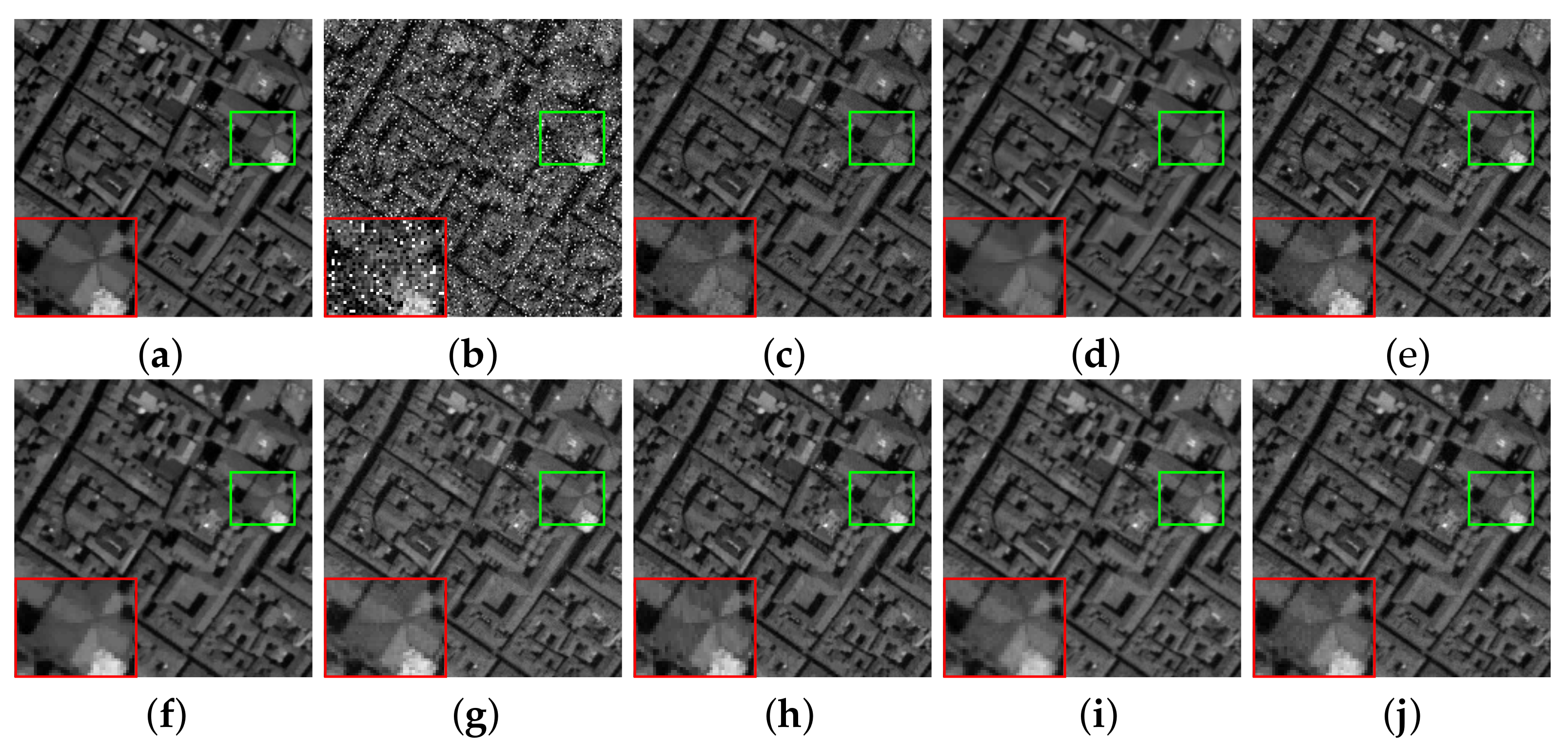
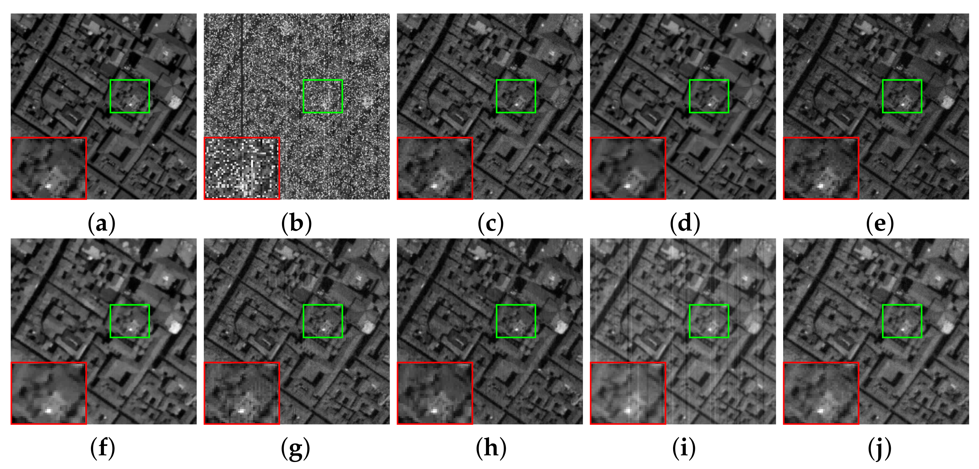
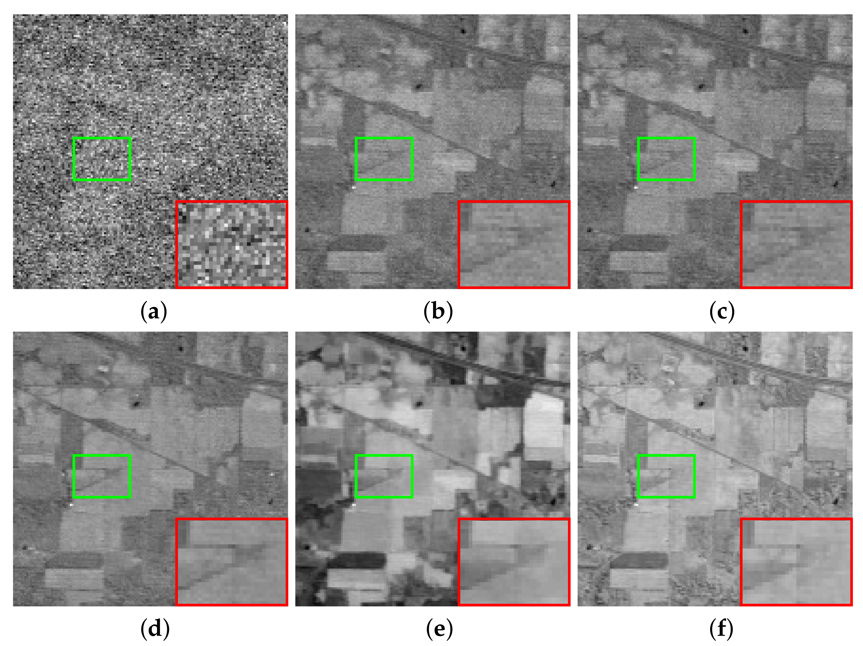
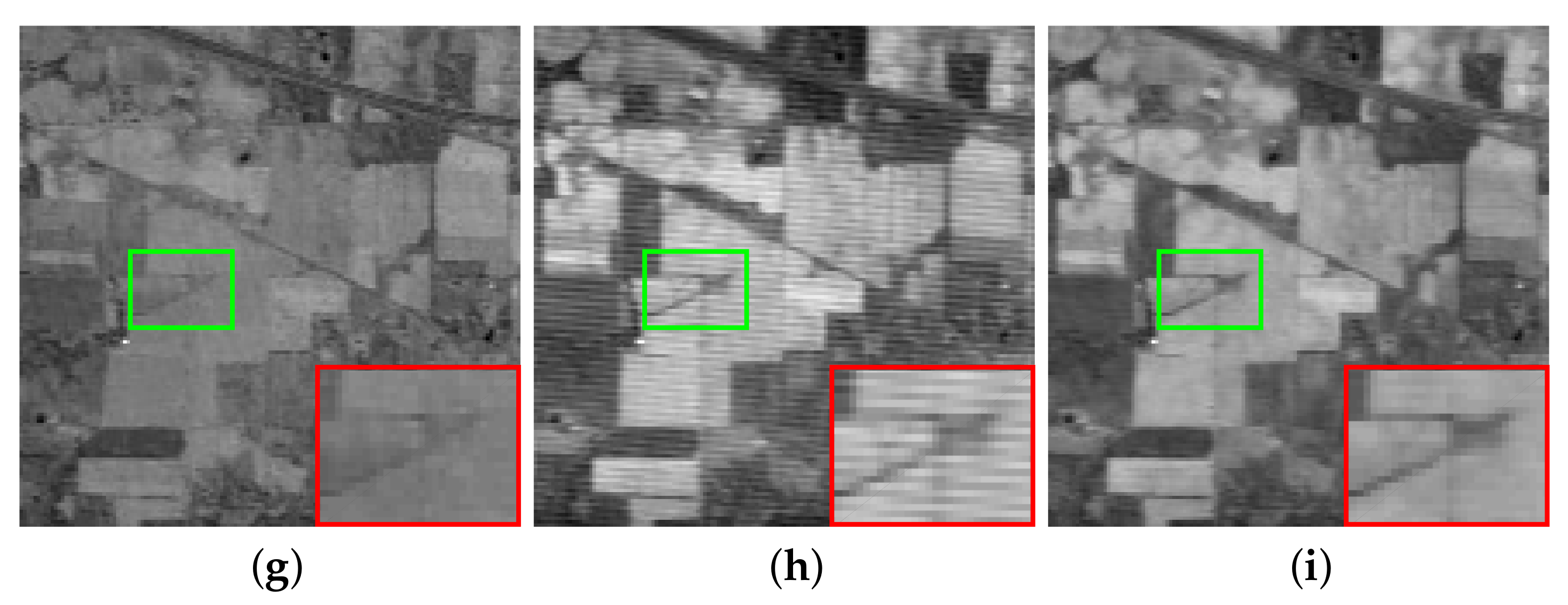
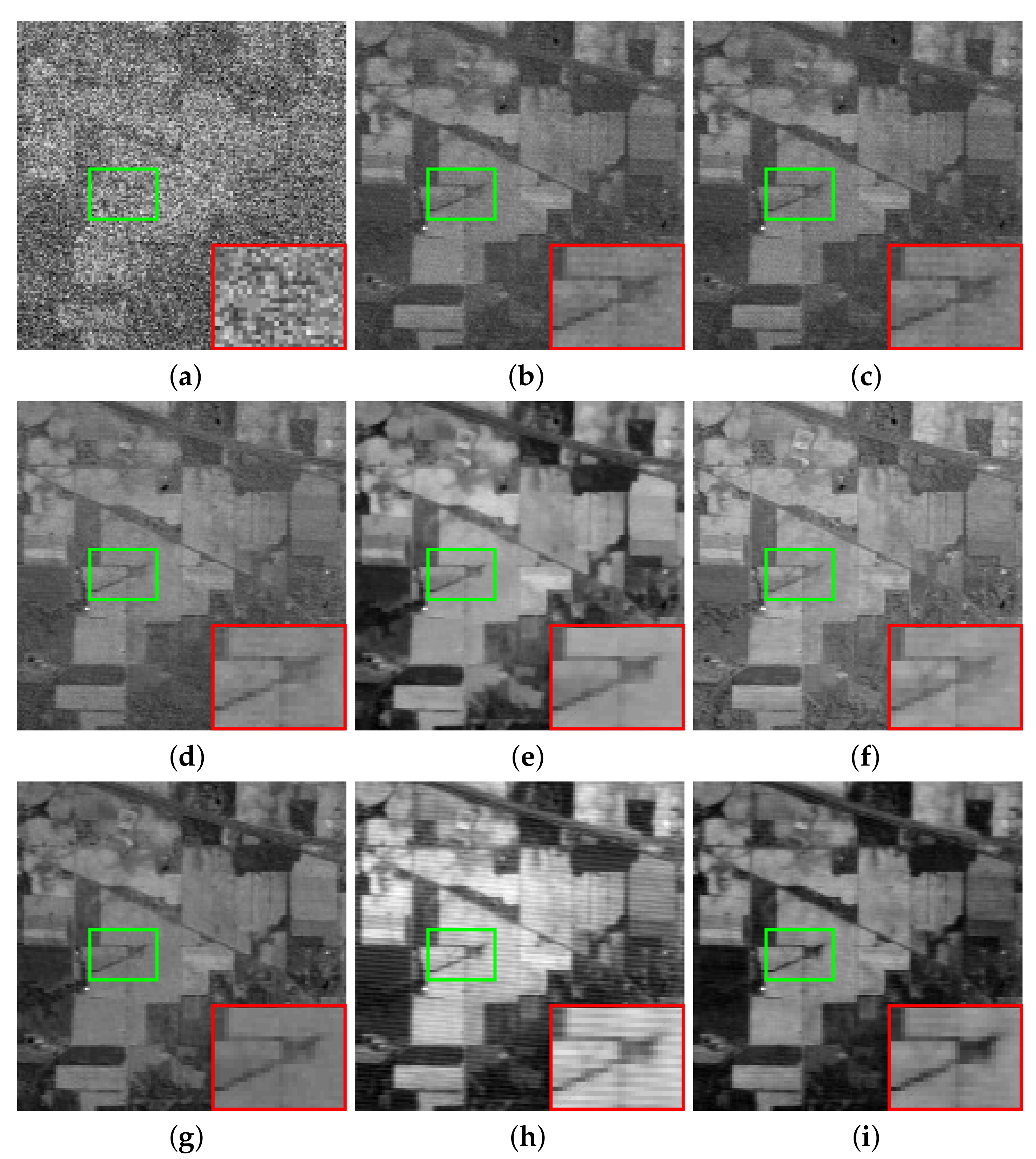
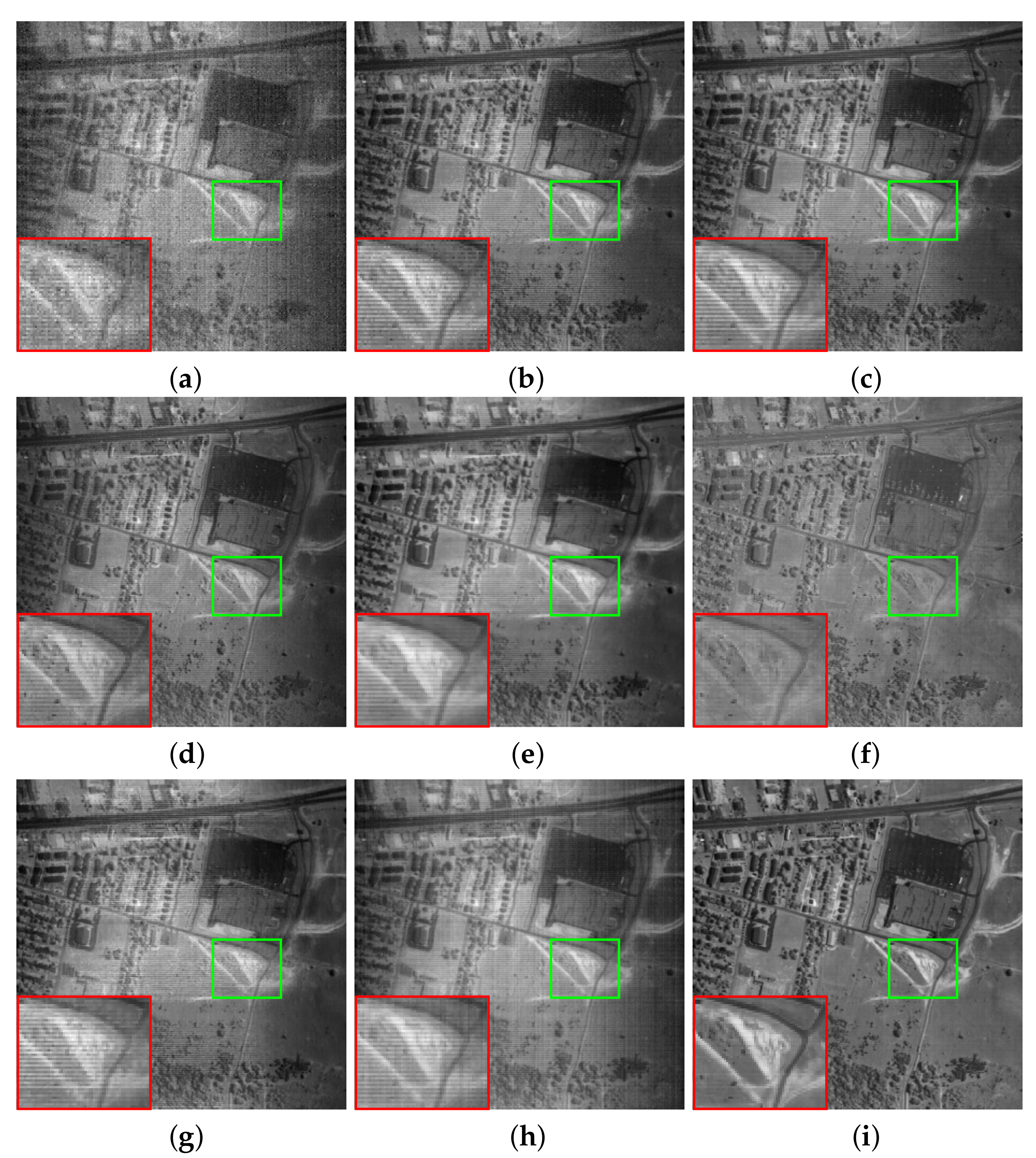
We show some bands of the Pavia denoised results to reflect the visual advantages of our model. We selected band 65 under the noise case 3 and band 60 under the noise case 8 for image display, which are shown in Figure 3. From Figure 3, one can see that, due to noise pollution, the quality of the original HSIs has degraded to a large extent, as shown in Figure 3a. Dealt with by different denoising methods, the image quality has been improved to a certain extent. Obviously, the LRTA, BM4D, LRMR methods do not have a satisfying effect on noise removal. LRMR is better than LRTA and BM4D. However, the image still has a lot of visible noise. LRTDTV smoothes the image and blurs the details. L1HyMixDe and LRTDGS are not ideal for edge texture processing. In Figure 3f, the loss of textural information is obvious. The denoising effect of 3DTNN and our model is relatively good, but in terms of the restoration of the bright part, our model is clearly better than 3DTNN. In Figure 4, the original image is added with Gaussian noise, sparse noise, dead line noise, and stripe noise. Dealt with by different denoising methods, the LRTA, BM4D, LRMR methods cannot achieve the efficient denoising results. LRTDTV still has the problem that it loses the image details and smoothes the image. L1HyMixDe, LRTDGS and 3DTNN are still insufficient in removing stripe noise. As a result, the denoising results of our method are better than other denoised methods, which are chosen for visual comparison.

(B) Quantitative Comparison

We choose MPSNR over all bands, MSSIM over all bands, and SAM to objectively describe and compare image quality. It is clear that we need to ensure that MPSNR and MSSIM are large enough and that SAM is small enough, which means a superior denoising performance.

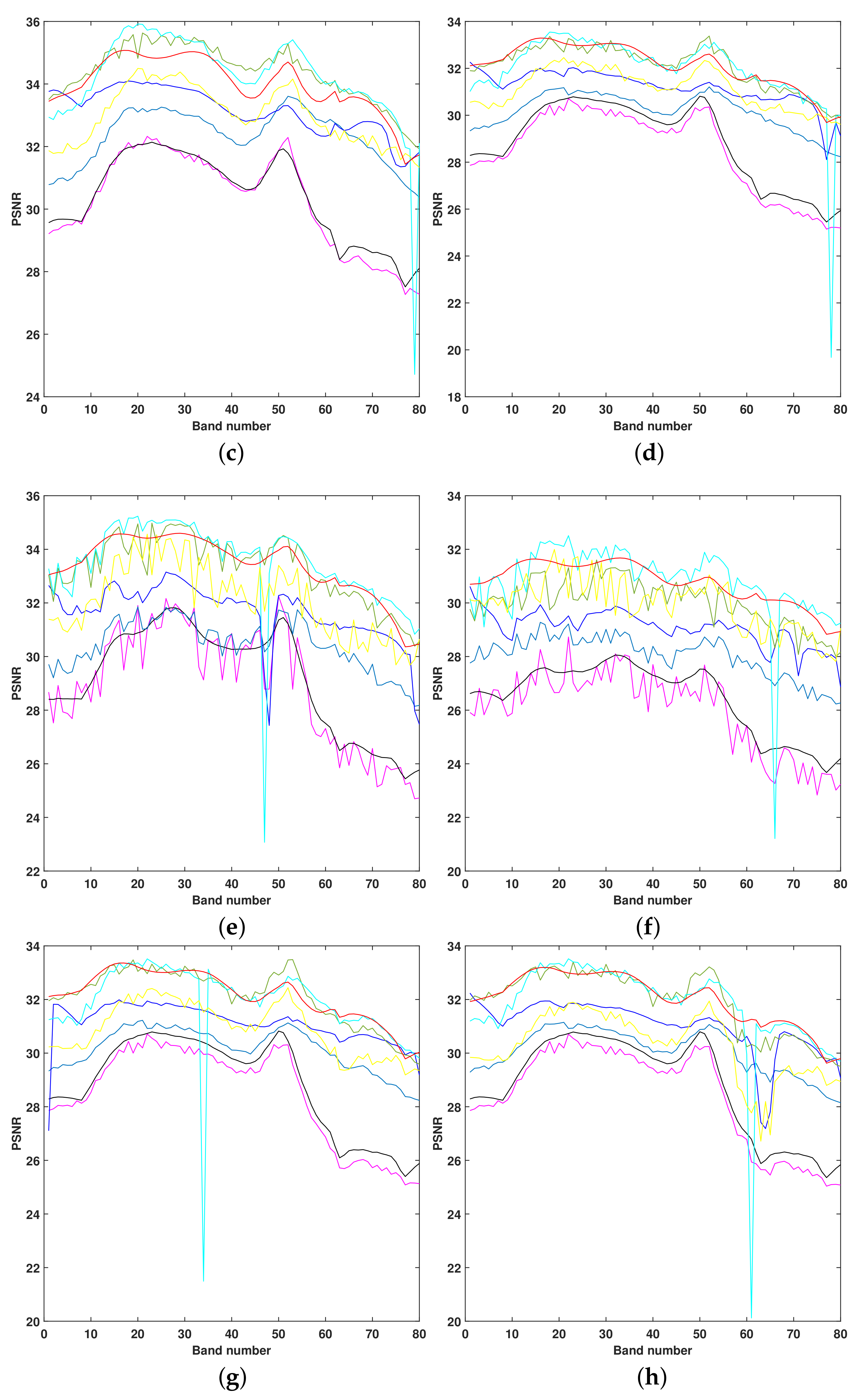
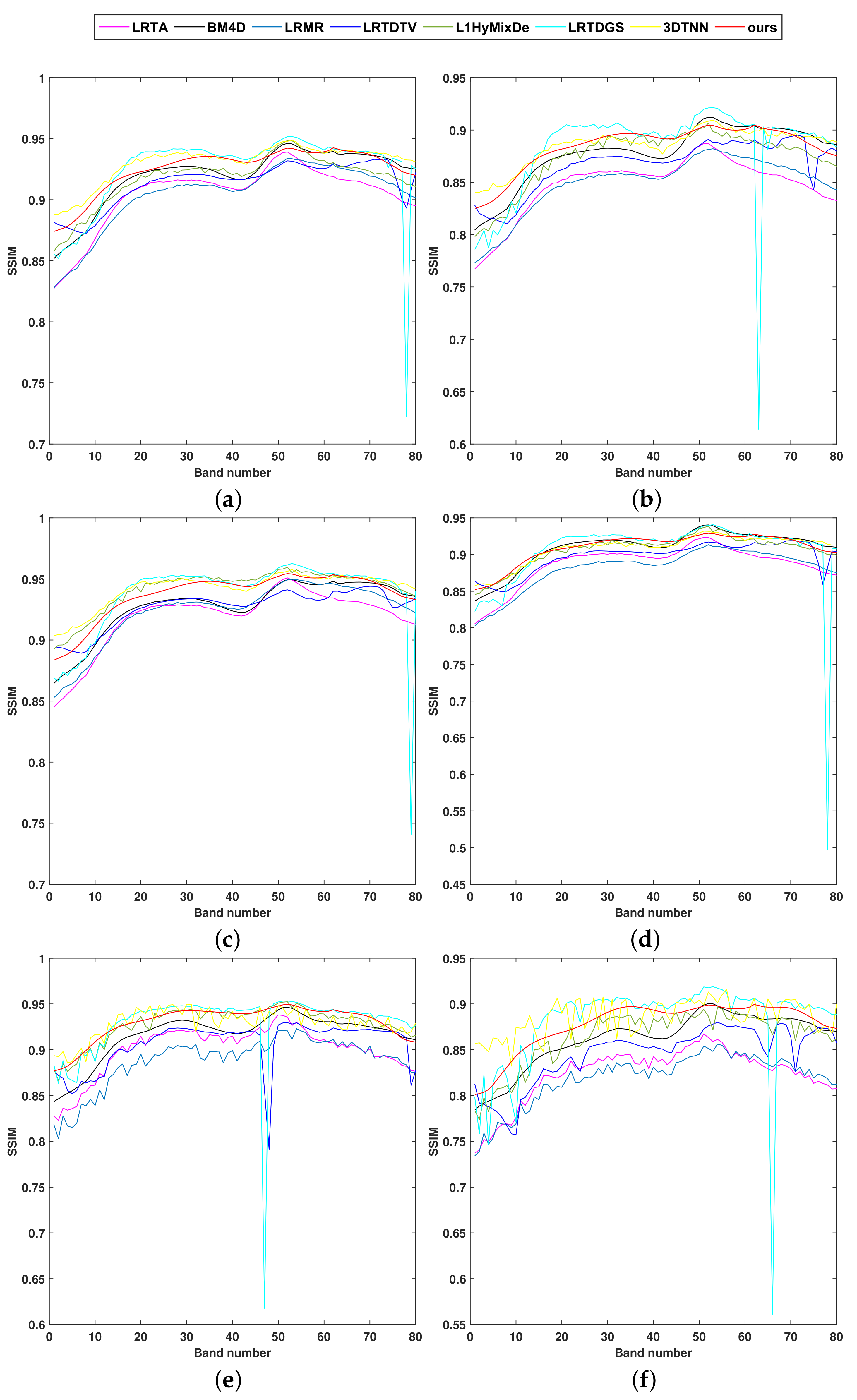
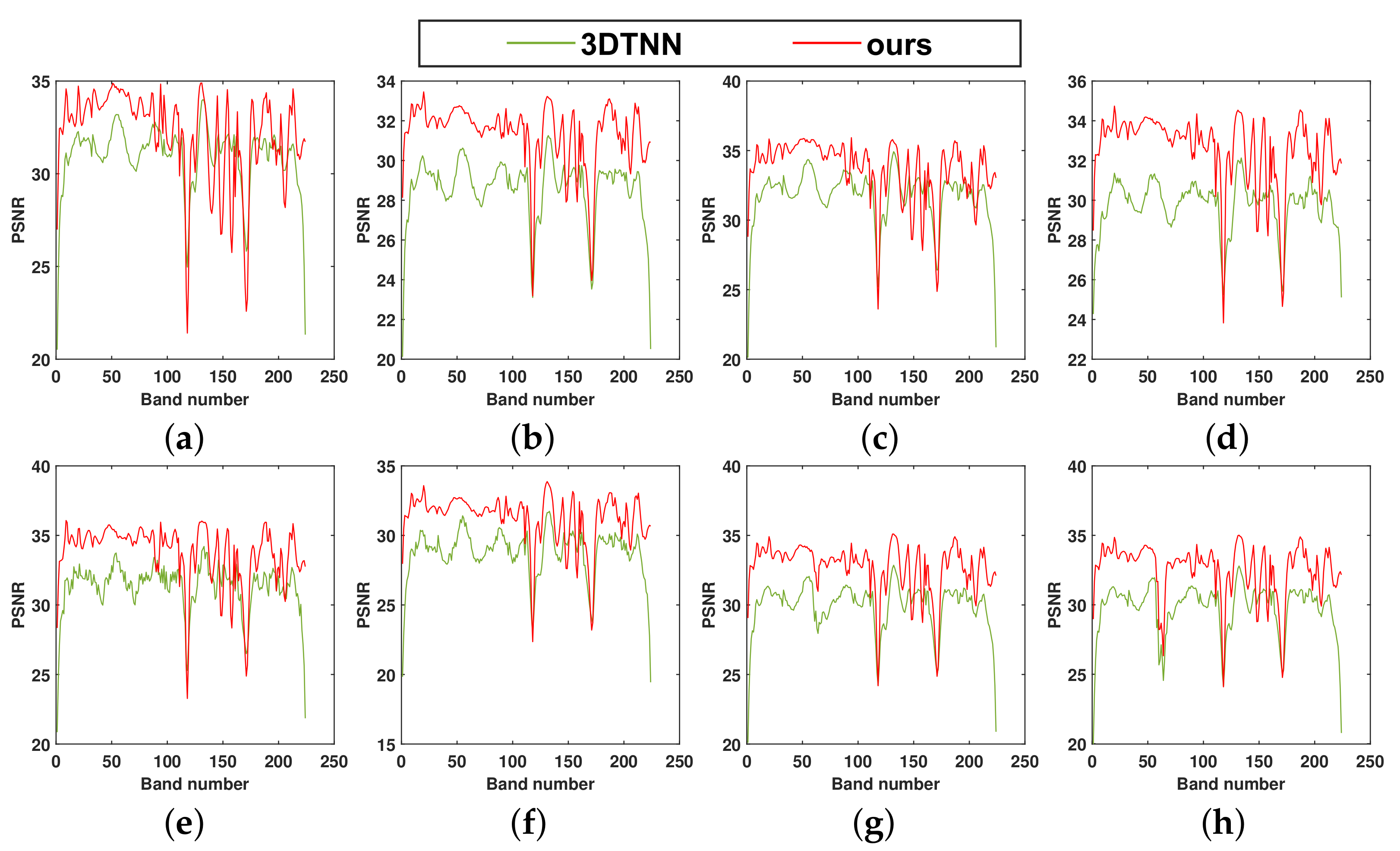
Under the different eight noise cases,

Table 3. The value of quantitative indices in the dataset-1.

Noise Case	Level	Evaluation Index	LRTA	BM4D	LRMR	LRTDT	L1HyMixDe	LRTDGS	3DTNN	Our
Case 1		MPSNR	29.4396	29.7014	31.2593	32.2970	32.9077	33.2535	32.1996	32.9243
	G = 0.1	MSSIM	0.9048	0.9203	0.9045	0.9138	0.9177	0.9253	0.9307	0.9256
	P = 0.2	SAM	6.8049	5.8404	6.8244	4.9305	4.4064	4.3546	3.4856	3.7368
Case 2		MPSNR	27.0258	27.4204	29.0133	30.1107	30.6235	30.9044	29.8947	30.9274
	G = 0.15;	MSSIM	0.8480	0.8787	0.8494	0.8669	0.8745	0.8833	0.8854	0.8857
	P = 0.2	SAM	7.8247	6.6710	7.6899	5.8480	4.9587	5.4792	4.2935	4.4098
Case 3		MPSNR	30.2658	30.3936	32.3389	33.1557	34.3770	34.2453	32.9942	33.9806
	G = 0.1	MSSIM	0.9190	0.9281	0.9237	0.9267	0.9421	0.9374	0.9423	0.9477
	P = 0.1	SAM	6.4482	5.5052	6.4019	4.6077	3.5472	4.0836	3.1475	3.6220
Case 4		MPSNR	28.4836	28.8640	30.1731	31.1878	32.1109	31.9825	31.1434	32.1440
	G = 0.1	MSSIM	0.8868	0.9098	0.8814	0.8972	0.9068	0.9057	0.9088	0.9099
	P = 0.3	SAM	7.2045	6.2362	7.2500	5.3489	4.7865	5.4171	4.3108	4.1209
Case 5		MPSNR	28.9336	29.1991	30.4432	31.6456	33.2988	33.5211	32.1036	33.8946
	G = (0.05,0.15)	MSSIM	0.9003	0.9161	0.8880	0.9062	0.9283	0.9293	0.9293	0.9302
	P = 0.2	SAM	7.1954	6.0548	7.1967	5.2504	4.2118	4.2629	3.6644	3.8739
Case 6		MPSNR	26.0073	26.4507	28.0358	29.0656	30.0129	30.8340	29.9707	30.7688
	G = (0.1,0.2)	MSSIM	0.8239	0.8621	0.8188	0.8452	0.8640	0.8808	0.8859	0.8777
	P = 0.2	SAM	8.3887	6.9711	8.1535	6.4062	5.5859	5.5074	4.5080	4.2183
Case 7	G = 0.1	MPSNR	28.4375	28.8168	30.1479	31.1278	32.1303	31.9213	30.9232	32.1686
	P = 0.3	MSSIM	0.8863	0.9095	0.8812	0.8951	0.9108	0.9079	0.9123	0.9167
	+deadline	SAM	7.2212	6.2393	7.2828	5.3694	6.6968	6.7940	5.2777	4.1205
Case 8	G = 0.1 P = 0.3	MPSNR	28.3902	28.7718	30.0586	31.0073	31.9432	31.8225	30.2764	32.0232
	+deadline	MSSIM	0.8852	0.9088	0.8798	0.8939	0.9075	0.9068	0.9027	0.9063
	+stripe	SAM	7.2192	6.2496	7.3609	5.6445	6.9130	7.1390	5.7186	4.3586

The best is in bold.

shows the values of indices of eight denoising methods for quantitative assessment in dataset-1. We overstrike the best values of each index to emphasize them. It can be seen that, on almost all indices, the proposed model has a better performance than the other comparable methods. Under strong noise, this phenomenon is particularly noticeable. Taking the MPSNR in case 3 as an example, compared with 3DTNN, our model is 1 dB higher than 3DTNN. In case 5, this value is as high as 1.8 dB. The PSNR and the SSIM for all denoised bands are listed in Figure Figure 5 and Figure 6. As a result, compared to other methods, the proposed model has a better performance in PSNR and SSIM values in most denoised bands.

Figure 7 shows the spectral curves at pixel (30, 30) denoised by all denoising methods in noise case 5. It is clear that, due to the noise, spectral curves fluctuate violently, and then the fluctuation amplitude is depressed after denoising by various methods. What is more, it is obvious that, in our denoised HSI, the spectral curves have fewer spectral distortions. Thus, in all the chosen methods, from the perspective of removing mixed noise, the proposed model obtains excellent denoising results.

4.1.2. USGS Indian Pines Dataset

Based on the result in dataset-1, we compare the denoising performance of our method and the method we want to improve under eight noise conditions in dataset-2. Then, the visual comparison of the denoising effect of 3DTNN and the proposed model under the third and sixth noise conditions are shown in Figure 8 and Figure 9. From the figure, we can see that our model is better than 3DTNN for the processing of details.

We also compare the quantitative indices to appraise the denoising effect in the dataset-2. The indices for quantitative assessment are listed in

Table 4. The value of quantitative indices in the dataset-2.

Noise Case	Level	MPSNR	3DTNN MSSIM	SAM	MPSNR	Our MSSIM	SAM
Case 1	G = 0.1	30.9073	0.9050	2.7583	32.1435	0.8964	2.7254
	P = 0.2
Case 2	G = 0.15	28.5602	0.8697	3.5259	31.3247	0.9013	2.5945
	P = 0.2
Case 3	G = 0.1	31.6945	0.9185	2.5888	33.6358	0.9170	2.2334
	P = 0.1
Case 4	G = 0.1	29.7186	0.8931	2.8884	32.5633	0.9080	2.3556
	P = 0.3
Case 5	G = (0.05,0.15)	31.2729	0.9089	2.6462	33.7245	0.9329	2.1341
	P = 0.2
Case 6	G = (0.1,0.2)	28.7189	0.8699	3.5476	31.2484	0.9076	2.6554
	P = 0.2
Case 7	G = 0.1 P = 0.3	29.9070	0.8747	3.1159	32.7050	0.9274	2.2178
	+deadline
Case 8	G = 0.1 P = 0.3	29.7521	0.8653	3.2478	32.5152	0.9256	2.3006
	+deadline +stripe

The best is in bold.

. The boldface means the best values. For almost all indices, our model is more effective at denoising than 3DTNN. Under strong noise, this phenomenon is particularly noticeable. Subsequently, the values of the PSNR and the SSIM are listed in Figure 10 and Figure 11. It is clear that our model has obvious advantages under higher noise intensity. For all the denoising methods we used in noise case 4, the spectral curves at pixel (100,30) are shown in Figure 12. One can find that the HSI dealt by our model has fewer spectral distortions, compared with 3DTNN.

4.2. Experiments on Real Datasets

We chose the AVIRIS Indian Pines dataset [48] (abbreviated as dataset-3) and the HYDICE Urban dataset [49] (abbreviated as dataset-4) as the real datasets to design and perform experiments, which are shown in Figure 13. Dataset-3 was collected by the Airborne Visible Infrared Imaging Spectrometer (AVIRIS) over the Indian Pines in Northwestern Indiana in 1992. Its size was $145\times 145\times 220$. Dataset-4 was acquired by the Hydice sensor, the size of which was $307\times 307\times 210$.

4.2.1. AVIRIS Indian Pines Dataset

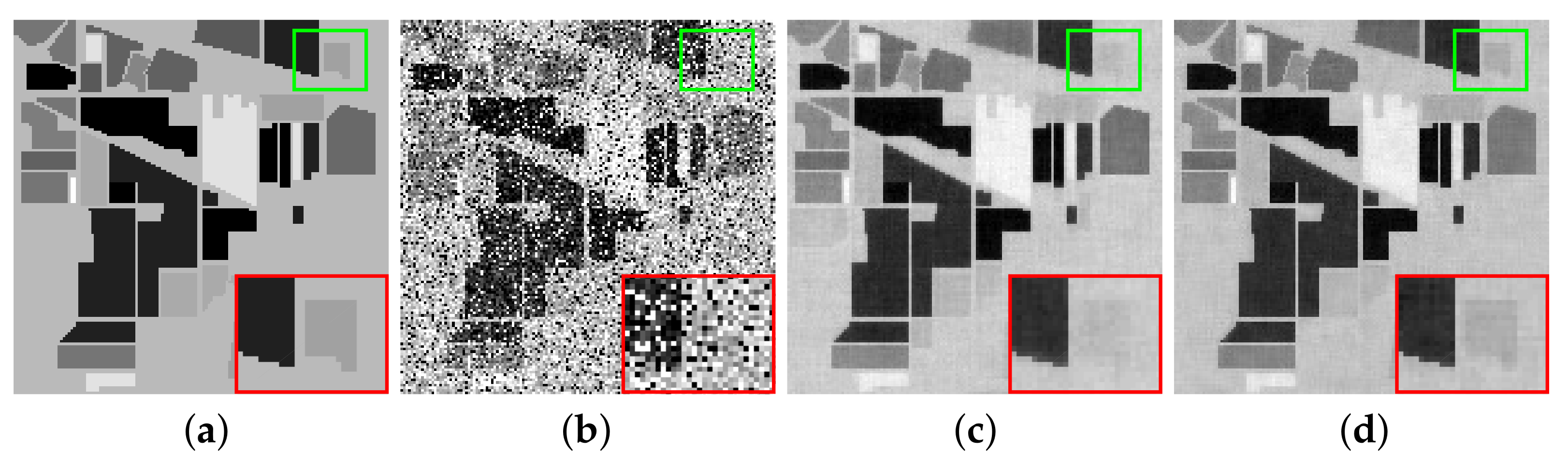
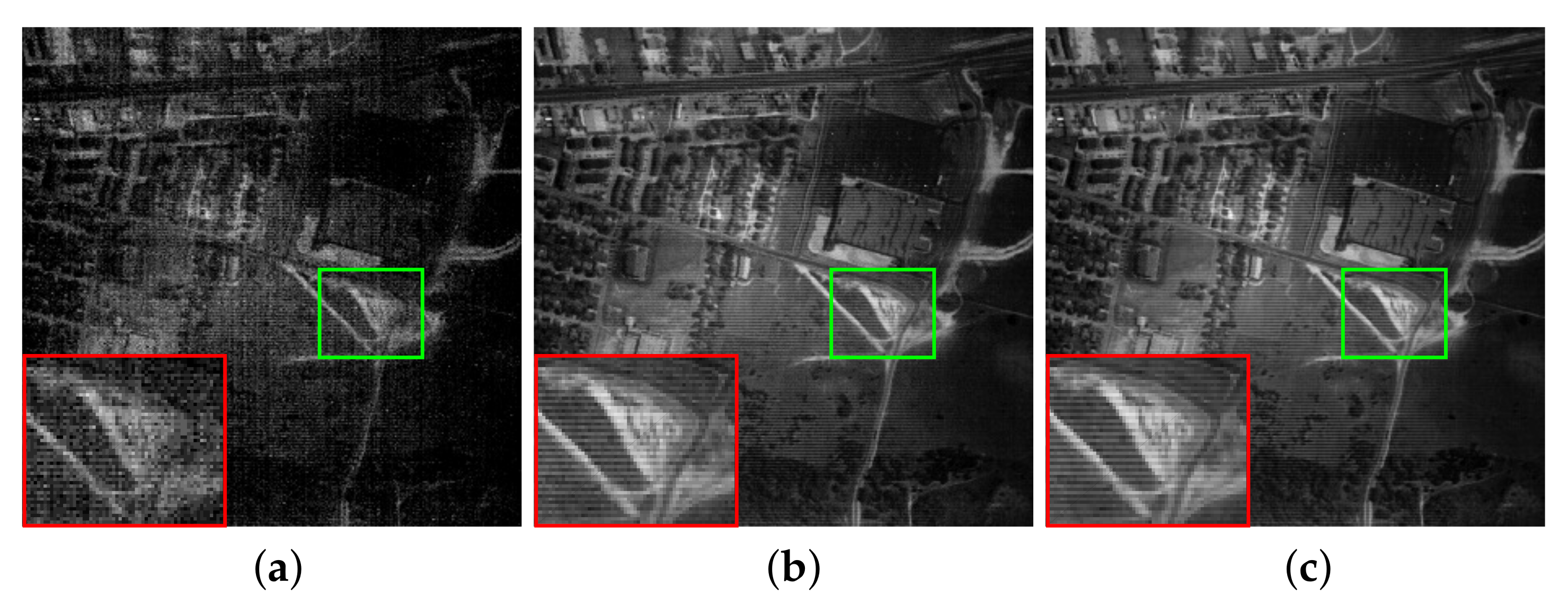
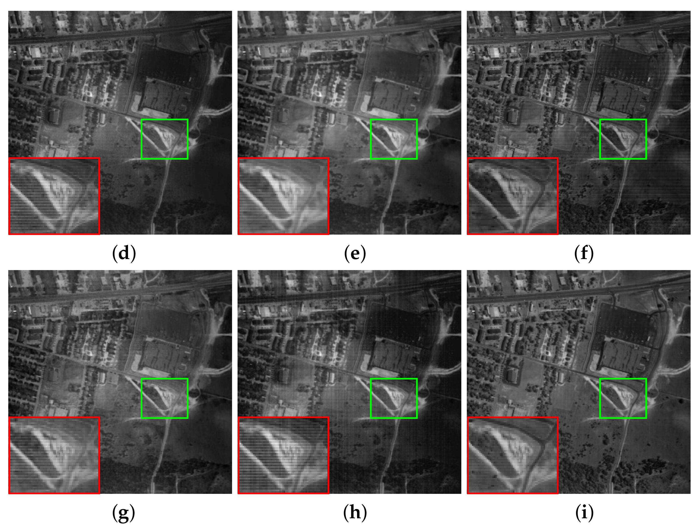
To display the effect of various denoising methods, we chose bands 106 and 163 of the denoised images to show in Figure 14 and Figure 15. The original image has been completely polluted by mixed noise, which is shown in Figure 14a and Figure 15a. After denoising, the denoising effect of LRTA, BM4D, and LRMR was incomplete, and there were still many visible noises. LRTDTV, L1HyMixDe, LRTDGS and 3DTNN could mainly remove the mixed noise. However, LRTDTV, L1HyMixDe and LRTDGS made the image too smooth, which led to the details, shown in red boxes, being seriously degraded. 3DTNN did not have a good effect on fringe noise. As a result, our model has the best performance in maintaining complete texture information, at the same time, depressing the mixed noise.

4.2.2. HYDICE Urban Dataset

Similar to dataset-3, we also chose two typical noise bands of dataset-4 to display the effect of various denoising methods. Bands 104 and 109 of the denoised images are shown in Figure 16 and Figure 17. As shown in Figure 16 and Figure 17, all methods can remove most of the mixed noises and restore the image structure. However, the images denoised by LRTA, BM4D and LRMR still preserve some part of the noise. LRTDTV and L1HyMixDe oversmooth the image. LRTDGS and 3DTNN have limitations on fringe noise. Compared with these methods, our method performs the best at removing noise while at the same time preserving details.

4.3. Ablation Experiment

To investigate the necessity of exploring the low-rankness of three modes in F-MTNN, we conducted several ablation studies. We took dataset-1, noise case 3 as an example. By setting $\omega (\omega =({\omega }_1,{\omega }_2,{\omega }_3))$, we made the model explore low-rank information only along spatial or spectral dimensions, compared with the result of F-3MTNN. We show the values of PSNR and SSIM in

Table 5. The ablation experiment of F-3MTNN.

Spatial Information	Spectral Information	PSNR	SSIM
✓		21.7398	0.3938
	✓	25.8850	0.7504
✓	✓	30.9274	0.8857

The best is in bold.

. The proposed model, which explores the low-rankness of both spatial and spectral dimensions at the same time, can achieve the most efficient results.

5. Discussion

5.1. Parameter Analysis

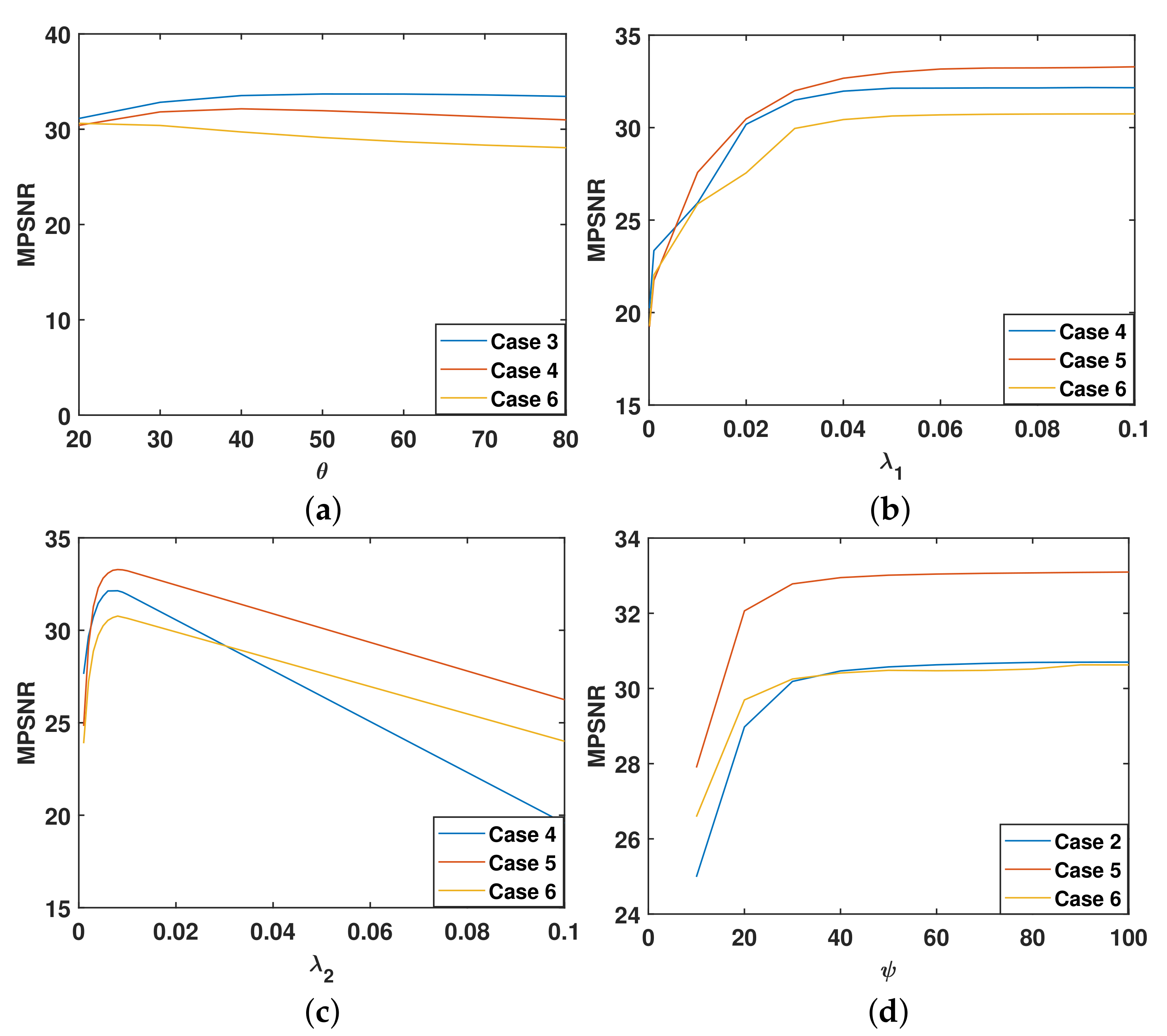
We develop a sensitivity analysis of the parameters used in our method including the weight $\omega$ ($\omega =({\omega }_1,{\omega }_2,{\omega }_3)$), the regularization parameters ${\lambda }_1$, ${\lambda }_2$, and the threshold parameter $\tau =\omega /\mu$. For each parameter, data in three cases of the experiment on dataset-1 are randomly selected for display.

The weight $\omega$ is set as $(1,1,\theta )/(2+\theta )$, which controls the proportion of each mode correlation of HSI, where $\theta$ is a balance parameter to control $\omega$. We can find the appropriate weight $\omega$ easily. Figure 18a presents the sensitivity analysis of $\theta$. According to Figure 18a, when $\theta >35$, the PSNR value in our method is nearly stable.

The regularization parameters ${\lambda }_1,{\lambda }_2$ control the weight of Gaussian noise and sparse noise respectively. The sensitivity analysis of ${\lambda }_1,{\lambda }_2$ is shown in Figure 18b,c. For the ${\lambda }_1$, when ${\lambda }_1>0.04$, the PSNR value in our method is nearly stable. However, as observed, it is sensitive to ${\lambda }_2$. It especially achieves the highest PSNR value when ${\lambda }_2=0.007$.

We choose the threshold parameter $\tau$ as $\psi \times (1,1,1)$. Figure 18d shows the sensitivity analysis of $\psi$. We find that, when $\psi >40$, the MPSNR values maintain a high level and, when $\psi <40$, the recovery effect is not satisfactory. The main reason is that noise occupies a larger proportion of small singular values, and too little shrinkage parameter will result in incomplete noise removal.

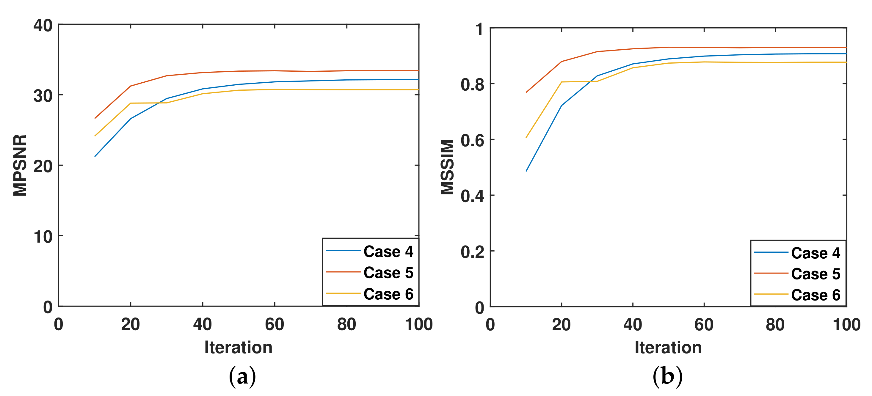
5.2. Convergence Analysis

The change of MPSNR and MSSIM values as the number of iterations increases is shown in Figure 19. From the figure, we can observe that, after several iterations, the values of these two indicators become stable by degrees, which means our algorithm is convergent.

5.3. Running Time

The running time is shown in

Table 6. The running time (in seconds) of the different methods in the real HSI dataset experiments.

HSI Data	LRTA	BM4D	LRMR	LRTDTV	L1HyMixDe	LRTDGS	3DTNN	Our
AVIRIS Indian Pines	35	261	412	131	4	123	87	1259
HYDICE Urban	143	4076	6132	960	7	811	1503	6602

, which measures the efficiency of all denoising methods used in this paper. The proposed model focuses on the improvement of accuracy. At the same time, due to the redundancy of the framelet, the running time will inevitably increase. However, it can be improved in terms of computing time. For each iteration, the parallel processing can be used in the calculations of three modes, which will greatly improve computational efficiency. This is also an improvement that needs to be considered in future work.

6. Conclusions

In this paper, we first use the framelet to define the framelet-based tensor fibered rank, which is more conducive to the accurate exploration of the global low-rankness of tensors. Furthermore, we develop the F-3MTNN as its convex approximation, which means that the information of each dimension of HSI is fully explored. Then, F-3DTNN is applied in a new denoising model. Finally, to compute this convex model with guaranteed convergence, we create a fast algorithm based on ADMM. By comparing with the latest competing methods, including LRTA, BM4D, LRMR, LRTDTV, L1HyMixDe, LRTDGS and 3DTNN, our model has the ability to remove mixed noise effectively and to retain necessary details.

The method we proposed provides a more accurate characterization of the low-rankness of tensors; however, long CPU time leads to poor applicability in applications. In follow-up research, we will adopt parallel computing and other forms to improve the universality of model applications. In addition, the model can also be applied to data processing tasks such as image deblurring, image compression and super-resolution reconstruction.

References

- Bioucas-Dias, J.M.; Plaza, A.; Dobigeon, N.; Parente, M.; Du, Q.; Gader, P.; Chanussot, J. Hyperspectral unmixing overview: Geometrical, statistical, and sparse regression-based approaches. IEEE J. Sel. Top. Appl. Earth Observ. Remote Sens. 2012, 5, 354–379. [Google Scholar] [CrossRef] [Green Version]
- Li, S.; Dian, R.; Fang, L.; Bioucas-Dias, J.M. Fusing hyperspectral and multispectral images via coupled sparse tensor factorization. IEEE Trans. Image Process. 2018, 27, 4118–4130. [Google Scholar] [CrossRef] [PubMed]
- Gao, L.; Yao, D.; Li, Q.; Zhuang, L.; Zhang, B.; Bioucas-Dias, J.M. A new low-rank representation based hyperspectral image denoising method for mineral mapping. Remote Sens. 2017, 9, 1145. [Google Scholar] [CrossRef] [Green Version]
- Zeng, H.; Xie, X.; Ning, J. Hyperspectral image denoising via global spatial-spectral total variation regularized nonconvex local low-rank tensor approximation. Signal Process. 2021, 178, 107805. [Google Scholar] [CrossRef]
- Zheng, Y.; Huang, T.; Zhao, X.; Jiang, T.; Ji, T. Mixed noise removal in hyperspectral image via low-fibered-rank regularization. IEEE Trans. Geosci. Remote Sens. 2019, 58, 734–749. [Google Scholar] [CrossRef]
- Zeng, H.; Xie, X.; Cui, H.; Yin, H.; Ning, J. Hyperspectral Image Restoration via Global L 1-2 Spatial–Spectral Total Variation Regularized Local Low-Rank Tensor Recovery. IEEE Trans. Geosci. Remote Sens. 2020, 59, 3309–3325. [Google Scholar] [CrossRef]
- Ma, A.; Zhong, Y.; Zhao, B.; Jiao, H.; Zhang, L. Semisupervised subspace-based dna encoding and matching classifier for hyperspectral remote sensing imagery. IEEE Trans. Geosci. Remote Sens. 2016, 54, 4402–4418. [Google Scholar] [CrossRef]
- Yang, S.; Shi, Z. Hyperspectral image target detection improvement based on total variation. IEEE Trans. Image Process. 2016, 25, 2249–2258. [Google Scholar] [CrossRef] [PubMed]
- Zhang, H.; Zhai, H.; Zhang, L.; Li, P. Spectral–spatial sparse subspace clustering for hyperspectral remote sensing images. IEEE Trans. Geosci. Remote Sens. 2016, 54, 3672–3684. [Google Scholar] [CrossRef]
- Ji, H.; Liu, C.Q.; Shen, Z.W.; Xu, Y.H. Robust video denoising using low rank matrix completion. In Proceedings of the 23rd IEEE Conference on Computer Vision and Pattern Recognition, CVPR 2010, San Francisco, CA, USA, 13–18 June 2010. [Google Scholar]
- Ji, H.; Huang, S.; Shen, Z.; Xu, Y. Robust video restoration by joint sparse and low rank matrix approximation. SIAM J. Imaging Sci. 2011, 4, 1122–1142. [Google Scholar] [CrossRef]
- Maggioni, M.; Katkovnik, V.; Egiazarian, K.; Foi, A. Nonlocal transform-domain filter for volumetric data denoising and reconstruction. IEEE Trans. Image Process. 2012, 22, 119–133. [Google Scholar] [CrossRef]
- Zhang, H.; He, W.; Zhang, L.; Shen, H.; Yuan, Q. Hyperspectral image restoration using low-rank matrix recovery. IEEE Trans. Geosci. Remote Sensing 2014, 52, 4729–4743. [Google Scholar] [CrossRef]
- He, W.; Zhang, H.; Zhang, L.; Shen, H. Hyperspectral image denoising via noise-adjusted iterative low-rank matrix approximation. IEEE J. Sel. Top. Appl. Earth Observ. Remote Sens. 2015, 8, 1–12. [Google Scholar] [CrossRef]
- Zheng, Y.; Huang, T.; Ji, T.; Zhao, X.; Jiang, T.; Ma, T. Low-rank tensor completion via smooth matrix factorization. Appl. Math. Model. 2019, 70, 677–695. [Google Scholar] [CrossRef]
- Cao, X.; Zhao, Q.; Meng, D.; Chen, Y.; Xu, Z. Robust low-rank matrix factorization under general mixture noise distributions. IEEE Trans. Image Process. 2016, 25, 4677–4690. [Google Scholar] [CrossRef] [PubMed] [Green Version]
- Wang, J.; Huang, T.; Ma, T.; Zhao, X.; Chen, Y. A sheared low-rank model for oblique stripe removal. Appl. Math. Comput. 2019, 360, 167–180. [Google Scholar] [CrossRef]
- Zeng, H.; Xie, X.; Cui, H.; Zhao, Y.; Ning, J. Hyperspectral image restoration via cnn denoiser prior regularized low-rank tensor recovery. Comput. Vis. Image Underst. 2020, 197, 103004. [Google Scholar] [CrossRef]
- Zhuang, L.; Bioucas-Dias, J.M. Fast hyperspectral image denoising and inpainting based on low-rank and sparse representations. IEEE J. Sel. Top. Appl. Earth Observ. Remote Sens. 2018, 11, 730–742. [Google Scholar] [CrossRef]
- Zhuang, L.; Fu, X.; Ng, M.K.; Bioucas-Dias, J.M. Hyperspectral image denoising based on global and nonlocal low-rank factorizations. IEEE Trans. Geosci. Remote Sens. 2021, in press. [Google Scholar]
- Jiang, T.; Zhuang, L.; Huang, T.; Zhao, X.; Bioucas-Dias, J.M. Adaptive hyperspectral mixed noise removal. IEEE Trans. Geosci. Remote Sens. 2021, in press. [Google Scholar]
- Chen, Y.; Cao, X.; Zhao, Q.; Meng, D.; Xu, Z. Denoising hyperspectral image with non-iid noise structure. IEEE Trans. Cybern. 2017, 48, 1054–1066. [Google Scholar] [CrossRef] [PubMed] [Green Version]
- Acar, E.; Dunlavy, D.M.; Kolda, T.G.; Mørup, M. Scalable tensor factorizations for incomplete data. Chemometrics Intell. Lab. Syst. 2011, 106, 41–56. [Google Scholar] [CrossRef] [Green Version]
- Tichavsky, P.; Phan, A.; Cichocki, A. Numerical cp decomposition of some difficult tensors. J. Comput. Appl. Math. 2017, 317, 362–370. [Google Scholar] [CrossRef] [Green Version]
- Li, Y.; Shang, K.; Huang, Z. Low tucker rank tensor recovery via admm based on exact and inexact iteratively reweighted algorithms. J. Comput. Appl. Math. 2018, 331, 64–81. [Google Scholar] [CrossRef]
- Li, X.; Ng, M.K.; Cong, G.; Ye, Y.; Wu, Q. Mr-ntd: Manifold regularization nonnegative tucker decomposition for tensor data dimension reduction and representation. IEEE Trans. Neural Netw. Learn. Syst. 2016, 28, 1787–1800. [Google Scholar] [CrossRef] [PubMed]
- Hillar, C.J.; Lim, L. Most tensor problems are np-hard. J. ACM 2013, 60, 1–39. [Google Scholar] [CrossRef]
- Jiang, T.; Ng, M.K.; Zhao, X.; Huang, T. Framelet representation of tensor nuclear norm for third-order tensor completion. IEEE Trans. Image Process. 2020, 29, 7233–7244. [Google Scholar] [CrossRef]
- Braman, K. Third-order tensors as linear operators on a space of matrices. Linear Alg. Appl. 2010, 433, 1241–1253. [Google Scholar] [CrossRef] [Green Version]
- Kilmer, M.E.; Martin, C.D. Factorization strategies for third-order tensors—sciencedirect. Linear Alg. Appl. 2011, 435, 641–658. [Google Scholar] [CrossRef] [Green Version]
- Kernfeld, E.; Kilmer, M.; Aeron, S. Tensor–tensor products with invertible linear transforms. Linear Alg. Appl. 2015, 485, 545–570. [Google Scholar] [CrossRef]
- Liu, Y.; Zhao, X.; Zheng, Y.; Ma, T.; Zhang, H. Hyperspectral image restoration by tensor fibered rank constrained optimization and plug-and-play regularization. IEEE Trans. Geosci. Remote Sens. 2021, in press. [Google Scholar]
- Kilmer, M.E.; Braman, K.; Hao, N.; Hoover, R.C. Third-order tensors as operators on matrices: A theoretical and computational framework with applications in imaging. SIAM J. Matrix Anal. Appl. 2013, 34, 148–172. [Google Scholar] [CrossRef] [Green Version]
- Song, G.; Ng, M.K.; Zhang, X. Robust tensor completion using transformed tensor svd. arXiv 2019, arXiv:1907.01113. [Google Scholar]
- Cai, J.; Chan, R.; Shen, Z. A framelet-based image inpainting algorithm. Appl. Comput. Harmon. Anal. 2008, 24, 131–149. [Google Scholar] [CrossRef] [Green Version]
- Boyd, S.; Parikh, N.; Chu, E.; Peleato, B.; Eckstein, J. Distributed optimization and statistical learning via the alternating direction method of multipliers. Found. Trends Mach. Learn. 2010, 3, 1–122. [Google Scholar] [CrossRef]
- Jiang, T.; Huang, T.; Zhao, X.; Ji, T.; Deng, L. Matrix factorization for low-rank tensor completion using framelet prior. Inf. Sci. 2018, 436, 403–417. [Google Scholar] [CrossRef]
- Zeng, H.; Xie, X.; Kong, W.; Cui, S.; Ning, J. Hyperspectral image denoising via combined non-local self-similarity and local low-rank regularization. IEEE Access 2020, 8, 50190–50208. [Google Scholar] [CrossRef]
- Ron, A.; Shen, Z. Affine systems inl2(rd): The analysis of the analysis operator. J. Funct. Anal. 1997, 148, 408–447. [Google Scholar] [CrossRef] [Green Version]
- Cai, J.; Candès, E.J.; Shen, Z. A singular value thresholding algorithm for matrix completion. SIAM J. Optim. 2010, 20, 1956–1982. [Google Scholar] [CrossRef]
- Lin, Z.; Chen, M.; Ma, Y. The augmented lagrange multiplier method for exact recovery of corrupted low-rank matrices. arXiv 2010, arXiv:1009.5055. [Google Scholar]
- Renard, N.; Bourennane, S.; Blanc-Talon, J. Denoising and dimensionality reduction using multilinear tools for hyperspectral images. IEEE Geosci. Remote Sens. Lett. 2008, 5, 138–142. [Google Scholar] [CrossRef]
- Wang, Y.; Peng, J.; Zhao, Q.; Leung, Y.; Zhao, X.; Meng, D. Hyperspectral image restoration via total variation regularized low-rank tensor decomposition. IEEE J. Sel. Top. Appl. Earth Observ. Remote Sens. 2017, 11, 1227–1243. [Google Scholar] [CrossRef] [Green Version]
- Chen, Y.; He, W.; Yokoya, N.; Huang, T. Hyperspectral image restoration using weighted group sparsity-regularized low-rank tensor decomposition. IEEE T. Cybern. 2020, 50, 3556–3570. [Google Scholar] [CrossRef] [PubMed]
- Zhuang, L.; Ng, M.K. Hyperspectral mixed noise removal by l1-norm based subspace representation. IEEE J. Sel. Top. Appl. Earth Observ. Remote Sens. 2020, 13, 1143–1157. [Google Scholar] [CrossRef]
- Pavia City Center Dataset. Available online: http://www.ehu.es/ccwintco/index.php/Hyperspectral_Remote_Sensing_Scenes (accessed on 8 March 2020).
- USGS Indian Pines Dataset. Available online: https://engineering.purdue.edu/%20biehl/MultiSpec/hyperspectral.html (accessed on 8 March 2020).
- AVIRIS Indian Pines Dataset. Available online: https://engineering.purdue.edu/%20biehl/MultiSpec/hyperspectral.html (accessed on 9 March 2020).
- HYDICE Urban Dataset. Available online: http://www.tec.army.mil/hypercube (accessed on 9 March 2020).
Figure 1.
The distribution of singular values on each frontal slice of the two different transformed tensors. (a) The first mode, (b) the second mode, (c) the third mode.
Figure 2.
(a) Pavia City Center dataset, (b) USGS Indian Pines dataset.
Figure 3.
(a) Original image, (b) noisy image, image denoised by (c) LRTA, (d) BM4D, (e) LRMR, (f) LRTDTV, (g) L1HyMixDe, (h) LRTDGS, (i) 3DTNN, (j) ours of band 65 in dataset-1, noise case 3.
Figure 4.
(a) Original image, (b) noisy image, image denoised by (c) LRTA, (d) BM4D, (e) LRMR, (f) LRTDTV, (g) L1HyMixDe, (h) LRTDGS, (i) 3DTNN, (j) ours of band 60 in dataset-1, noise case 8.
Figure 5.
The PSNR values of each band in dataset-1 after denoising by eight different methods under (a) case 1, (b) case 2, (c) case 3, (d) case 4, (e) case 5, (f) case 6, (g) case 7, (h) case 8.
Figure 6.
The SSIM values of each band in dataset-1 after denoising by eight different methods under (a) case 1, (b) case 2, (c) case 3, (d) case 4, (e) case 5, (f) case 6, (g) case 7, (h) case 8.
Figure 7.
The reflectance of pixel (30, 30) in (a) noisy dataset-1, dataset-1 denoised by (b) LRTA, (c) BM4D, (d) LRMR, (e) LRTDTV, (f) L1HyMixDe, (g) LRTDGS, (h) 3DTNN, (i) ours under noise case 4.
Figure 8.
(a) Original image, (b) noisy image, image denoised by (c) 3DTNN, (d) ours of band 26 in the dataset-2, noise case 2.
Figure 9.
(a) Original image, (b) noisy image, image denoised by (c) 3DTNN, (d) ours of band 4 in the dataset-2, noise case 5.
Figure 10.
The PSNR values of each band in the dataset-2 after denoising by 3DTNN and our model under (a) case 1, (b) case 2, (c) case 3, (d) case 4, (e) case 5, (f) case 6, (g) case 7, (h) case 8.
Figure 11.
The SSIM values of each band in the dataset-2 after denoising by 3DTNN and our model under (a) case 1, (b) case 2, (c) case 3, (d) case 4, (e) case 5, (f) case 6, (g) case 7, (h) case 8.
Figure 12.
The reflectance of pixel (100,30) in the dataset-2 denoised by (a) 3DTNN and (b) ours under noise case 3.
Figure 13.
(a) AVIRIS Indian Pines dataset, (b) HYDICE Urban dataset.
Figure 14.
(a) Original image, image denoised by (b) LRTA, (c) BM4D, (d) LRMR, (e) LRTDTV, (f) L1HyMixDe, (g) LRTDGS, (h) 3DTNN, (i) ours of band 106 in dataset-3.
Figure 15.
(a) Original image, image denoised by (b) LRTA, (c) BM4D, (d) LRMR, (e) LRTDTV, (f) L1HyMixDe, (g) LRTDGS, (h) 3DTNN, (i) ours of band 163 in dataset-3.
Figure 16.
(a) Original image, image denoised by (b) LRTA, (c) BM4D, (d) LRMR, (e) LRTDTV, (f) L1HyMixDe, (g) LRTDGS, (h) 3DTNN, (i) ours of band 104 in dataset-4.
Figure 17.
(a) Original image, image denoised by (b) LRTA, (c) BM4D, (d) LRMR, (e) LRTDTV, (f) L1HyMixDe, (g) LRTDGS, (h) 3DTNN, (i) ours of band 109 in dataset-4.
Figure 18.
PSNR values concerning different values of (a) (controls ), (b) , (c) and (d) (controls ).
Figure 19.
The change of (a) MPSNR value, (b) MSSIM value with the iteration.