Article

Monitoring Coastline Changes of the Malay Islands Based on Google Earth Engine and Dense Time-Series Remote Sensing Images

1
School of Surveying and Land Information Engineering, Henan Polytechnic University, Jiaozuo 454000, China
2
State Key Laboratory of Resources and Environmental Information System, Institute of Geographic Sciences and Natural Resources Research, Chinese Academy of Sciences, Beijing 100101, China
3
University of Chinese Academy of Sciences, Beijing 100049, China
*
Author to whom correspondence should be addressed.
Remote Sens. 2021, 13(19), 3842; https://0-doi-org.brum.beds.ac.uk/10.3390/rs13193842
Submission received: 13 August 2021 / Revised: 23 September 2021 / Accepted: 23 September 2021 / Published: 25 September 2021
(This article belongs to the Special Issue GIS and RS in Ocean, Island and Coastal Zone)

Abstract

:
The use of remote sensing to monitor coastlines with wide distributions and dynamic changes is significant for coastal environmental monitoring and resource management. However, most current remote sensing information extraction of coastlines is based on the instantaneous waterline, which is obtained by single-period imagery. The lack of a unified standard is not conducive to the dynamic change monitoring of a changeable coastline. The tidal range observation correction method can be used to correct coastline observation to a unified climax line, but it is difficult to apply on a large scale because of the distribution of observation sites. Therefore, we proposed a coastline extraction method based on the remote sensing big data platform Google Earth Engine and dense time-series remote sensing images. Through the instantaneous coastline probability calculation system, the coastline information could be extracted without the tidal range observation data to achieve a unified tide level standard. We took the Malay Islands as the experimental area and analyzed the consistency between the extraction results and the existing high-precision coastline thematic products of the same period to achieve authenticity verification. Our results showed that the coastline data deviated 10 m in proportion to a reach of 40% and deviated 50 m within a reach of 89%. The overall accuracy was kept within 100 m. In addition, we extracted 96 additional islands that have not been included in public data. The obtained multi-phase coastlines showed the spatial distribution of the changing hot regions of the Malay Islands’ coastline, which greatly supported our analysis of the reasons for the expansion and retreat of the coastline in this region. These research results showed that the big data platform and intensive time-series method have considerable potential in large-scale monitoring of coastline dynamic change and island reef change monitoring.

1. Introduction

As the coastline represents the boundary between the sea and the land, the delineation of the coastline position is important for coastal zone and island reef surveying and mapping [1]. The extraction and monitoring of coastlines are important for planning and protecting coastal areas, keeping residents safe, extracting islands and reefs, and developing navigation. Because the coastline is moved by processes such as waves, tidal currents, sea-level rise, subsidence, human activity, and many other factors [2], many uncertainties are inherent in the extraction and monitoring of coastlines. Therefore, the existing coastline monitoring methods have many limitations; for example, they are time-consuming and labor-intensive and have a limited monitoring range and long detection period. With the advent of remote sensing big data, remote sensing images have been widely used to extract and detect coastlines [3,4]. Now, researchers can use multiple types of satellites to obtain remote sensing data. The use of remote sensing data has changed the conventional data collection method, providing convenience for large-scale coastline research and providing an important guarantee for monitoring coastline temporal and spatial changes [5].
Until now, many scholars have used remote sensing images and adopted different methods to complete the extraction and analysis of the coastline. A method for semiautomatic coastline extraction based on TM (Thematic Mapper) and ETM+ (Enhanced Thematic Mapper) images was proposed, which uses a combination of the histogram threshold and frequency band ratio [6]. A semiautomatic extraction method proposed by Maglione et al. [7] is the maximum likelihood method, which is based on training points based on WorldView-2 images. Using edge detection operators to extract coastlines is another semiautomatic extraction method [8]. These semiautomatic extraction methods all realize the semiautomatic extraction of the coastline and achieve a certain level of accuracy, but the size of their application area is not sufficient and not suitable for large-scale promotion and use. Roger Sayre et al. proposed a method for the semiautomatic classification of images by manually selecting training points for representative waters and nonaquatic categories for the global coastline. This method has the advantages of a uniform method and large-scale application, but synthetic images are reduced to improve the feature detection of cloud interference, which is not included in tidal control, and the method ignores the existence of a high-water mark. Moreover, the vector result obtained represents only the water edge between the high-water mark and the low-water mark, that is, the waterline somewhere between the coastal zones [9]. In addition, Luijendijk et al. applied a coastline detection algorithm to cloud-free global annual composite images using more than 1.9 million historical Landsat images [10]. Zhang et al. also conducted extraction studies of coastlines, islands, and reefs based on Landsat satellite images, but they used single-phase images and did not consider the potential changes in coastlines at different times of the year, so their results were also instantaneous waterfronts [11]. To adequately consider the effect of high tide lines and minimize the impact of tidal action on coastline extraction, many scholars have incorporated tidal range correction methods into coastline extraction [12,13,14]. This method of tidal range correction mainly has been used to calculate the location of the coastline based on information such as the height of the tide level, the average high tide height, and the coast slope [1,15,16]. It has achieved good results in practical applications, but the tidal range correction requires the support of tide-level observation data, having great limitations for large-scale areas and areas without tide-level observation data.
To solve the problem of missing tidal range observation data in some areas, we proposed a unified standard coastline extraction method based on the remote sensing big data platform Google Earth Engine (GEE) and dense time-series remote sensing images. We used this method to calculate the Normalized Difference Water Index (NDWI) of each valid image in a year to obtain the instantaneous water edges at all times of the year. Then, we calculated the frequency of edge occurrences and extracted the coastline automatically according to the probability feature map. Compared with the widely used tide correction method, our method effectively avoided the deviation caused by treating the instantaneous water edge as the coastline and eliminated the dependence on the average high-tide height determined by the multiyear tide-level observation data. This method overcame the inability of the tide correction method to be applied to some areas that lack tide gauge data. To verify the wide-ranging applicability and global generalizability of this method, we selected the Malay Islands, which has multitudinous islands and complex coastline structures, as the research area. By obtaining multiple periods of coastline data of the Malay Islands with our method, the change in the coastlines of the Malay Islands was detected, and the reasons were analyzed. The verification results indicated that our method is suitable for the study of temporal and spatial changes in a large area. In addition, this research also made up for the lack of data on some of the small islands in the current publicly available data, which could provide data support for the integrated management of islands and reefs in the global coastal zone or climate change research.

2. Materials and Methods

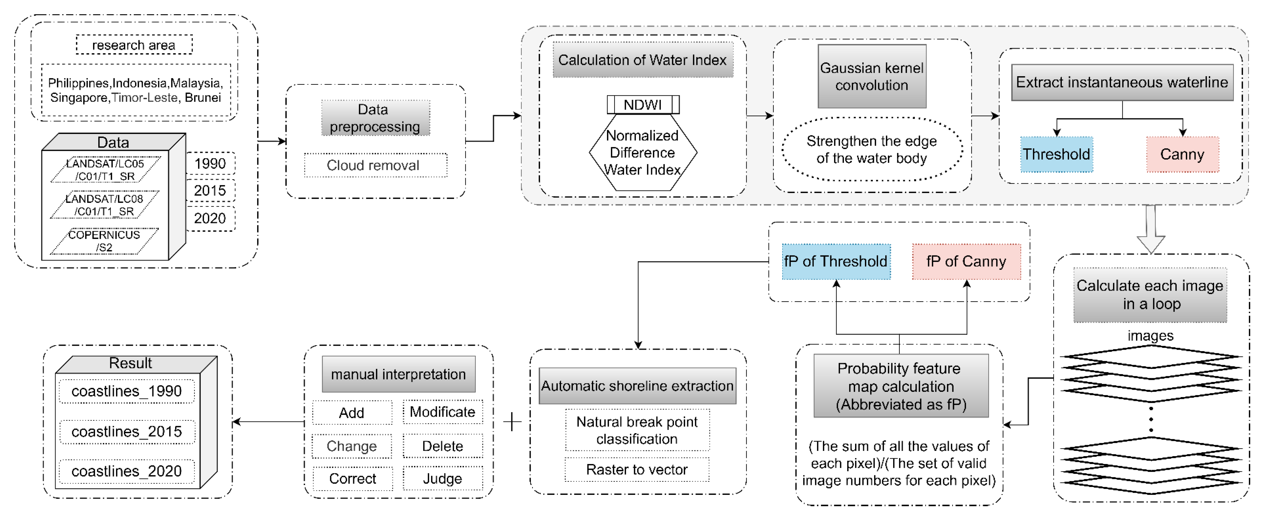
2.1. Data Source and Platform

Currently, many types of remote sensing image data are widely used in coastline dynamic monitoring because of their convenient access channels and relatively low cost. We selected the commonly used Landsat-series data as the basic data source. Until now, many scholars have used different types of remote sensing image data for their research. Some scholars [17,18,19,20] have applied the LiDAR technology with high-precision point cloud information to research work into the coastline. Obtaining full three-dimensional beach terrain data has made it possible to determine the location of the coastline on a regional scale, but LiDAR has a price. It is expensive, is susceptible to weather, and has a limited working distance. In view of the many disadvantages of radar images, optical remote sensing images, such as Sentinel [21,22], GeoEye [23], IKONOS [24], Pleiades [25], Spot [26], RapidEye [27], Landsat [9,28,29,30,31], and WorldView-2 [7,32], have been used by many scholars in coastline research and analysis. Different types of optical images, however, have distinct advantages and different application ranges. Considering that this research had the characteristics of large-scale time-series monitoring and the availability of long-term series of images, we selected the composite data of Landsat satellite imagery. This data source has the advantages of a long image time series, wide image size, a large range, high efficiency, and low cost. Regarding the research platform of this experiment, we selected the GEE platform developed by Google; it combines a large number of satellite images and geospatial datasets acquired for a long time with data processing and analysis functions. It not only solves the problems faced when downloading remote sensing data (time-consuming and labor-intensive), but also effectively avoids the complicated and tedious processing work caused by the huge amount of remote sensing image data. It also reduces the requirements for storage equipment and computer computing capabilities for scientists. Researchers and developers can use it to achieve better detection, supervision, maintenance, analysis, and prediction of the earth’s surface, especially for large-scale research of dense time-series remote sensing images [33]. The data source of this study in 1990 was Landsat-5 remote sensing image data, which included "LANDSAT/LC05/C01/T1_SR" on the GEE platform; in 2015 and 2020, the data source was Landsat-8 remote sensing image data, which included "LANDSAT/LC08/C01/T1_SR" on the GEE platform.

2.2. Coastline Extraction Method

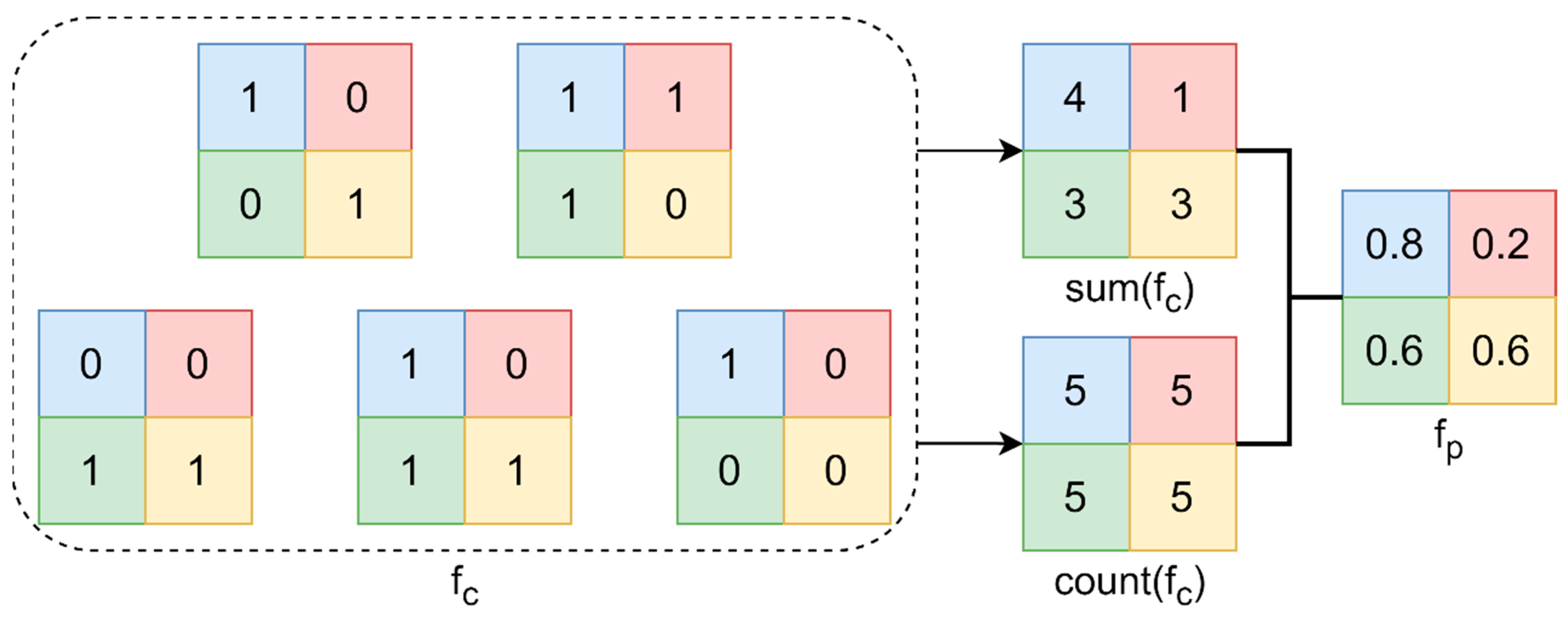
2.2.1. Method Overview

We proposed a unified standard coastline extraction method based on GEE and dense time-series remote sensing image data by calculating the probability of the waterline. This method mainly includes remote sensing image preprocessing, water index calculation, Gaussian kernel convolution, instantaneous waterline extraction, probabilistic feature map calculation, automatic coastline extraction, and manual interpretation. The main idea is to calculate the normalized difference water index (NDWI) of each valid image in a year through Otsu algorithm threshold segmentation and the Canny edge detection operator for edge detection, obtain the instantaneous waterline at all times of the year, calculate the frequency of edge occurrence to obtain a probability feature map, and extract the coastline automatically according to the final probability feature map using the natural discontinuity classification method. Combining the two results and the manual correction extracts the messy part of the data, and then the final shoreline result can be obtained. This method fully takes into account the impact of tidal-level variations, which are important for determining the average coastline from satellite data. The method not only effectively avoided the deviation caused by treating instantaneous waterlines as shorelines, but also did not require the support of many years of tide observation data and got rid of the dependence on average high-tide height data. Even in remote areas with sparsely populated, complex terrain and a harsh environment, an accurate coastline can be extracted, and the method can be widely used in a wide range. The workflow of this research method is shown in Figure 1.

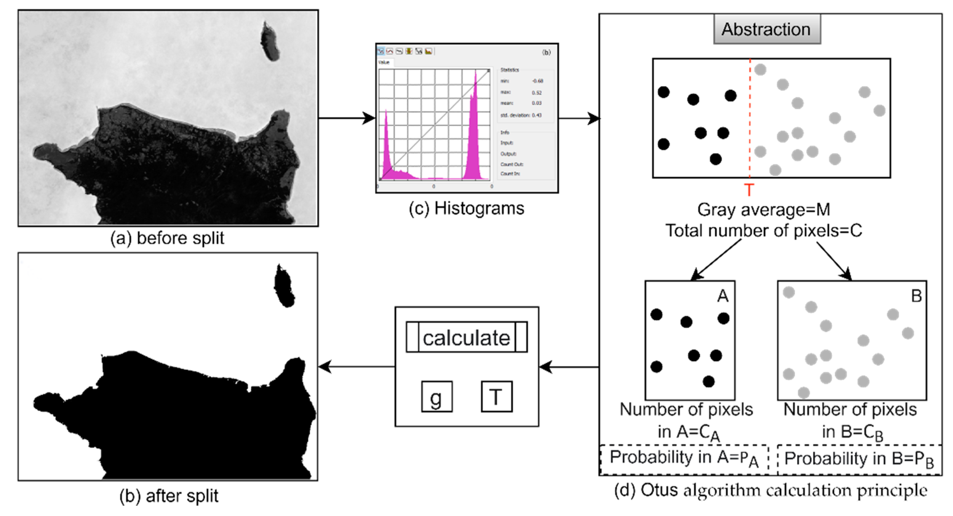
2.2.2. Specific Method

We introduced the specific extraction process of our method in detail. First, for each remote sensing satellite image, we reduced the interference caused by coastline extraction. Noise reduction was required for the image, and the noise generated by waves, ships, storms, atmospheric radiation, and other factors in the image, especially the interference of clouds, was eliminated on the condition that the features of sea and land edges were completely retained. Then, we calculated the Water Index. The NDWI uses the green band and near-infrared band to monitor changes related to water content in water bodies [34], and it is widely used in water research [35,36,37]. The principle is to use the reflected near-infrared radiation and visible green light to eliminate the characteristics of soil and land vegetation to enhance the contrast between water and land. After normalization, the image water body will show higher brightness in the image instead of the dark water body. The instantaneous waterline was extracted by calculating the NDWI. The calculation formula is as follows:
  N D W I = ( Green   band ) ( Near   infrared   band ) ( Green   band ) + ( Near   infrared   band )
After calculating the water body index of all the effective images in a year, we used a Gaussian kernel to filter the water body to prepare for the next stage of edge detection. This method used a Gaussian kernel for convolution. The Gaussian distribution was a normal distribution [38], which had the largest central value—the farther away from the central value, the smaller the value. The two-dimensional Gaussian formula is as follows:
G ( x , y ) = 1 2 π σ 2 e ( x 2 + y 2 ) / 2 σ 2
The principle of Gaussian kernel convolution is to make the image produce a "blur" effect, that is, to make each pixel obtain the weighted average of the surrounding pixels, thereby enhancing the characteristics. When calculating the weighted average, we used the "center point" as the origin (0,0) to calculate the coordinates of other points. If the radius was 1, the coordinates of the point on the right side of the "center point" were (1,0). According to the point coordinates and Gaussian formula, we calculated the weight, assigned the weight, and then multiplied and added the corresponding weight value of the pixel and the original image pixel value to obtain the new pixel value and the convolution feature value. We performed convolution smoothing to obtain an image with new pixel values, and the edge features of the image were enhanced, which was conducive to more accurate contour extraction. The image extraction effect after Gaussian convolution is shown in Figure 2a,b, and the convolution process is shown in Figure 2c.
We used two methods to extract the instantaneous waterline. In the first method, we used NDWI to normalize the image and then used the threshold segmentation method to extract the shoreline. The threshold segmentation method had the advantages of high efficiency, fast speed, and simple and easy operation. It is based primarily on the different pixel gray values of the target object and the background object, and the two are separated by setting a reasonable threshold. As the segmentation result depends on the setting of the threshold completely, the determination of the threshold is important. We used the Otsu algorithm (maximum between-class variance method) [39] to calculate the optimal threshold. Taking Panultan in the Philippines and the part of Papua south of its location as an example, the normalized NDWI image of this area is shown in Figure 3 (shown in the "before split" picture in a), and assuming that the normalized image is composed only of foreground and background colors, the land is the foreground color and the water body is the background color. We calculated the grayscale histogram of this image, which is shown in Figure 3 3b, in which the low peak is the foreground color, and the peak represents the background color. Its average gray value is denoted as ‘M,’ and the total number of pixels is denoted as ‘C.’ Assuming that there is any gray value, ‘t,’ take the foreground color of the histogram and background color segmentation and mark the separated two parts as ‘A’ and ‘B.’ The corresponding gray values are ‘MA’ and ‘MB.’ The number of pixels in each part is recorded as ‘CA’ and ‘CB.’ The ratio of the part of the total number of pixels is denoted as ‘PA’ and ‘PB,’ and the Otsu formula can be expressed as follows:
P A = C A C ; P B = C B C , g = P A ( M A M ) 2 + P B ( M B M ) 2
When the value of ‘t’ changes, the ratio of pixels corresponding to the two parts ‘A’ and ‘B’ and the average gray value also change. When ‘g’ reaches the maximum value, the segmentation effect is the best, as shown in Figure 3c; the ‘t’ at this time is marked as ‘T.’ ‘T’ is the best threshold.
The second method is edge detection. Because threshold segmentation has certain drawbacks, the extraction results of some complex regions were not ideal. Therefore, we introduced the edge detection operator to comprehensively compare the results of threshold segmentation to ensure the accuracy of the results. This combination of the two methods has been recognized by many scholars [40,41]. Edge detection operators include Roberts, Prewitt, Sobel, Laplacian, LoG, Canny [42], and other different detection operators. These operators have different algorithms and application fields and are widely used in image processing and computer vision. Kumar et al. [43] concluded that among many types of operators, the Canny edge detection operator performs better than all other edge detection operators in all aspects. For example, it is inherently adaptive and especially suitable for noisy images, and its false edge detection probability is low. The same conclusion was reached in a study by Maini et al. [44]. Therefore, this research used the Canny operator for edge detection. The threshold of the canny operator should be reasonably selected for images of different quality. Different thresholds produced different extraction effects, as shown in Figure 4. Generally, the smaller the threshold, the richer the extracted details. When the threshold was large, some smaller islands were easily overlooked, making it more likely that the extraction result would be blank, as shown in Figure 4d.
Because this method is not suitable for single-scene images, but rather for all images in a year, this processing and calculation should loop through each image, obtain the pixel feature value of each image, and calculate the probability after integrating all the feature values. The process of obtaining the unique value is the calculation of the probability characteristic value, as shown in formula (4):
f p = sum ( f c ) count ( f c )
where fP represents the probability, and fc represents each pixel in the image. We used the sum to calculate the sum of all the values of each pixel and used the count to calculate the set of effective image numbers for each pixel. The schematic diagram of the calculation process is shown in Figure 5.
Finally, according to the extracted probability feature map, we selected the natural breakpoint classification method (Jenks) [45] to realize automatic extraction of the coastline. The natural discontinuity classification method is a data clustering method, whose principle is to minimize the average deviation between each class, maximize the deviation between each class and the mean of other classes, and set the boundary at the position where the difference of data value is relatively large. According to this principle, automatic coastline extraction can be realized based on a probability feature graph. We vectorized the calculated boundary values, and the vector data were more conducive to the superposition analysis of shoreline than the raster data.
Automatic coastline extraction results need manual interpretation. We combined the shoreline extracted by NDWI threshold segmentation and the shoreline detected by the Canny operator to determine the specific location of the shoreline. In our results, most of the shoreline NDWI threshold segmentation and extraction results were consistent with the detection results of the Canny operator. In the coastline extraction work, we found the following problems: the island’s NDWI extraction results fit well with the Canny detection results, and the two results had different degrees of deviation in the complex coastline. For rivers, the results of the Canny detection operator were relatively good. The NDWI extraction result data were cumbersome, and the extraction of more complex shorelines with marine aquaculture projects, port transportation gates, and muddy textures required manual visual interpretation to determine the specific location. As the impact of different types of coastlines was not considered, there were some shortcomings in the extraction results. To reduce the interference caused by these shortcomings, we adopted the following reference standards:
1. When both threshold segmentation and Canny operator methods show good results, threshold segmentation is used as the standard, and the Canny operator detection result is used as an auxiliary judgment;
2. In the case of large deviation of the two results, artificial visual interpretation is adopted, and the Canny results prevail;
3. In small areas with poor Canny results, we modify and supplement the derived raster image, and if necessary, refer to remote sensing satellite images for reasonable judgment; and
4. Regarding the treatment of the estuary, we use the estuary treatment results of Liu Chuang et al. [46] as the basis, which can avoid the impact of estuary treatment differences in the later accuracy verification.
When refining the coastline, we employed the following major operations related to coastline precision processing:
  • Supplement the missing smaller islands.
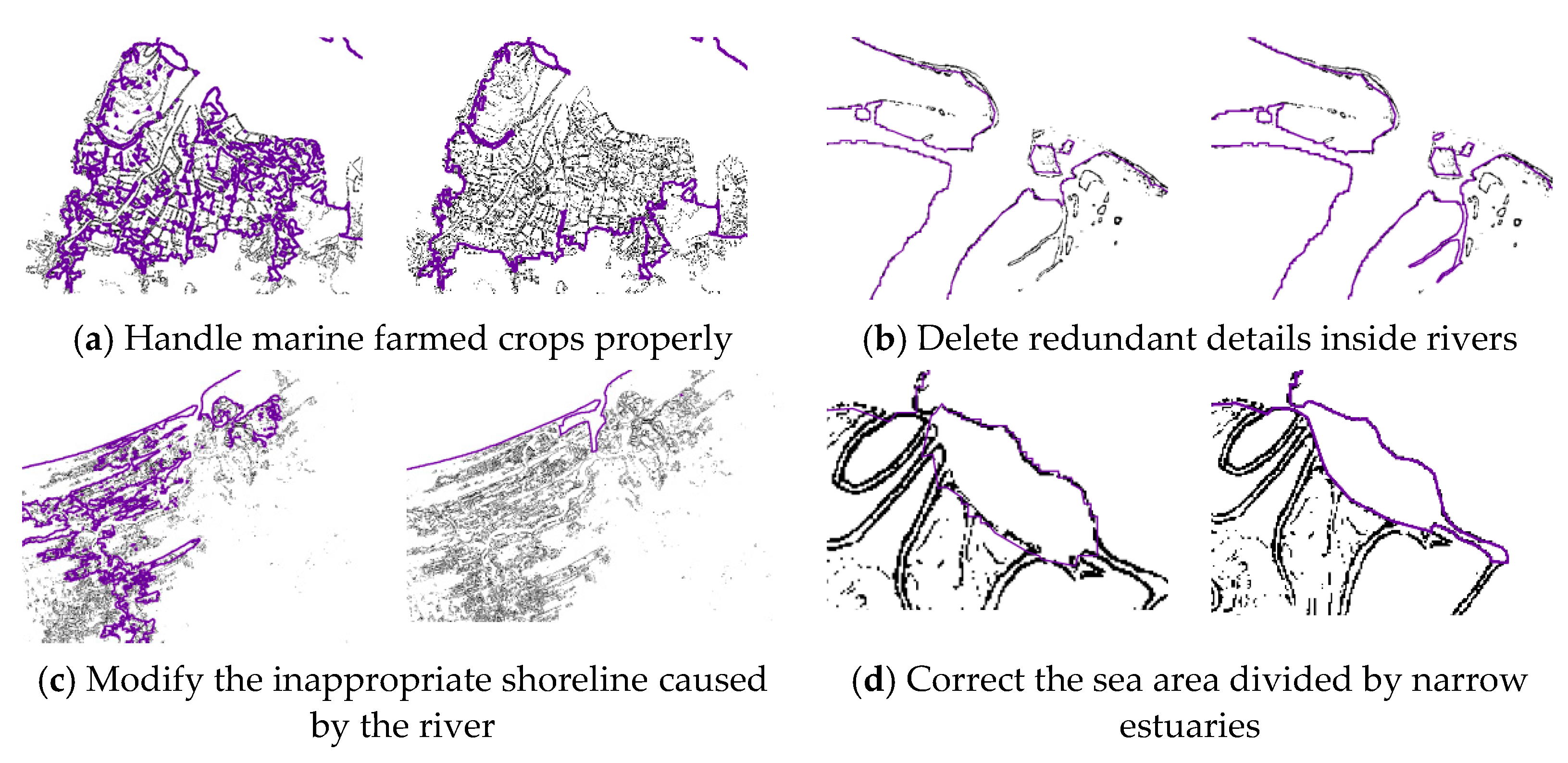
  • Modify the inappropriate shoreline caused by the river.
  • Change the wrong land extraction inside the river.
  • Delete the extra incorrect islands.
  • Correct the incorrectly drawn islands connected to the land.
  • Delete redundant details inside rivers.
  • Handle marine farmed crops properly.
  • Distinguish the border of inland rivers formed by seawater inflow reasonably.
  • Supplement the coastline that has not been extracted for some reason.
  • Correct the sea area divided by narrow estuaries.
  • Draw simple and practical shorelines for complex coastal features reasonably.
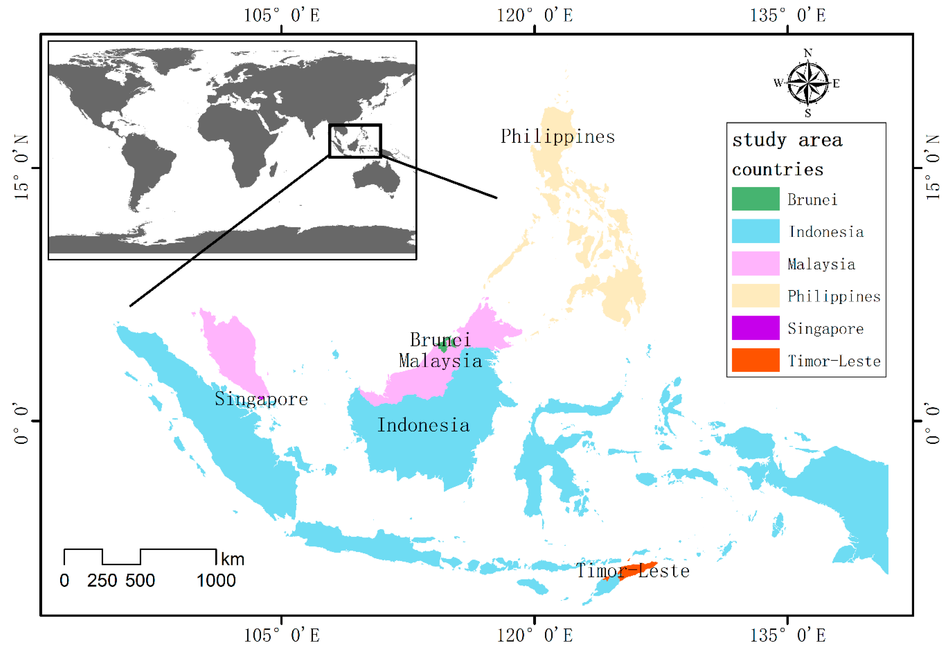
The parts of the coastline that were corrected accurately by manual work changed in different degrees. The schematic diagram before and after processing is shown in Figure 6.

2.3. Study Area

To verify that the application of this method to extract the coastline offered the advantages of the uniform method, high accuracy, and large-scale application, we selected the Malay Islands region, with many islands and a complex coastline structure, as the research area. The research area included six countries: the Philippines, Indonesia, Malaysia, Singapore, East Timor, and Brunei.
Since the 21st century, the Malay Islands, represented by countries such as Singapore, the Philippines, and Indonesia, have developed rapidly and received extensive attention from around the world. The region has a hot and humid climate, rich tropical forests, and unique natural advantages. It is considered to be one of the most sensitive and fragile areas [47]. In addition, it is a densely populated area, with many islands and rich marine resources. The region is ideal for research because of its numerous islands and complex coastline composition. In the context of rising global temperatures and rising sea levels [48], the analysis of temporal and spatial changes in Southeast Asia can enhance our awareness and understanding of the changing trends of the Malay Islands and the global oceans and islands. The region also provides a certain reference value for marine research. A schematic diagram of the selected study area for this shoreline extraction is shown in Figure 7.

2.4. Missing Data Supplement

During the coastline extraction process in 1990, the data of ‘LANDSAT/LT05/C01/T1_SR’ could not fully cover the study area. As a result, the extraction results in 1990 were not ideal compared with the results in 2015 and 2020. We supplemented the data with T2 images from the same period and images from other times similar to this period. The 1990 T2 image “LANDSAT/LT05/C01/T2_TOA” could supplement a large area of uncovered area, but the T2 image quality was poor. In line with the principle of improving accuracy by reducing the period as much as possible, and based on maintaining a good application of the extraction method of this research and reducing the workload of manual modification, our first choice was to use images from 1986–1995 to supplement year by year. The specific supplementary areas and the data used were as follows: The 1986 T1 level images were used to supplement the Papua, Camiguin, and other areas in the Philippines. The 1987 T1 level images were used to supplement the Philippine’s Palawan, Puerto Princesa, and Wakatobi in Indonesia National Park and other regions. We used the 1988 T1 level images to supplement the Philippines Catanduanes, Busuanga and other regions. We used 1989 T1 level images to supplement Indonesia’s Biak, Serui, and other regions. We used the 1991 T1 level images to supplement Indonesia’s Celaya, Muna, Batton, and other regions. We used the 1992 T1 level images used to supplement Indonesia’s Nabire and other regions. We used the 1993 T1 level images to supplement Indonesia’s Moyo, Murdun and other regions. We used the 1994 T1 level images to supplement the Central Philippines’ Tablas and Sibuyan, Basbat, Cebu, Mindanao, Bohol, Davao, and other regions. According to the supplementary results, there were still coastlines in Basco in the Philippines, Nias, Batu, Sibilu, Mentawai, Bali, and West Nusa Tenggara in Indonesia. We used T2-grade images in 1990 for supplementary data.

3. Verification and Application

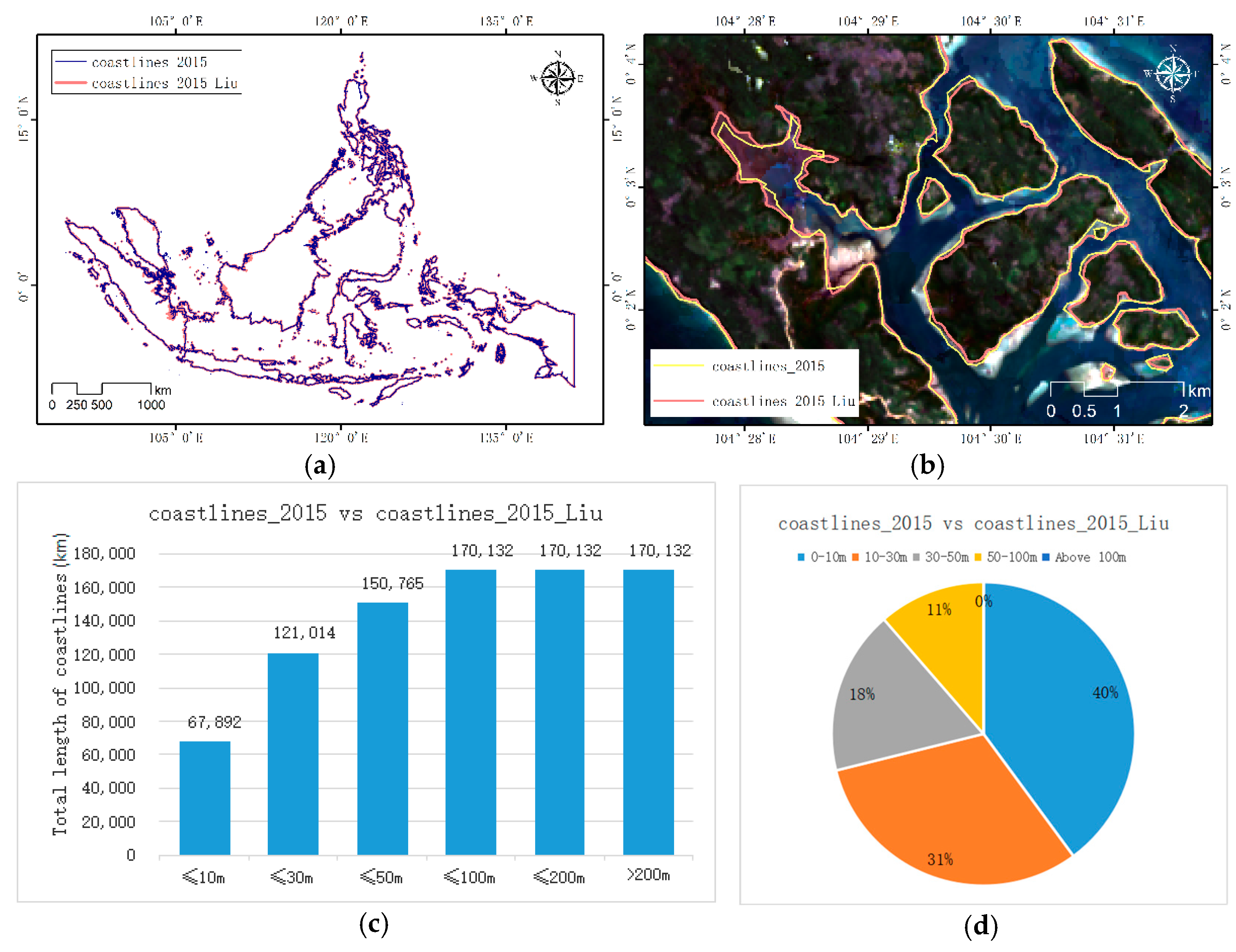
3.1. Consistency Comparison between Coastline Extraction Results and Other Data Products

Using the semiautomatic coastline extraction method, which is proposed based on GEE and dense time-series remote sensing image data, we obtained data from the Malay Islands region for 1990, 2015, and 2020. The results were denoted as "coastlines_1990," "coastlines_2015," and "coastlines_2020." Because of the large area of this study, the cost of fieldwork was high. Considering that many scholars have carried out research on the coastline and have produced relevant data, we compared the extracted results with the existing data. The comparison method was the buffer superposition method. The specific operation was to establish a buffer zone based on published data that are widely recognized and to perform superposition analysis with the data produced by this method. The buffer distances were 30 m, 50 m, 100 m, and 200 m. The accuracy of the coastline result was judged based on the total length of the intersection of the coastline and the buffer zone.
Considering that the coastline will change because of natural factors, such as sedimentation, seawater erosion, global warming, and human-made factors (e.g., port construction, land reclamation, and marine engineering) [20,49,50], the coastline at different periods also may change. Great changes likely will occur. Therefore, when selecting data, the "same time" became the primary key factor. We chose coastlines extracted during the same period to improve the accuracy and reliability of the accuracy verification method. We also considered the breadth and accuracy achieved by the data.
Currently, two main global coastline thematic products are widely used. They are “coastlines_2015_Liu,” produced by Liu Chuang and others [46] and published in Journal of Global Change Data and Discovery, and the “coastlines_OSM,” published in Wiki World Map (https://wiki.openstreetmap.org/wiki/Coastline, accessed on 12 August 2021). The “coastlines_2015_Liu” data included coastlines artificially produced by Liu Chuang and others based on GEE’s highest spatial resolution meter-level remote sensing image. The data take into account different types of coastlines and combine topographical factors. Moreover, 85% of the total data has 20 m accuracy and a download volume of up to 5013, which indicated that had high applicability and credibility. In this study, "coastlines_2015" also was based on the production of remote sensing images in 2015. We used a comparative analysis of these two types of data to eliminate the impact caused by the difference in time. If "coastlines_2015" and "coastlines_2015_Liu" had a relatively high degree of coincidence, the result of "coastlines_2015" was as reliable as "coastlines_2015_Liu." Also, the "coastlines_1990" and "coastlines_2020" coastline results and the "coastlines_2015" coastline results were produced using the same method, so the accuracy of the "coastlines_2015" coastline indirectly indicated that the other two periods also achieved higher accuracy. The accuracy assessment result of the method used in this experiment is shown in Figure 8.
We did a superposition analysis of the "coastlines_2015" data result extracted in this study and "coastlines_2015_Liu." As Figure 8c shows, a total of 67,892 km of coastlines and "coastlines_2015_Liu" data results were within the accuracy range of no more than 10 m. Moreover, 67,892 km represented 40% of all coastline lines (Figure 8d). Additionally, the 150,765 km coastlines were within the accuracy range of no more than 50 m from the 2015 data standard. All the extracted results were within the range of the location deviation of no more than 100 m, and the error of 89% in the results was no more than 50 m. Furthermore, the "Coastlines_2015" data results and "coastlines_2015_Liu" data results were in good agreement. Therefore, from the results of the accuracy assessment, we concluded that the overall accuracy of the coastline extracted by this method had a higher coincidence degree of less than 100 m compared with the widely used data that have been published to date. The accuracy of the results also was good, and thus, these results can be used in the analysis of temporal and spatial changes in the Malay Islands.

3.2. Dynamic Monitoring of the Malay Islands Coastline

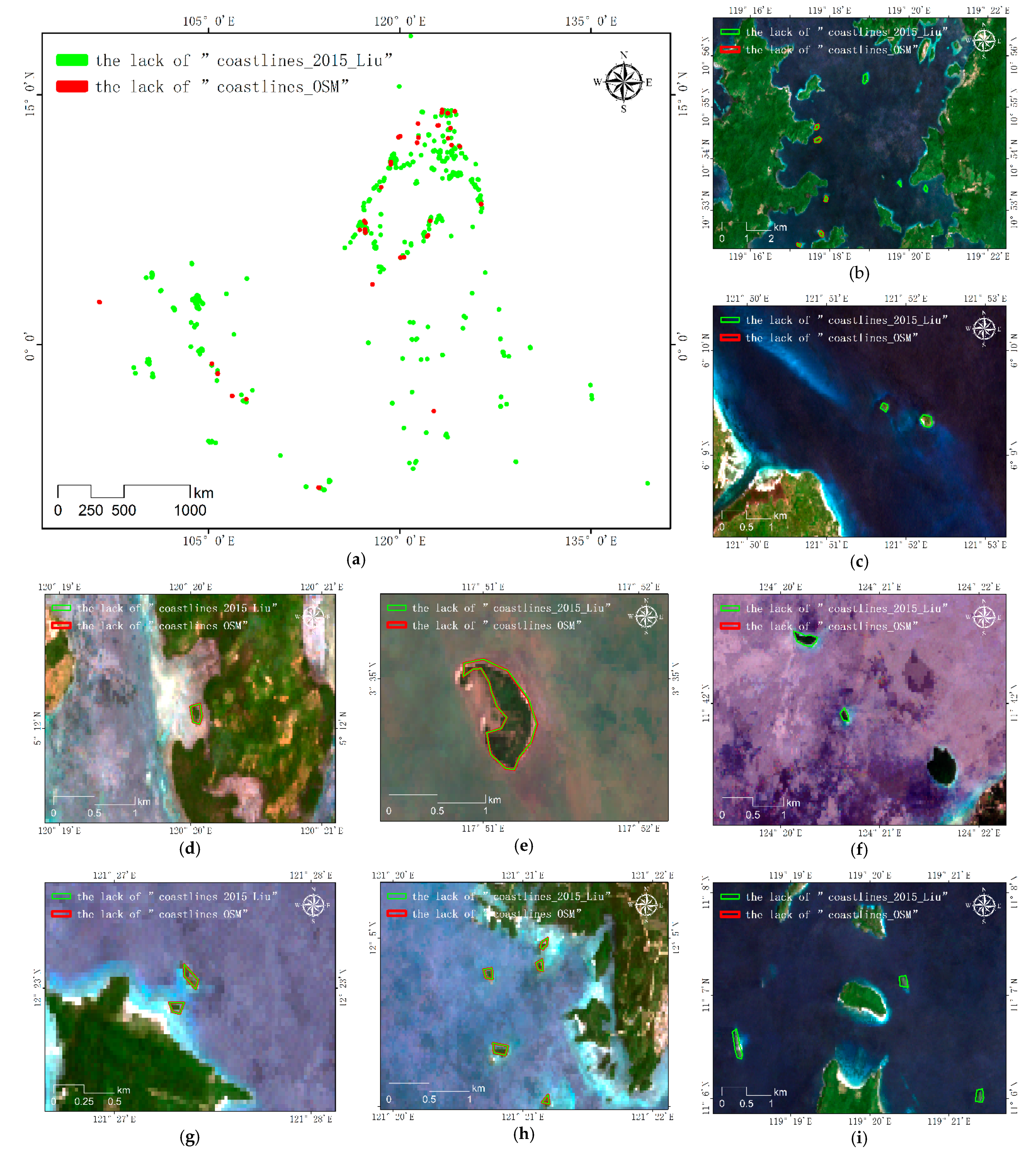
3.2.1. Islands Data Supplement

This method offered the advantage in the extraction of islands and reefs, and the results indicated comprehensive island and reef data. By superimposing and analyzing the two datasets of "coastlines_2015_Liu" and "coastlines_OSM," this study made up a total of 96 islands that were missing from both datasets, among which up to 813 islands were missing from "coastlines_Liu_2015." It can be seen from the supplementary islands’ data that the extraction method based on dense time-series remote sensing images can avoid the lack of data on islands and reefs that are easily submerged by seawater. In the context of rising global temperatures and rising sea levels, this is of great significance for the use of remote sensing images for long-term serial monitoring of coastlines and islands. Comparing the three-phase data results of "coastlines_1990," "coastlines_2015," and "coastlines_2020," extracted in this study with the data results of "coastlines_2015_Liu" and "coastlines_OSM," we found that many islands existed but were not recorded by the current public data. After manual discrimination and combination with remote sensing images, we obtained the supplementary data of all missing islands. From the geographical distribution of missing islands and reefs, we identify that they were concentrated in the Philippines. This phenomenon can be seen in Figure 9a. According to statistics, a total of 813 islands with missing data from "coastlines_2015_Liu" were added, with a total area of 273.99 km2. Among them, the smallest island was only 251.33 m2, and the largest island was as high as 135.01 km2. The data missing from "coastlines_OSM" represented 96 islands with a total area of 205.73 ha.
According to the phenomenon of some islands missing “coastlines_2015_Liu” data, and “coastlines_OSM” data not missing, we concluded that data of “coastlines_2015_Liu” could be drawn manually with higher accuracy. The data had a significant shortcoming that is easy to miss compared with automatic extraction. The islands that were extracted by others revealed the shortcomings of the single-scene image extraction coastline. When the sea level rises, the islands and reefs will be submerged, and some new islands and reefs will be exposed when the sea level drops. These uncertain factors can be minimized when extracting the coastline from dense time-series remote sensing images. Of course, some islands and reefs also may be newly formed because the earth has a complicated geographical structure and geological conditions. Every time the qualitative conditions change, some new islands will be formed. For example, changes in plate tectonics, the melting of glaciers, and the eruption of volcanoes may all create new islands. To further verify the real existence of the new islands discovered through data overlay, the corresponding remote sensing images were confirmed one by one. The details of some islands are shown in Figure 9b–i.

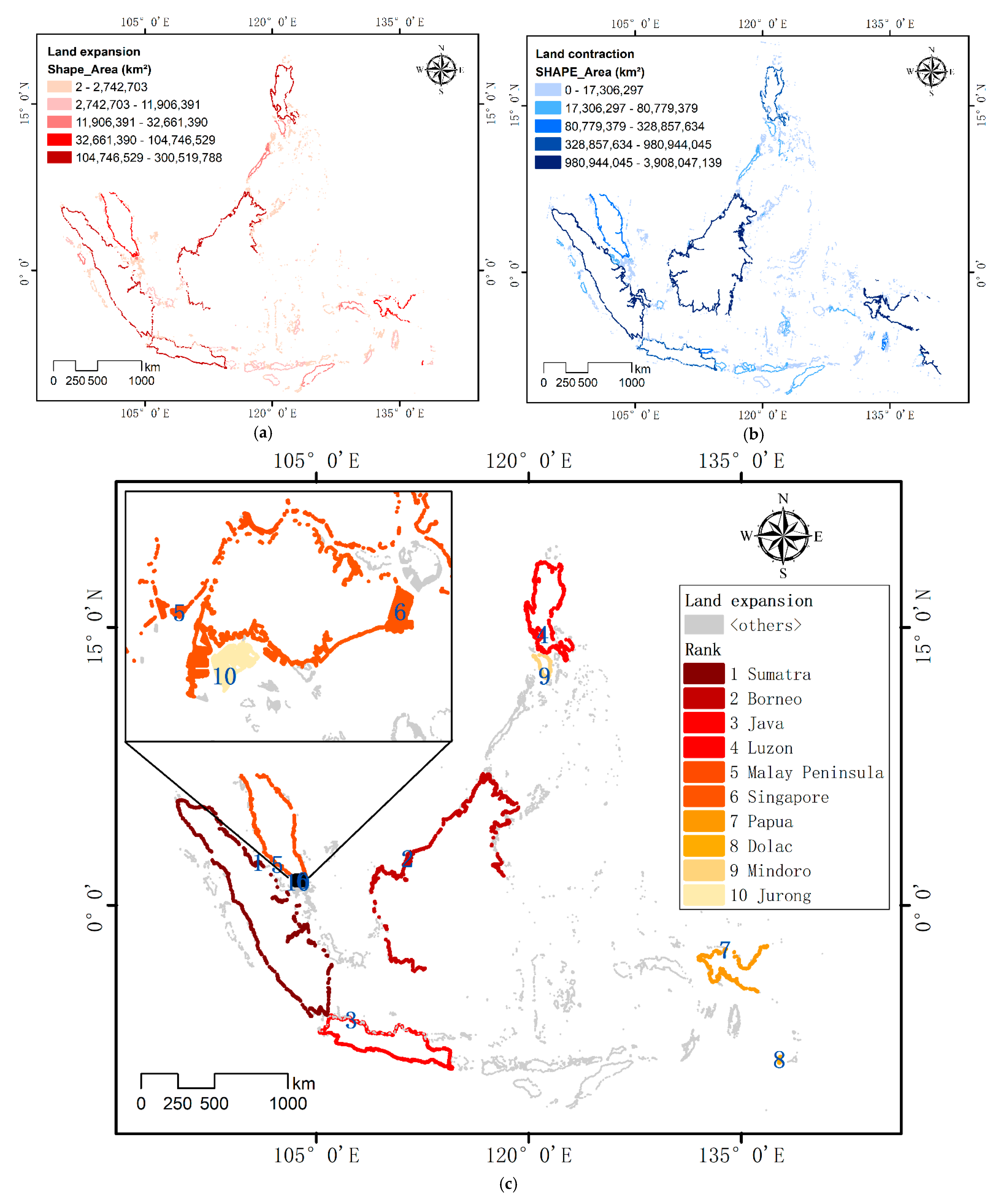
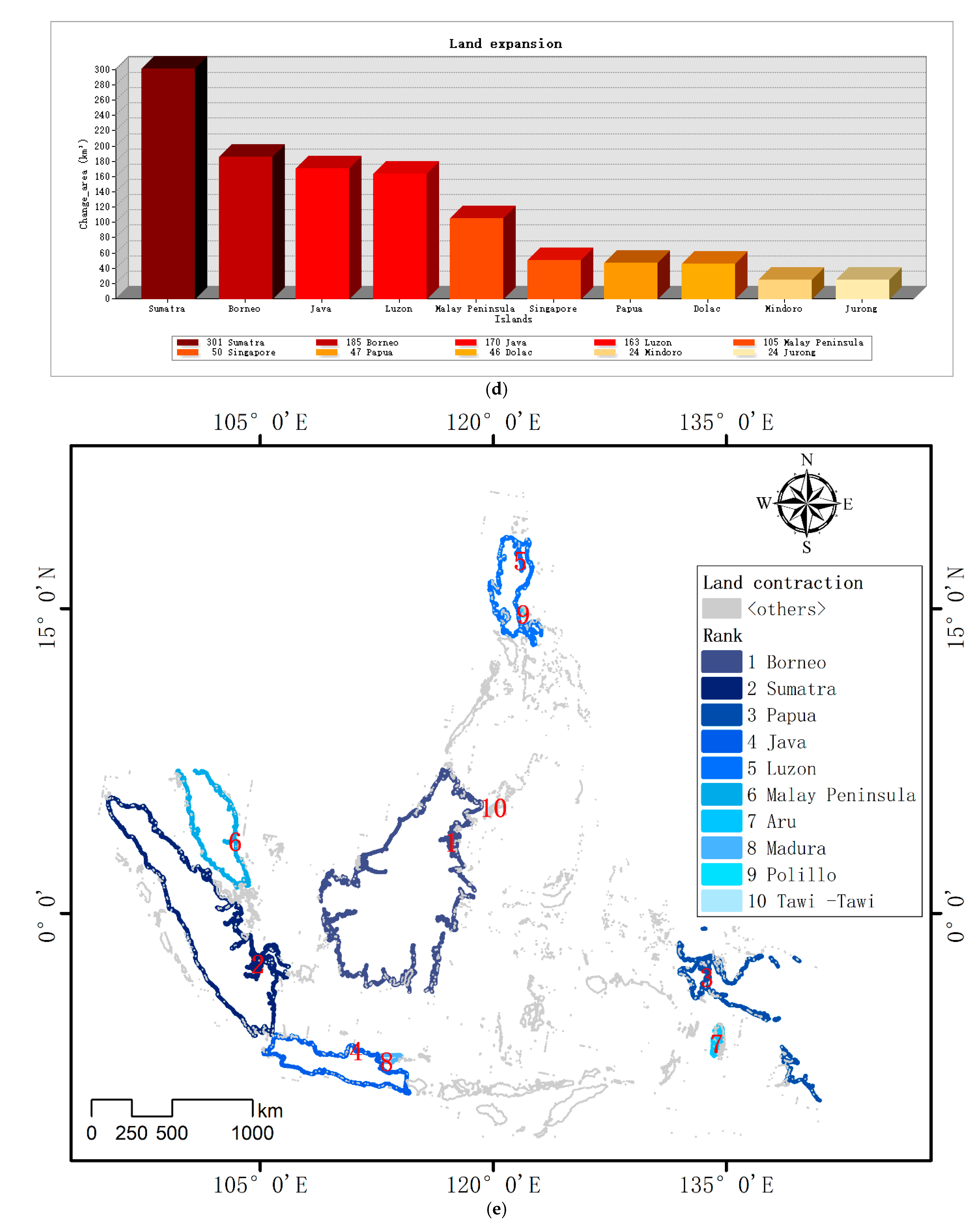
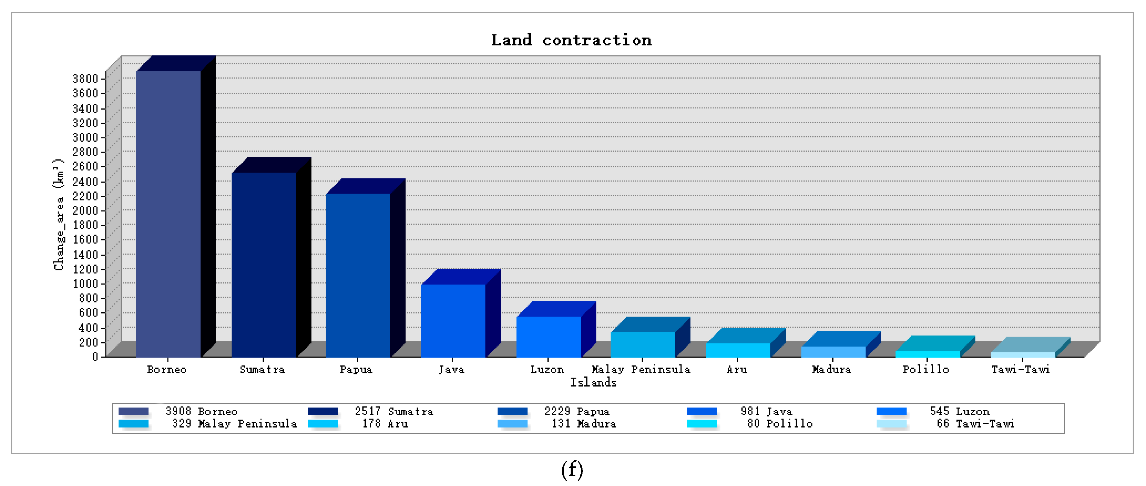
3.2.2. Expansion and Retreat of Coastlines

As the quality of the image may have a certain impact on the extraction results, the increase in the length of the coastline does not mean an increase in the land area. On the contrary, the increase in the length of the coastline is likely to be accompanied by a decrease in the area of the landing area, and the changes between the two are often inconsistent. For example, when reclaiming land in the bay, the length of the coastline likely will be reduced. When the waves continue to wash and erode the island to change its shape, or when an artificial port is built in a relatively smooth coastline area, it may lead to an increase in the coastline. This means that the erosion trend of the coastline will be offset by an increase and change in the surrounding coastline [51]. Therefore, the changes of the overall coastline are greatly affected by various influencing factors, and the fluctuation of the coastline causes the relevant changes to the land plate. This section reveals the changes in the coastline indirectly from another angle, namely land area changes.
According to the superposition analysis of the land area of the entire study area, it is known that land expansion and land contraction coexist. Generally, the land area showed a shrinking trend. Among these changes, the changes in the Indonesian Islands were the most significant. Whether it was land expansion or contraction, the Indonesian Islands showed a more obvious trend of change than did the Philippine Islands. As shown in the red area in Figure 10a,b, the large islands in Indonesia expanded and contracted to a certain extent. Among these changes, the changes in Borneo were more obvious. In addition, Luzon and Palawan in the Philippines also showed significant expansion and contraction. Compared with the islands in the southeast of the Philippines and the Sulawesi and surrounding small islands, these changes were minimal. This conclusion was the same as the research results in [11]. As shown in Figure 10a, Indonesia Island, North Borneo, Palawan, and Luzon on the west side showed an expansion trend, and they were all close to the Eurasian continent. We inferred that the main reason for this phenomenon may be that the Philippines, Indonesia, and Brunei are all major import and export countries. The development of foreign trade has increased the demand for port construction, and the economic development brought about by trade has indirectly led to population migration. This increase in population has increased the demand for land area. Therefore, human activities, such as land reclamation, coastal aquaculture, and port construction, have had a greater impact on the coastline. Compared with the obvious expansion trend of North Borneo, almost no land expansion phenomenon was evident in South Borneo. However, we did observe a certain contraction trend. Combined with the changing trend of Sulawesi, we inferred that Sulawesi in Indonesia is the center, and the surrounding islands include Taliabu, Bulu, Bazan, Weta, and Yan. Many islands, such as Denali and South Borneo, have been eroded by seawater. Thus, to a certain extent, we identified a phenomenon of reduced island area. The specific changes are shown in Figure 10b.
Using natural islands as a benchmark, the statistical results are shown in Figure 10c,e. The top 10 regions with the most obvious expansion were Sumatra, Borneo, Java, Luzon, the Malay Peninsula, Singapore, Papua, Dolac, Mindoro, and Jurong. The top 10 regions with more obvious contraction were Borneo, Sumatra, Papua, Java, Luzon, Malay Peninsula, Aru, Madura, Polillo, and Tawi-Tawi. The specific change area is shown in Figure 10d,f. Among them, Sumatra is a well-known volcanic island. It is located in the Eurasian seismic zone and belongs to the high-earthquake area. Earthquakes occurred in many recent years, such as 2004, 2009, 2010, and 2012, and were accompanied by relatively strong tsunamis. Even the highest tsunami reached 10 m, which greatly damaged the environment of the coastal area, and the post-disaster restoration also had an impact on the coastline. The central part of Borneo has many mountains and high altitudes. Its topographical factors give it an extremely uneven population distribution. Because the coastal areas have the advantages of convenient transportation and suitable temperature, the population is mainly concentrated in the coastal areas, and human activities have significantly affected the distribution of the coastline of Borneo. According to these findings, human activities have produced larger impact on coastal areas. Compared with the obvious changes in local areas brought about by human activities, the changes in the position and shape of the coastline caused by natural forces are often large and small.

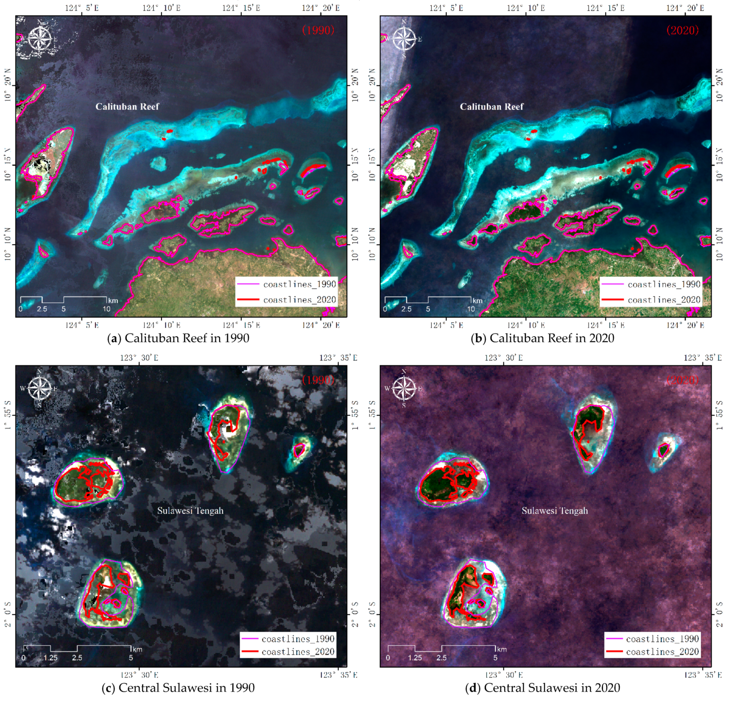
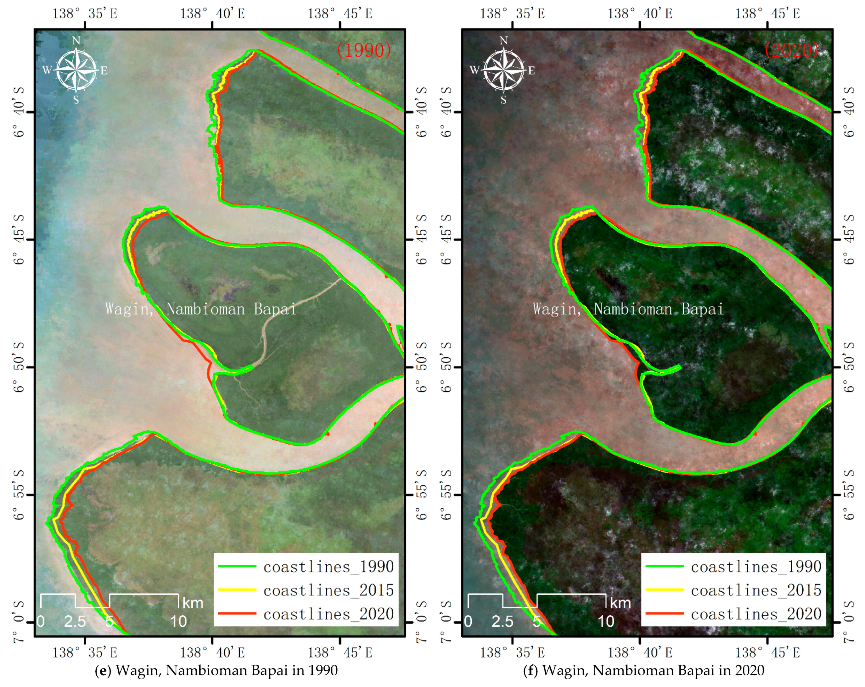
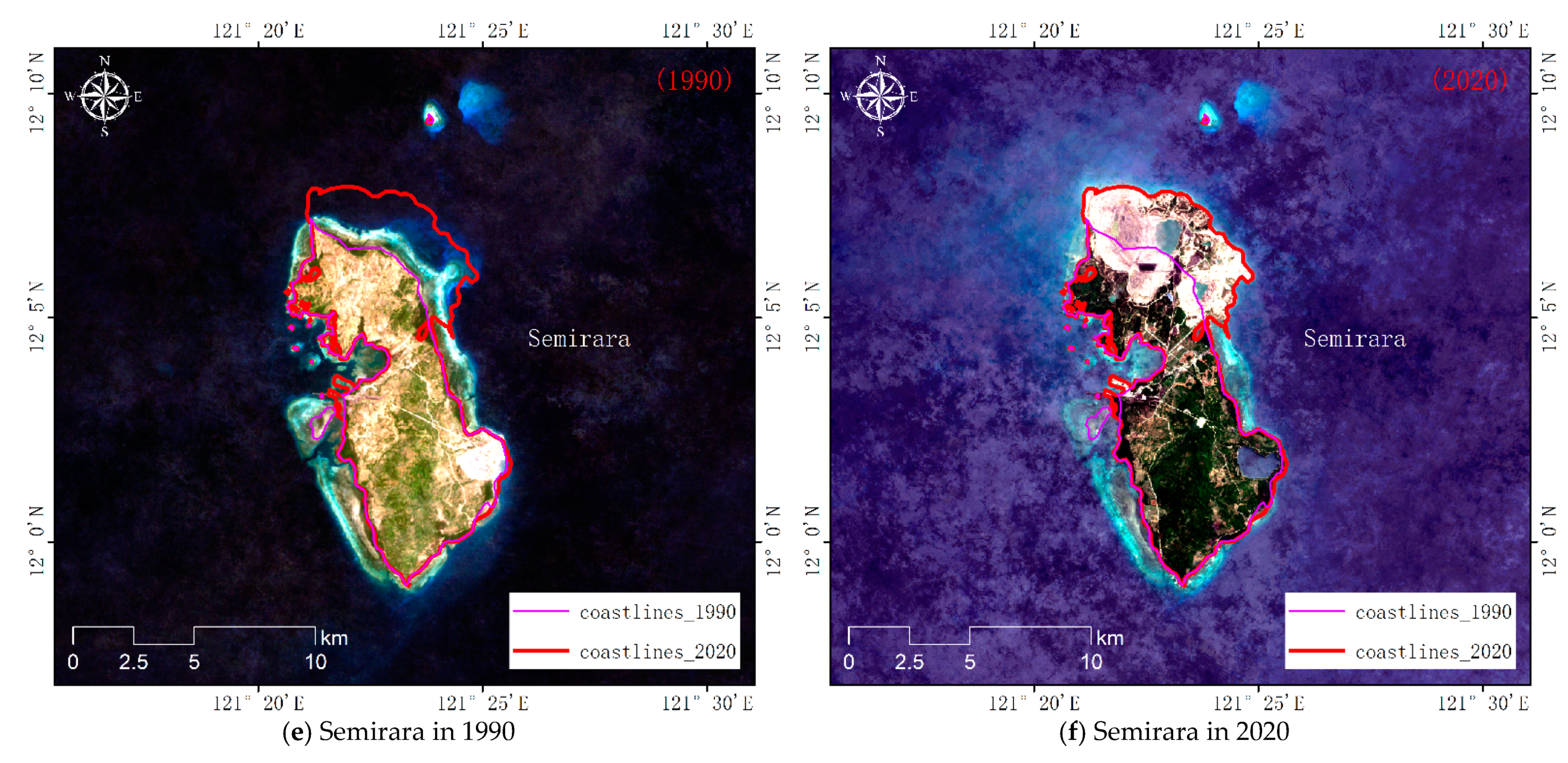
3.2.3. Analysis of Typical Change Areas

The large-scale spatial differences of land are reflected to a large extent at the local area and single island level. Tidal action makes seawater fluctuate, and the constant friction between seawater and land will affect islands in the ocean, especially small islands and reefs. Therefore, for inconspicuous small atolls or reef islands, the geographical and morphological differences brought about by time cannot be underestimated. Tidal action, coupled with natural forces such as temperature, rainfall, storms, tsunamis, and volcanoes, mean that many changes in the sea on the islands and reefs remain unknown. The changes brought about by natural forces are often minimal and take a long time to accumulate, whereas human behavior will cause major changes to the island in a short time. We analyzed the factors that cause changes in coastlines and islands and categorized them into two major driving factors: natural factors and artificial transformation.
  • Changes driven by natural factors
Under the influence of natural factors, the area of Calituban Reef in the Philippines increased over the study period; in contrast, the islands of Central Sulawesi and Papua in Indonesia were eroded by seawater. Figure 11a,b shows the Calituban Reef, with the Olango on the left, which belongs to the province of Cebu in the Philippines. This area has a hot and humid climate [52]. Comparing the extraction results in 1990 and 2020, the area of some islands and reefs in the Calituban Reef increased, and new smaller islands and reefs surfaced. This area has little human activity, but it has one of the most productive ecosystems on the planet, namely coral reef resources [53]. Comparing the coastlines of different periods, we found that the island group on the east side of Central Sulawesi in Indonesia was severely eroded by seawater, from a relatively complete and round landmass 30 years ago to a less regular shape. This complex structure is shown in Figure 11c,d. In 2018, Indonesia in Sulawesi Province Dongala county had an earthquake with an intensity of 7.4, which was accompanied by a tsunami. Road traffic, water, the electricity system, and communication engineering were nearly shut down in many areas. It lost contact with the outside world, which made it become an "isolated earthquake island" [54]. The impact of the earthquake and tsunami was huge and is a possible reason for the changing shape of the island. In addition, the coastline of Nambioman Bapai in Indonesia [55] was also severely eroded, showing a serious coastline retreat trend (Figure 11e,f). The "coastline" in this case is not really a coastline, but may be the observation line of the submerged mangrove forest. From 1995 to 2015, the mangrove line receded, and the mean and high waterlines probably receded by the same amount. This observation needs to be verified by additional investigations.
2.
Changes driven by human factors
With the development of human industrial civilization and the continuous increase in human needs, sea reclamation has appeared around the world. Although reclamation will bring a lot of convenience and development, it also will have an impact on the entire marine ecosystem. For example, we can expand the existing land area to meet the demand for land for port construction, dock size increases, the port industry, and marine aquaculture. Another human effect on the position of the coastline is the extraction of groundwater. These specific human activities cannot be seen directly from remote sensing images, which require further investigation and verification. These phenomena, while bringing economic benefits, break the natural balance between the coast and the seabed [56], destroy marine ecology, and change the hydrodynamic environment, putting the global ecosystem in danger [57].
Through the comparison of the data of the three phases, we found that the reclamation phenomenon in the islands of Java, Singapore, and Semirara was more significant. As early as 1991, Glaser et al. [58] proposed that Singapore’s land reclamation was as high as 10% of its land area at that time. As shown in Figure 12a,b, in the past 30 years, Singapore’s reclamation has been particularly obvious, especially on Jurong, which is the center of Singapore’s oil refining. As an artificial island, the area of Jurong increased by nearly 24 km2 from 1990 to 2020, and Singapore’s Changi and Queenstown areas had an obvious expansion. This phenomenon also can be seen in the Semirara in the Philippines (Figure 12e,f). In the Semirara, geographical topography is mostly hilly, with heavy rainfall and high temperature. Its economic construction is mainly based on the coconut industry, coal industry, and fishery. In recent years, fishery has developed and become prosperous. Fishery cultivation in this area is likely to increase the demand for island areas, which may cause it to expand the island Java is the island where Indonesia’s capital Jakarta is located. It is an important population settlement. Whether it is in the political or economic fields, it has a leading position in the country. As shown in Figure 11c,d, the eastern land area of Java has a clear trend of reclaiming land from the sea, and the phenomenon of artificial transformation is obvious.

4. Conclusions and Discussions

The coastline has always received extensive attention from scientific research and international fields. In the context of global warming and rising sea levels, more studies and analyses have been conducted on the location and morphology of coastlines and islands. However, because of the lack of good data and large-scale research and analysis, some inferences about the changing trend of coastlines have not been well verified. Studying the temporal and spatial changes of the coastline of Southeast Asian countries in the past 30 years is conducive to enhancing our understanding of the coastal areas of Southeast Asian countries.
To address the problem that the standard for extracting coastlines from remote sensing images is difficult to unify, this paper proposed a semiautomatic coastline extraction method based on GEE and dense time-series remote sensing image data to calculate the unified standard of the probability of waterline. This method fully considered the seawater climax lines at different times, integrated the two basic methods of NDWI threshold segmentation and the canny operator, and combined visual interpretation to obtain the coastline vector data of the Philippines, Malaysia, Indonesia, Singapore, East Timor, and Brunei. Our method offered advantages in the extraction of islands and reefs. However, this method has certain limitations. Regarding the phenomenon of fewer effective images being available in some areas, this method lacked the support of image big data. Thus, the method lacked a significant difference between the extraction results and those based on a single scene image.
Additionally, we compared and analyzed the temporal and spatial characteristics of coastlines in the Malay Islands through the obtained coastline results in 1990, 2015, and 2020. In the analysis, around the three levels of coastline, land, and islands, the trend of its change was predicted, and the reasons for its change were analyzed. The main driving forces of coastline changes could be divided into natural factors and human-made transformations. In the face of human transformation, the changes brought about by natural factors, such as land reclamation and engineering construction, greatly changed the natural evolution process of the coastline. We drew the following three conclusions from the results:
  • The phenomena of land expansion and land contraction coexisted, but the overall land area followed a shrinking trend. Among the changes, the changes in Indonesia were the most significant.
  • The phenomenon of reclamation was serious. Singapore, Dolac, and Guava all showed signs of large-scale reclamation.
  • Some small atolls or reef islands have been undergoing geographic and morphological changes, which should not be ignored.
In addition, this study supplemented 96 large and small islands that have not been extracted from the current two public datasets in practical applications. Thus, it not only filled the gap of some islands missing from the current public datasets but also provided a certain reference for the navigation industry. In the context of this research, we should attach great importance to changes in islands and reefs and should strengthen the integrated management of coastlines by combining the structure of marine ecosystems and marine sea area planning policies.

Author Contributions

Conceptualization, X.Y. and Z.W. and Y.D. and H.J.; methodology, Z.W. and Y.D.; software, Y.D., Y.L. and B.L.; validation, Y.D., Z.W., J.Z. and K.G.; formal analysis, Y.D. and X.L.; investigation, Y.D. and D.M.; resources, X.Y. and Z.W.; data curation, Y.D. and J.Z.; writing—original draft preparation, Y.D.; writing—review and editing, Y.D.; visualization, Y.D.; funding acquisition, X.Y. All authors have read and agreed to the published version of the manuscript.

Funding

This research was funded by the CAS Earth Big Data Science Project of China (Grant No. XDA19060303), the National Science Foundation of China (Grant No. 41671436; 41901354; 41890854), and the Innovation Project of Laboratory of Resources and Environmental Information System (Grant No. O88RAA01YA).

Data Availability Statement

The data presented in this study are available on request from the corresponding author.

Conflicts of Interest

The authors declare no conflict of interest.

References

  1. Shen, J.; Zhai, J.; Guo, H.J.H.S.C. Study on coastline extraction technology. Hydrogr. Surv. Charting 2009, 29, 74–77. [Google Scholar]
  2. Bird, E.C. Coastal Geomorphology: An Introduction; John Wiley & Sons: Hoboken, NJ, USA, 2011. [Google Scholar]
  3. Gens, R. Remote sensing of coastlines: Detection, extraction and monitoring. Int. J. Remote. Sens. 2010, 31, 1819–1836. [Google Scholar] [CrossRef]
  4. Muhammad, Y.; Sheng, H.; Huang, B.; Ur, R.S. Coastline extraction and land use change analysis using remote sensing (RS) and geographic information system (GIS) technology—A review of the literature. Rev. Environ. Health 2020, 35. [Google Scholar] [CrossRef]
  5. Splinter, K.D.; Harley, M.D.; Turner, I.L. Remote sensing is changing our view of the coast: Insights from 40 years of monitoring at Narrabeen-Collaroy, Australia. Remote. Sens. 2018, 10, 1744. [Google Scholar] [CrossRef] [Green Version]
  6. Alesheikh, A.A.; Ghorbanali, A.; Nouri, N. Coastline change detection using remote sensing. Int. J. Environ. Sci. Tech. 2007, 4, 61–66. [Google Scholar] [CrossRef] [Green Version]
  7. Maglione, P.; Parente, C.; Vallario, A. Coastline extraction using high resolution WorldView-2 satellite imagery. Eur. J. Remote. Sens. 2014, 47, 685–699. [Google Scholar] [CrossRef]
  8. Paravolidakis, V.; Ragia, L.; Moirogiorgou, K.; Zervakis, M.E. Automatic coastline extraction using edge detection and optimization procedures. Geosciences 2018, 8, 407. [Google Scholar] [CrossRef] [Green Version]
  9. Sayre, R.; Noble, S.; Hamann, S.; Smith, R.; Wright, D.; Breyer, S.; Butler, K.; Van Graafeiland, K.; Frye, C.; Karagulle, D.J.; et al. A new 30 meter resolution global shoreline vector and associated global islands database for the development of standardized ecological coastal units. J. Oper. Oceanogr. 2019, 12, S47–S56. [Google Scholar] [CrossRef] [Green Version]
  10. Luijendijk, A.; Hagenaars, G.; Ranasinghe, R.; Baart, F.; Donchyts, G.; Aarninkhof, S. The state of the world’s beaches. Sci. Rep. 2018, 8, 1–11. [Google Scholar] [CrossRef] [PubMed]
  11. Zhang, Y.; Hou, X. Characteristics of coastline changes on southeast Asia Islands from 2000 to 2015. Remote. Sens. 2020, 12, 519. [Google Scholar] [CrossRef] [Green Version]
  12. Brockmann, C.W.; Dippner, J.W. Tidal correction of hydrographic measurements. Ocean Dyn. 1987, 40, 241–260. [Google Scholar] [CrossRef]
  13. Chen, W.-W.; Chang, H.-K. Estimation of shoreline position and change from satellite images considering tidal variation. Estuar. Coast. Shelf Sci. 2009, 84, 54–60. [Google Scholar] [CrossRef]
  14. Pan, H.; Jia, Y.; Zhao, D.; Xiu, T.; Duan, F. A Tidal Flat Wetlands Delineation and Classification Method for High-Resolution Imagery. ISPRS Int. J. Geo-Inf. 2021, 10, 451. [Google Scholar] [CrossRef]
  15. Savage, J.C.; Plafker, G. Tide gage measurements of uplift along the south coast of Alaska. J. Geophys. Res. B Solid Earth 1991, 96, 4325–4335. [Google Scholar] [CrossRef]
  16. Adebisi, N.; Balogun, A.-L.; Min, T.H.; Tella, A. Advances in estimating Sea Level Rise: A review of tide gauge, satellite altimetry and spatial data science approaches. Ocean. Coast. Manag. 2021, 208, 105632. [Google Scholar] [CrossRef]
  17. Stockdonf, H.F.; Sallenger Jr, A.H.; List, J.H.; Holman, R.A. Estimation of shoreline position and change using airborne topographic lidar data. J. Coast. Res. 2002, 18, 502–513. [Google Scholar]
  18. Allan, J.C.; Komar, P.D.; Priest, G.R. Shoreline variability on the high-energy Oregon coast and its usefulness in erosion-hazard assessments. J. Coast. Res. 2003, 38, 83–105. [Google Scholar]
  19. Liu, H.; Sherman, D.; Gu, S. Automated extraction of shorelines from airborne light detection and ranging data and accuracy assessment based on Monte Carlo simulation. J. Coast. Res. 2007, 23, 1359–1369. [Google Scholar] [CrossRef]
  20. Xu, N.J.A. Detecting coastline change with all available landsat data over 1986–2015: A case study for the state of Texas, USA. Atmosphere 2018, 9, 107. [Google Scholar] [CrossRef] [Green Version]
  21. Pelich, R.; Chini, M.; Hostache, R.; Matgen, P.; López-Martínez, C. Coastline detection based on Sentinel-1 time series for ship-and flood-monitoring applications. IEEE Geosci. Remote. Sens. Lett. 2020, 1–5. [Google Scholar] [CrossRef]
  22. Baumhoer, C.A.; Dietz, A.J.; Kneisel, C.; Kuenzer, C. Automated extraction of antarctic glacier and ice shelf fronts from sentinel-1 imagery using deep learning. Remote. Sens. 2019, 11, 2529. [Google Scholar] [CrossRef] [Green Version]
  23. Obu, J.; Lantuit, H.; Fritz, M.; Pollard, W.H.; Sachs, T.; Günther, F.J.P.R. Relation between planimetric and volumetric measurements of permafrost coast erosion: A case study from Herschel Island, western Canadian Arctic. Polar Res. 2016, 35, 30313. [Google Scholar] [CrossRef] [Green Version]
  24. Chalabi, A.; Mohd-Lokman, H.; Mohd-Suffian, I.; Karamali, K.; Karthigeyan, V.; Masita, M. Monitoring shoreline change using Ikonos image and aerial photographs: A case study of Kuala Terengganu area, Malaysia. In Proceedings of the ISPRS Commission VII mid-term symposium “Remote sensing: From pixels to processes”, Enschede, The Netherlands, 8–11 May 2006; pp. 8–11. [Google Scholar]
  25. Grizonnet, M.; Fontannaz, D.; Nasser, G.; Mangin, A. Study of coastal monitoring indicators from pleiades-like data: Detection of boats mooring areas and coastline monitoring. In Proceedings of the 2012 IEEE International Geoscience and Remote Sensing Symposium, Munich, Germany, 22–27 July 2012; pp. 7106–7109. [Google Scholar]
  26. White, K.; El Asmar, H.M.J.G. Monitoring changing position of coastlines using Thematic Mapper imagery, an example from the Nile Delta. Geomorphology 1999, 29, 93–105. [Google Scholar] [CrossRef]
  27. Apostolopoulos, D.; Nikolakopoulos, K. A review and meta-analysis of remote sensing data, GIS methods, materials and indices used for monitoring the coastline evolution over the last twenty years. Eur. J. Remote. Sens. 2021, 54, 240–265. [Google Scholar] [CrossRef]
  28. Li, M.; Zheng, X.C. A second modified normalized difference water index (SMNDWI) in the case of extracting the shoreline. Mar. Sci. Bull. 2016, 18, 15–27. [Google Scholar]
  29. Guo, Y.; Lu, X.; Shao, F. Remote Sensing Information Abstraction of Lianyungang Coastal Line Based on Wavelet Transformation. J. Huaihai Inst. Technol. 2009, 18, 86–89. [Google Scholar]
  30. Wang, X.; Liu, Y.; Ling, F.; Liu, Y.; Fang, F. Spatio-temporal change detection of Ningbo coastline using Landsat time-series images during 1976–2015. ISPRS Int. J. Geo-Inf. 2017, 6, 68. [Google Scholar] [CrossRef] [Green Version]
  31. Elnabwy, M.T.; Elbeltagi, E.; El Banna, M.M.; Elshikh, M.M.; Motawa, I.; Kaloop, M.R. An approach based on Landsat images for shoreline monitoring to support integrated coastal management—A case study, Ezbet Elborg, Nile Delta, Egypt. ISPRS Int. J. Geo-Inf. 2020, 9, 199. [Google Scholar] [CrossRef] [Green Version]
  32. Baiocchi, V.; Brigante, R.; Dominici, D.; Radicioni, F. Coastline detection using high resolution multispectral satellite images. In Proceedings of the FIG working week, Rome, Italy, 6–10 May 2012. [Google Scholar]
  33. Amani, M.; Ghorbanian, A.; Ahmadi, S.A.; Kakooei, M.; Moghimi, A.; Mirmazloumi, S.M.; Moghaddam, S.H.A.; Mahdavi, S.; Ghahremanloo, M.; Parsian, S.; et al. Google earth engine cloud computing platform for remote sensing big data applications: A comprehensive review. IEEE J. Sel. Top. Appl. Earth Obs. Remote. Sens. 2020, 13, 5326–5350. [Google Scholar] [CrossRef]
  34. McFeeters, S.K. The use of the Normalized Difference Water Index (NDWI) in the delineation of open water features. Int. J. Remote. Sens. 1996, 17, 1425–1432. [Google Scholar] [CrossRef]
  35. Aktaş, Ü.R.; Can, G.; Vural, F.T.Y. Edge-aware segmentation in satellite imagery: A case study of shoreline detection. In Proceedings of the 7th IAPR Workshop on Pattern Recognition in Remote Sensing (PRRS), Tsukuba Science City, Japan, 11 November 2012; pp. 1–4. [Google Scholar]
  36. Dong, Y.; Zhang, J.; Xu, F. Auto localization for coastal satellite imagery based on curve matching. In Proceedings of the 2014 International Conference on Multisensor Fusion and Information Integration for Intelligent Systems (MFI), Beijing, China, 28–29 September 2014; pp. 1–6. [Google Scholar]
  37. Guo, Q.; Pu, R.; Zhang, B.; Gao, L. A comparative study of coastline changes at Tampa Bay and Xiangshan Harbor during the last 30 years. In Proceedings of the 2016 IEEE International Geoscience and Remote Sensing Symposium (IGARSS), Beijing, China, 10–15 July 2016; pp. 5185–5188. [Google Scholar]
  38. De Moivre, A. The Doctrine of Chances: A Method of Calculating the Probabilities of Events in Play; Routledge: London, UK, 2020. [Google Scholar]
  39. Otsu, N. A threshold selection method from gray-level histograms. IEEE Trans. Syst. Man Cybern. 1979, 9, 62–66. [Google Scholar] [CrossRef] [Green Version]
  40. Aedla, R.; Dwarakish, G.; Reddy, D.V. Automatic shoreline detection and change detection analysis of netravati-gurpurrivermouth using histogram equalization and adaptive thresholding techniques. Aquat. Procedia 2015, 4, 563–570. [Google Scholar] [CrossRef]
  41. Liu, H.; Jezek, K.C. Automated extraction of coastline from satellite imagery by integrating Canny edge detection and locally adaptive thresholding methods. Int. J. Remote. Sens. 2004, 25, 937–958. [Google Scholar] [CrossRef]
  42. Canny, J. A computational approach to edge detection. IEEE Trans. Pattern Anal. Mach. Intell. 1986, 6, 679–698. [Google Scholar] [CrossRef]
  43. Kumar, M.; Saxena, R. Algorithm and technique on various edge detection: A survey. Signal Image Process. 2013, 4, 65. [Google Scholar]
  44. Maini, R.; Aggarwal, H. Study and comparison of various image edge detection techniques. Int. J. Image Process. 2009, 3, 1–11. [Google Scholar]
  45. Jenks, G.F.; Caspall, F.C. Error on choroplethic maps: Definition, measurement, reduction. Ann. Assoc. Am. Geogr. 1971, 61, 217–244. [Google Scholar] [CrossRef]
  46. Liu, C.; Shi, R.; Zhang, Y.H. Global multiple scale shorelines dataset based on Google Earth images (2015)[DB/OL]. Glob. Chang. Res. Data Publ. Repos. 2019. [Google Scholar] [CrossRef]
  47. Small, C.; Nicholls, R.J. A global analysis of human settlement in coastal zones. J. Coast. Res. 2003, 19, 584–599. [Google Scholar]
  48. Frederikse, T.; Landerer, F.; Caron, L.; Adhikari, S.; Parkes, D.; Humphrey, V.; Dangendorf, S.; Hogarth, P.; Zanna, L.; Cheng, L.; et al. The causes of sea-level rise since 1900. Nature 2020, 584, 393–397. [Google Scholar] [CrossRef]
  49. Brunel, C.; Sabatier, F. Potential influence of sea-level rise in controlling shoreline position on the French Mediterranean Coast. Geomorphology 2009, 107, 47–57. [Google Scholar] [CrossRef]
  50. Bamunawala, J.; Ranasinghe, R.; Dastgheib, A.; Nicholls, R.J.; Murray, A.B.; Barnard, P.L.; Sirisena, T.; Duong, T.M.; Hulscher, S.J.; Van Der Spek, A.J.S.r. Twenty-first-century projections of shoreline change along inlet-interrupted coastlines. Sci. Rep. 2021, 11, 1–14. [Google Scholar] [CrossRef] [PubMed]
  51. Vousdoukas, M.I.; Ranasinghe, R.; Mentaschi, L.; Plomaritis, T.A.; Athanasiou, P.; Luijendijk, A.; Feyen, L.J.N.c.c. Sandy coastlines under threat of erosion. Nat. Clim. Chang. 2020, 10, 260–263. [Google Scholar] [CrossRef]
  52. Vasconcelos, M.; Biai, J.M.; Araujo, A.; Diniz, M.A. Land cover change in two protected areas of Guinea-Bissau (1956-1998). Appl. Geogr. 2002, 22, 139–156. [Google Scholar] [CrossRef]
  53. White, A.T.; Ross, M.; Flores, M. Benefits and costs of coral reef and wetland management, Olango Island, Philippines. In Collected Essays on the Economics of Coral Reefs; Cesar, H.S.J., Ed.; CORDIO, Kalmar University: Kalmar, Sweden, 2000; pp. 215–227. [Google Scholar]
  54. Syifa, M.; Kadavi, P.R.; Lee, C.-W.J.S. An artificial intelligence application for post-earthquake damage mapping in Palu, central Sulawesi, Indonesia. Sensors 2019, 19, 542. [Google Scholar] [CrossRef] [Green Version]
  55. Bulmer, S. Settlement and economy in prehistoric Papua New Guinea: A review of the archeological evidence. J. De La Société Des Océanistes 1975, 31, 7–75. [Google Scholar] [CrossRef]
  56. Wang, W.; Liu, H.; Li, Y.; Su, J. Development and management of land reclamation in China. Ocean. Coast. Manag. 2014, 102, 415–425. [Google Scholar] [CrossRef]
  57. Han, G.; Xing, Q.; Yu, J.; Luo, Y.; Li, D.; Yang, L.; Wang, G.; Mao, P.; Xie, B.; Mikle, N. Agricultural reclamation effects on ecosystem CO2 exchange of a coastal wetland in the Yellow River Delta. Agric. Ecosyst. Environ. 2014, 196, 187–198. [Google Scholar] [CrossRef]
  58. Glaser, R.; Haberzettl, P.; Walsh, R.P.D. Land reclamation in Singapore, Hong Kong and Macau. GeoJournal 1991, 24, 365–373. [Google Scholar] [CrossRef]
Figure 1. Workflow of the coastline extraction method based on the remote sensing big data platform Google Earth Engine and dense time-series remote sensing images.
Remotesensing 13 03842 g001
Figure 2. The principle and effect of Gaussian kernel convolution. (a) edge detection result without Gaussian filtering; (b) edge detection result with Gaussian filtering; and (c) Gaussian kernel convolution process.
Remotesensing 13 03842 g002
Figure 3. Threshold segmentation of normalized NDWI images. (a) the normalized NDWI image before split; (b) the normalized NDWI image after split; (c) histograms of the normalized NDWI image; and (d) schematic diagram of Otsu algorithm calculation principle.
Remotesensing 13 03842 g003
Figure 4. Comparison of different extraction results produced by the canny operator under four different threshold settings. (a) edge extraction results when the threshold is 0; (b) edge extraction results when the threshold is 1; (c) edge extraction results when the threshold is 2; and (d) edge extraction results when the threshold is 3.
Remotesensing 13 03842 g004
Figure 5. Probability feature value calculation.
Remotesensing 13 03842 g005
Figure 6. Schematic diagram of comparison before and after shoreline processing. (a) before and after handling marine farmed crops properly; (b) before and after deleting redundant details inside rivers; (c) before and after modifying the inappropriate shoreline caused by the river; and (d) before and after correcting the sea area divided by narrow estuaries.
Remotesensing 13 03842 g006
Figure 7. Study area.
Remotesensing 13 03842 g007
Figure 8. Schematic diagram of accuracy assessment results. (a) Overall comparison of the two datasets in 2015; (b) comparison of the details of the two datasets in 2015; (c) coincidence length of "coastlines_2015" and "Coastlines_2015_Liu" in different buffer scopes; and (d) proportion of "coastlines_2015" in the length of different accuracies to the total length.
Remotesensing 13 03842 g008
Figure 9. Supplement to missing islands data. (a) the location distribution of all missing islands; and (bi) examples of verifying the existence of islands based on remote sensing images.
Remotesensing 13 03842 g009
Figure 10. Regions with obvious expansion and contraction. (a,b) schematic diagrams of land expansion and contraction changes in the study area (classified by the size of the change); (c,e) expansion and contraction of the geographic location of the top 10 regions (classified by natural islands); (d,f) expansion and contraction of the specific names and areas of the top 10 regions.
Remotesensing 13 03842 g010aRemotesensing 13 03842 g010bRemotesensing 13 03842 g010c
Figure 11. Natural evolution demonstration area.
Remotesensing 13 03842 g011aRemotesensing 13 03842 g011b
Figure 12. Typical demonstration area of artificial reconstruction.
Remotesensing 13 03842 g012aRemotesensing 13 03842 g012b
Publisher’s Note: MDPI stays neutral with regard to jurisdictional claims in published maps and institutional affiliations.

