1. Introduction
Plant primary production is a key factor in ecosystem dynamics. Knowledge on the spatio-temporal changes in response to environmental variables, such as precipitation regime or herbivore pressure, is essential for better management of agro-pastoral systems and conservation areas [
1,
2]. In bioclimatic regions with high climatic variability, such as the Mediterranean and semiarid regions, forecasting plant primary production is, however, particularly challenging. In such regions, seasonal drought periods represent a fundamental limitation for plant primary production due to the phenological shutdown of vegetation [
3], and vegetation recovery after such droughts is further limited by environmental and/or anthropogenic stressors [
4,
5].
In most of these regions, local flora has coexisted historically with large herbivores—both wild and, more recently, domestic. This prolonged interaction resulted in adaptive responses to grazing, which range from antagonistic traits, such as physical/chemical defenses or a high regrowth potential [
6,
7], to mutualistic ones, such as seed dispersal by large herbivores [
8,
9]. Although moderate levels of grazing may enhance plant productivity, facilitate smaller herbivores, and help maintain more diverse communities [
6], overgrazing may also lead to reduced productivity, degraded vegetation cover, and impoverished ecosystems [
10,
11], particularly in combination with drought [
12]. The combination of trophic and non-trophic effects (e.g., mechanical damage by trampling) in overgrazed areas may strongly reduce plant productivity [
13] and usually generates other impacts, such as changes in plant species composition (favoring less palatable species), limited tree regeneration, erosion, and soil degradation [
5,
14]. The overgrazing impact on ecosystem resilience is particularly concerning because increased drought frequency and intensity caused by climate warming may be coinciding with increased stocking rates in extensive exploitations, incentivized by public regulations such as the per head payments of the European Common Agricultural Policy [
15].
Free-ranging livestock breeding (ranching hereafter) is a widely used farming system in many areas around the world, often within natural areas of high conservation value, including protected areas. In ranching exploitations, livestock coexist with wild ungulate populations, which often show high population densities due to concomitant factors, such as hunting limitations and predator removal [
16,
17]. In these cases, understanding the combined effect of plant–herbivore interactions with both groups of grazers (wild and domestic) is essential if we are to understand their impacts on ecosystem structure, functioning, and resilience [
18,
19]. Even considering that low densities of livestock may increase plant production and benefit wild populations, the combined effect of wild and domestic ungulates may result in major impacts on vegetation composition and structure [
20] and, if such pressures are maintained for long periods, shifts in plant communities may be irreversible or require decades to recover [
21].
In Mediterranean and semiarid regions, the combined effects of the pronounced seasonality and the large inter-annual fluctuations in rainfall levels on plant productivity exacerbate the frequency and impact of overgrazing problems, and represent a key constraint for optimal ranch management [
22,
23,
24]. These impacts are compounded by the strong legacy effects of overgrazing on plant productivity (e.g., [
25]). Overgrazing during dry years depletes asexual organs and the seed bank, decreasing plant reproduction and productivity in the following growth season(s) even under conditions of abundant optimal rainfall and reduced grazing [
26]. Similarly, large recruitment rates and survival during wet years increase the grazing pressure during the dry years that may follow, decreasing the resilience of the plant populations (and thus the ecosystem) [
27]. In both cases, due to the resulting decreases in plant productivity, ranchers are faced with a dilemma: they may reduce the stocking rates and/or provide supplementary food to livestock, reducing profits and risking “overspill” overgrazing effects around areas of supplementary feeding [
28,
29]; or they may maintain the stocking rates, assuming increasing levels of ecosystem and land degradation [
1,
21].
Avoiding the aforementioned risk of land and ecosystem degradation is often complex, because significant reductions in livestock, enough to prevent overgrazing in dry years, would result in a reduction in the economic incomes of the local farmers, with the associated risk of abandonment, which may be as detrimental as excessive intensification [
30]. Hence, increasing effort is being devoted to the development of flexible management strategies that can be adapted to expected intra- and inter-annual fluctuations in plant primary production in response to rainfall [
31,
32]. Ranches in the Mediterranean and semiarid regions, particularly those in protected areas, often host a variety of vegetation types that respond differently to seasonal and inter-annual changes in rainfall. The distribution of the different vegetation types is often associated with spatial heterogeneity in soil fertility and water content, and may reduce the risk of drought-induced overgrazing if adequately tailored to spatio-temporal grazing patterns [
29], e.g., in the presence of wetland vegetation, which may maintain high levels of productivity in dry years and “escape” grazing in rainy years due to prolonged flooding [
33]. The development and optimization of these management tools will become even more valuable when we consider the expected scenarios of climate change, which predict an amplification of the hydrological cycle, characterized by more extreme precipitation events and more extensive periods between events (e.g., [
34,
35]). The broad spatial extension and dynamism of the processes that must be taken into account require, however, innovative approaches, which can be currently undertaken due to the increasing availability of remote sensing data and tools. New advances in remote sensing and the increasing amount of freely accessible images and information have improved our ability to study environmental patterns and processes at a broad array of spatial and temporal scales [
36], allowing us to use long-term, spatially-continuous data series essential for understanding ecosystem dynamics (e.g., [
37]) and integrating biodiversity monitoring data [
38,
39]. The combination of remote sensing data, field observations, and statistical modelling is already enabling scientists to address research questions that were unapproachable in the recent past, such as the detection of disruptions in ecosystem processes, the characterization of changes in plant phenology, or the impact of climate change on vegetation [
40].
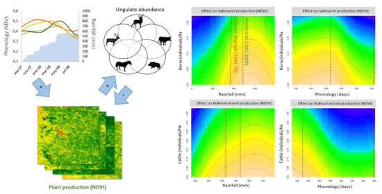
In this study we used a combination of remote sensing and in situ information to characterize the main factors driving the spatio-temporal variation in plant primary production, using the four main vegetation types of an iconic, Mediterranean protected area (Doñana National Park) hosting traditional ranching as a suitable case example. For this purpose, we analyzed its response to the two most important drivers: climatology (accumulated rainfall and vegetation phenology) and the grazing pressure exerted by wild (red and fallow deer) and domestic (cattle and horses) ungulates. In doing so, we sought to: (1) Quantify the separate and combined impact that the population densities of wild ungulates and the stocking rates of domestic herbivores have on the production of the different vegetation types. (2) Evaluate the resilience of the vegetation to the combination of environmental stress (strong inter-annual fluctuations in rainfall and phenology) and grazing pressure, and the expected impact of climate change thereupon. (3) Derive adaptive strategies enabling a sustainable combination of ranching and wildlife conservation in this type of area.
2. Materials and Methods
2.1. Study Area
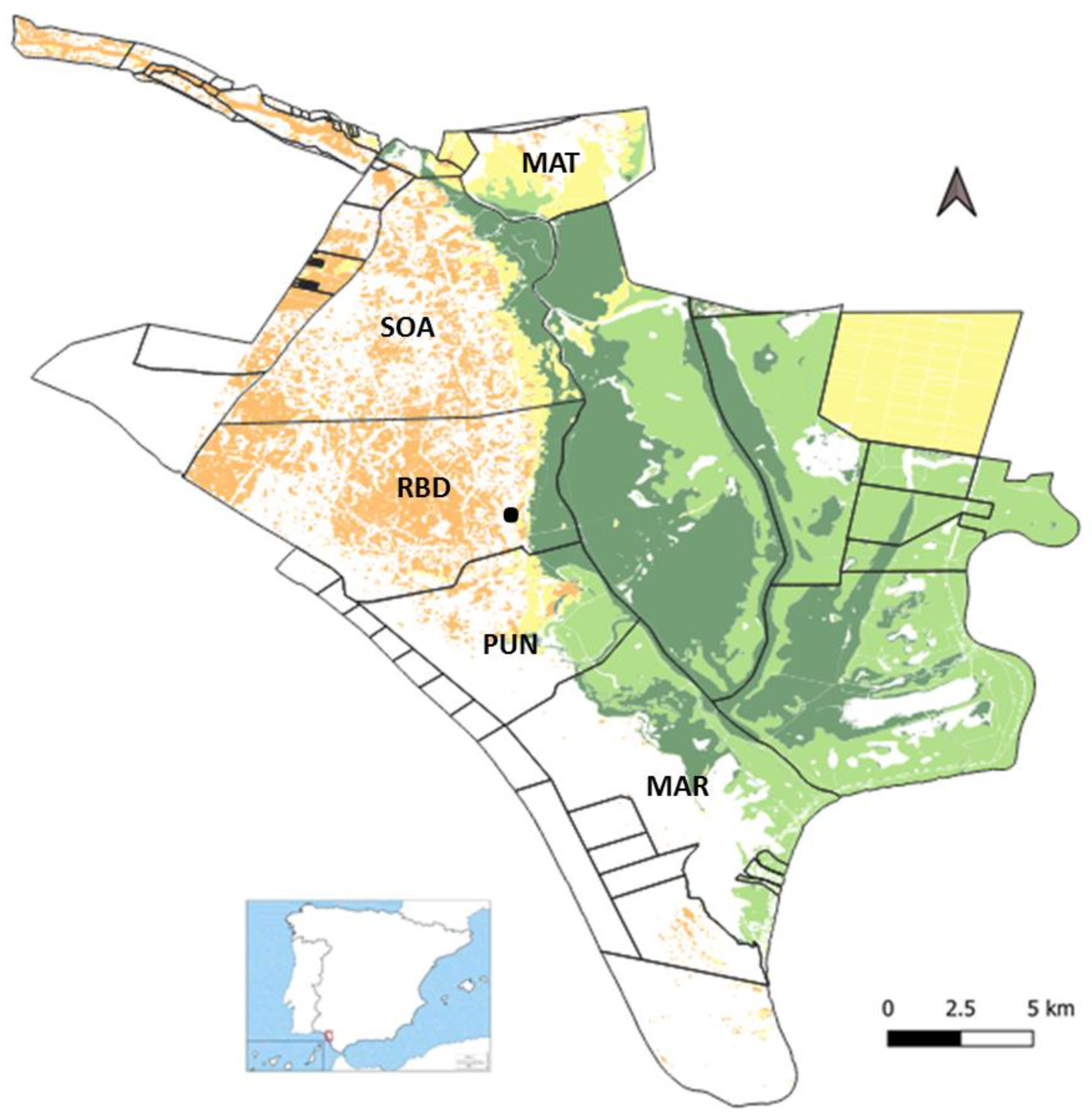
The research was carried out in the Doñana National Park (DNP onwards), a protected area located on the Atlantic coast of the southwest of the Iberian Peninsula. The region is characterized by a Mediterranean climate classified as dry sub-humid with marked seasonality. Doñana is characterized by high landscape heterogeneity. The inland areas have coastal formations and sand dunes almost free of vegetation; forests dominated by conifers (Pinus pinea and Juniperus phoenicea) and cork oaks (Querqus suber); and large shrub formations, grasslands, and wet shrub formations in the vicinity of lagoon systems, in the topographical depressions, and mainly at its border with the marsh, where it forms an ecotone in which soil moisture remains practically year-round. In the marshland, two main types of habitats can be differentiated: the saltmarsh, where the floods are not very prolonged, which is characterized by the presence of halophytes normally associated with certain levels of salinity in the soil (usually forming mosaics with grasslands); and the bulrush marsh, which can remain flooded for long periods each year and is characterized by extensive formations of plants of the family Cyperaceae.
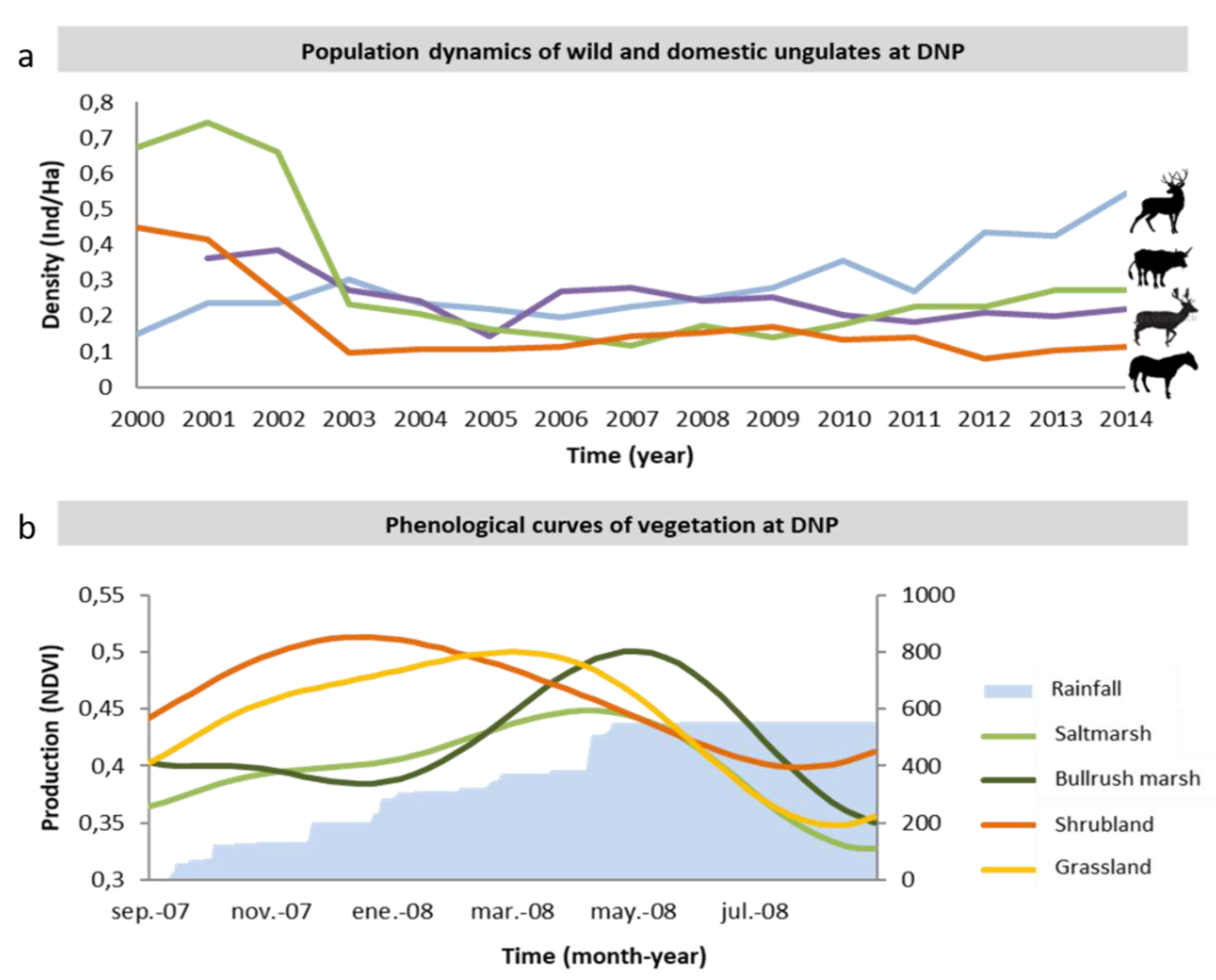
In the study area coexist populations of wild ungulates, red deer (Cervus elaphus) and fallow deer (Dama dama) and domestic ungulates (cattle and horses) that are traditionally bred in the different management areas of the National Park: Matasgordas (MAT), Los Sotos-Algaida (SOA), Biological Reserve of Doñana (RBD), El Puntal (PUN), and Las Marismillas (MAR). The density of the different species in the DNP (average density of the study period) is 6.26 red deer/km2, 6.01 cattle/km2 (excluding Matasgordas, where there is no presence of cattle), 3.89 fallow deer/km2, and 2.49 horses/km2 (excluding Matasgordas, where there is no presence of horses). Accounting for all herbivorous ungulates, the total density in the study area is 18.73 individuals/km2 (10.15 and 8.58 individuals/km2 for cervids and domestic livestock, respectively). The management areas are delimited by livestock-proof fences, limiting the movement of domestic ungulates within their own ranging area. Based on the average weight of the different ungulate species at the NPD (information provided by the National Park Office) the total biomass at the study area corresponding to these densities (average densities of the study period) are: 0.85 t/km2 for red deer, 0.20 t/km2 for fallow deer, 2.91 t/km2 for cattle, and 1.15 t/km2 for horses.
2.2. Delimitation of Vegetation Types
Our analysis focused on the four vegetation types accessible to wild and domestic ungulates (i.e., excluding forested stands such as stone pines, cork oaks, and coastal junipers) within the five National Park estates mentioned above. These were saltmarsh, bulrush marsh, shrubland, and grassland. The main vegetation types and their main characteristics are shown in
Table 1.
To define the different vegetation types, we selected the corresponding classes of vegetation maps (
Figure 1) elaborated in 2014 by the long-term monitoring program (PSPN; Andreu et al., 2014, pp. 37–59) [
41] of Doñana’s Singular Scientific-Technical Facility (ICTS-RBD), and grouped into the four types described above (
Figure 1). Subsequently, the polygons occupied by each of these types within each ungulate management unit (see below) were used to calculate their respective area and the variables derived from satellite-obtained NDVI values (see below). These tasks were performed with the ArcGIS 10.1 software [
42].
2.3. Estimation of Primary Production
Satellite information obtained from the Institute of Surveying, Remote Sensing and Land Information (IVFL) of the University of Natural Resources and Applied Life Sciences (BOKU), Vienna, was used to estimate the production of different vegetation types during the study period. This institution offers remote sensing products—smooth and continuous Normalized Difference Vegetation Index (NDVI) and Enhanced Vegetation Index (EVI)—from MODIS satellite images with different temporal resolution (from 16 to 7 days) from year 2000 to present. These products are the result of processing standard products from Terra and Aqua satellites, namely MODIS Level-3 16 day composite Vegetation Indices (VI) available at a spatial resolution of 250 m. The combination of 16 day composites from these two satellites—Terra (MOD13 series) and Aqua (MYD13 series)—allows acquisition of imagery at a temporal resolution of 7 days. Detailed information on the processes for creating these time series can be consulted in [
43] and at BOKU’s website (
https://boku.ac.at/rali/geomatics accessed on 10 January 2019).
In this study, we used the Normalized Difference Vegetation Index (NDVI), a commonly used vegetation index that serves as a proxy of vegetation density and plant health [
44]. NDVI was demonstrated to reflect appropriately the vegetation response to rainfall variability [
45] and extreme events (e.g., droughts) across different biomass around the world [
46]. We selected NDVI as a proxy of primary production because (1) we felt that it achieved the best balance between spatial resolution (pixel size) and robustness; and (2) we have already tested (i.e., calibrated and validated) a statistical model relating biomass production to NDVI for one of the main vegetation types [
47]. Alternative products, such as MODIS NPP and GPP, had a lower spatial resolution (1 to 0.5 km) than MODIS NDVI (0.25 km); and Landsat images, which provide a better spatial resolution (15–30 m) than MODIS, cannot be processed by the TIMESAT software (which requires regular time intervals) to fit the phenological curves, and showed large gaps due to different reasons, such as missing data (lines and columns), line shifts, radiometric incoherence, and the presence of clouds over the study area.
We took a number of precautions to address the limitations of using NDVI, as compared to NPP or GPP (which may work better in areas dominated by bare ground or with high tree cover) or Landsat (which provide better spatial resolution). First, the four vegetation types selected are structurally homogeneous and moderately productive, and we explicitly excluded forest stands with dense canopies and areas of bare soil. Second, we excluded from our dataset all pixels with mixed vegetation cover (i.e., those where the dominant vegetation occupied less than 70% of the pixel’s area).
We used the long-term series of NDVI values with the highest temporal resolution available (every 7 days) for the study period (January 2000–August 2014, corresponding to the period for which ungulate population data were available). For each vegetation type and within each management unit, we extracted the average NDVI value at each observation date (i.e., every 7 days) of the study period, using the Zonal Statistics function available in ArcGIS 10.1 [
42]. The Zonal Statistics tool calculates a defined statistic (e.g., the mean) for each zone defined by a dataset (e.g., land cover classes contained in a land cover map) based on the values of another dataset (a NDVI value raster dataset) resulting in a single output value for every zone in the input dataset (land cover classes). The resulting data series provided the phenological curves at each observation unit (
n = 75 per vegetation type, arising from a combination of 15 years × 5 management units). We then used the TIMESAT software [
48] to estimate the date and value of each annual NDVI peak, which we interpreted as surrogates of the vegetation’s phenology and production on each given growth period (referring, hereafter, to hydro-meteorological years, running from 1 September to 31 August). To filter the noise in the data we used the Savitzky–Golay filter fitting method and the default values for the remainder of settings in TIMESAT, namely: no spike method, one season per year, no adaptation to the upper envelope of the curve, and normal adaptation strength.
2.4. Rainfall
Rainfall data were also obtained from the database provided by Doñana’s Singular Scientific-Technical Facility (ICTS-RBD). This database provides long-term series of meteorological data collected at a meteorological station located inside the NPD (
Figure 1). We used daily rainfall data to calculate, on a daily basis, the cumulative rainfall throughout each hydrological year. From this series, we obtained the cumulative rainfall value at the day of the phenological peak of each vegetation type, separately for each management unit and each year. This value thus represents the cumulative rainfall at the moment at which given vegetation type reached its maximum annual production, at each management unit.
2.5. Ungulate Abundance
Data on the abundance of wild ungulates (red deer and fallow deer) at each management area were obtained from annual censuses conducted by the National Park service at the beginning of each annual reproductive (rutting) period, which differs approx. one month between the species (September for red deer and October for fallow deer). During rutting, individuals of both species concentrate on open areas, which greatly facilitates counting.
Population data on domestic ungulates were obtained from the National Park service, through censuses undertaken during the (bi)annual animal-health controls (June-September). These data only refer to adults older than 12 months, because young of the year were not reported consistently throughout the study period. National Park regulations set a cap at the total number of domestic ungulates allowed at each management area, which is adjusted on a yearly basis (see above). Hence, their (maximum) abundance is relatively independent of yearly fluctuations in environmental drives, and yearly values only show slight fluctuations relative to that year’s cap.
In the National Park, livestock is raised in a low-management ranching system where animals are only herded once or twice per year for the extraction of a portion of the individuals (most often young-of-the-year) and for health control. Wild ungulates are, in principle, unmanaged. Both groups are allowed to move and feed freely across the whole area of each management unit. Fences separating management units cannot be crossed by livestock (unless temporarily damaged), but they are relatively permeable for wild ungulates, which are able to cross them on a seasonal or even daily basis.
Based on this information, we built a database reflecting the abundances (number of adult individuals) of each of the four ungulate species at each management unit (
Figure 2). To correct for management unit size, we used these abundances to calculated population densities (number of individuals/ha). It is important to note that these values solely represent mean values per management unit: within each unit, the spatial distribution of the different species varies over space, across vegetation types, and over time. We limited our data to 2000–2014 because this is the time period for which consistent and reliable information on wild ungulate and livestock abundances was available.
2.6. Data Analysis
To analyze plant production (peak NDVI per unit area), we used hierarchical generalized additive models (HGAMs) fitted separately to each vegetation type, using the “GAM” function available in the R mgcv package [
49]. The models included production (peak NDVI) as response (dependent) variable; phenology (time of phenological peak, as number of days counted from 1 September), rainfall accumulated during the growth season (i.e., until the phenological peak), the interaction between phenology and rainfall, and the density (number of adults per unit area) of each of the four ungulate species, as independent, continuous covariates; and management areas as random factors. To account for temporal autocorrelation, we also included “year” as a continuous covariate. All models used a Gaussian error distribution and an identity link function. These models were subjected to automatic selection of covariates using the model argument “Select” [
50].
The predictor variable “phenology” (i.e., the day counted from the beginning of the hydrological year at which the phenological peak was observed in the NDVI curve) was taken to represent a surrogate of the evolution (i.e., the specific timing) of rainfall and temperature on that specific hydrological year. This variable was complemented with a second predictor variable, “accumulated rainfall” (i.e., the amount of rainfall accumulated until the moment at which the phenological peak took place), taken to represent a surrogate of the water resources available during that year’s specific growth period. Hence, the combination of these two variables represents the time and water resources available during the period that preceded the peak NDVI value used as the surrogate of plant production (i.e., as a response variable).
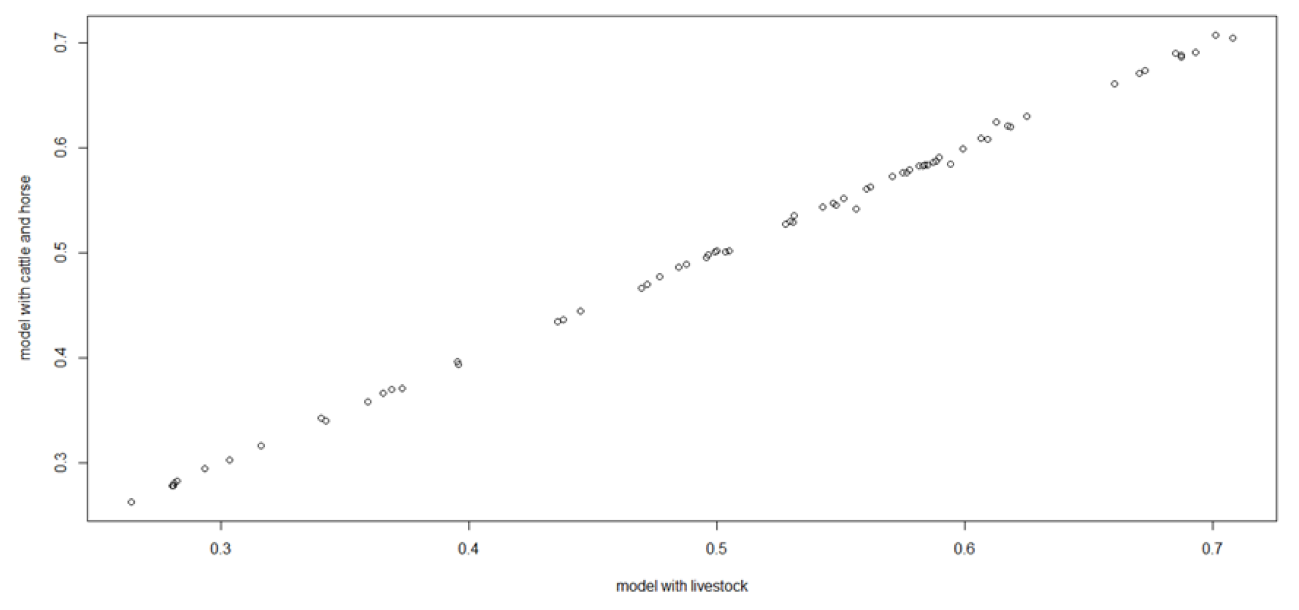
The different timing of the (wild and domestic) ungulate censuses vs. plant production estimates introduced a temporal uncertainty concerning which ungulate density values best reflect their impact on plant production. This uncertainty arises because plant production values reflect a biomass-accumulation process taking place from September to peak biomass, in late winter–spring (February–June); whereas ungulate density values during this period fall between measured values of the previous year (before the onset of the growth period) and those at the end of the growth period (June–September). Because all births and most deaths primarily take place during this period (during the summer, most animals are confined for animal-health control and artificially fed), we expected end-of-the-season density values to be more representative of ungulate impacts on vegetation than previous-season values. To objectively test for this assumption, however, we fitted separate models with either of the values, and selected the best-performing models based on the AIC score.
Residuals’ autocorrelation, if not adequately addressed, may result in biases in parameter estimates and tests of significance. Spatial autocorrelation was addressed by introducing the random factor “management unit”, which accounted for the spatial dependence of observations in both the dependent and independent variables. Temporal resolution was addressed by (1) including the covariate “year” in the model, and (2) computing estimates of the autocorrelation function of each model, using the Acf functions of R’s forecast package (Hyndman and Khandakar, 2007; Hyndman et al., 2020) [
51,
52]. These plots indicated that autocorrelation was adequately dealt with by the models, i.e., there was very low (and, in virtually all cases, non-significant) levels of residuals’ autocorrelation.
Finally, we used the function vis.gam in the mgcv package to produce contour plots of model predictions on primary production, for different combinations of ungulate abundance (only those with significant effects) and climatology (separate plots for rainfall and phenology). Based on these plots, we performed a visual comparison of historical data and climate change scenarios. These scenarios, represented by vertical lines in the prediction plots, showed the average values of accumulated rainfall or phenology (estimated separately for the average value of the other variable, respectively) as estimated from the historical series (1961–2000) and the MIROC RCP4.5 (2040–2070) regional-scale climatic change scenarios provided by Andalucia’s Environmental Information Network REDIAM at:
https://kerdoc.cica.es/cc?lr=lang_es# accessed on 20 October 2020 (REDIAM, 2014) [
53]. We chose the simulations based on the MIROC model for our study system, which tends to provide relatively drier estimates, because this model best reproduces the current climate in this area [
54] and best represents the interannual fluctuations in rainfall [
55]. Within it, we selected the RCP4.5 (or “mitigation”) scenario because it is based on a more realistic assumption of fossil fuel consumption (decreasing use of fossil fuels), thus providing a more conservative output than RCP8.5, which assumes a sustained fossil fuel use during the modelled time period [
56].
3. Results
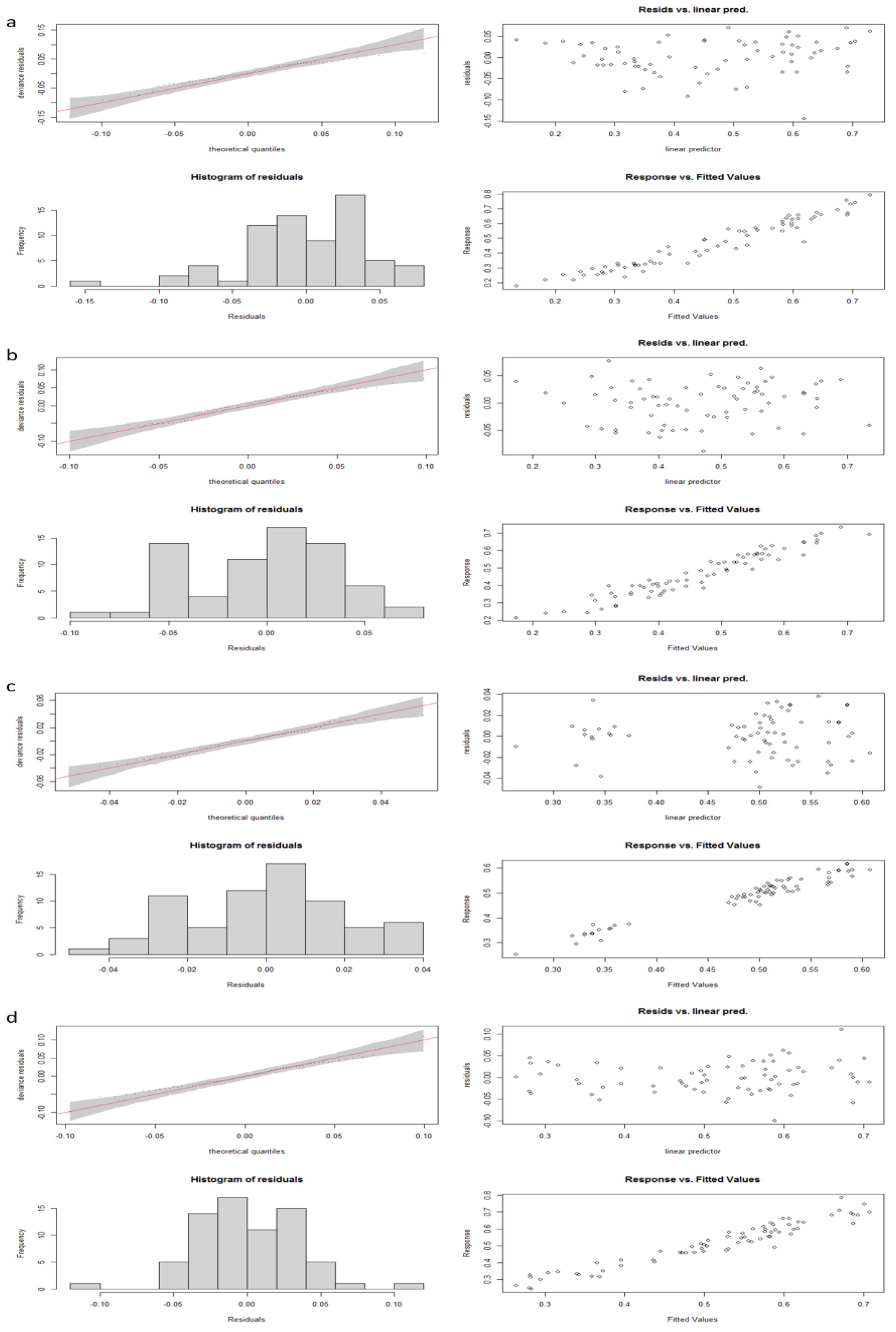
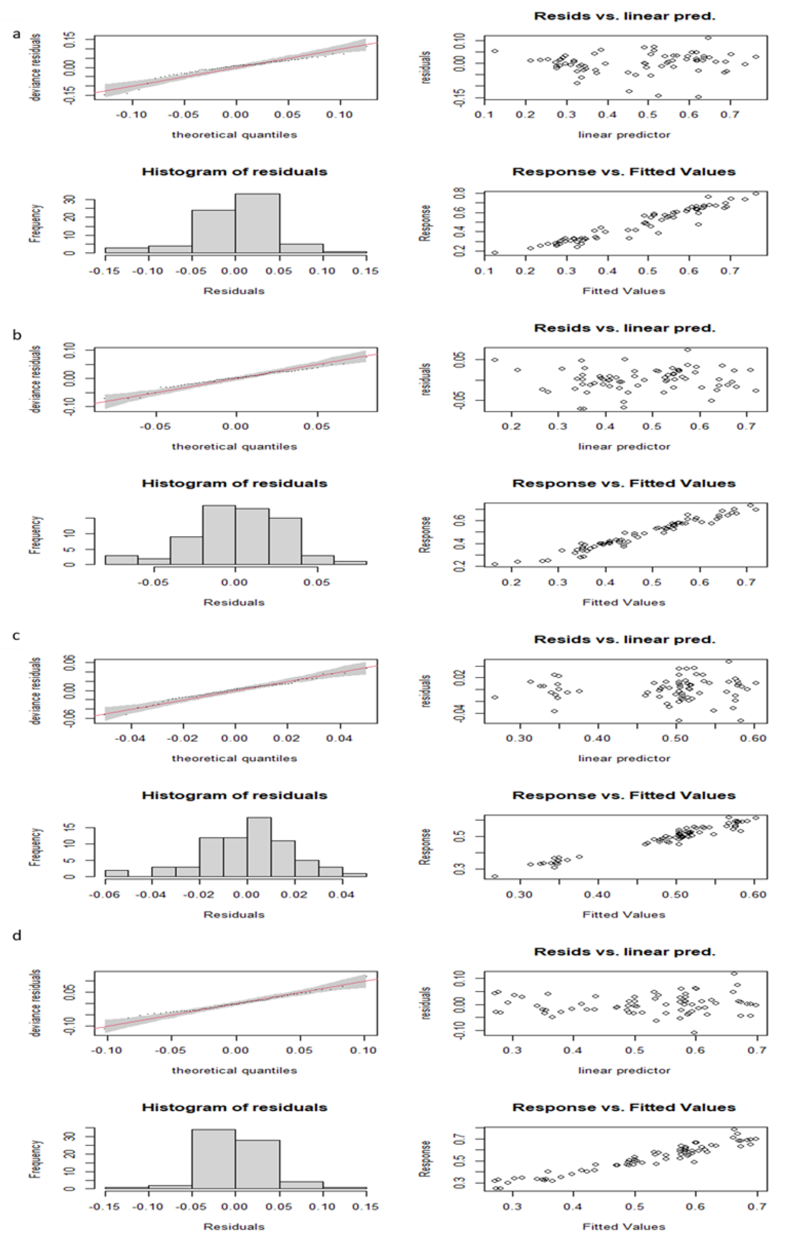
Models including end-of-the-season values of ungulate density performed systematically better than those including previous-season values (
Table 2). Hence, we only present here the results from the first type of model (although we also provide the results and diagnostic plots of the second type of models in
Table A1 and Figure A5,
Appendix A). All models well fitted the data (R
2 > 0.90, deviance explained > 92%;
Table 2) and fulfilled (or showed only slight departures from) the assumptions of residuals’ normality and homoscedasticity (
Figure A1,
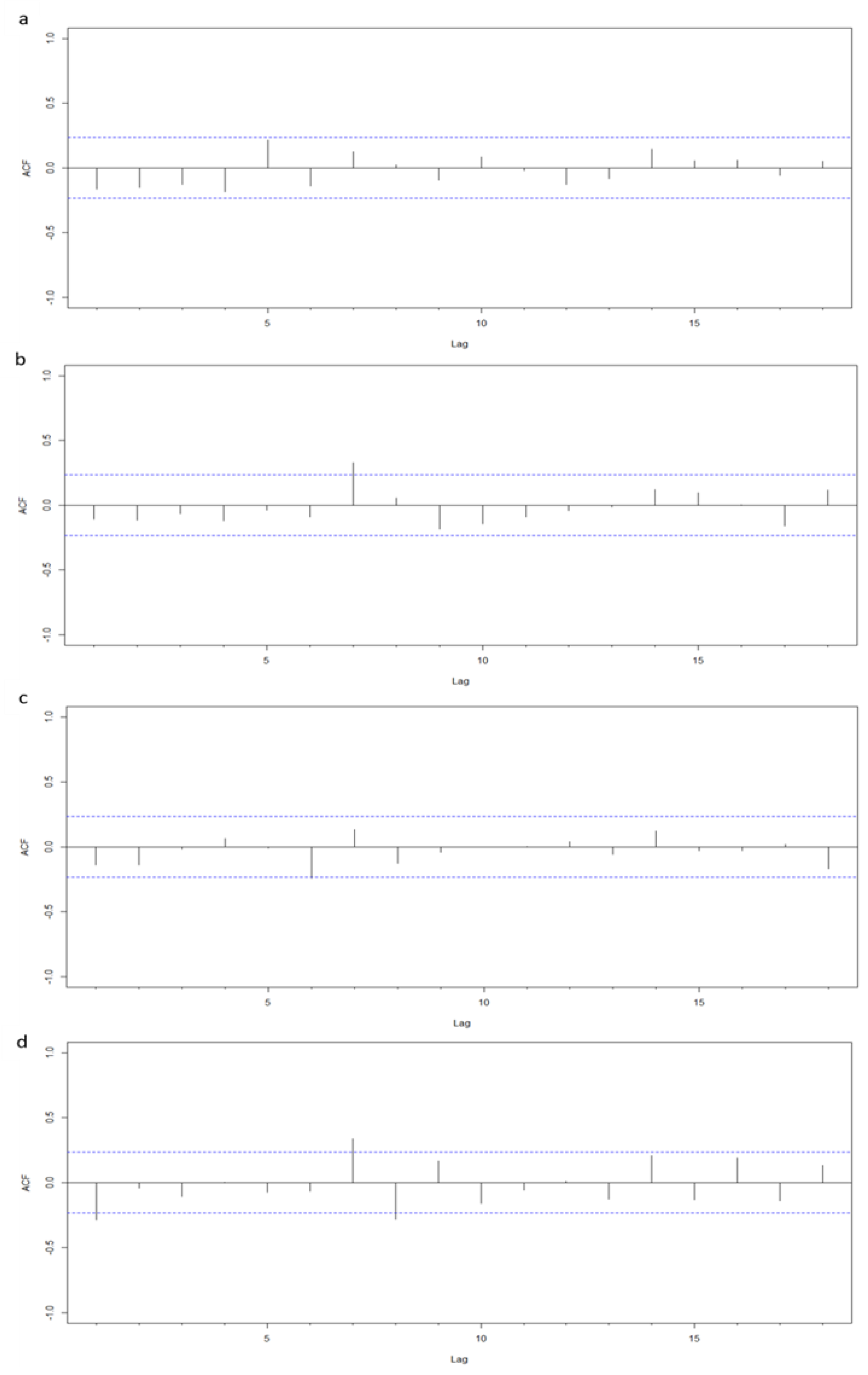
Appendix A). No model showed relevant signs of temporal autocorrelation (
Figure A2,
Appendix A).
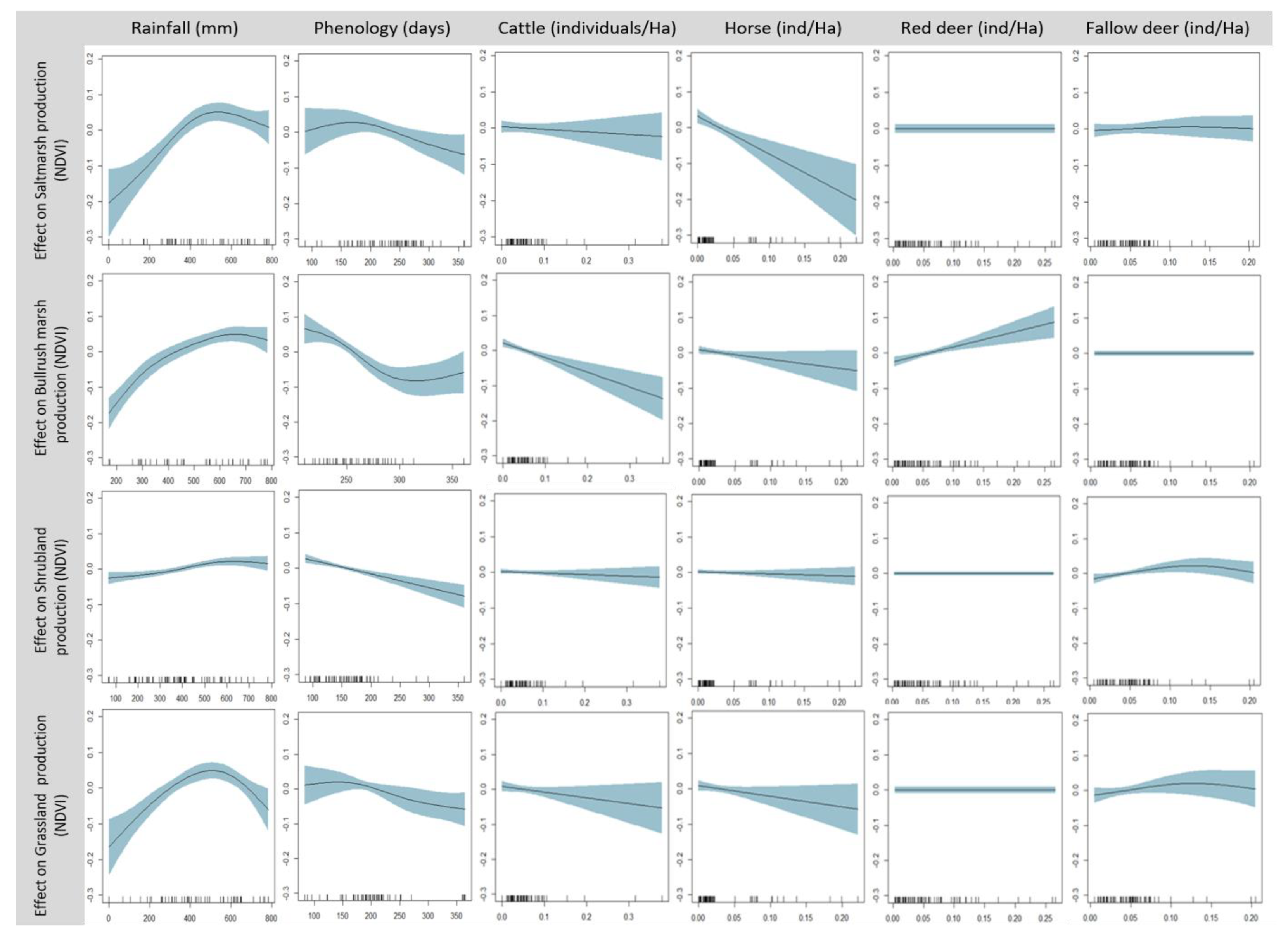
Variation in the length of the phenological cycle (days until NDVI peak) and the rainfall accumulated by then was significantly associated with the production of all four vegetation types. These effects were only additive (main factors significant, interaction not significant) for one vegetation type (shrubland) and synergistic (significant factors and interactions) for the other three (
Table 3). The two domestic ungulates differed strongly in their effects on different marsh vegetation types, which were always negative: saltmarsh production decreased significantly with horse density, bulrush marsh production decreased significantly with cattle density, and grassland production decreased significantly with both. Wild ungulate species had limited effects on vegetation production: red deer density was positively associated with bulrush marsh production, and fallow deer density showed a non-linear association with shrubland production.
The responses of the different vegetation types to rainfall showed a common pattern, i.e., an asymmetric, concave downward function, whose maximum was situated at medium or relatively high values of rainfall. However, the location of the maximum and the strength of the response (i.e., the slope of the upward and downward parts of the curve) varied strongly among vegetation types (
Figure 3). Saltmarsh production showed a pronounced increase at low rainfall levels, which started to saturate at ca. 400 mm, reached its maximum at 510 mm, and decreased moderately above it. Bulrush marsh production increased moderately at low rainfall, started to saturate around 600 mm, reached a maximum at 685 mm, and decreased slightly above it. Shrubland production showed a weak response, which increased slightly until reaching a maximum at 593 mm and decreased slightly after it. Grassland production showed a fairly symmetrical concavity that increased strongly until reaching a maximum at 511 mm and decreased strongly at higher levels of rainfall.
The association between the production of the different vegetation types and their phenology (time of phenological peak) also showed a common pattern, albeit with considerable differences in the intensity and shape of the response curve (
Figure 3). Responses range from a linear decrease in shrubland, to an inverted sigmoid curve in bulrush marsh, to asymmetric concave curves (with early peaks followed by a prolonged decrease) in saltmarsh and grassland. As a consequence, production peaks take place at the lowest phenology value registered (ca. days 87 and 210, respectively) in the shrubland and bulrush marsh, and close to day 150 for the saltmarsh and grassland. (These days correspond to early December, April, and February, respectively.)
The effect of rainfall and phenology was not merely additive (i.e., there was a significant interaction effect in the selected models) for three vegetation types: saltmarsh, bulrush marsh, and grassland (
Figure A3,
Appendix A). The interaction effects add to the separate effects of both variables showing (i) declines in production at both low rainfall + late phenology and high rainfall + early phenology, for saltmarsh; (ii) a decline in production at low rainfall + early phenology, but an increase at high rainfall + late phenology, for bulrush; and (iii) an additional decline in production at the lowest rainfall levels, which coincide with early phenologies, for grassland.
The density of domestic ungulates showed linear, negative effects on vegetation production (
Figure 3). Cattle density showed a strong effect on bulrush marsh production, a moderate effect on grassland production, and non-significant effects on saltmarsh and scrubland production. Horse density showed a strong effect on saltmarsh production, a moderate effect on grassland production, and not-significant effects on bulrush marsh and scrubland production.
The density of wild ungulates had either neutral or fairly weak effects on vegetation production (
Figure 3). Red deer density had non-significant effects on the production of three vegetation types (saltmarsh, scrubland, and grassland) and showed a linear, positive association with bulrush marsh production. Fallow deer density showed non-significant effects on saltmarsh, bulrush marsh, and grassland production, and non-linear effects (asymmetric concave curve peaking at a moderate density, ca. 0.13 adults/ha, and decreasing above it) on scrubland production. (Note that the relationship between shrubland production and fallow deer density is positive for most values included in the dataset, and the saturation and decrease in the curve only take place for four exceptionally high values included in it).
3.1. Combined Effect of Rainfall and Phenology
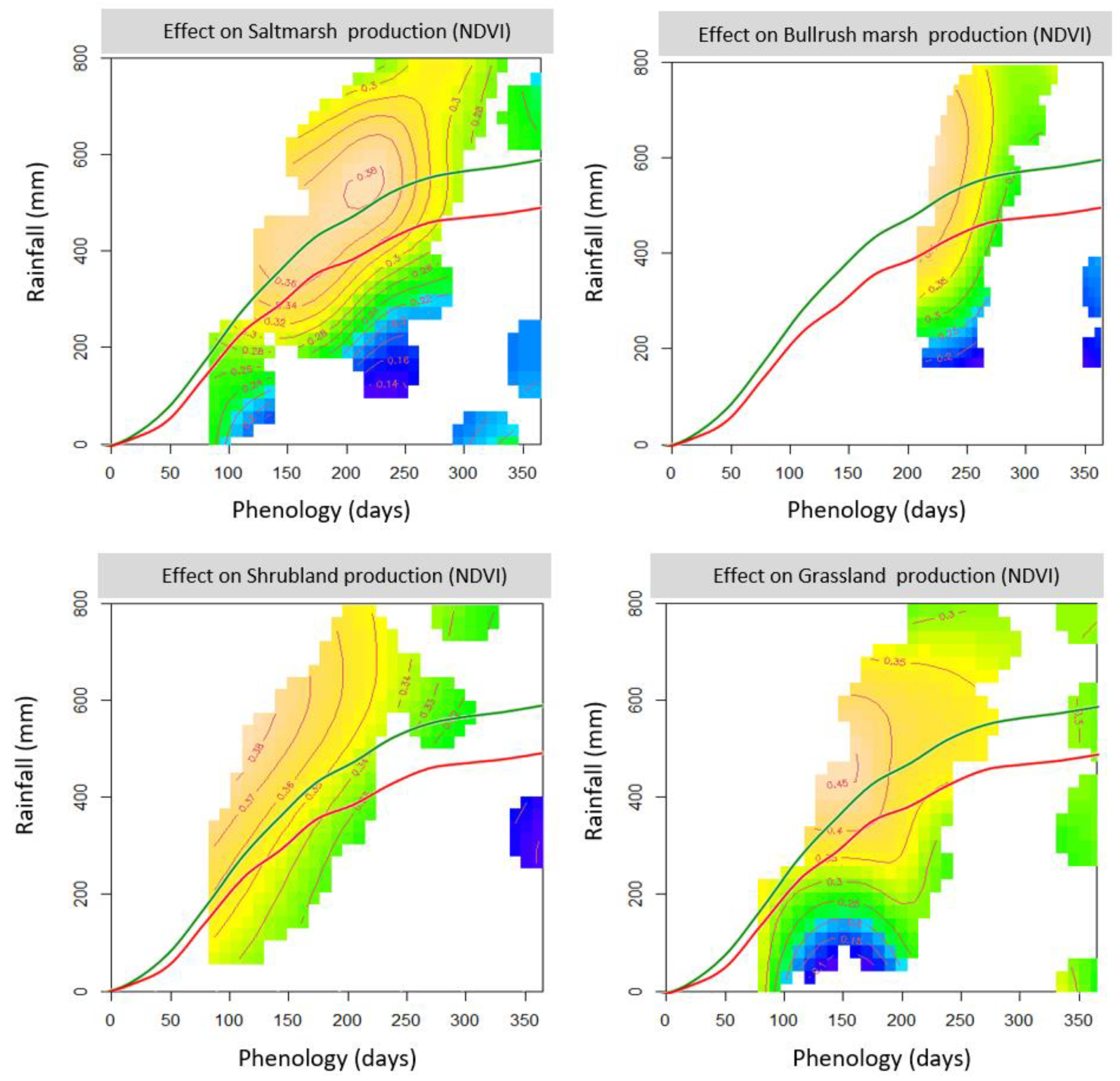
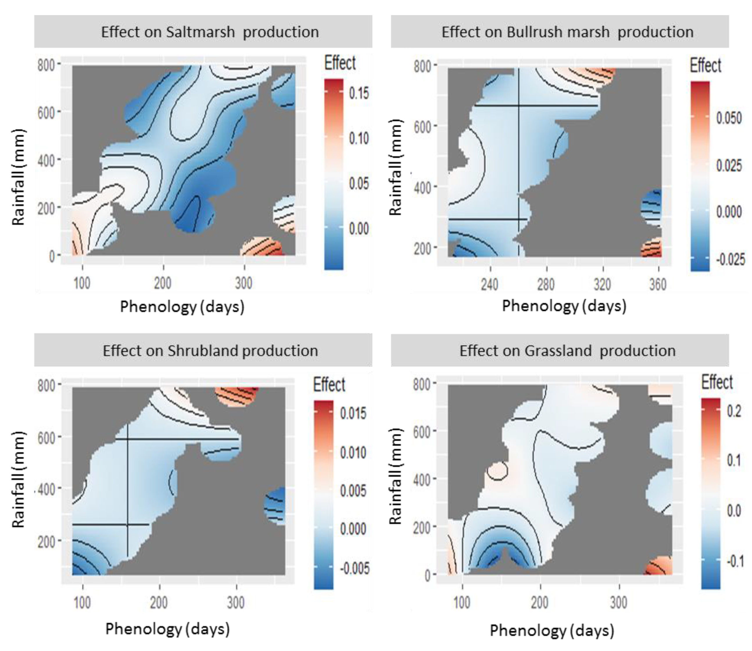
The non-linear relationships between production and both rainfall and phenology, and the positive association between the latter (which results in the absence of values at two types of combinations: early phenology with abundant rainfall, and late phenology with scarce rainfall) result in complex patterns that are best visualized using integrated interaction plots (
Figure 4). These plots show the combined effect of both variables (i.e., the sum of their main effects and their interaction) on the production of each of the four vegetation types; the variable ranges where no observations are available are left blank. These are particularly useful for defining the actual ranges of both variables for which optimal, suboptimal, and minimal production is predicted, which may differ considerably from those based on a direct extrapolation of the effect curves shown in
Figure 3.
The plots show a general pattern for the four vegetation types: production tends to follow a 2D concave downward function, with a local maximum at intermediate values of rainfall and phenology, and decreasing production below and above them. The location of this optimum and the shape of the curve (i.e., whether the decrease is rapid or slow, and more or less asymmetric) varies strongly among vegetation types. Saltmarsh production reaches its maximum when intermediate phenological peaks (days 200–240, i.e., early March–mid April) coincide with medium-high levels of accumulated rainfall (500–650 mm); then decreases strongly towards the lower part of the graph (i.e., at lower levels of rainfall, which take place at both early and intermediate phenologies); and decreases more gradually at higher rainfall levels (which coincide with delayed phenological peaks). Bulrush marsh production also peaks at medium-high levels of accumulated rainfall (500–650 mm) and early phenologies, which, due to the delayed growth cycle of this type of vegetation, take place relatively late in the season (days 200–250, i.e., late March–mid May); and decreases strongly towards the lower (low rainfall) and more moderately towards the upper-right (high rainfall and late phenology) parts of the graph. Shrubland production showed a flatter response, with peaks at medium-high levels of rainfall (450–550 mm) and early phenology (ca. day 120, i.e., early January, close to the earliest values recorded) and a smooth decrease at later phenologies, particularly in combination with increased rainfall. Grassland production peaked at intermediate levels of rainfall (420–440 mm) and early phenology (days 130–170 mm, i.e., early January–late February); and decreased strongly with decreasing rainfall, and decreased slightly for later phenologies and/or increased rainfall.
3.2. Model Predictions
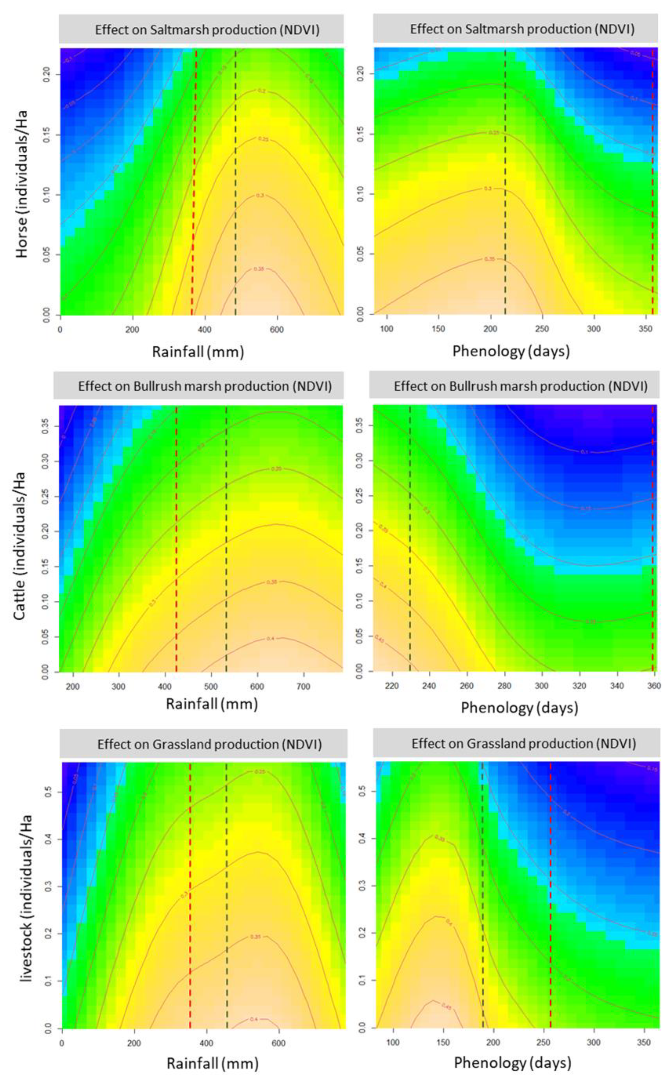
Plots of model predictions (
Figure 5) show the combined effect of either rainfall or phenology, and the grazing pressure exerted by domestic ungulate species, including only those with significant effects on each vegetation type: horses for saltmarsh, cattle for bulrush marsh, cattle and horses (combined as “livestock”) for grassland. (Shrubland is not included because there were no significant effects of domestic herbivores on it, and the effects of fallow deer were weak and dependent on 2–3 values of unusually high density). All plots show similar patterns: the decreases in primary production at lower rainfall levels or later phenological peaks are strongly accelerated at higher ungulate densities, reaching very low levels of plant production (<50% of the maximum), where they flatten out. Resilience to domestic ungulate grazing (showing as a vertical “crest” in the six panels) is relatively high at optimal rainfall and phenology. However, a displacement away from these conditions (both towards the left or the right part of the plots) causes production to drop as soon as moderate (0.1 cattle/ha for bulrush marsh, 0.2 livestock/ha for grassland) or even low (0.2 horses/ha for saltmarsh) densities of domestic ungulates are reached.
The prediction plots also show that the medium-term changes (2041–2070) in the quantity and temporal distribution of rainfall predicted by the MIROC RCP4.5 climate change scenarios (REDIAM, 2014) [
52] will probably cause a strong decrease in plant production, whose impact would be exacerbated at medium to high levels of livestock density. The effects of decreased rainfall levels are relatively moderate for the Doñana vegetation, albeit particularly strong for saltmarsh type. However, they will be compounded by the prolonged period required to achieve comparable levels of accumulated rainfall, i.e., by the strong delays in phenology required to attain them, whose strong impact on plant production will cause severe drops in plant productivity (NDVI < 0.15, i.e., <50% of maximum values) at intermediate levels of livestock density. Overall, the results indicate that the vegetation will face a combination of lower productivity and shorter phenological cycles, in turn causing lower biomass yields and shorter growth periods, and thus a strong decrease in food quantity and quality for herbivores.
4. Discussion
The use of remote sensing imagery combined with field surveys of ungulates and meteorological data provides a powerful tool to model the factors determining vegetation production at Doñana National Park. Model results indicate that the four different vegetation types differed in their phenology (time of the NDVI peak), their productivity (NDVI peak value), and their response to inter-annual changes in rainfall levels. These differences reflect the spatio-temporal segregation among vegetation types and may increase ecosystem resilience to both climatological variability and grazing. Regarding the latter, model results also show important differences in the impact of wild and domestic species on vegetation production: the former have neutral, weak unimodal, or even positive effects, whereas the later may have strong negative impacts on the production of most vegetation types (three of four: saltmarsh, bulrush marsh, and grassland). As a consequence, model prediction plots indicate that increasing livestock densities decreases vegetation resilience to decreased rainfall levels or delayed phenological peaks, thus exacerbating the impact of medium-term changes (2041–2070) in the quantity and temporal distribution of rainfall predicted by the climate change scenarios.
Our approach represents an attempt to simplify the modeling of plant production. We did not attempt to incorporate the whole suite of different meteorological factors (average, max. or min. temperature; length of the coldest period; temporal distribution of rainfall; etc.), and then discriminate at which lag levels they operate, because this would increase model complexity beyond its limit. Rather, we chose an indirect approach, in which two variables, “phenology” (the time of the NDVI peak) and “rainfall” (the amount of rainfall accumulated until such a moment) were introduced as surrogates for the integrated effect of climatology (the temporal sequence of rainfall and temperature) and water availability (from the start to the peak of the growth season) on plant production. The result was encouraging, because the fitted models, despite their relative simplicity (low number of parameters) were highly significant, explained a considerable proportion of the observed variation, and provided useful insight into the operation of the constituent variables, including the effects of ungulate grazing. Detailed modeling of the ultimate, climatological causes of these effects, using a more extensive dataset, will however be necessary to derive more precise predictions and forecasts.
Three of the four vegetation types reached their maximum production at or close to the average rainfall levels of the historical series (ca. 500 mm), albeit marshland vegetation performed better at higher rainfall levels (ca. 600 mm) and one type (grassland) did so at lower rainfall levels (ca. 400 mm). This convergence around average rainfall probably reflects the adaptation of the vegetation to local climate conditions, on which differences following the gradient of hygrophily (from the more xerophilous shrubland to the seasonally mesophylous bulrush marsh) is superimposed. In addition, model results reflected the considerable phenological differences among the different vegetation types. These differences result in a complex spatio-temporal pattern of plant primary production, in which the spatial mosaic of vegetation types is associated with seasonal differences in plant production that, in turn, vary among years. This allows for considerable resilience to variations in rainfall level and temporal distribution, given that these fluctuations do not undergo extreme departures from average levels. Rainfall levels ensuring optimal production for one vegetation type will result in suboptimal production for the other types, and vice-versa; conversely, the temporal sequence of production peaks along the xeric-mesic gradient will buffer the loss of production of any given vegetation type through the aforementioned increase in the production of other vegetation types, which not only increases the peak but also expands the breath of the phenological curves. Hence, ensuring a balanced access to the different vegetation types may hold the key to ensuring the supply of a diverse set of forage resources to meet the herbivore guild’s dietary needs [
57], thus extending the availability of resources for herbivores, facilitating the maintenance of biodiversity patterns and processes [
58], and increasing its resilience to climatic conditions predicted by climate change scenarios [
59]. This may require, however, a wise choice of stocking rates, tailored to the productivity offered by each vegetation type, in particular, the most limiting type at each management unit (see below).
Model results also indicated that the impact of ungulate density (i.e., grazing pressure) on plant production differed strongly between wild and domestic species. These distinct effects may, at least partially, arise from the strong difference in stocking rates when expressed in terms of animal biomass. Although population densities were comparable among the four different herbivores (averaging 10.15 and 8.58 individuals/km
2 for wild and domestic ungulates, respectively), the body mass of cattle and horse is four- to six-fold higher than the body mass of the two cervid species present in the study area, thus resulting in much larger biomass stocking rates of domestic ungulates (1.05 t/km
2 of cervids vs. 4.06 t/km
2 of livestock). However, this does not seem to be the only reason behind this discrepancy because linear, negative effects of both cattle and horses on vegetation were also exerted at low densities (i.e., if responses were comparable to those found for wild ungulates, non-linear effects with flat responses at low densities would be expected). Differences in foraging intensity, diet choice, and behavior (including the proportion of non-consumptive plant damage, e.g., by trampling in soft soil) probably combine with higher consumptive rates (related to the larger body mass) to cause the negative impact of domestic, but not wild, herbivores on vegetation. The positive effects of wild ungulates on several vegetation types (either at all densities, or at the low-density part of the concave downward curves) may result from facilitation mechanisms, e.g., eliminating shading by less productive plant parts, removing apical dominance, and favoring regrowth; [
60,
61] or may simply reflect indirect, non-causal effects (e.g., displacement away from areas grazed by herbivores with more severe impacts).
Among the domestic herbivores, cattle and horses showed similar effects (i.e., linear negative responses of similar slope) but affecting different vegetation types, probably indicating a trophic niche segregation between these two species. Both species caused similar, moderately negative effects on the grassland, the most suitable type of pasture for them. However, cattle showed strong negative effects on bulrush marsh vegetation, whereas horses did so for the saltmarsh vegetation. Preliminary data on habitat use and knowledge shared by local ranchers suggest that this difference may reflect different foraging choices by these two herbivores, with cattle being able to extensively exploit the bulrush marsh and horses feeding primarily in saltmarsh vegetation (both before bulrush emergence and after a few weeks of growth, when bulrush plants become unpalatable). Future work characterizing these preferences in detail, e.g., through the use of GPS collars, will be of key importance to adequately calculate stocking rates of the different herbivores, adjusting them to the type of vegetation exploited, and optimizing the design and operation of management (thus, foraging) units.
The resilience of the vegetation to the combination of environmental stress (strong inter-annual fluctuations in rainfall and phenology) and grazing pressure will be further compounded by the expected impact of climate change. According to the model predictions, increasing livestock densities will decrease vegetation resilience to decreased rainfall levels or delayed phenological peaks, thus exacerbating the impact of medium-term changes (2041–2070) in the quantity and temporal distribution of rainfall predicted by the climate change scenarios. Based on the predictions of a moderate scenario of the MIROC model, we may conclude that the END’s vegetation will face increasingly constraining conditions for its development. Vegetation will face a 16.5% decrease in annual rainfall. This shortage is not homogeneous over time; hence, its effect is compounded by its temporal interaction with vegetation phenology. If vegetation maintains its current patterns of phenological development, most types (all but the shrubland) will face a larger decrease (17.8–18.8%) during the growth period; and, if it adjusts its development to the changes in rainfall distribution, its phenological peak will have to be significantly delayed to achieve the levels of rainfall at which their production peaks (ca. 60 days for grassland vegetation,
Figure 4). Else, they will not be able to achieve these levels because the potential growth season will end, prior to the commencement of the period of prolonged summer drought (saltmarsh and bulrush marsh vegetation,
Figure 4). The latter trend is particularly concerning because the delay in phenology necessary to achieve optimal rainfall will play against the general trend resulting from the concomitant increase in temperatures, i.e., an acceleration in vegetation phenology. Indeed, the observed phenological shift of vegetation in the Northern Hemisphere during recent decades reflects an advance of 0–12 days [
62,
63,
64], which would result in even lower levels of accumulated rainfall for the END’s vegetation.
The moderate reduction in primary production caused by these changes in rainfall amount and patterns, especially in marshland vegetation (9–20% for the two upper panels of
Figure 4), will become significantly stronger under a scenario of moderate to high herbivore pressure, which can be expected under current densities of domestic herbivores (e.g., 11–28% for densities of 0.15 individuals/ha in the two upper panels of
Figure 4). The effect of moderate herbivore density is smaller in grassland vegetation, but accelerates strongly at higher densities (lowest panel,
Figure 4). The overall result is a strong decrease in the resilience of vegetation production to climate change in the presence of moderate to high domestic herbivore pressure. These effects will have, in turn, major consequences on the secondary production of livestock, whose profitability and sustainability will be thus compromised [
65,
66]. These results highlight the importance of considering local stressors in combination with predicted climatic conditions in order to better understand the complex evolution of specific habitats.


