An Endmember Bundle Extraction Method Based on Multiscale Sampling to Address Spectral Variability for Hyperspectral Unmixing

Abstract

With the improvement of spatial resolution of hyperspectral remote sensing images, the influence of spectral variability is gradually appearing in hyperspectral unmixing. The shortcomings of endmember extraction methods using a single spectrum to represent one type of material are revealed. To address spectral variability for hyperspectral unmixing, a multiscale resampling endmember bundle extraction (MSREBE) method is proposed in this paper. There are four steps in the proposed endmember bundle extraction method: (1) boundary detection; (2) sub-images in multiscale generation; (3) endmember extraction from each sub-image; (4) stepwise most similar collection (SMSC) clustering. The SMSC clustering method is aimed at solving the problem in determining which endmember bundle the extracted endmembers belong to. Experiments carried on both a simulated dataset and real hyperspectral datasets show that the endmembers extracted by the proposed method are superior to those extracted by the compared methods, and the optimal results in abundance estimation are maintained.

1. Introduction

Hyperspectral images have been widely used in various fields such as classification [1,2,3], target detection [4,5], and quantitative inversion [6,7,8] due to the narrow continuous spectral bands [9] which can provide a large amount of spectral information for each pixel. No matter the spatial resolution, mixed pixels are always widely encountered in remote sensing images which is always the main reason for the limitation to the accuracy of traditional remote-sensing applications at a pixel level. To improve the precision of remote sensing applications, the problem of mixed pixels must be solved. The main task of unmixing is to decompose the mixed pixels into pure materials (called endmembers) and their corresponding proportions (called abundance).

At present, the common methods for endmember extraction are based on using a spectrum to represent one class of material. The main methods are divided into two categories: (1) when there are pure pixels in the image, the main idea of endmember extraction is to search some pixels that can form a convex simplex with maximum volume or have the largest projections in some vectors. Representative algorithms include pixel purity index (PPI) [10], N-FINDR [11], vertex component analysis (VCA) [12], orthogonal subspace projection (OSP) [13], etc.; (2) when the image does not contain pure pixels, the relative algorithms aim to seek a convex simplex with a minimum volume that contains all the pixel points. Methods in this category include iterative-constrained endmembers (ICE) [14], minimum volume-constrained nonnegative matrix factorization (MVC-NMF) [15], and minimum volume simplex analysis (MVSA) [16]. However, with the improvement of spatial resolution of remote sensing images, the phenomenon of spectral variability caused by various factors including acquisition environment [17], illumination [18] and materials per se [19] in hyperspectral images becomes more and more severe, especially in some scenes where various features are more concentrated, such as wetlands and forests. In this case, a single spectrum is insufficient to represent one class of features. Therefore, most aforementioned extraction methods above are not applicable to hyperspectral images with high spectral variability. Previous studies [20,21] have indicated that the above methods which ignore spectral variability can potentially lead to poor estimates of abundances.

Multiple endmember spectral mixture analysis (MESMA) [22] was proposed in order to solve the problem of spectral variability. MESMA, however, requires not only a known spectral library but also substantial computing costs when many spectra need to be tested. In addition, some scholars have proposed methods to address spectral variability without a known spectral library, including parametric endmember models [23,24], Bayesian methods [25,26], and endmember bundle extraction methods. Among them, parametric models and the Bayesian methods require a large number of parameters to be set [27]. However, endmember bundle extraction methods can basically make up for the above shortcomings. The concept of “bundle” [28] means that the endmembers of each feature are represented by a collection containing multiple spectra. Many algorithms [29,30,31,32,33] for endmember bundle extraction have been proposed. Among them, many methods extract endmembers from each subregion of the original image, and then cluster the extracted endmembers to obtain endmember bundles. However, the above experiment processes may extract mixed pixels as candidate endmembers when the subregion contains no pure pixels. To address these issues, scholars adopted PPI [34] and a homogeneity index (HI) [35] to ensure the purity of candidate endmembers. At present, endmember bundle extraction is still in its infancy, and the development of this field still needs additional research.

Compared with endmember extraction methods, endmember bundle extraction methods require an additional step of clustering to group the extracted endmembers. Currently, most endmember bundle extraction algorithms group extracted endmembers [30,35] using the K-means clustering method. Then, the clustering results are compared with ground truth as a priori knowledge to identify which material each endmember bundle belongs to. K-means clustering has a better performance in the datasets with more interclass variability than intraclass variability. However, due to the spectral variability, K-means clustering struggles to accurately complete the clustering of a large number of endmembers.

To further improve the accuracy of hyperspectral unmixing, it is necessary to develop a new method to address the above problems. The main contributions of this paper are as follows: (1) in order to address the spectral variability of hyperspectral images, a multiscale resampling endmember bundle extraction (MSREBE) algorithm is proposed in this paper. Candidate endmembers are extracted from sections of each sub-image generated from the original image at different sampling scales. Pure pixels, which are selected as candidate endmembers at multiple sampling scales, are optioned as endmembers. Afterward, the endmembers are clustered into endmember bundles for each material; (2) the stepwise most similar collection (SMSC) clustering method is proposed in this paper. The extracted endmembers are clustered with their most similar endmembers step by step according to prior knowledge. SMSC partitions the spectral variability of all extracted endmembers at each step, which can reduce the influence of spectral variability in the clustering.

The remainder of this paper is organized as follows: Section 2 describes four state-of-the-art algorithms which are compared with the proposed algorithm. The proposed algorithm is presented in Section 3. Section 4 displays four experiments with both a simulated dataset and real hyperspectral datasets, as well as discusses the results obtained from the experiments. Section 5 concludes this paper.

2. Relative Research Works

In this section, four typical algorithms, namely, VCA, image-based endmember bundle extraction (EBE), spatial and spectral feature-based EBE (SSEBE) and archetypal analysis EBE (AAEBE), are introduced. These methods are taken for comparison when conducting experiments on both a synthetic dataset and real datasets.

2.1. VCA

VCA is a typical endmember extraction algorithm based on convex geometry theory [12]; the main idea of this method is that projection of the data cloud formed on the hyperplane is a convex simplex whose vertices are endmembers. By projecting all pixels onto a random vector, the first endmember is the pixel with the largest projection. Then, the remaining endmembers are iteratively extracted by projecting the remaining pixels onto the orthogonal direction of the subspace, which is composed of the extracted endmembers. The pixel corresponding to the limit projection is taken as the next endmember. Suppose the collection composed by extracted endmembers is expressed as ${\left\{{\mathrm{e}}_{\mathrm{j}}\right\}}_{\mathrm{j}=1}^{\mathrm{k}}$ and the corresponding matrix is described as E_k. Then, the (k + 1)-th endmember ${\mathrm{e}}_{\mathrm{k}+1}$ can be extracted via Equation (1).

$${\mathrm{e}}_{\mathrm{k}+1}=\arg \underset{{\mathrm{r}}_{\mathrm{i}},\mathrm{i}=1,\dots ,\mathrm{n}}{\max }\left\{\left|{\mathrm{w}}_{\mathrm{k}}^{\perp }{\mathrm{r}}_{\mathrm{i}}\right|\right\},$$

(1)

where ${\mathrm{r}}_{\mathrm{i}}$ represents the remaining pixels, and ${\mathrm{w}}_{\mathrm{k}}^{\perp }$ is one random vector of ${\mathrm{E}}_{\mathrm{k}}^{\perp }$, which is calculated via Equation (2).

$${\mathrm{w}}_{\mathrm{k}}^{\perp }=\frac{{\mathrm{E}}_{\mathrm{k}}^{\perp }\mathsf{\xi }}{{\Vert {\mathrm{E}}_{\mathrm{k}}^{\perp }\mathsf{\xi }\Vert }_2},$$

(2)

where $\mathsf{\xi }$ is an independent identically distributed zero mean Gaussian vector, i.e., $\mathsf{\xi }~\mathrm{N}\left({0,\mathrm{I}}_{\mathrm{k}}\right)$. ${\mathrm{E}}_{\mathrm{k}}^{\perp }$ is the orthogonal projection matrix of E_k, which is calculated via Equation (3).

$${\mathrm{E}}_{\mathrm{k}}^{\perp }{=\mathrm{I}}_{\mathrm{k}}{-\mathrm{E}}_{\mathrm{k}}{{(\mathrm{E}}_{\mathrm{k}}^{\mathrm{T}}{\mathrm{E}}_{\mathrm{k}})}^{-1}{\mathrm{E}}_{\mathrm{k}}^{\mathrm{T}}.$$

(3)

2.2. EBE

The principle behind EBE is to carry out an endmember extraction algorithm in every subset [30]. The specific process is as follows: subsets are generated by sampling randomly using the pixels from the original hyperspectral images. The main assumption for adopting this random strategy in the selection of pixels is that a smaller proportion of image pixels can be used to approximate the statistics of the original image. That is, if there are numerous pure pixels for each endmember in the scene, the image subsets generated by random sampling will also have pure pixels. Then, pure pixels in each subset can be extracted by the endmember extraction methods. Subsequently, the spectral set will consist of spectral signatures from different features after all subsets are analyzed. Finally, the spectral set can be clustered into some categories corresponding to each ground component by K-means clustering with the Euclidean distance as a similarity measure. K as prior knowledge in this clustering method represents the number of clustering collections, which is determined on the basis of specific experimental needs.

2.3. SSEBE

SSEBE is proposed to extract endmember bundles using both spatial and spectral information [35]. The steps of this method are as follows: (1) to reduce the computational complexity, the PPI algorithm is used for coarse screening of original hyperspectral images. All pixels of hyperspectral image are projected onto multitude skewers. When the frequency of a pixel appearing as the maximum or the minimum of projections is more than the given threshold, the pixel is considered as a candidate endmember; (2) according to the idea that pure pixels generally locate in spatially homogeneous areas, SSEBE calculates HI, which is the index to determine whether the pixels are in a homogeneous region, between each pixel and its adjacent pixels, with spectral information divergence (SID) as a measure. A smaller HI of the pixel denotes greater similarity to its adjacent pixel and a greater likelihood of being in the homogeneous region; (3) the HI threshold of every subregion is determined by adaptively adjusting according to the proportion of the selected candidate endmembers. The principle of setting the threshold is that the percentage of candidate endmembers is no more than 2–5% of the whole data set. Then, candidate endmembers whose HI are smaller than threshold are selected to make up the spectral set; (4) the spectral set is clustered using the K-means clustering method, with the initial clustering centers obtained by OSP.

2.4. AAEBE

AAEBE was firstly applied for archetypal analysis and was originally designed for machine learning problems to endmember bundle extraction [34]. This method considers the similarity of intra-endmembers and represents each endmember by a few typical spectra to reduce computation for unmixing. The main process of the method is as follows: (1) similarly to the first step in SSEBE, PPI is used to extract candidate endmembers; (2) archetypal analysis is used to extract the first-level endmembers among the candidate endmembers extracted from step (1); (3) the candidate endmembers are clustered into several collections on the basis of the first-level endmembers, and then a second archetypal analysis is used in turn in each collection to obtain pure pixels of each endmember. After all the above steps, the endmember bundles corresponding to each material are extracted.

3. Multiscale Resampling Endmember Bundle Extraction (MSREBE)

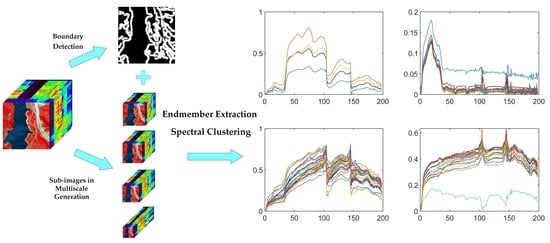
The proposed method consists of four steps: (1) boundary detection, (2) sub-images in multiscale generation, (3) endmember extraction from each sub-image, and (4) stepwise most similar collection clustering. A brief illustration of the method is shown in Figure 1.

3.1. Boundary Detection

The pixels in the hyperspectral image can be divided into pure pixels and mixed pixels. Mixed pixels contain the spectral information of multiple materials. The boundary pixels usually occur at the intersection of two or more features, which are more likely to be mixed pixels. In order to reduce the probability that mixed pixels are selected as endmembers, boundary pixels and their four neighborhood pixels are deleted before extracting endmembers.

The first principal component obtained from the hyperspectral image according to principal component analysis (PCA) [36] contains the primary information of hyperspectral images. In this paper, the boundary pixels are detected on the basis of the first principal component of the hyperspectral image. The canny edge detector, a classical edge detection operator [37], is used to detect the boundary. This step consists of two operations: (1) carry out PCA of the hyperspectral image and obtain the first principal component; (2) use the canny detector to identify boundary pixels of the first principal component and label the location of boundary pixels and their four neighborhood pixels.

3.2. Sub-Images in Multiscale Generation

It is difficult to extract endmember bundles from a hyperspectral image with high spectral variability. In this paper, we extracted endmembers in sub-images with relatively low spectral variability generated by sampling original hyperspectral image. The adjacent pixels in the original image were assigned to different sub-images. Figure 2 shows the generation process of sub-images at a sampling scale of 2. According to the above operation, sub-images have similar feature distributions to the original image with lower spectral variability.

The spectral variability cannot be significantly reduced when the sampling scale is small. On the contrary, there may be no pure pixels in sub-images when the scale is too large. Therefore, the best sampling scale is difficult to determine. Under this condition, we extracted candidate endmembers at multiple scales, ensuring that candidate endmembers could adequately show the spectral variability of the original image. We firstly set 1, 2, 3, and 4 as the sampling scales considering some images of a small size. Then, the maximum sampling scale was determined via Equation (4) concluded from multiple experiments.

$$\mathrm{MAX\_scale}=\min (\mathrm{M}/20,\mathrm{N}/20),$$

(4)

where M and N represent the number of rows and columns of the original hyperspectral image, respectively. To reduce the computational burden, we adopted the method of exponential growth to calculate the remaining sampling scales.

3.3. Endmember Extraction from Each Sub-Image

After the above step, the spectral variability among different regions still exists because the feature distributions of sub-images are similar to the original image. If endmembers are extracted directly from sub-images, the final extracted endmembers will be in a gathering state. That is, extracting endmembers in sub-images with similar spatial structures may lead to the situation that the extracted endmembers are located in similar positions of the sub-images. When the extracted pure pixels are mapped onto the original image, pure pixels of the endmember may appear in close areas to form a gathering state. To solve the above problems, sub-images generated at the same sampling scale were alternately divided into four sections in the horizontal and vertical directions. Then, candidate endmembers were extracted from each section with VCA after deleting the boundary pixels detected in step 3.1. Following the above steps, some pixels were extracted as candidate endmembers at multiple sampling scales. When a pixel is selected as an endmember in more sub-images, the probability of the pixel being a pure pixel as the endmember is higher. To select more representative endmembers, a threshold T is required for screening candidate endmembers; in this paper, one-third of the sampling scale number was adopted as the threshold T.

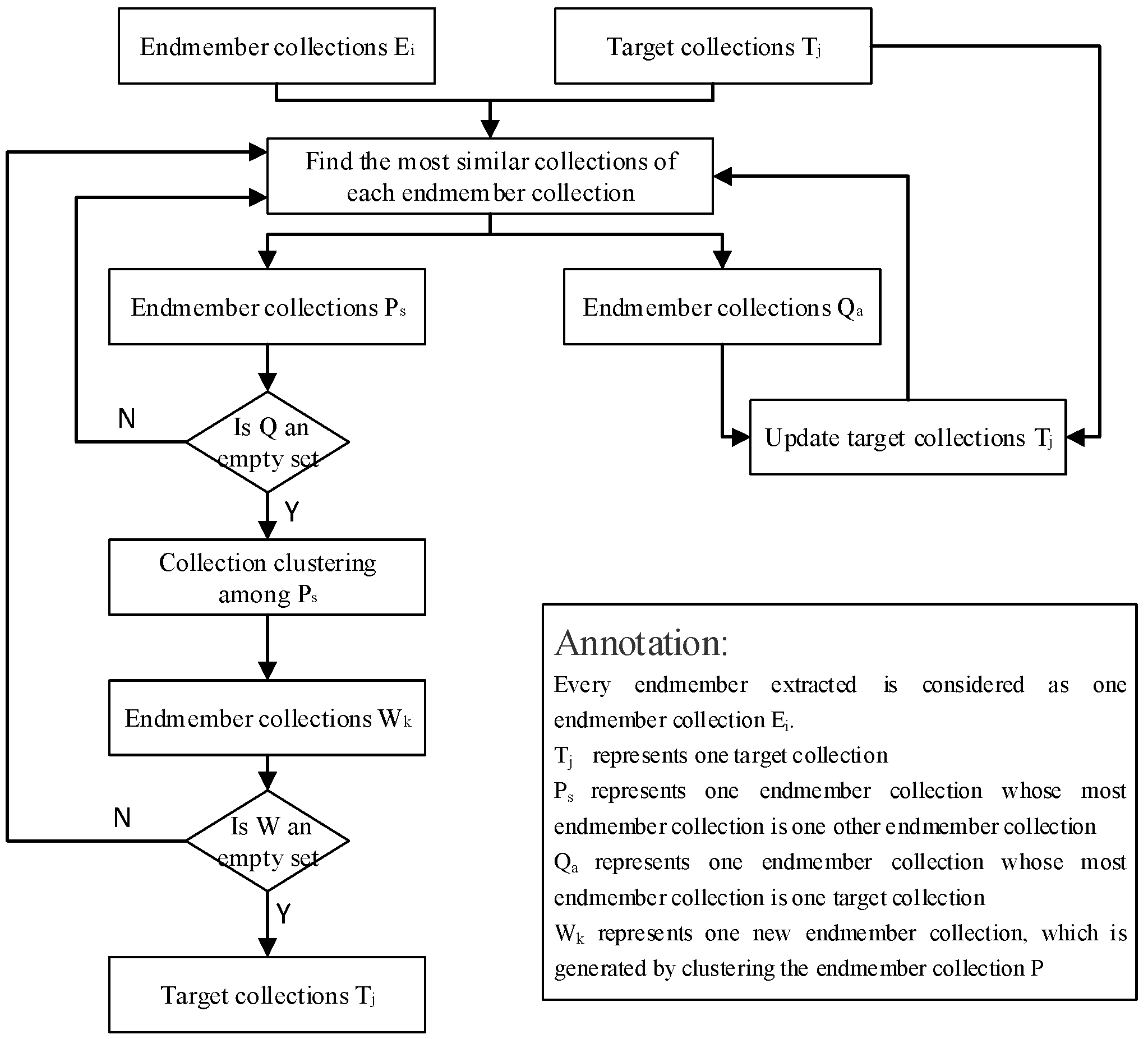
3.4. Stepwise Most Similar Collection (SMSC) Clustering

A spectral set is built after all endmembers are extracted via the above steps. The next step is to cluster endmembers in the spectral set into some collections corresponding to the various components. Automatic clustering is of great significance, as it affects accuracy evaluation and abundance estimation. The common clustering methods are not applicable to spectral sets with high spectral variability because the intraclass variation in materials may be greater than the interclass variation. In this paper, we propose a new clustering method by clustering stepwise similar endmembers to reduce the influence of spectral variability.

The main idea of this method is to use some endmembers to help their similar endmembers cluster correctly. For example, endmember i belongs to class 1 but is incorrectly assigned to class 2. In this case, endmember j, which is similar to endmember i and can be assigned correctly to class 1, can be used to help endmember i be assigned to class 1. The mathematical formula is expressed as follows:

$$\{\begin{array}{l}\mathrm{SAD}\left(\mathrm{i}, \mathrm{A}\right)>\mathrm{SAD}\left(\mathrm{i}, \mathrm{B}\right)\\ \mathrm{SAD}\left(\mathrm{j}, \mathrm{A}\right)<\mathrm{SAD}(\mathrm{j}, \mathrm{B})\\ \mathrm{SAD}\left(\mathrm{i}, \mathrm{j}\right)<\mathrm{SAD}(\mathrm{i}, \mathrm{A})\end{array},$$

(5)

where A and B represent the typical spectral signatures of class 1 and 2, respectively. These typical spectral signatures can be acquired through endmember extraction methods, field acquisition, etc. The spectral angle distance (SAD) is a metric to evaluate the similarity of two spectra, which can be calculated via Equation (6).

$$\mathrm{SAD}\left({\mathrm{x}}_{\mathrm{a}}{,\mathrm{x}}_{\mathrm{b}}\right){=\cos }^{-1}\left(\frac{{\left({\mathrm{x}}_{\mathrm{a}}\right)}^{\mathrm{T}}\cdot {\mathrm{x}}_{\mathrm{b}}}{\Vert {\mathrm{x}}_{\mathrm{a}}\Vert \cdot \Vert {\mathrm{x}}_{\mathrm{b}}\Vert }\right),$$

(6)

where $\Vert {\mathrm{x}}_{\mathrm{a}}\Vert$ and $\Vert {\mathrm{x}}_{\mathrm{b}}\Vert$ represent the norms of spectra ${\mathrm{x}}_{\mathrm{a}}$ and ${\mathrm{x}}_{\mathrm{b}}$, respectively.

The steps of SMSC clustering can be summarized as follows:

(1) Regard each endmember in the spectral set as an independent endmember collection, and take a typical spectral signature of each material as a target collection.

(2) Calculate the SAD between each spectrum in the endmember collection and all elements in the remaining collections via Equation (7), including the other endmember collections and all target collections. Collection j represents the collection which is the most similar to collection i and with the minimum SAD of collection i.

$${\mathrm{J}}_{\mathrm{i}}=\arg \underset{\mathrm{j}}{\min }{\left(\mathrm{SAD}\right(\mathrm{x}}_{\mathrm{i}}^{\mathrm{p}}{,\mathrm{x}}_{\mathrm{j}}^{\mathrm{q}}\left)\right) (\mathrm{i}=1,2,\dots {,\mathrm{N}}_1, \mathrm{j}=1,\dots ,{\mathrm{N}}_1{+\mathrm{N}}_2,\mathrm{j}\ne \mathrm{i},\mathrm{p}=1,2,\dots {\mathrm{n}}_{\mathrm{i}},\mathrm{q}=1,2,\dots ,{\mathrm{n}}_{\mathrm{j}}),$$

(7)

where ${\mathrm{x}}_{\mathrm{i}}^{\mathrm{p}}$ represents the p-th endmember in endmember collection i, ${\mathrm{x}}_{\mathrm{j}}^{\mathrm{q}}$ represents the q-th element in collection j, N₁ and N₂ represent the number of endmember collections and target collections, respectively, and n_i and n_j represent the number of spectra in collection i and j.

(3) Merge endmember collections, whose most similar collections are target collections, into the corresponding target collection, and update target collections.

(4) Repeat steps (2)–(3) until no endmember collections can be merged into target collections.

(5) Merge each remaining endmember collection with its corresponding most similar endmember collection, and update endmember collections. Then, repeat steps (2)–(4) until all endmember collections are merged into the target collections.

The specific process of the SMSC clustering method is shown in Figure 3.

The proposed SMSC clustering method gradually clusters extracted endmembers into target collections according to steps (3) and (4) instead of directly clustering all endmembers into some categories. At each step of clustering, the number of endmembers in the target collection gradually increases with the enhancement of the spectral variability, which indirectly helps the remaining endmembers cluster. According to stepwise clustering, the spectral variability of extracted endmembers will be dispersed in each clustering.

4. Experiments and Analysis

This section describes the experiments performed on both a synthetic dataset and real datasets. These experiments can demonstrate a comprehensive comparison between the proposed method and other typical methods.

In this paper, we adopted the mean spectral angle distance (MSAD) to valuate extracted endmembers and root-mean-square error (RMSE) to assess the reconstructed image and estimated abundance.

MSAD can be calculated via Equation (8),

$$\mathrm{MSAD}=\frac{1}{\mathrm{M}}{\displaystyle \sum _{\mathrm{i}=1}^{\mathrm{M}}{\cos }^{-1}\left(\frac{{\mathrm{x}}_{\mathrm{i}}{}^{\mathrm{T}}\cdot {\hat{\mathrm{x}}}_{\mathrm{i}}}{\Vert {\mathrm{x}}_{\mathrm{i}}\Vert \cdot \Vert {\hat{\mathrm{x}}}_{\mathrm{i}}\Vert }\right)},$$

(8)

where M is the number of extracted endmembers, ${\hat{\mathrm{x}}}_{\mathrm{i}}$ denotes the extracted endmember, and ${\mathrm{x}}_{\mathrm{i}}$ is the corresponding ground truth.

RMSE was used to evaluate the performance of various methods. It is given by Equation (9),

$$\mathrm{RMSE}\left(\mathrm{z},\hat{\mathrm{z}}\right)={\left(\frac{1}{\mathrm{N}}{\Vert \mathrm{z}- \hat{\mathrm{z}}\Vert }_2^2\right)}^{\frac{1}{2}},$$

(9)

where N is the number of elements in z, z is the truth including the true abundance and original hyperspectral image, and $\widehat{z}$ represents the corresponding estimated result. A smaller RMSE corresponds to a better performance. In this paper, RMSE_R represents the RMSE between reconstructed image and original image, whereas RMSE_A represents the RMSE between true abundance and estimated abundance.

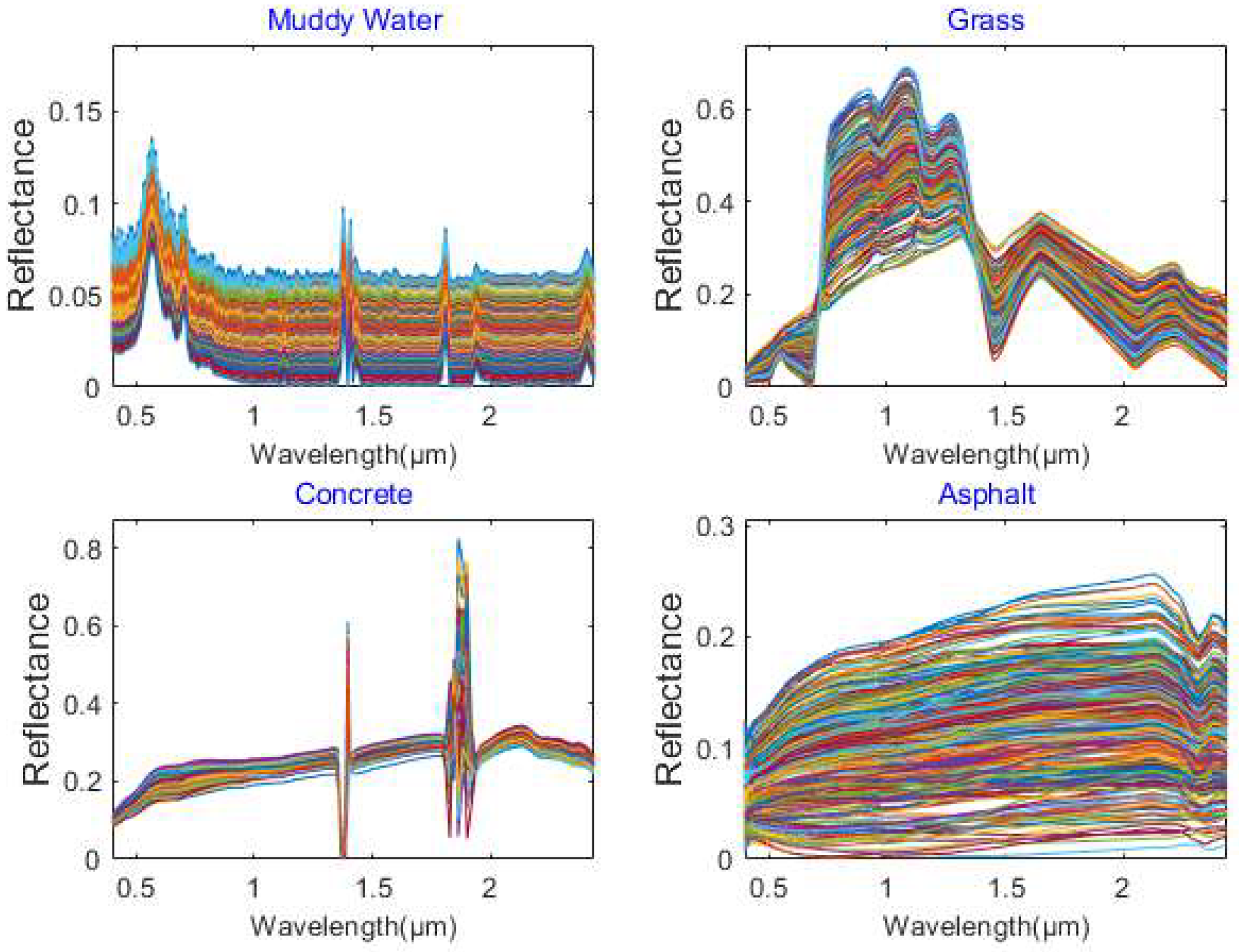
4.1. Synthetic Image Dataset

The endmembers of the synthetic hyperspectral image were selected from the DIRSIG spectral library [38] with high spectral variability. Figure 4 displays the spectral library of the four materials used in this paper. The simulated data contained four features including muddy water, grass, asphalt, and concrete. 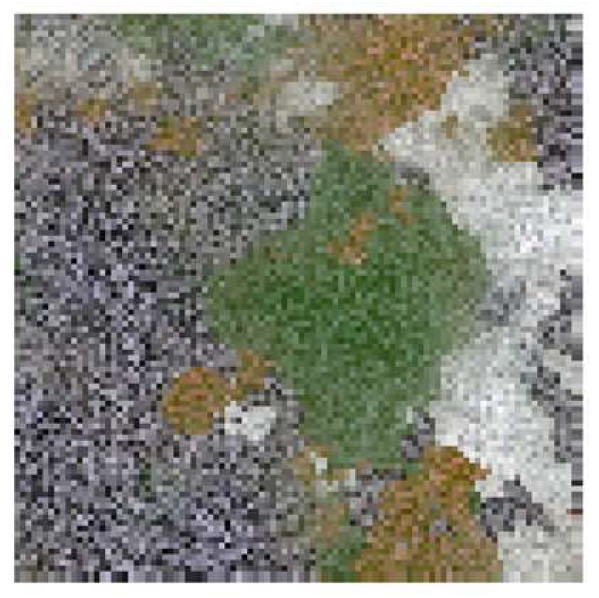The corresponding spatially correlated abundances were generated from a Gaussian random field [39]. Moreover, there was only one pure pixel of each material according to the above abundance generation method. To simulate the spectral variability of the synthetic image, we modified the abundance of a material greater than 0.95 to 1 and the abundance of other materials to 0. The spectrum of each pixel in the synthetic hyperspectral data is the sum of the spectral signature of various materials weighted by their corresponding abundances. The synthetic hyperspectral image generated by the above steps complies with the abundance non-negativity constraint (ANC) and abundance sum-to-one constraint (ASC). The simulated hyperspectral image is exhibited in Figure 5.

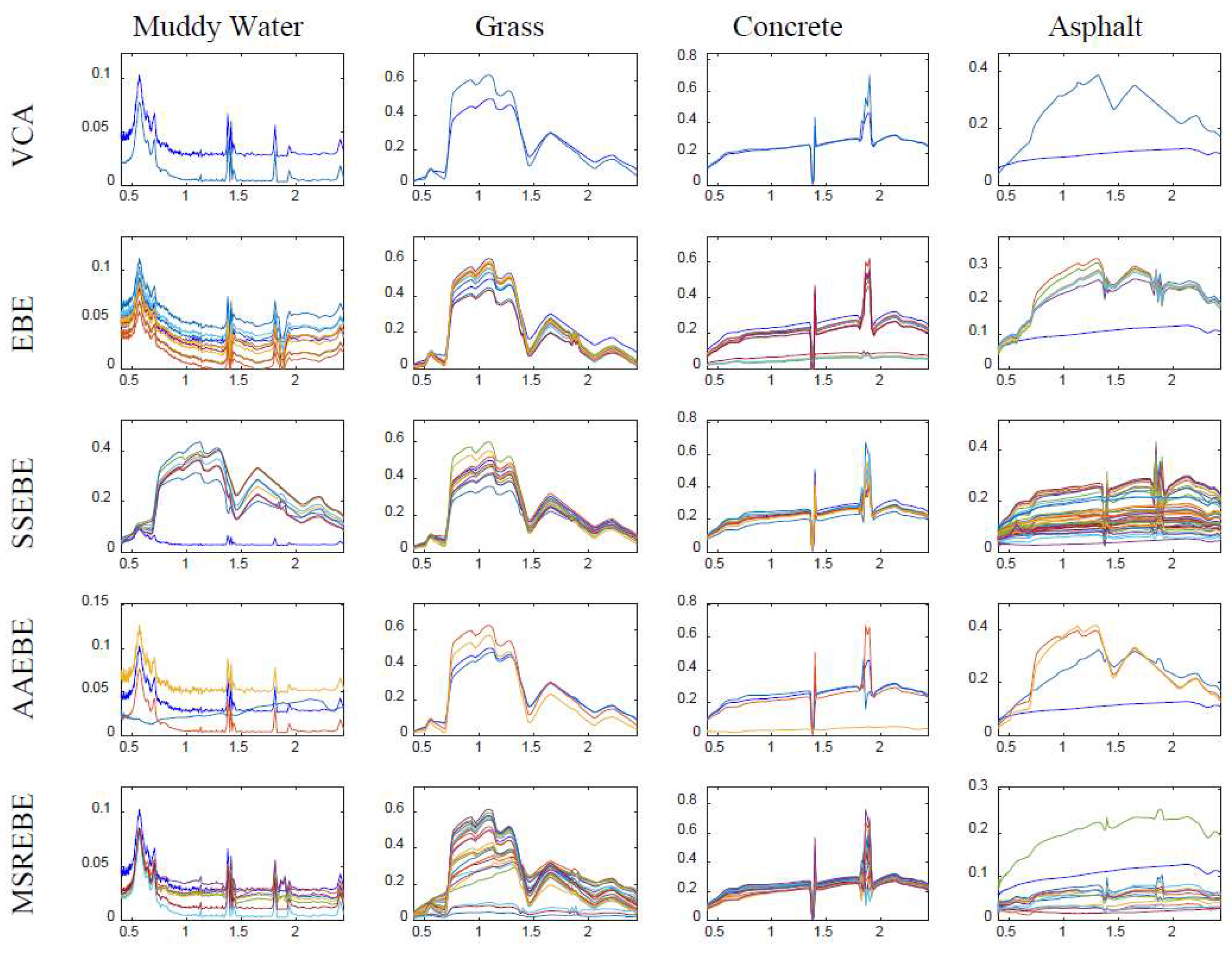
There are some points to be noted in this experiment: (1) in the EBE method, the number of subsets generated from the original image was set to 10; (2) in AAEBE and SSEBE, the number of projections used to extract candidate endmembers was set to 10,000, and the threshold was set to 0; (3) the number of endmembers in each material was set to 3 in AAEBE. 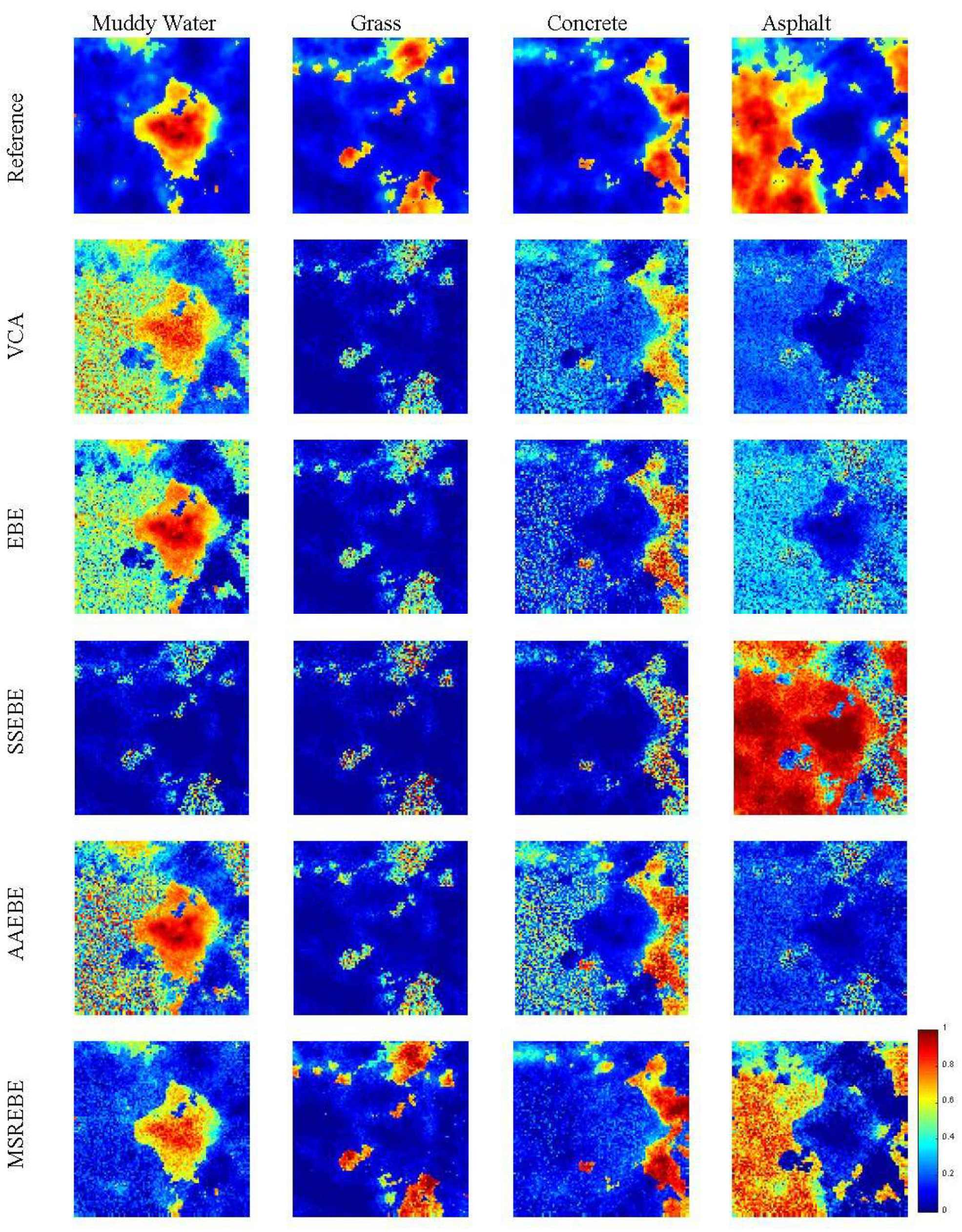The extraction results of the five methods are presented in Figure 6. To comprehensively compare the extraction methods, we added abundance estimation experiments. Fully constrained least squares (FCLS) was chosen as the method to estimate abundance in this paper, which can avoid the influence of parameter selection. The estimation results are shown in Figure 7.

Table 1. Experimental results of synthetic image dataset.

Methods	MSAD	RMSER	RMSEA
VCA	0.221	0.178	0.208
EBE	0.167	0.124	0.168
SSEBE	0.247	0.072	0.214
AAEBE	0.277	0.035	0.208
MSREBE	0.155	0.067	0.037

presents the results of comparison between MSREBE and the other methods as a function of three metrics, and the best performance is bolded.

Figure 4 demonstrates that all four materials contained high spectral variability, especially asphalt, thus hindering the extraction of endmember bundle associated with asphalt. Comparing the extracted results in Figure 6 with the ground truth in Figure 4, the extracted endmembers of asphalt by VCA, EBE, and AAEBE were far from the associated ground truth, while MSREBE and SSEBE extracted partial endmembers of asphalt. It can also be seen from Figure 6 that the extraction result of MSREBE was better than that of SSEBE. In addition, the abundance maps related to MSREBE better agreed with the true abundance maps shown in Figure 7. Table 1 indicates that MSREBE was second only to AAEBE in terms of the RMSE of reconstruction error. Nevertheless, it was superior to other methods in terms of the RMSE of abundance error and MSAD. Considering the above, the proposed method performed better than other methods using the synthetic dataset.

4.2. Wetland Dataset

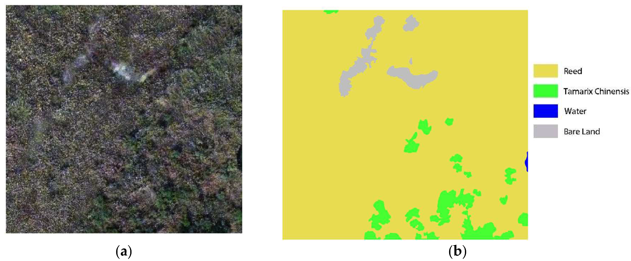
The original hyperspectral image was taken on 25 October 2020 in Dongying by an unmanned aerial vehicle hyperspectral camera. The wetland dataset with a size of 263 × 271, shown in Figure 8a, was a subset of the original hyperspectral image with 126 bands, covering the wavelength range of 0.450–0.946 μm. There were main four materials including reed, tamarix chinensis, bare land, and water in the wetland dataset. In this paper, the corresponding ground truth of the study area was drawn on the basis of a multispectral image with higher spatial resolution in the same area (as shown in Figure 8b).

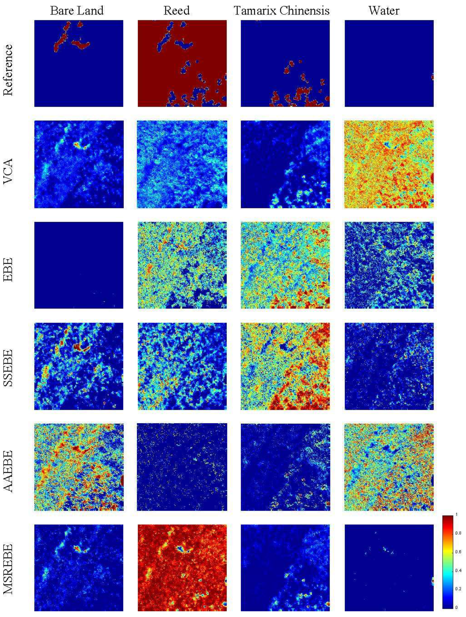
In Figure 9, the extraction results of VCA, EBE, SSEBE, AAEBE, and the proposed method are shown from top to bottom. As in the simulated hyperspectral data experiment, the abundance estimation was performed by FCLS with endmembers extracted using the five methods, and the abundance maps are presented in Figure 10.

Table 2. Experimental results of wetland dataset.

Methods	MSAD	RMSER	RMSEA
VCA	0.279	0.067	0.382
EBE	0.224	0.178	0.321
SSEBE	0.312	0.039	0.349
AAEBE	0.291	1.107	0.479
MSREBE	0.089	0.019	0.073

indicates the comparison results between MSREBE and the other methods.

Figure 8 demonstrates that the area of water was obviously smaller than other features, which means that it was difficult to extract the endmember bundle corresponding to water. From Figure 9, we can find that all methods could adequately extract the endmembers of various materials except for water. By comparing the endmembers extracted using various methods, we can find that the water endmember bundle extracted by the proposed method was better than that extracted by other methods. Figure 10 presents the abundance maps of different methods; the first row is the reference abundance, followed by the results of VCA, EBE, SSEBE, AAEBE, and MSREBE. By comparing the abundance maps associated with various methods with the reference maps, it can be found that the results of MSREBE were closer to the reference abundance maps than the other methods, especially for reeds and water. Table 2 demonstrates the comparison between MSREBE and other methods as a function of various metrics, and the best results are marked in bold. From Table 2, we can see that the MSREBE achieved the best results in terms of all evaluation indicators, again indicating its superiority to other methods in hyperspectral unmixing with high spectral variability. Comparing Table 1 with Table 2, we can find that the proposed method is more suitable for wetland data. The first reason behind this phenomenon is that the spectral variability of the wetland dataset was so large that it was difficult to adequately express with relatively few endmembers, for example, VCA and EBE. The second reason is that the spectral characteristics of reed and tamarix chinensis were relatively similar, and traditional clustering methods struggled to correctly cluster the endmembers of similar materials.

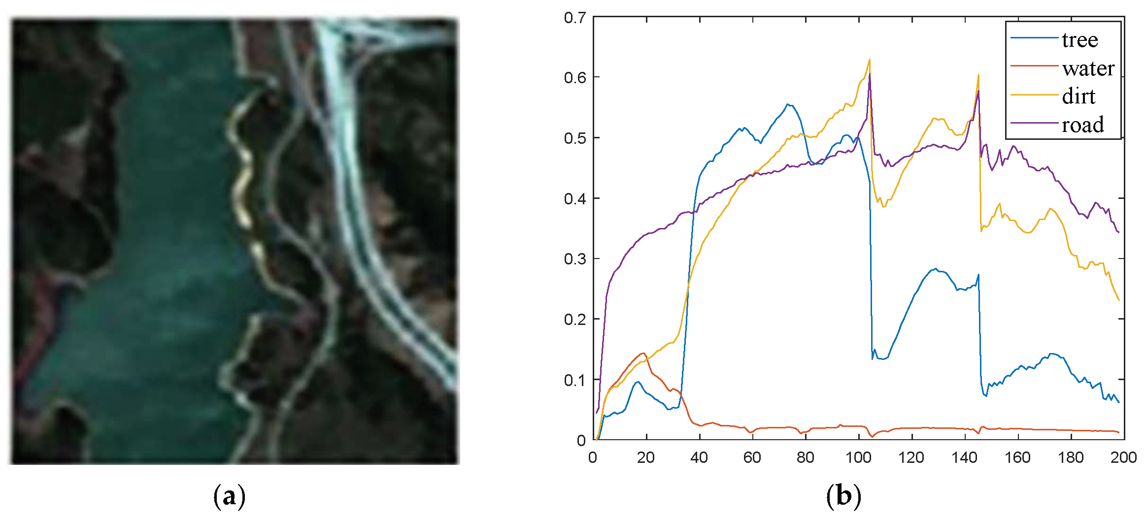
4.3. Jasper Ridge Dataset

Jasper Ridge is a popular hyperspectral dataset used in unmixing. The original image has a size of 512 × 614, with 224 channels ranging from 380 nm to 2500 nm. The spectral resolution is up to 9.46 nm [40]. In this paper, a sub-image of 100 × 100 pixels was used to conduct relative experiments after removing some channels susceptible to dense water vapor and atmosphere. There were four main features in the experimental area. Figure 11 exhibits the true color image of the experimental area and the ground truth.

Table 3. Experimental results of Jasper Ridge dataset.

Methods	MSAD	RMSER	RMSEA
VCA	0.163	0.159	0.102
EBE	0.356	0.252	0.188
SSEBE	0.121	0.109	0.043
AAEBE	0.225	0.127	0.082
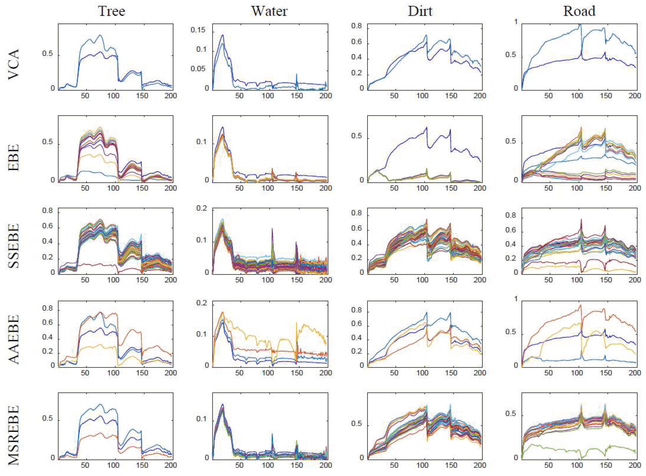
MSREBE	0.099	0.140	0.036

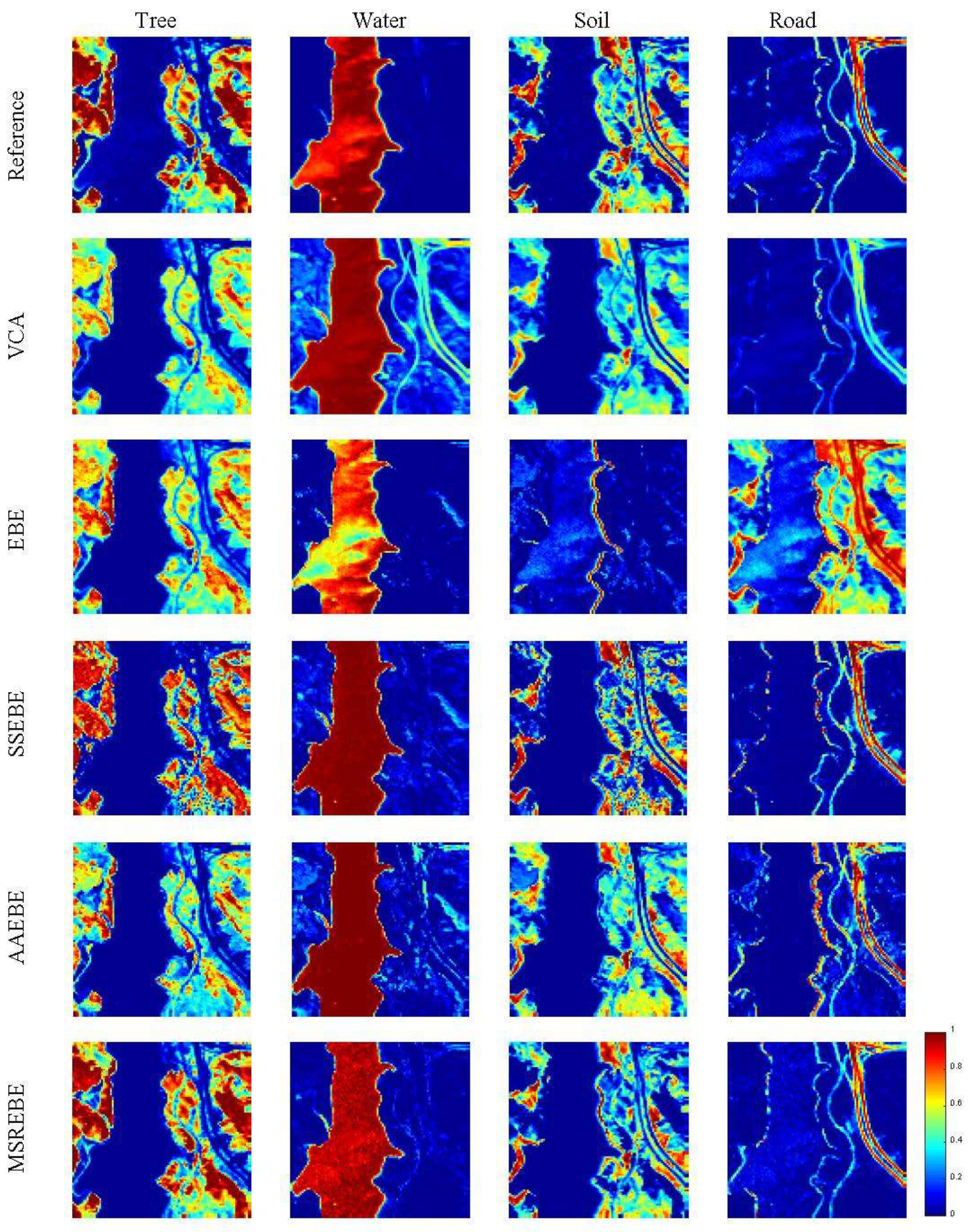
presents a comparison based on three indicators calculated using the endmembers obtained by VCA, EBE, SSEBE, AAEBE, and MSREBE. The best performance is bolded. Figure 12 and Figure 13 show the extracted endmembers and the abundance maps corresponding to various methods.

The endmembers extracted by various methods indicate that the spectral variability was relatively lower than that of the other two datasets, which resulted in the advantages of the proposed method not being fully shown. In addition, in Figure 11a, we can see that the distributions of ground objects in this dataset were more complex than in other datasets. Therefore, more boundary pixels were deleted by MSREBE, which caused the spectral variability within endmembers extracted by MSREBE to be lower than within those extracted by SSEBE (as shown in Figure 12), as well as led to a relatively high RMSE between the original image and reconstructed image. However, the performances of MSREBE in terms of RMSE_A and MSAD show that MSREBE extracted effective endmembers of various materials which were more suitable for unmixing. The corresponding abundance maps of various methods are compared in Figure 13. It is not difficult to find that the abundance maps corresponding to MSREBE were more similar to the reference, again proving the effectiveness of the proposed method.

4.4. Washington DC Mall Dataset

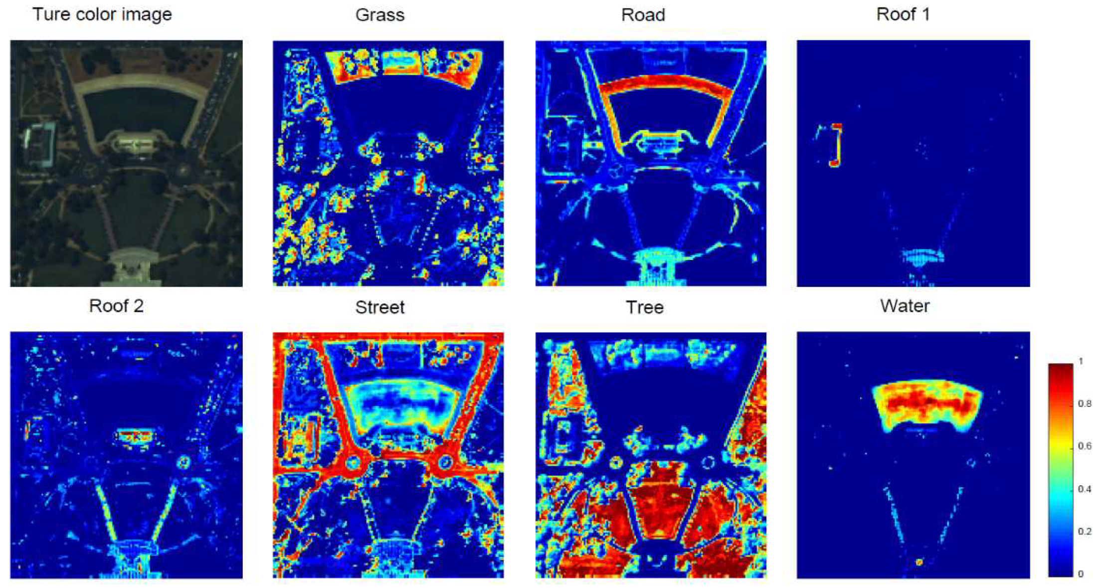
In this section, we performed relative experiments using Washington DC Mall dataset, which was collected by the Spectral Information Technology Application Center of Virginia with the Hyperspectral Digital Imagery Collection Experiment (HYDICE) sensor. Each pixel was recorded in 210 channels ranging from 400 nm to 2400 nm. After stripping out some bands affected by the atmosphere or with high noise, 191 bands remained in the dataset. In this experiment, a subset of 151 × 141 was extracted from the original image. The subscene mainly included seven types of ground objects, namely, grass, road, water, tree, street, roof 1, and roof 2. Figure 14 shows the true color image of study area and some pure pixels selected manually corresponding to the seven features. The spectral averages of the pure pixels corresponding to various endmembers were calculated as the reference endmember signatures. Due to the lack of true abundance of this dataset, only MSAD and RMSE were used to evaluate the proposed method and other typical methods. The result is shown in

Table 4. Experimental results of Washington DC Mall dataset.

Methods	MSAD	RMSER
VCA	0.244	0.308
EBE	0.152	0.016
SSEBE	0.225	0.095
AAEBE	0.143	0.026
MSREBE	0.081	0.021

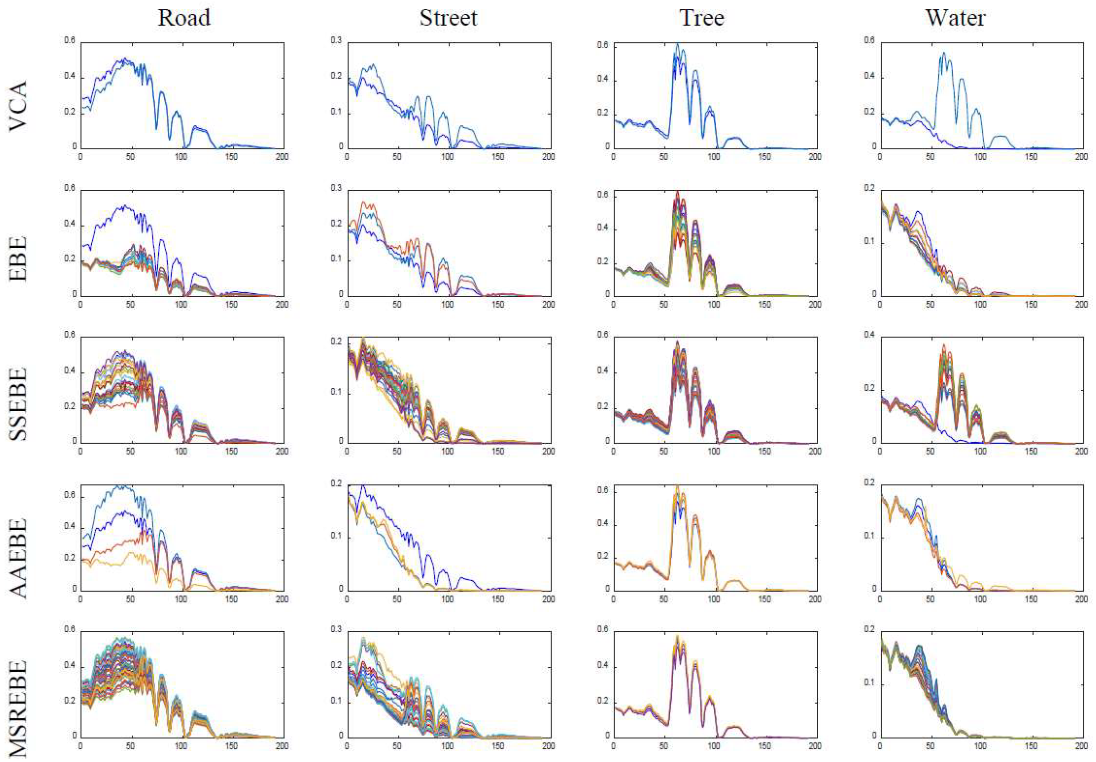
, where the best performance is bolded. Figure 15 shows the four endmember extraction results corresponding to various methods, and Figure 16 shows the abundance result of Washington DC Mall estimated by the proposed method.

The Washington DC Mall dataset was different from the previous three datasets; it had more types of features and a more complex feature distribution. According to Table 4, we can find that MSREBE had the best performance in terms of MSAD among all methods and was second only to EBE in the RMSE of the reconstruction error. From Figure 15, it is not difficult to find that MSREBE had a better extraction effect than other methods. Although there were no real abundance maps, we can find that the estimated abundance maps could approximately represent the ground object distribution of the real image. According to the above experimental results, we can conclude that the proposed method can not only be used in scenes with fewer features, but also in complex scenes with several ground objects.

4.5. Discussion

From the above experiments with a synthetic dataset and real datasets, we can observe that, firstly, the proposed method had a lower mean SAD than the comparison methods, and the abundance estimation experiments showed that the abundance maps corresponding to MSREBE were more consistent with the references, again reflecting the superiority of MSREBE in hyperspectral unmixing. Secondly, the proposed method is applicable to a variety of scenarios, not only for a scene with large differences in ground feature distribution, such as the wetland dataset, but also to a scene with complex ground feature distribution or several features, such as the Jasper Ridge and Washington DC Mall datasets. However, there are still some unresolved issues. Relevant parameters are difficult to determine. The sampling scales and threshold play a significant role in MSREBE. However, these parameters were determined through multiple tests in this paper. In our future work, we will try different methods to determine the best sampling scales for various datasets. So far, we have found that the sampling scales should be related to the size of the hyperspectral image, the degree of spectral variability, and the complexity of the ground feature distribution. In further research, we will try to adaptively determine the sampling scales according to the characteristics of the image. Through many experiments, we found that it is appropriate to select candidate endmembers using one-third of the sampling scale number as the threshold. However, the threshold may be changed as a function of the rules governing the sampling scales.

5. Conclusions

In this paper, a novel multiscale resampling endmember bundle extraction (MSREBE) algorithm was proposed for hyperspectral endmember bundle extraction. To address spectral variability within hyperspectral unmixing, some strategies were employed. We performed endmember extraction in sections of sub-images with much lower spectral variability. Then, the pixels selected as candidate endmembers at multiple sampling scales were taken as endmembers. A novel stepwise most similar collection (SMSC) clustering method was proposed. The extracted endmembers were clustered stepwise on the basis of minimum SAD. In each clustering, each endmember collection was only merged with the corresponding most similar collection, which could weaken the influence of spectral variability within extracted endmembers. The experiments performed in this paper proved that the proposed method has strong practicability and can be applied to a variety of datasets, obtaining better results than other algorithms.