
Ecological Safety Assessment and Analysis of Regional Spatiotemporal Differences Based on Earth Observation Satellite Data in Support of SDGs: The Case of the Huaihe River Basin

 ,
, 
Abstract
:
1. Introduction
2. Materials and Methods
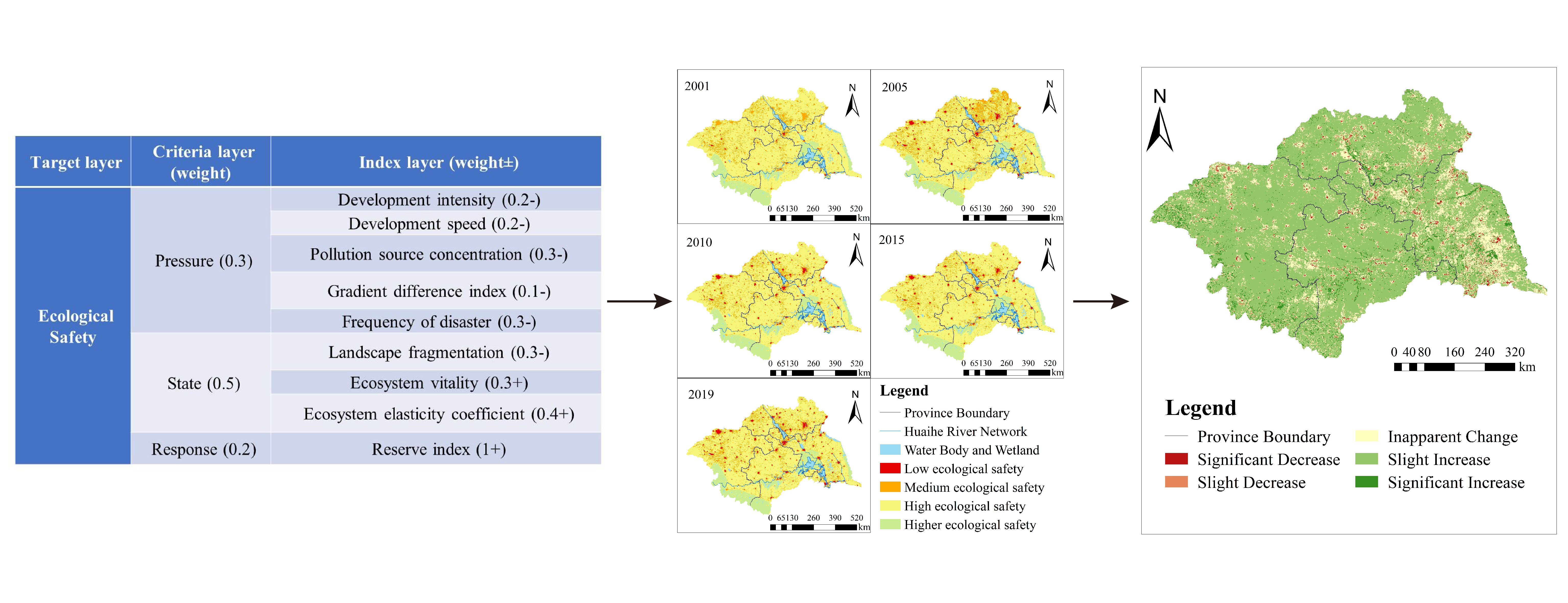
2.1. Study Area
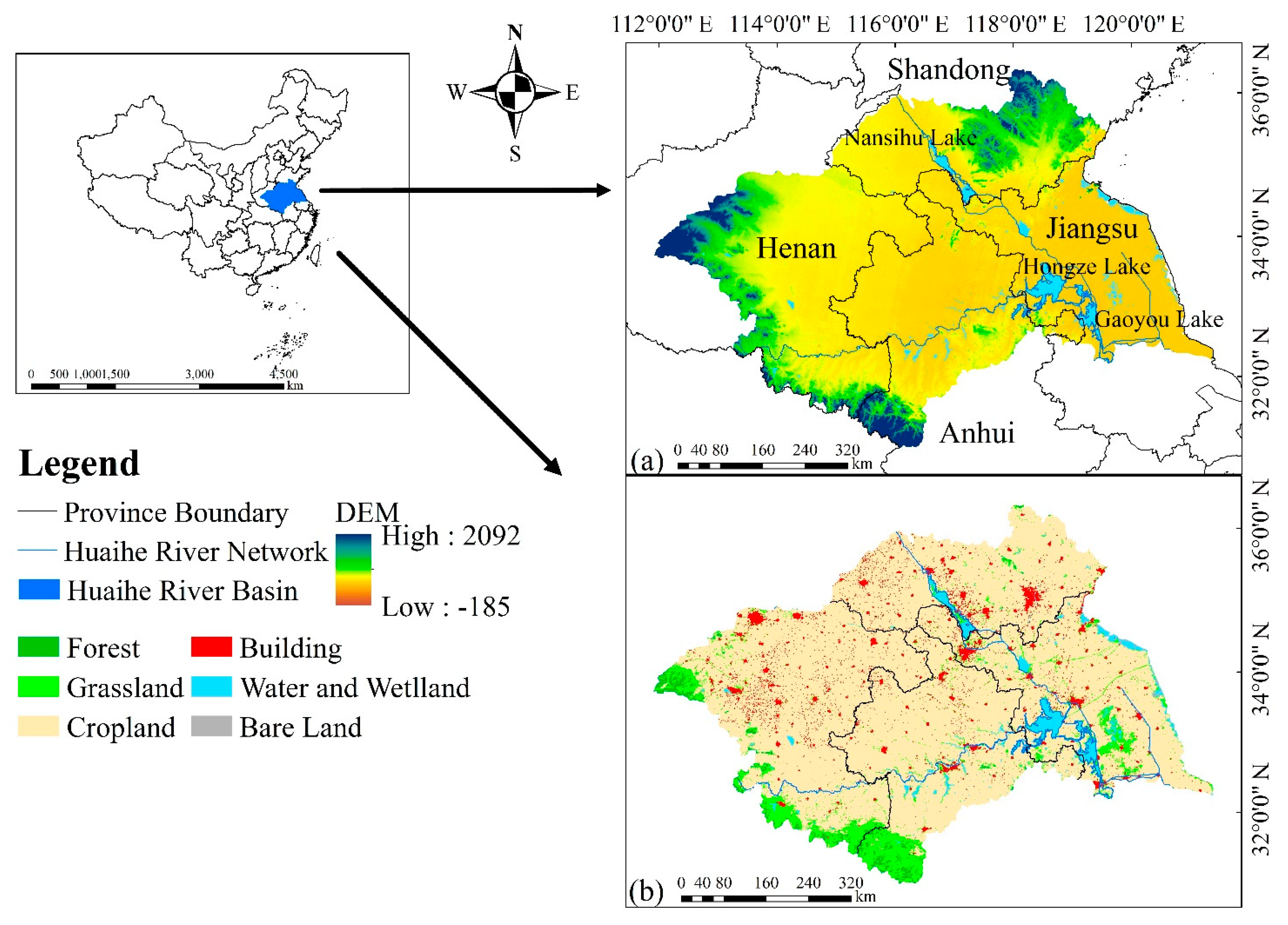
2.2. Workflow
2.3. Establishment of the ES Assessment System
2.3.1. Indicator Calculation
2.3.2. Determination of Weights
2.4. Data Sources and Processing
2.4.1. Data Sources
2.4.2. Data Normalization
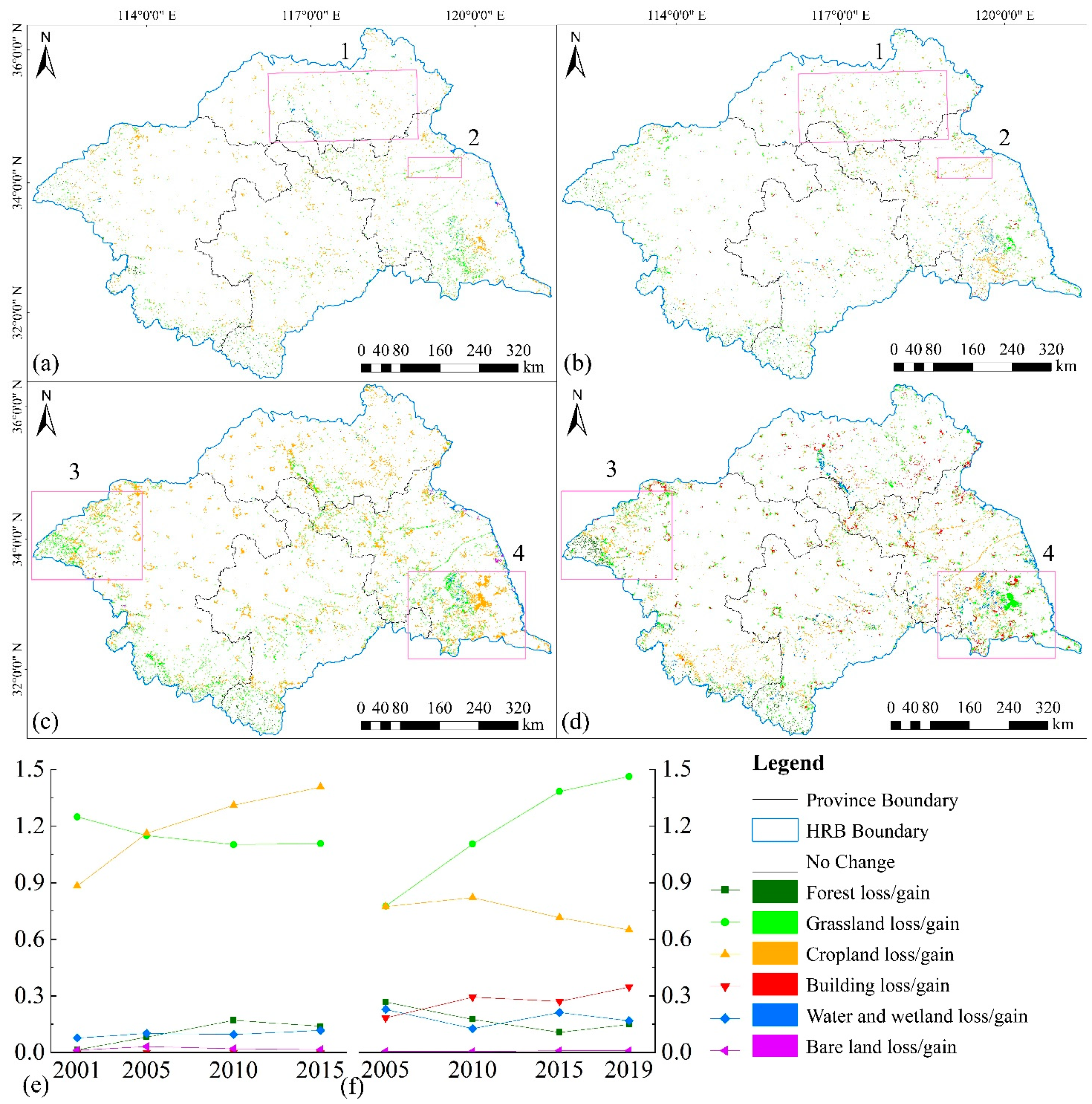
2.4.3. Land Change Analysis
2.4.4. Trend Analysis
2.4.5. Correlation Analysis
3. ES Assessment Results for the HRB
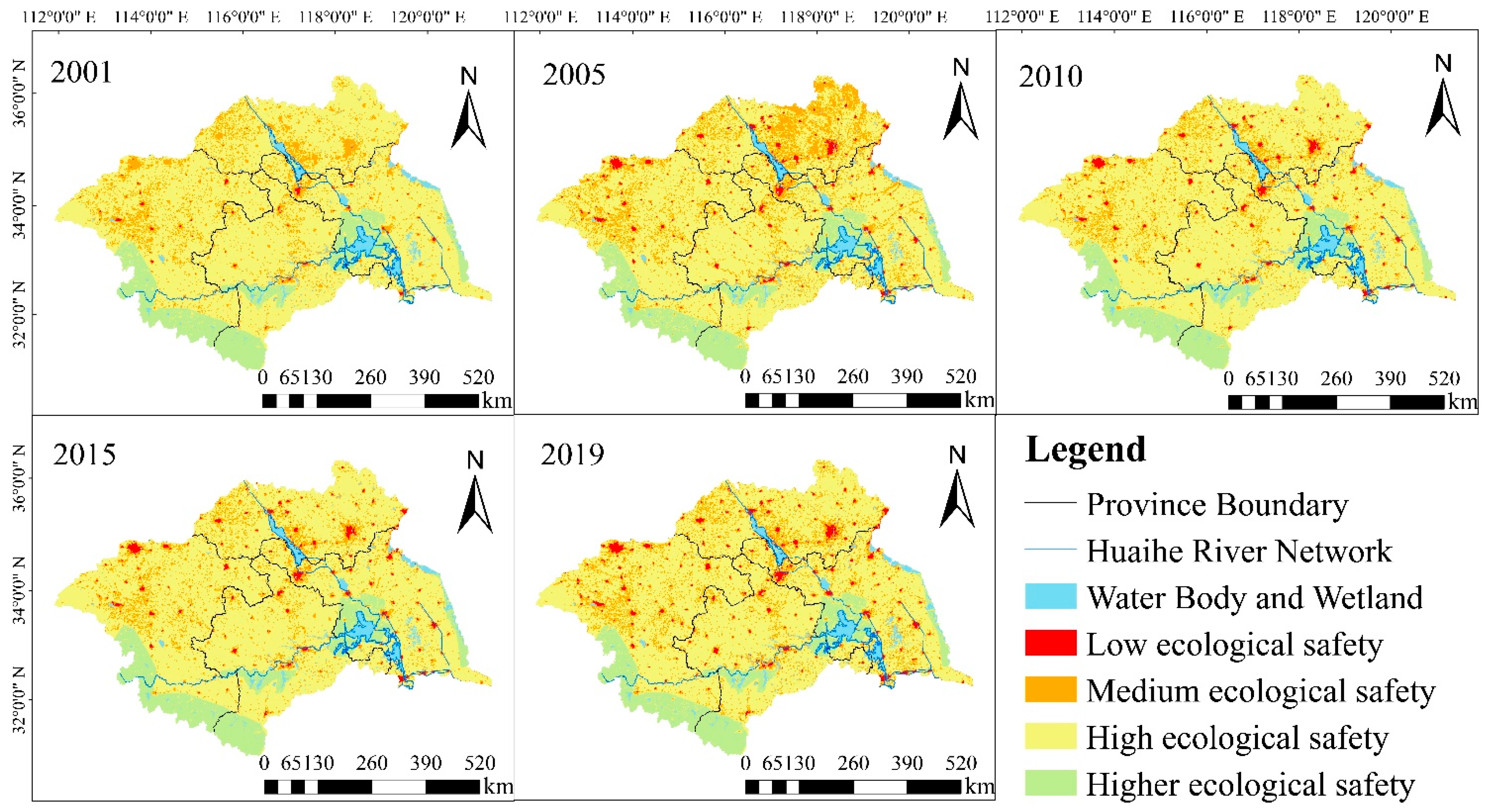
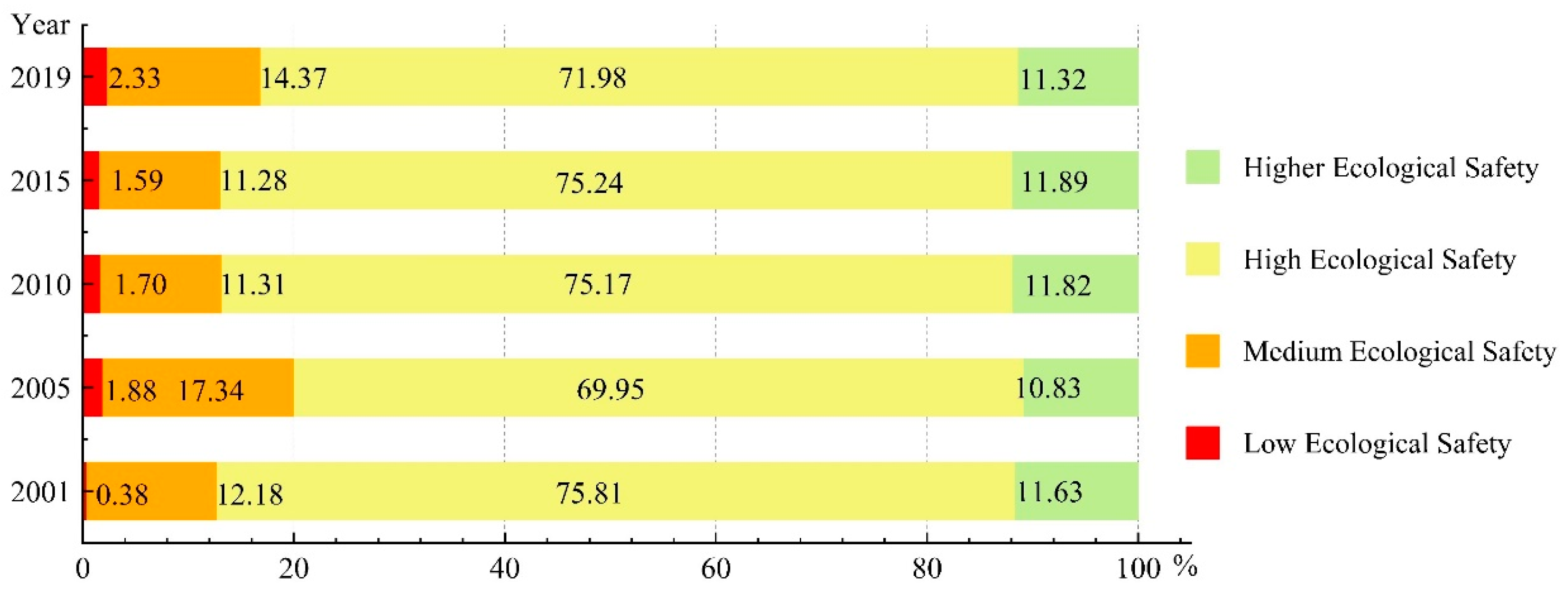
3.1. Overall Spatiotemporal Variations in ES of the HRB
3.2. Variations of ES in the Four Provinces
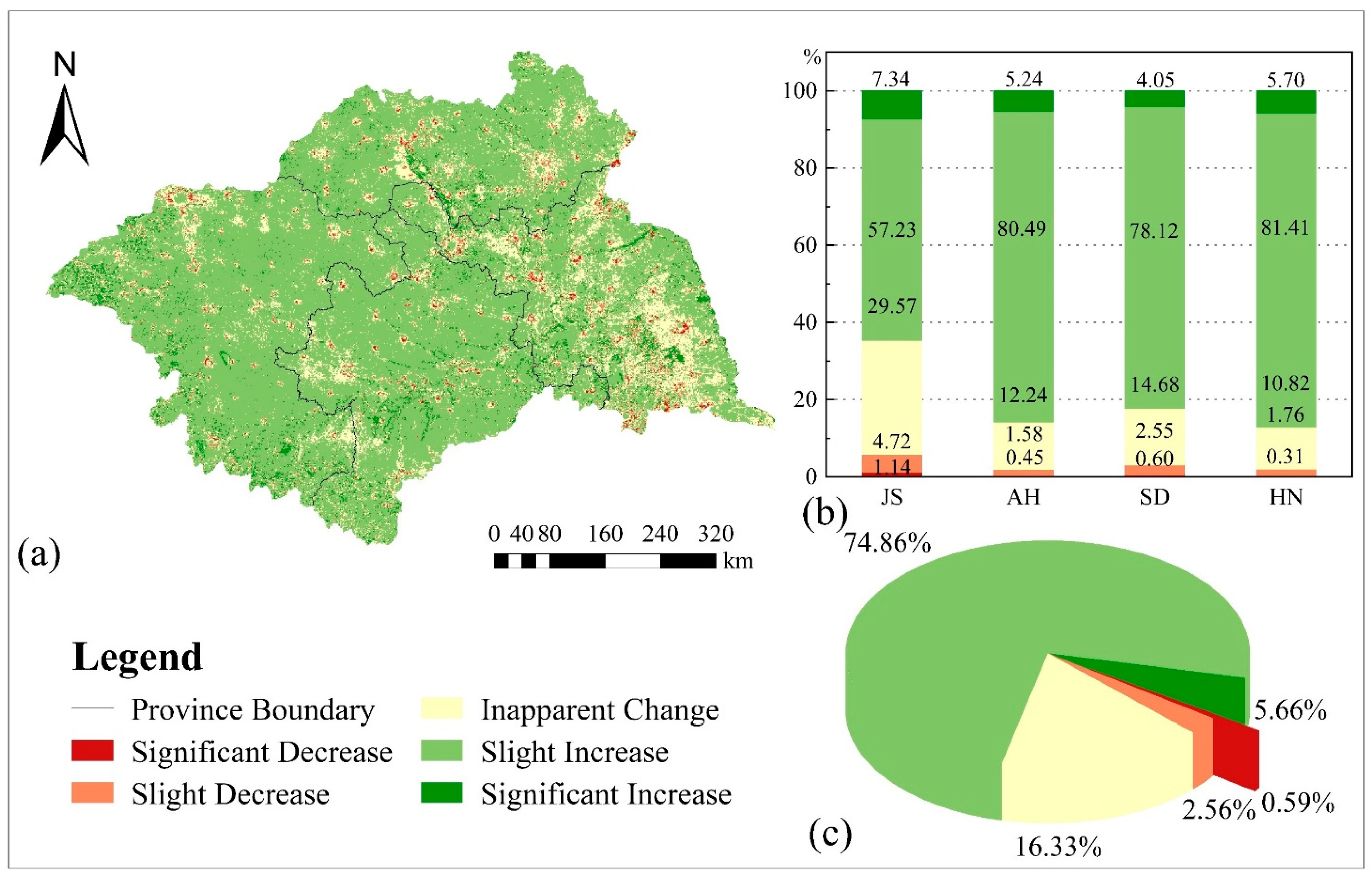
3.3. Trends in ES Value of the HRB
4. Discussion
4.1. The Indicator System to Evaluate Sustainable Development of Basins
4.2. Analysis of the Factors Influencing Sustainable Development in the HRB
4.3. Moving toward Achieving SDGs of the HRB
5. Conclusions
Author Contributions
Funding
Institutional Review Board Statement
Informed Consent Statement
Acknowledgments
Conflicts of Interest
References
- Nations, U. Transforming Our World: The 2030 Agenda for Sustainable Development. 2015. Available online: https://sustainabledevelopment.un.org/post2015/transformingourworld/publication (accessed on 10 October 2020).
- Rosati, F.; Faria, L.G. Addressing the SDGs in sustainability reports: The relationship with institutional factors. J. Clean. Prod. 2019, 215, 1312–1326. [Google Scholar] [CrossRef]
- Allen, C.; Metternicht, G.; Wiedmann, T. Initial progress in implementing the Sustainable Development Goals (SDGs): A review of evidence from countries. Sustain. Sci. 2018, 13, 1453–1467. [Google Scholar] [CrossRef]
- Peng, K.; Jiang, W.; Ling, Z.; Hou, P.; Deng, Y. Evaluating the potential impacts of land use changes on ecosystem service value under multiple scenarios in support of SDG reporting: A case study of the Wuhan urban agglomeration. J. Clean. Prod. 2021, 127321. [Google Scholar] [CrossRef]
- Cheng, G.; Li, X. Integrated research methods in watershed science. Sci. China Earth Sci. 2015, 58, 1159. [Google Scholar] [CrossRef]
- Postel, S.L.; Thompson, B.H., Jr. Watershed protection: Capturing the benefits of nature’s water supply services. Nat. Resour. Forum 2005, 29, 98–108. [Google Scholar] [CrossRef]
- Wang, H.; Meijerink, S.; van der Krabben, E. Institutional Design and Performance of Markets for Watershed Ecosystem Services: A Systematic Literature Review. Sustainability 2020, 12, 6382. [Google Scholar] [CrossRef]
- Reith, J.; Ghazaryan, G.; Muthoni, F.; Dubovyk, O. Assessment of Land Degradation in Semiarid Tanzania—Using Multiscale Remote Sensing Datasets to Support Sustainable Development Goal 15.3. Remote Sens. 2021, 13, 1754. [Google Scholar] [CrossRef]
- Cherrington, E.A.; Griffin, R.E.; Anderson, E.R.; Sandoval, B.E.H.; Flores-Anderson, A.I.; Muench, R.E.; Markert, K.N.; Adams, E.C.; Limaye, A.S.; Irwin, D.E. Use of public Earth observation data for tracking progress in sustainable management of coastal forest ecosystems in Belize, Central America. Remote Sens. Environ. 2020, 245, 111798. [Google Scholar] [CrossRef]
- Bian, J.; Li, A.; Nan, X.; Lei, G.; Zhang, Z. Dataset of the mountain green cover index (SDG15.4.2) over the economic corridors of the Belt and Road Initiative for 2010–2019. Big Earth Data 2021, 1–13. [Google Scholar] [CrossRef]
- Wang, H.; Long, H.; Li, X.; Yu, F. Evaluation of changes in ecological security in China’s Qinghai Lake Basin from 2000 to 2013 and the relationship to land use and climate change. Environ. Earth Sci. 2014, 72, 341–354. [Google Scholar] [CrossRef]
- Wen, M.; Zhang, T.; Li, L.; Chen, L.; Hu, S.; Wang, J.; Liu, W.; Zhang, Y.; Yuan, L. Assessment of Land Ecological Security and Analysis of Influencing Factors in Chaohu Lake Basin, China from 1998–2018. Sustainability 2021, 13, 358. [Google Scholar] [CrossRef]
- Liu, D.; Chang, Q. Ecological security research progress in China. Acta Ecol. Sin. 2015, 35, 111–121. [Google Scholar] [CrossRef]
- Linster, M.; Fletcher, J. Using the Pressure-State-Response Model to Develop Indicators of Sustainability: OECD Framework for Environmental Indicators. Organ. Econ. Co Oper. Dev. Paris 2001, 11. [Google Scholar]
- UN. United Nations Indicators of Sustainable Development; Framework and Methodologies; UNCSD: Rio de Janeiro, Brazil, 1996. [Google Scholar]
- OECD. Environment Indicators—Development, Measurement and Use; Organisation of Economic Co-operation and Development; OECD: Paris, France, 2003. [Google Scholar]
- Kelble, C.R.; Loomis, D.K.; Lovelace, S.; Nuttle, W.K.; Ortner, P.B.; Fletcher, P.; Cook, G.S.; Lorenz, J.J.; Boyer, J.N. The EBM-DPSER conceptual model: Integrating ecosystem services into the DPSIR framework. PLoS ONE 2013, 8, e70766. [Google Scholar] [CrossRef] [Green Version]
- Tang, Y.; Zhao, X.; Jiao, J. Ecological security assessment of Chaohu Lake Basin of China in the context of River Chief System reform. Environ. Sci. Pollut. Res. 2020, 27, 2773–2785. [Google Scholar] [CrossRef] [PubMed]
- Hua, Y.; Yan, M.; Limin, D. Land ecological security assessment for Bai autonomous prefecture of Dali based using PSR model--with data in 2009 as case. Energy Procedia 2011, 5, 2172–2177. [Google Scholar] [CrossRef] [Green Version]
- Shao, C.; Guan, Y.; Chu, C.; Shi, R.; Ju, M.; Shi, J. Trends analysis of ecological environment security based on DPSIR model in the coastal zone: A survey study in Tianjin, China. Int. J. Environ. Res. 2014, 8, 765–778. [Google Scholar] [CrossRef] [Green Version]
- Bai, X.; Tang, J. Ecological security assessment of Tianjin by PSR model. Procedia Environ. Sci. 2010, 2, 881–887. [Google Scholar] [CrossRef] [Green Version]
- Ma, L.; Bo, J.; Li, X.; Fang, F.; Cheng, W. Identifying key landscape pattern indices influencing the ecological security of inland river basin: The middle and lower reaches of Shule River Basin as an example. Sci. Total Environ. 2019, 674, 424–438. [Google Scholar] [CrossRef]
- Du, P.; Xia, J.; Du, Q.; Luo, Y.; Tan, K. Evaluation of the spatio-temporal pattern of urban ecological security using remote sensing and GIS. Int. J. Remote Sens. 2013, 34, 848–863. [Google Scholar] [CrossRef]
- Zhao, Y.-Z.; Zou, X.-Y.; Cheng, H.; Jia, H.-K.; Wu, Y.-Q.; Wang, G.-Y.; Zhang, C.-L.; Gao, S.-Y. Assessing the ecological security of the Tibetan plateau: Methodology and a case study for Lhaze County. J. Environ. Manag. 2006, 80, 120–131. [Google Scholar] [CrossRef] [PubMed]
- Wei, W.; Xie, B.B. Evaluation of the ecological security in Shiyang River Basin based on Grid GIS and PSR model. Adv. Mater. Res. 2014, 80, 1042–1046. [Google Scholar] [CrossRef]
- Wu, X.; Liu, S.; Sun, Y.; An, Y.; Dong, S.; Liu, G. Ecological security evaluation based on entropy matter-element model: A case study of Kunming city, southwest China. Ecol. Indic. 2019, 102, 469–478. [Google Scholar] [CrossRef]
- Saaty, T.L. How to make a decision: The analytic hierarchy process. Eur. J. Oper. Res. 1990, 48, 9–26. [Google Scholar] [CrossRef]
- Saaty, T.L. A scaling method for priorities in hierarchical structures. J. Math. Psychol. 1977, 15, 234–281. [Google Scholar] [CrossRef]
- Zheng, Y.-h.; Li, K. The research of ecological security evaluation for mineral-resource enterprises-a case of China. Fuzzy Inf. Eng. 2009, 1, 329–341. [Google Scholar] [CrossRef]
- Gao, S.; Sun, H.; Cao, G.; Zhao, L.; Wang, R.; Xu, M. Dynamic assessment of island ecological security under urbanization: A case study of Pingtan Island in the Southeast Coast of China. Environ. Earth Sci. 2018, 77, 1–8. [Google Scholar] [CrossRef]
- Hazbavi, Z.; Sadeghi, S.H.; Gholamalifard, M.; Davudirad, A.A. Watershed health assessment using the pressure–state–response (PSR) framework. Land Degrad. Dev. 2020, 31, 3–19. [Google Scholar] [CrossRef]
- Wei, S.; Pan, J.; Liu, X. Landscape ecological safety assessment and landscape pattern optimization in arid inland river basin: Take Ganzhou District as an example. Hum. Ecol. Risk Assess. Int. J. 2020, 26, 782–806. [Google Scholar] [CrossRef]
- Xia, H.; Zhao, J.; Qin, Y.; Yang, J.; Cui, Y.; Song, H.; Ma, L.; Jin, N.; Meng, Q. Changes in water surface area during 1989–2017 in the Huai River Basin using Landsat data and Google earth engine. Remote Sens. 2019, 11, 1824. [Google Scholar] [CrossRef] [Green Version]
- Zhou, Y.; Ma, Z.; Wang, L. Chaotic dynamics of the flood series in the Huaihe River Basin for the last 500 years. J. Hydrol. 2002, 258, 100–110. [Google Scholar] [CrossRef]
- Sun, R.; Yuan, H.; Liu, X.; Jiang, X. Evaluation of the latest satellite–gauge precipitation products and their hydrologic applications over the Huaihe River basin. J. Hydrol. 2016, 536, 302–319. [Google Scholar] [CrossRef]
- Hai, R.; Shi, H.; Zhang, B.; Zhai, Y.; Li, Y.; Wang, W. An ecological information analysis-based approach for assessing the sustainability of water use systems: A case study of the Huaihe River Basin, China. Clean Technol. Environ. Policy 2015, 17, 2197–2211. [Google Scholar] [CrossRef]
- Yang, M.; Chen, X.; Cheng, C.S. Hydrological impacts of precipitation extremes in the Huaihe River Basin, China. SpringerPlus 2016, 5, 1731. [Google Scholar] [CrossRef] [PubMed] [Green Version]
- Fan, Y.; Guo, R.; He, Z.; Li, M.; He, B.; Yang, H.; Wen, N. Spatio–Temporal Pattern of the Urban System Network in the Huaihe River Basin Based on Entropy Theory. Entropy 2019, 21, 20. [Google Scholar] [CrossRef] [PubMed] [Green Version]
- Xu, J.; Jin, G.; Tang, H.; Zhang, P.; Wang, S.; Wang, Y.-G.; Li, L. Assessing temporal variations of Ammonia Nitrogen concentrations and loads in the Huaihe River Basin in relation to policies on pollution source control. Sci. Total Environ. 2018, 642, 1386–1395. [Google Scholar] [CrossRef]
- Song, M.; Xie, Q. Evaluation of urban competitiveness of the Huaihe River eco-economic belt based on dynamic factor analysis. Comput. Econ. 2019, 1–25. [Google Scholar] [CrossRef]
- Jiang, Y. GIS stream network analysis for Huaihe River basin of China. Procedia Environ. Sci. 2011, 10, 1553–1558. [Google Scholar] [CrossRef] [Green Version]
- Li, Y.; Sun, X.; Zhu, X.; Cao, H. An early warning method of landscape ecological security in rapid urbanizing coastal areas and its application in Xiamen, China. Ecol. Model. 2010, 221, 2251–2260. [Google Scholar] [CrossRef]
- Jiake, L.; Huaien, L.; Bing, S.; Yajiao, L. Effect of non-point source pollution on water quality of the Weihe River. Int. J. Sediment. Res. 2011, 26, 50–61. [Google Scholar] [CrossRef]
- Chen, Y.; Yuan, Q.; Han, F.; Zhou, L.; Hong, S. Estimation of non-point source pollution load of Yangtze watershed based on improved export coefficient model. J. Geomat. 2017, 42, 96–99. [Google Scholar] [CrossRef]
- An, S.; Zhu, X.; Shen, M.; Wang, Y.; Cao, R.; Chen, X.; Yang, W.; Chen, J.; Tang, Y. Mismatch in elevational shifts between satellite observed vegetation greenness and temperature isolines during 2000–2016 on the Tibetan Plateau. Glob. Chang. Biol. 2018, 24, 5411–5425. [Google Scholar] [CrossRef] [PubMed]
- Zheng, W.; Liu, C.; Xin, Z.; Wang, Z. Flood and waterlogging monitoring over Huaihe River Basin by AMSR-E data analysis. Chin. Geogr. Sci. 2008, 18, 262–267. [Google Scholar] [CrossRef] [Green Version]
- Llausàs, A.; Nogué, J. Indicators of landscape fragmentation: The case for combining ecological indices and the perceptive approach. Ecol. Indic. 2012, 15, 85–91. [Google Scholar] [CrossRef]
- Naiman, R.J.; Latterell, J.J.; Pettit, N.E.; Olden, J.D. Flow variability and the biophysical vitality of river systems. Comptes Rendus Geosci. 2008, 340, 629–643. [Google Scholar] [CrossRef] [Green Version]
- Yang, J.; Weisberg, P.J.; Bristow, N.A. Landsat remote sensing approaches for monitoring long-term tree cover dynamics in semi-arid woodlands: Comparison of vegetation indices and spectral mixture analysis. Remote Sens. Environ. 2012, 119, 62–71. [Google Scholar] [CrossRef]
- Daw, T.M.; Hicks, C.C.; Brown, K.; Chaigneau, T.; Januchowski-Hartley, F.A.; Cheung, W.W.; Rosendo, S.; Crona, B.; Coulthard, S.; Sandbrook, C. Elasticity in ecosystem services: Exploring the variable relationship between ecosystems and human well-being. Ecol. Soc. 2016, 21. [Google Scholar] [CrossRef]
- Sannigrahi, S.; Chakraborti, S.; Joshi, P.K.; Keesstra, S.; Sen, S.; Paul, S.K.; Kreuter, U.; Sutton, P.C.; Jha, S.; Dang, K.B. Ecosystem service value assessment of a natural reserve region for strengthening protection and conservation. J. Environ. Manag. 2019, 244, 208–227. [Google Scholar] [CrossRef]
- Hu, X.; Ma, C.; Huang, P.; Guo, X. Ecological vulnerability assessment based on AHP-PSR method and analysis of its single parameter sensitivity and spatial autocorrelation for ecological protection–A case of Weifang City, China. Ecol. Indic. 2021, 125, 107464. [Google Scholar] [CrossRef]
- Cao, Z.; Wu, Z.; Kuang, Y.; Huang, N. Correction of DMSP/OLS night-time light images and its application in China. J. Geo-Inf. Sci 2015, 17, 1092–1102. [Google Scholar] [CrossRef]
- Liang, L.; Bian, J.; Li, A.; Feng, W.; Lei, G.; Zhang, Z.; Zuo, J. Consistent inter-calibration of Nighttime Light Data between DMSP/OLS and NPP/VIIRS in the ChinaPakistan Economic Corridor. J. Remote Sens 2020, 2, 149–160. [Google Scholar] [CrossRef]
- Yu, L.; Wu, X.; Zheng, X.; Zheng, T.; Xin, J.; Walther, M. An index system constructed for ecological stress assessment of the coastal zone: A case study of Shandong, China. J. Environ. Manag. 2019, 232, 499–504. [Google Scholar] [CrossRef]
- Zhao, L.; Fan, X. Effects of Land Use Changes on Ecosystem Service Values: A Case Study in Guilin, China. Pol. J. Environ. Stud. 2020, 29, 1483–1492. [Google Scholar] [CrossRef]
- Zewdie, W.; Csaplovics, E.; Inostroza, L. Monitoring ecosystem dynamics in northwestern Ethiopia using NDVI and climate variables to assess long term trends in dryland vegetation variability. Appl. Geogr. 2017, 79, 167–178. [Google Scholar] [CrossRef]
- Mo, K.; Chen, Q.; Chen, C.; Zhang, J.; Wang, L.; Bao, Z. Spatiotemporal variation of correlation between vegetation cover and precipitation in an arid mountain-oasis river basin in northwest China. J. Hydrol. 2019, 574, 138–147. [Google Scholar] [CrossRef]
- Li, N.; Yang, H.; Wang, L.; Huang, X.; Zeng, C.; Wu, H.; Ma, X.; Song, X.; Wei, Y. Optimization of industry structure based on water environmental carrying capacity under uncertainty of the Huai River Basin within Shandong Province, China. J. Clean. Prod. 2016, 112, 4594–4604. [Google Scholar] [CrossRef]
- Whitall, D.; Bricker, S.; Ferreira, J.; Nobre, A.M.; Simas, T.; Silva, M. Assessment of eutrophication in estuaries: Pressure–state–response and nitrogen source apportionment. Environ. Manag. 2007, 40, 678–690. [Google Scholar] [CrossRef]
- Wolfslehner, B.; Vacik, H. Evaluating sustainable forest management strategies with the analytic network process in a pressure-state-response framework. J. Environ. Manag. 2008, 88, 1–10. [Google Scholar] [CrossRef]
- Liu, Z.; Wang, H.; Li, N.; Zhu, J.; Pan, Z.; Qin, F. Spatial and Temporal Characteristics and Driving Forces of Vegetation Changes in the Huaihe River Basin from 2003 to 2018. Sustainability 2020, 12, 2198. [Google Scholar] [CrossRef] [Green Version]
- Gao, C.; Ruan, T. The influence of climate change and human activities on runoff in the middle reaches of the Huaihe River Basin, China. J. Geogr. Sci. 2018, 28, 79–92. [Google Scholar] [CrossRef] [Green Version]
- Yan-Jun, L.; Xiao-dong, Z.; Fan, L.; Jing, M. Analysis of drought evolvement characteristics based on standardized precipitation index in the Huaihe River basin. Procedia Eng. 2012, 28, 434–437. [Google Scholar] [CrossRef] [Green Version]
- Henan Forestry Survey and Planning Institute. Air sowing and afforestation in Henan for 30 years. 2009. Available online: http://lyj.henan.gov.cn/2019/07-29/979454.html (accessed on 3 March 2021).
- Gashaw, T.; Tulu, T.; Argaw, M.; Worqlul, A.W.; Tolessa, T.; Kindu, M. Estimating the impacts of land use/land cover changes on Ecosystem Service Values: The case of the Andassa watershed in the Upper Blue Nile basin of Ethiopia. Ecosyst. Serv. 2018, 31, 219–228. [Google Scholar] [CrossRef]
- Lin, W.; Xu, D.; Guo, P.; Wang, D.; Li, L.; Gao, J. Exploring variations of ecosystem service value in Hangzhou Bay Wetland, Eastern China. Ecosyst. Serv. 2019, 37, 100944. [Google Scholar] [CrossRef]


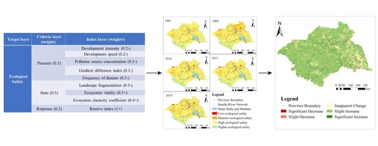
| Target Layer | Criterion Layer (Weight) | Parameter Layer (Weight ±) |
|---|---|---|
| Ecological safety (ES) | Pressure (P) (0.3) | Development intensity (0.2−) |
| Development speed (0.2−) | ||
| Pollution load (0.3−) | ||
| Gradient difference index (0.1−) | ||
| Frequency of disaster (0.2−) | ||
| State (S) (0.5) | Landscape fragmentation (0.3−) | |
| Ecosystem vitality (0.3+) | ||
| Ecosystem elasticity (0.4+) | ||
| Response (R) (0.2) | Reserve area index(1+) |
| Value | Level | Description |
|---|---|---|
| 0~0.2 | 1 | Lower ES, worse sustainable development ability |
| 0.2~0.4 | 2 | Low ES, poor sustainable development ability |
| 0.4~0.6 | 3 | Medium ES, medium sustainable development ability |
| 0.6~0.8 | 4 | High ES, good sustainable development ability |
| 0.8~1 | 5 | Higher ES, better sustainable development ability |
| Data Type | Attributes | Acquisition Dates | Sources |
|---|---|---|---|
| Nighttime light data | satellite data | 2001–2019 | https://www.ngdc.noaa.gov/eog/dmsp/downloadV4composites.html http://satsee.radi.ac.cn/cfimage/nightlight/ (accessed on 2 January 2021) |
| Precipitation | satellite data | 2001–2019 | National Earth System Science Data Center (http://www.geodata.cn (accessed on 10 November 2020)) |
| Surface temperature | satellite data | 2001–2019 | |
| Digital elevation model (DEM) | satellite data | - | Geospatial Data Cloud (http://www.gscloud.cn/ (accessed on 10 November 2020)) |
| MOD13Q1 NDVI | satellite data | 2001–2019 | NASA LAADS DAAC (https://ladsweb.modaps.eosdis.nasa.gov/search (accessed on 30 November 2020)) |
| MCD12Q1Land Cover Type | satellite data | 2001–2019 | NASA LAADS DAAC (https://ladsweb.modaps.eosdis.nasa.gov/search (accessed on 30 November 2020)) |
| Basin boundary | geospatial data | - | Resource and Environment Data Cloud Platform (http://www.resdc.cn/Default.aspx (accessed on 1 November 2020)) |
| Country boundary | geospatial data | - | Resource and Environment Data Cloud Platform (http://www.resdc.cn/Default.aspx (accessed on 10 November 2020)) |
| Reserve area | geospatial data | - | World Database on Protected Areas (https://www.protectedplanet.net/?from=singlemessage&isappinstalled=0 (accessed on 10 November 2020)) |
| Statistical data | other | 2001–2019 | Information Center of the Ministry of Water Resources of Chinahttp://xxzx.mwr.gov.cn/xxgk/gbjb/sqnb/ (accessed on 10 November 2020) Hydrology Bureau of the Huaihe River Water Conservancy Committee http://www.hrc.gov.cn/swj/szygb/24350.jhtml (accessed on 10 December 2020) |
| Policy information | other | 2001–2019 | The People’s Government of Jiangsu Province (http://en.jiangsu.gov.cn/ (accessed on 10 March 2021)) The People’s Government of Anhui Province (http://english.ah.gov.cn/ (accessed on 10 March 2021)) The People’s Government of Henan Province (http://english.henan.gov.cn/ (accessed on 10 March 2021)) The People’s Government of Shandong Province (http://www.shandong.gov.cn/index.html (accessed on 10 March 2021)) |
| Value | Description |
|---|---|
| −0.0191 to −0.0069 | Significant Decrease |
| −0.0069 to −0.0022 | Slight Decrease |
| −0.0022 to 0.0004 | Inapparent Change |
| 0.0004 to 0.0011 | Slight Increase |
| 0.0011 to 0.0124 | Significant Increase |
Publisher’s Note: MDPI stays neutral with regard to jurisdictional claims in published maps and institutional affiliations. |
© 2021 by the authors. Licensee MDPI, Basel, Switzerland. This article is an open access article distributed under the terms and conditions of the Creative Commons Attribution (CC BY) license (https://creativecommons.org/licenses/by/4.0/).
Share and Cite
Sang, S.; Wu, T.; Wang, S.; Yang, Y.; Liu, Y.; Li, M.; Zhao, Y. Ecological Safety Assessment and Analysis of Regional Spatiotemporal Differences Based on Earth Observation Satellite Data in Support of SDGs: The Case of the Huaihe River Basin. Remote Sens. 2021, 13, 3942. https://0-doi-org.brum.beds.ac.uk/10.3390/rs13193942
Sang S, Wu T, Wang S, Yang Y, Liu Y, Li M, Zhao Y. Ecological Safety Assessment and Analysis of Regional Spatiotemporal Differences Based on Earth Observation Satellite Data in Support of SDGs: The Case of the Huaihe River Basin. Remote Sensing. 2021; 13(19):3942. https://0-doi-org.brum.beds.ac.uk/10.3390/rs13193942
Chicago/Turabian StyleSang, Shan, Taixia Wu, Shudong Wang, Yingying Yang, Yiyao Liu, Mengyao Li, and Yuting Zhao. 2021. "Ecological Safety Assessment and Analysis of Regional Spatiotemporal Differences Based on Earth Observation Satellite Data in Support of SDGs: The Case of the Huaihe River Basin" Remote Sensing 13, no. 19: 3942. https://0-doi-org.brum.beds.ac.uk/10.3390/rs13193942