
Incorporating Multi-Scale, Spectrally Detected Nitrogen Concentrations into Assessing Nitrogen Use Efficiency for Winter Wheat Breeding Populations

 , and
, and
Abstract
:1. Introduction
2. Materials and Methods
2.1. Experimental Design
2.2. Spectral and Reference Tissue Collections
2.2.1. Data Collection 2017
2.2.2. Data Collection 2018
2.3. Standard Nitrogen Analysis
2.4. Chemometric Modeling
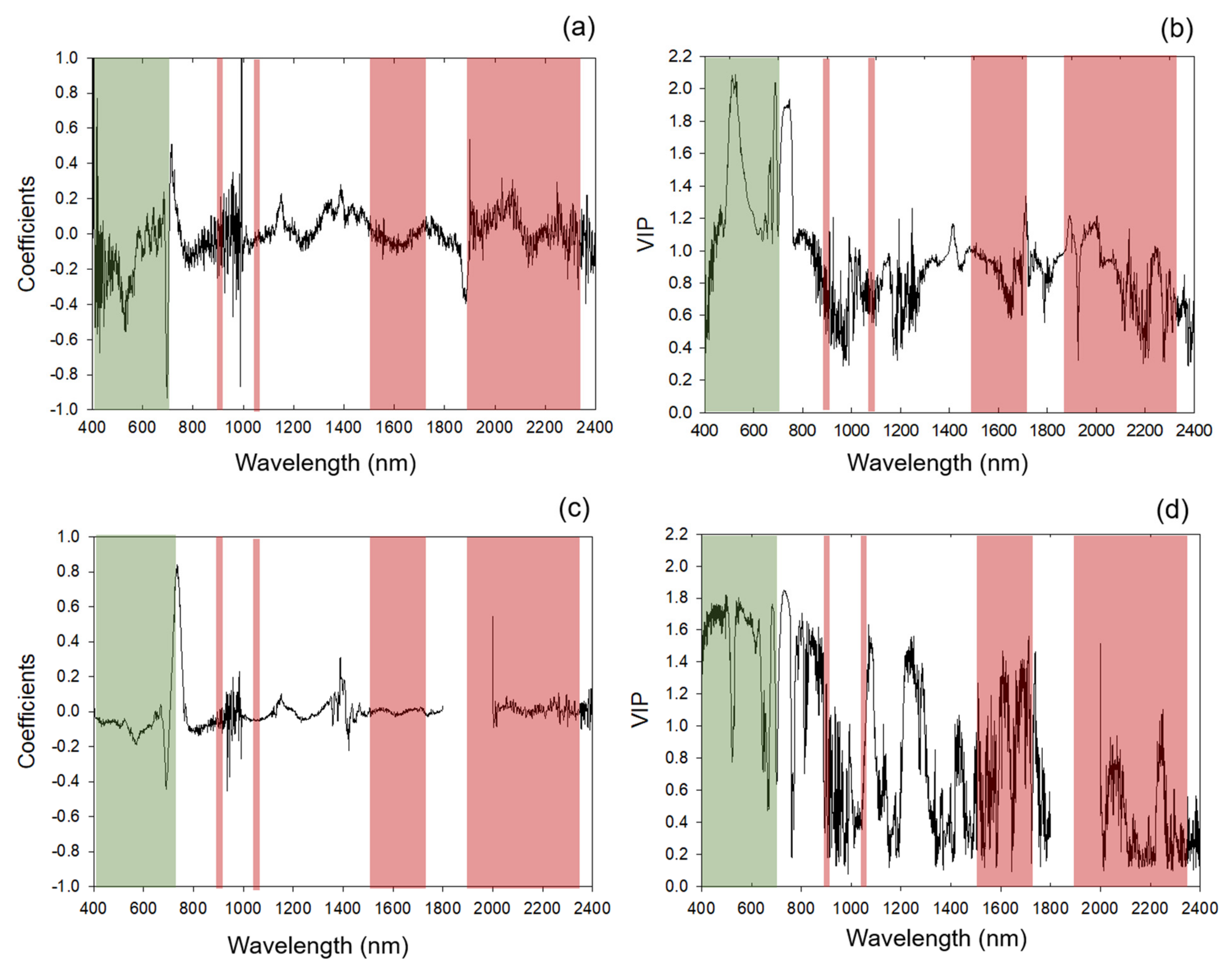
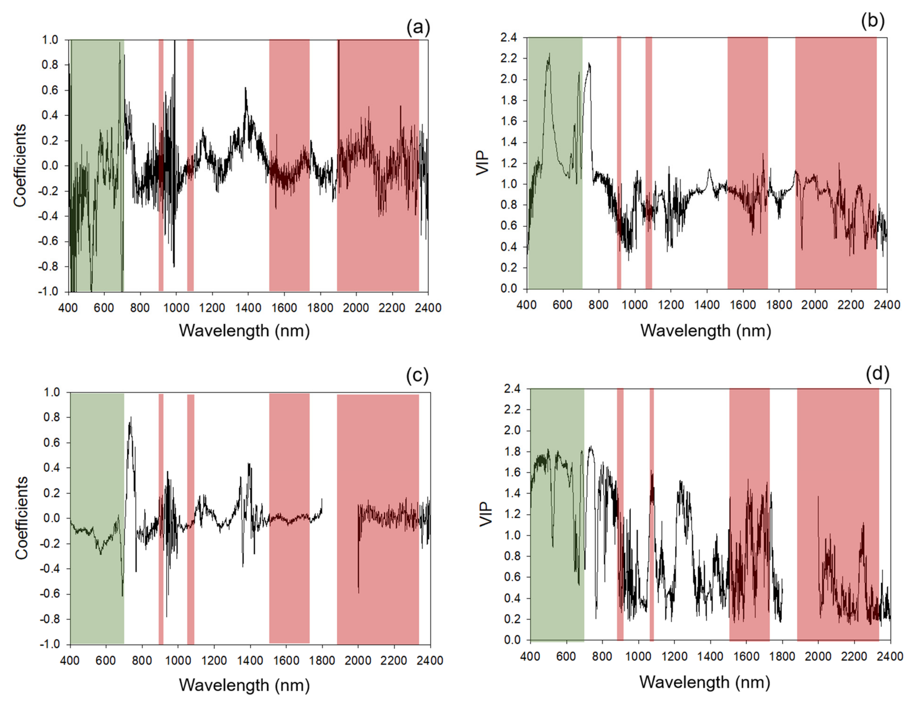
Categorization of Standardized Coefficients and VIP within Regions of Chlorophyll and Protein Absorption Features
2.5. NUE Quantification
3. Results
3.1. Chemometric Models
3.1.1. Modeling and Cross-Year Validation 2017
3.1.2. Multi-Year Models: Combining 2017 and 2018 Datasets
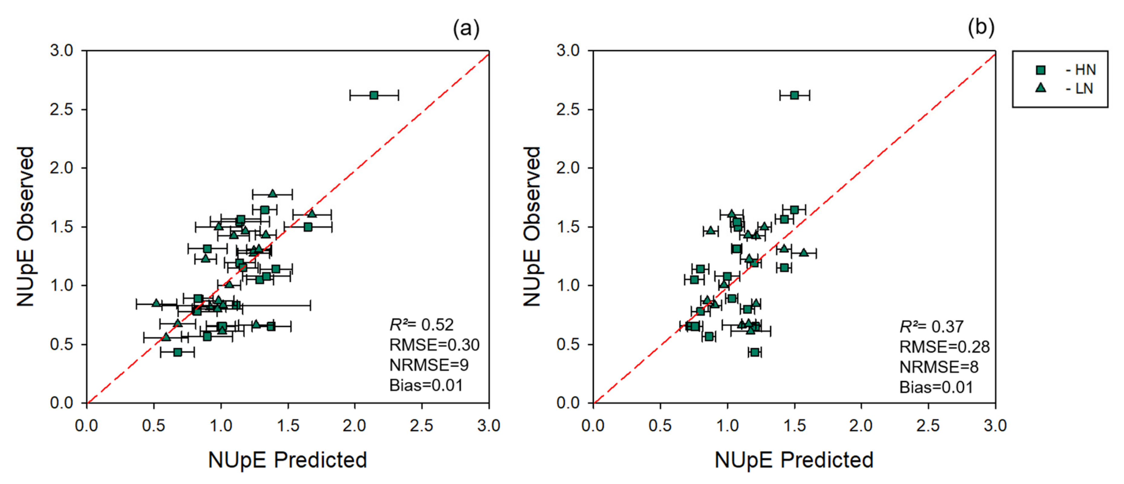
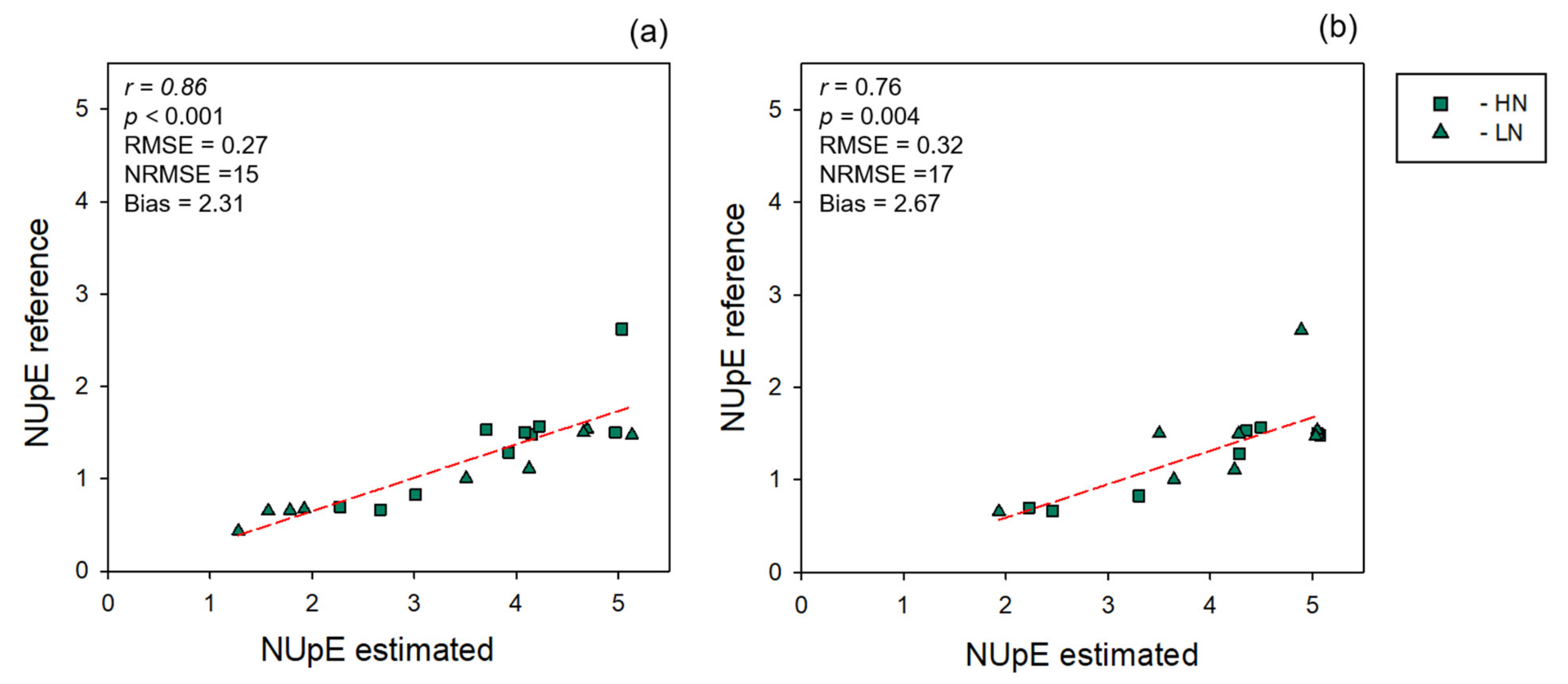
3.2. NUE Prediction
4. Discussion
5. Conclusions
Author Contributions
Funding
Acknowledgments
Conflicts of Interest
Appendix A

| Components | Plot 5 North | Plot 5 South |
|---|---|---|
| Phosphorus (Bray P1lbs/acre) | 43 | 53 |
| Potassium (pounds/acre) | 195 | 188 |
| Calcium (pounds/acre) | 2326 | 2214 |
| Magnesium (pounds/acre) | 715 | 621 |
| Base Sat’n (%) | 97 | 100 |
| Calcium Sat’n (%) | 62 | 66 |
| Ca/Mg Ratio | 2 | 2.2 |
| CEC (meq/100 g) | 11.09 | 9.95 |
| Potassium Sat’n (%) | 2.52 | 2.71 |
| Magnesium Sat’n (%) | 31 | 30 |
| Mg/K Ratio | 12.5 | 11.2 |
| pH | 6.93 | 7 |
| Lime Index | 69.73 | 70 |
Appendix B
| Dataset | Wheat Line ID (Purdue ID) |
|---|---|
| 2017 | 04606RA1-7-1-4 (PU01) |
| 053A1-2-5-3-5 (PU02) | |
| 10101RA1-6-2 (PU26) | |
| 11407A1-6 (PU24) | |
| 2018 | 0175A1-31-4-1 (PU17) |
| 03549A1-18-25-4 (PU05) | |
| 04606RA1-7-1 (PU07) | |
| 04606RA1-7-1-4 (PU01) | |
| 04606RA1-7-1-6 (PU23) | |
| 04719A1-16-1-1-47-4 (PU19) | |
| 05247A1-7-3-29 (PU10) | |
| 05247A1-7-3-98 (PU08) | |
| 05247A-7-7-3-1 (PU25) | |
| 05251A1-1-77-16-3 (PU22) | |
| 0537A1-3-12-1 (PU14) | |
| 053A1-2-5-3-5-3 (PU02) | |
| 0566A1-3-1-48 (PU09) | |
| 0570A1-2-39-2-4 (PU06) | |
| 0570A1-8-5-1 (PU03) | |
| 057RA1-8-5-3 (PU13) | |
| 057RA1-8-5-33 (PU11) | |
| 06497A1-7-3 (PU21) | |
| 07117B1-29-7-9-9-4-3-6-3 (PU29) | |
| 0722A1-1-1-7 (PU04) | |
| 07469A1-6-1-1 (PU18) | |
| 0762A1-2-8 (PU15) | |
| 08334A1-31 (PU12) | |
| 10101RA1-6-2 (PU26) | |
| 10221A1-8-1 (PU27) | |
| 10222A1-9-2 (PU30) | |
| 1041RB1-10 (PU16) | |
| 10447A1-5 (PU28) | |
| 10565C1-1 (PU20) | |
| 11407A1-6 (PU24) | |
| CHECK—P25R40 | |
| CHECK—P25R62 |
Appendix C
| Chemical | WL Highest Peak | Absorption Mechanisms | Literature Described the WL |
|---|---|---|---|
| Chlorophyll a | 420 | Electron transition | Kumar et al., 2005 |
| Chlorophyll a | 430 | Electron transition | Curran et al., 1989 |
| Chlorophyll b | 435 | Electron transition | Kumar et al., 2005 |
| Chlorophyll b | 460 | Electron transition | Curran et al., 1989 |
| Chlorophyll a | 490 | Electron transition | Kumar et al., 2005 |
| Chlorophyll | 530 | Electron transition | Curran et al., 2001 |
| Chlorophyll a | 550 | Electron transition | Datt et al., 1998 and Gitelson et al., 1995 |
| Chlorophyll | 630 | Electron transition | Curran et al., 2001 |
| Chlorophyll b | 640 | Electron transition | Curran et al., 1989 |
| Chlorophyll b | 643 | Electron transition | Kumar et al., |
| Chlorophyll a | 660 | Electron transition | Curran et al., 1989; Kumar et al., 2005 |
| Chlorophyll | 675 | Electron transition | Datt et al., 1998 |
| Chlorophyll | 700 | Not described | Curran et al., 2001; Gitelson et al., 1995 |
| Protein | 910 | C-H stretch, 3rd overtone | Curran et al., 1989 |
| Protein | 1020 | N-H stretch | Curran et al., 1989 |
| Protein | 1500 | Not described | Kumar et al., 2005 |
| Protein | 1510 | N-H stretch, 1st overtone | Curran et al., 1989 |
| Protein | 1520 | N-H stretch, 1st overtone | Berger et al., 2020 |
| Protein | 1680 | C-H strecth, 1st overtone | Kumar et al., 2005 |
| Protein | 1690 | C-H strecth, 1st overtone | Berger et al., 2020 |
| Protein | 1730 | C-H stretch | Kumar et al., 2005 |
| Protein | 1940 | O-H strech, O-H deformation | Curran et al., 1989; Kumar et al., 2005 |
| Protein | 1960 | N-H assymmetry | Berger et al., 2020 |
| Protein | 1980 | N-H assymmetry | Curran et al., 1989 |
| Protein | 2050 | N-H stretch, N=H rotation | Kumar et al., 2005 |
| Protein | 2060 | N-H stretch, N=H rotation | Curran et al., 1989 |
| Protein | 2130 | N-H stretch | Curran et al., 1989 |
| Protein | 2170 | Not described | Kumar et al., 2005 |
| Protein | 2180 | N-H rotation, C-H stretch, C-O stretch, C=O stretch | Curran et al., 1989 |
| Protein | 2200 | N-H rotation, C-H stretch, C-O stretch, C=O stretch | Berger et al., 2020 |
| Protein | 2240 | C-H stretch | Curran et al., 1989 |
| Protein | 2270 | C-H stretch | Berger et al., 2020 |
| Protein | 2290 | C-H rotation, C=O stretch, N-H stretch | Kumar et al., 2005 |
| Protein | 2300 | C-H rotation, C=O stretch, N-H stretch | Curran et al., 1989 |
| Protein | 2350 | CH2 rotation, C-H deformation | Curran et al., 1989 |
Appendix D
| 2017 Models | Multi-Year Models | ||||
|---|---|---|---|---|---|
| WL Highest Peak | Chemical | Leaf Level | Canopy Level | Leaf Level | Canopy Level |
| 420 | Chlorophyll a | 0.42 | 0.09 | 0.69 | 0.09 |
| 430 | Chlorophyll a | 0.29 | 0.05 | 0.59 | 0.08 |
| 435 | Chlorophyll b | 0.26 | 0.05 | 0.57 | 0.09 |
| 460 | Chlorophyll b | 0.2 | 0.05 | 0.33 | 0.09 |
| 490 | Chlorophyll a | 0.19 | 0.06 | 0.21 | 0.10 |
| 530 | Chlorophyll | 0.37 | 0.08 | 0.58 | 0.13 |
| 550 | Chlorophyll a | 0.31 | 0.12 | 0.38 | 0.20 |
| 630 | Chlorophyll | 0.05 | 0.06 | 0.10 | 0.13 |
| 640 | Chlorophyll b | 0.06 | 0.05 | 0.13 | 0.11 |
| 643 | Chlorophyll b | 0.06 | 0.04 | 0.13 | 0.10 |
| 660 | Chlorophyll a | 0.06 | 0.03 | 0.15 | 0.07 |
| 675 | Chlorophyll | 0.14 | 0.14 | 0.31 | 0.21 |
| 700 | Chlorophyll | 0.38 | 0.25 | 0.58 | 0.32 |
| 910 | Protein | 0.1 | 0.05 | 0.15 | 0.11 |
| 1020 | Protein | 0.05 | 0.04 | 0.13 | 0.06 |
| 1500 | Protein | 0.05 | 0.01 | 0.05 | 0.02 |
| 1510 | Protein | 0.03 | 0.01 | 0.05 | 0.02 |
| 1520 | Protein | 0.03 | 0.01 | 0.04 | 0.01 |
| 1680 | Protein | 0.02 | 0.01 | 0.05 | 0.01 |
| 1690 | Protein | 0.02 | 0.01 | 0.05 | 0.01 |
| 1730 | Protein | 0.04 | 0.01 | 0.06 | 0.01 |
| 1940 | Protein | 0.05 | NA | 0.08 | NA |
| 1960 | Protein | 0.06 | NA | 0.10 | NA |
| 1980 | Protein | 0.07 | NA | 0.11 | NA |
| 2050 | Protein | 0.16 | 0.03 | 0.17 | 0.05 |
| 2060 | Protein | 0.17 | 0.03 | 0.20 | 0.05 |
| 2130 | Protein | 0.07 | 0.01 | 0.18 | 0.02 |
| 2170 | Protein | 0.05 | 0.01 | 0.12 | 0.04 |
| 2180 | Protein | 0.03 | 0.01 | 0.10 | 0.03 |
| 2200 | Protein | 0.03 | 0.01 | 0.07 | 0.03 |
| 2240 | Protein | 0.08 | 0.03 | 0.14 | 0.05 |
| 2270 | Protein | 0.08 | 0.03 | 0.14 | 0.04 |
| 2290 | Protein | 0.08 | 0.03 | 0.15 | 0.04 |
| 2300 | Protein | 0.09 | 0.03 | 0.14 | 0.04 |
| 2350 | Protein | 0.13 | 0.03 | 0.15 | 0.05 |
| 2017 Models | Multi-Year Models | ||||
|---|---|---|---|---|---|
| Wavelength (nm) | Chemicall | Leaf Level | Canopy Level | Leaf Level | Canopy Level |
| 420 | Chlorophyll a | 0.8 | 1.6 | 0.8 | 1.6 |
| 430 | Chlorophyll a | 0.9 | 1.6 | 0.9 | 1.6 |
| 435 | Chlorophyll b | 1.0 | 1.7 | 1.0 | 1.7 |
| 460 | Chlorophyll b | 1.1 | 1.7 | 1.1 | 1.7 |
| 490 | Chlorophyll a | 1.5 | 1.7 | 1.5 | 1.7 |
| 530 | Chlorophyll | 1.9 | 1.4 | 1.9 | 1.4 |
| 550 | Chlorophyll a | 1.6 | 1.7 | 1.6 | 1.7 |
| 630 | Chlorophyll | 1.1 | 1.4 | 1.4 | 1.4 |
| 640 | Chlorophyll b | 1.1 | 1.2 | 1.2 | 1.2 |
| 643 | Chlorophyll b | 1.2 | 1.2 | 1.2 | 1.2 |
| 660 | Chlorophyll a | 1.3 | 1.0 | 1.3 | 0.9 |
| 675 | Chlorophyll | 1.5 | 1.2 | 1.5 | 1.2 |
| 700 | Chlorophyll | 1.6 | 1.4 | 1.6 | 1.4 |
| 910 | Protein | 0.7 | 0.6 | 0.7 | 0.7 |
| 1020 | Protein | 0.8 | 0.4 | 0.9 | 0.4 |
| 1500 | Protein | 1.0 | 0.6 | 1.0 | 0.7 |
| 1510 | Protein | 1.0 | 0.6 | 1.0 | 0.7 |
| 1520 | Protein | 1.0 | 0.6 | 1.0 | 0.6 |
| 1680 | Protein | 0.9 | 1.1 | 0.9 | 1.1 |
| 1690 | Protein | 0.9 | 1.2 | 0.9 | 1.1 |
| 1730 | Protein | 1.0 | 0.9 | 1.0 | 0.9 |
| 1940 | Protein | 0.9 | NA | 0.9 | NA |
| 1960 | Protein | 1.1 | NA | 1.0 | NA |
| 1980 | Protein | 1.1 | NA | 1.0 | NA |
| 2050 | Protein | 0.9 | 0.7 | 0.9 | 0.7 |
| 2060 | Protein | 0.9 | 0.7 | 1.0 | 0.7 |
| 2130 | Protein | 0.8 | 0.3 | 0.8 | 0.4 |
| 2170 | Protein | 0.6 | 0.2 | 0.7 | 0.3 |
| 2180 | Protein | 0.6 | 0.2 | 0.6 | 0.3 |
| 2200 | Protein | 0.5 | 0.2 | 0.6 | 0.3 |
| 2240 | Protein | 0.9 | 0.7 | 0.9 | 0.8 |
| 2270 | Protein | 0.7 | 0.4 | 0.7 | 0.4 |
| 2290 | Protein | 0.6 | 0.3 | 0.6 | 0.3 |
| 2300 | Protein | 0.7 | 0.3 | 0.6 | 0.3 |
| 2350 | Protein | 0.7 | 0.3 | 0.6 | 0.3 |
| 2017 Models | |||||||
|---|---|---|---|---|---|---|---|
| Leaf Level | Canopy Level | ||||||
| WL Range (nm) | Coefficient | WL Range (nm) | Coefficient | ||||
| 400 | - | 429 | 0.51 | 400 | - | 429 | 0.10 |
| 430 | - | 459 | 0.21 | 430 | - | 459 | 0.06 |
| 460 | - | 489 | 0.18 | 460 | - | 489 | 0.06 |
| 490 | - | 519 | 0.23 | 490 | - | 519 | 0.07 |
| 520 | - | 549 | 0.40 | 520 | - | 549 | 0.08 |
| 550 | - | 579 | 0.21 | 550 | - | 579 | 0.16 |
| 670 | - | 699 | 0.28 | 580 | - | 609 | 0.12 |
| 700 | - | 729 | 0.33 | 610 | - | 639 | 0.08 |
| 760 | - | 789 | 0.12 | 670 | - | 699 | 0.22 |
| 790 | - | 819 | 0.12 | 700 | - | 729 | 0.34 |
| 910 | - | 939 | 0.13 | 730 | - | 759 | 0.57 |
| 940 | - | 969 | 0.14 | 760 | - | 789 | 0.07 |
| 970 | - | 999 | 0.41 | 790 | - | 819 | 0.11 |
| 1120 | - | 1149 | 0.09 | 820 | - | 849 | 0.09 |
| 1300 | - | 1329 | 0.11 | 850 | - | 879 | 0.08 |
| 1330 | - | 1359 | 0.15 | 880 | - | 909 | 0.05 |
| 1360 | - | 1389 | 0.16 | 910 | - | 939 | 0.08 |
| 1390 | - | 1419 | 0.13 | 940 | - | 969 | 0.08 |
| 1420 | - | 1449 | 0.13 | 970 | - | 999 | 0.06 |
| 1450 | - | 1479 | 0.11 | 1000 | - | 1029 | 0.04 |
| 1870 | - | 1899 | 0.28 | 1030 | - | 1059 | 0.05 |
| 1900 | - | 1929 | 0.11 | 1060 | - | 1089 | 0.04 |
| 1990 | - | 2019 | 0.11 | 1120 | - | 1149 | 0.04 |
| 2020 | - | 2049 | 0.14 | 1150 | - | 1179 | 0.04 |
| 2050 | - | 2079 | 0.18 | 1240 | - | 1269 | 0.04 |
| 2230 | - | 2259 | 0.09 | 1330 | - | 1359 | 0.05 |
| 2290 | - | 2319 | 0.09 | 1360 | - | 1389 | 0.08 |
| 2320 | - | 2349 | 0.12 | 1390 | - | 1419 | 0.14 |
| 2350 | - | 2379 | 0.11 | 1420 | - | 1449 | 0.07 |
| 2380 | - | 2400 | 0.13 | 2370 | - | 2400 | 0.05 |
| 2017 Model | Multi-Year Models | ||||||||||||||
|---|---|---|---|---|---|---|---|---|---|---|---|---|---|---|---|
| Leaf Level | Canopy Level | Leaf Level | Canopy Level | ||||||||||||
| WL Range (nm) | VIP ≥ 0.8 | WL Range (nm) | VIP ≥ 0.8 | WL Range (nm) | VIP ≥ 0.8 | WL Range (nm) | VIP ≥ 0.8 | ||||||||
| 430 | - | 459 | 1.1 | 400 | - | 429 | 1.6 | 430 | - | 459 | 1.1 | 400 | - | 429 | 1.5 |
| 460 | - | 489 | 1.2 | 430 | - | 459 | 1.7 | 460 | - | 489 | 1.2 | 430 | - | 459 | 1.7 |
| 490 | - | 519 | 1.9 | 460 | - | 489 | 1.7 | 490 | - | 519 | 1.9 | 460 | - | 489 | 1.7 |
| 520 | - | 549 | 1.9 | 490 | - | 519 | 1.6 | 520 | - | 549 | 1.9 | 490 | - | 519 | 1.6 |
| 550 | - | 579 | 1.4 | 520 | - | 549 | 1.4 | 550 | - | 579 | 1.3 | 520 | - | 549 | 1.4 |
| 580 | - | 609 | 1.2 | 550 | - | 579 | 1.7 | 580 | - | 609 | 1.2 | 550 | - | 579 | 1.7 |
| 610 | - | 639 | 1.1 | 580 | - | 609 | 1.6 | 610 | - | 639 | 1.1 | 580 | - | 609 | 1.7 |
| 640 | - | 669 | 1.3 | 610 | - | 639 | 1.5 | 640 | - | 669 | 1.3 | 610 | - | 639 | 1.5 |
| 670 | - | 699 | 1.6 | 640 | - | 669 | 0.9 | 670 | - | 699 | 1.6 | 640 | - | 669 | 0.8 |
| 700 | - | 729 | 1.7 | 670 | - | 699 | 1.4 | 700 | - | 729 | 1.7 | 670 | - | 699 | 1.4 |
| 730 | - | 759 | 1.8 | 700 | - | 729 | 1.4 | 730 | - | 759 | 2.0 | 700 | - | 729 | 1.4 |
| 760 | - | 789 | 1.1 | 730 | - | 759 | 1.7 | 760 | - | 789 | 1.1 | 730 | - | 759 | 1.7 |
| 790 | - | 819 | 1.1 | 760 | - | 789 | 1.0 | 790 | - | 819 | 1.1 | 760 | - | 789 | 1.0 |
| 820 | - | 849 | 1.0 | 790 | - | 819 | 1.4 | 820 | - | 849 | 1.0 | 790 | - | 819 | 1.4 |
| 850 | - | 879 | 0.9 | 820 | - | 849 | 1.5 | 850 | - | 879 | 0.9 | 820 | - | 849 | 1.5 |
| 1000 | - | 1029 | 0.8 | 850 | - | 879 | 1.4 | 1000 | - | 1029 | 0.9 | 850 | - | 879 | 1.3 |
| 1030 | - | 1059 | 0.8 | 880 | - | 909 | 0.8 | 1030 | - | 1059 | 0.8 | 880 | - | 909 | 0.8 |
| 1120 | - | 1149 | 0.9 | 1060 | - | 1089 | 1.4 | 1090 | - | 1119 | 0.8 | 1060 | - | 1089 | 1.4 |
| 1270 | - | 1299 | 0.8 | 1210 | - | 1239 | 1.4 | 1120 | - | 1149 | 0.9 | 1210 | - | 1239 | 1.4 |
| 1300 | - | 1329 | 0.9 | 1240 | - | 1269 | 1.3 | 1210 | - | 1239 | 0.8 | 1240 | - | 1269 | 1.2 |
| 1330 | - | 1359 | 0.9 | 1270 | - | 1299 | 1.1 | 1270 | - | 1299 | 0.8 | 1270 | - | 1299 | 1.2 |
| 1360 | - | 1389 | 0.9 | 1420 | - | 1449 | 0.8 | 1300 | - | 1329 | 0.9 | 1420 | - | 1449 | 0.8 |
| 1390 | - | 1419 | 1.1 | 1600 | - | 1629 | 1.2 | 1330 | - | 1359 | 0.9 | 1600 | - | 1629 | 1.2 |
| 1420 | - | 1449 | 1.0 | 1660 | - | 1689 | 1.2 | 1360 | - | 1389 | 0.9 | 1660 | - | 1689 | 1.1 |
| 1450 | - | 1479 | 1.0 | 1690 | - | 1719 | 1.1 | 1390 | - | 1419 | 1.1 | 1690 | - | 1719 | 1.1 |
| 1480 | - | 1509 | 1.0 | 1720 | - | 1749 | 0.9 | 1420 | - | 1449 | 1.0 | 1720 | - | 1749 | 0.9 |
| 1510 | - | 1539 | 1.0 | 1450 | - | 1479 | 0.9 | 2040 | - | 2069 | 0.8 | ||||
| 1540 | - | 1569 | 0.9 | 1480 | - | 1509 | 1.0 | 2220 | - | 2249 | 0.8 | ||||
| 1570 | - | 1599 | 0.9 | 1510 | - | 1539 | 0.9 | ||||||||
| 1600 | - | 1629 | 0.8 | 1540 | - | 1569 | 0.9 | ||||||||
| 1660 | - | 1689 | 0.9 | 1570 | - | 1599 | 0.9 | ||||||||
| 1690 | - | 1719 | 1.1 | 1600 | - | 1629 | 0.9 | ||||||||
| 1720 | - | 1749 | 0.9 | 1660 | - | 1689 | 0.9 | ||||||||
| 1750 | - | 1779 | 0.9 | 1690 | - | 1719 | 1.0 | ||||||||
| 1780 | - | 1809 | 0.8 | 1720 | - | 1749 | 0.9 | ||||||||
| 1810 | - | 1839 | 0.9 | 1750 | - | 1779 | 0.9 | ||||||||
| 1840 | - | 1869 | 1.0 | 1780 | - | 1809 | 0.8 | ||||||||
| 1870 | - | 1899 | 1.1 | 1810 | - | 1839 | 0.9 | ||||||||
| 1900 | - | 1929 | 0.9 | 1840 | - | 1869 | 0.9 | ||||||||
| 1930 | - | 1959 | 1.0 | 1870 | - | 1899 | 1.1 | ||||||||
| 1960 | - | 1989 | 1.1 | 1900 | - | 1929 | 0.9 | ||||||||
| 1990 | - | 2019 | 1.1 | 1930 | - | 1959 | 1.0 | ||||||||
| 2020 | - | 2049 | 0.9 | 1960 | - | 1989 | 1.0 | ||||||||
| 2050 | - | 2079 | 0.9 | 1990 | - | 2019 | 1.0 | ||||||||
| 2080 | - | 2109 | 0.8 | 2020 | - | 2049 | 0.9 | ||||||||
| 2110 | - | 2139 | 0.8 | 2050 | - | 2079 | 1.0 | ||||||||
| 2230 | - | 2259 | 1.0 | 2080 | - | 2109 | 0.8 | ||||||||
| 2110 | - | 2139 | 0.8 | ||||||||||||
| 2140 | - | 2169 | 0.8 | ||||||||||||
| 2230 | - | 2259 | 0.9 | ||||||||||||
| Multi-Year Models | |||||||
|---|---|---|---|---|---|---|---|
| Leaf Level | Canopy Level | ||||||
| WL Range (nm) | Coefficient | WL Range (nm) | Coefficient | ||||
| 400 | - | 429 | 0.77 | 400 | - | 429 | 0.10 |
| 430 | - | 459 | 0.45 | 430 | - | 459 | 0.10 |
| 460 | - | 489 | 0.23 | 460 | - | 489 | 0.09 |
| 490 | - | 519 | 0.25 | 490 | - | 519 | 0.11 |
| 520 | - | 549 | 0.64 | 520 | - | 549 | 0.14 |
| 550 | - | 579 | 0.23 | 550 | - | 579 | 0.24 |
| 640 | - | 669 | 0.16 | 580 | - | 609 | 0.20 |
| 670 | - | 699 | 0.52 | 610 | - | 639 | 0.15 |
| 700 | - | 729 | 0.40 | 670 | - | 699 | 0.31 |
| 730 | - | 759 | 0.26 | 700 | - | 729 | 0.35 |
| 760 | - | 789 | 0.15 | 730 | - | 759 | 0.54 |
| 790 | - | 819 | 0.17 | 760 | - | 789 | 0.18 |
| 910 | - | 939 | 0.18 | 790 | - | 819 | 0.11 |
| 940 | - | 969 | 0.24 | 820 | - | 849 | 0.13 |
| 970 | - | 999 | 0.51 | 850 | - | 879 | 0.08 |
| 1000 | - | 1029 | 0.15 | 880 | - | 909 | 0.07 |
| 1300 | - | 1329 | 0.16 | 910 | - | 939 | 0.17 |
| 1330 | - | 1359 | 0.18 | 940 | - | 969 | 0.18 |
| 1360 | - | 1389 | 0.30 | 970 | - | 999 | 0.12 |
| 1390 | - | 1419 | 0.33 | 1030 | - | 1059 | 0.07 |
| 1420 | - | 1449 | 0.27 | 1090 | - | 1119 | 0.08 |
| 1450 | - | 1479 | 0.15 | 1120 | - | 1149 | 0.07 |
| 1870 | - | 1899 | 0.15 | 1150 | - | 1179 | 0.07 |
| 1900 | - | 1929 | 0.28 | 1330 | - | 1359 | 0.20 |
| 2050 | - | 2079 | 0.22 | 1360 | - | 1389 | 0.14 |
| 2110 | - | 2139 | 0.17 | 1390 | - | 1419 | 0.21 |
| 2140 | - | 2169 | 0.19 | 1420 | - | 1449 | 0.08 |
| 2230 | - | 2259 | 0.16 | 1780 | - | 2009 | 0.08 |
| 2350 | - | 2379 | 0.16 | 2340 | - | 2369 | 0.07 |
| 2380 | - | 2400 | 0.19 | 2370 | - | 2400 | 0.09 |
References
- Shiferaw, B.; Smale, M.; Braun, H.-J.; Duveiller, E.; Reynolds, M.; Muricho, G. Crops that feed the world Past successes and future challenges to the role played by wheat in global food security. Food Secur. 2013, 5, 291–317. [Google Scholar] [CrossRef] [Green Version]
- FAO. GIEWS Crop Prospects and Food Situation. 2 July 2019. Available online: http://www.fao.org/documents/card/en/c/ca5327en (accessed on 15 January 2020).
- Phillips, B.S.; Norton, R. Global Wheat Production and Fertilizer Use. Better Crop. 2012, 96, 4–6. [Google Scholar]
- Rose, G.J. Crop Production. Soil Sci. 1956, 81, 152. [Google Scholar] [CrossRef]
- Li, G.; Yu, M.; Fang, T.; Cao, S.; Carver, B.F.; Yan, L. Vernalization requirement duration in winter wheat is controlled by T a VRN—A 1 at the protein level. Plant J. 2013, 76, 742–753. [Google Scholar] [CrossRef] [PubMed] [Green Version]
- Dong, K.; Zhen, S.; Cheng, Z.; Cao, H.; Ge, P.; Yan, Y. Proteomic Analysis Reveals Key Proteins and Phosphoproteins upon Seed Germination of Wheat (Triticum aestivum L.). Front. Plant Sci. 2015, 6. [Google Scholar] [CrossRef] [PubMed] [Green Version]
- Delogu, G.; Cattivelli, L.; Pecchioni, N.; De Falcis, D.; Maggiore, T.; Stanca, A. Uptake and agronomic efficiency of nitrogen in winter barley and winter wheat. Eur. J. Agron. 1998, 9, 11–20. [Google Scholar] [CrossRef]
- Barbottin, A.; LeComte, C.; Bouchard, C.; Jeuffroy, M.-H. Nitrogen Remobilization during Grain Filling in Wheat: Genotypic and Environmental Effects. Crop. Sci. 2005, 45, 1141–1150. [Google Scholar] [CrossRef]
- Robertson, G.; Vitousek, P.M. Nitrogen in Agriculture: Balancing the Cost of an Essential Resource. Annu. Rev. Environ. Resour. 2009, 34, 97–125. [Google Scholar] [CrossRef] [Green Version]
- Garnett, T.; Plett, D.; Heuer, S.; Okamoto, M. Genetic approaches to enhancing nitrogen-use efficiency (NUE) in cereals: Challenges and future directions. Funct. Plant Biol. 2015, 42, 921. [Google Scholar] [CrossRef]
- Heisey, P.W.; Norton, G. Fertilizers and other farm chemicals. In Handbook of Agricultural Economics; Evenson, R., Pingali, P., Eds.; Elsevier North Holland: Amsterdam, The Netherlands, 2007; Volume 3, pp. 2741–2777. [Google Scholar]
- Wei, F.; Yan, Z.; Yongchao, T.; Weixing, C.; Xia, Y.; Yingxue, L. Monitoring leaf nitrogen accumulation in wheat with hyper-spectral remote sensing. Acta Ecol. Sin. 2008, 28, 23–32. [Google Scholar] [CrossRef]
- Hitz, K.; Clark, A.J.; Van Sanford, D.A. Identifying nitrogen-use efficient soft red winter wheat lines in high and low nitrogen environments. Field Crop. Res. 2017, 200, 1–9. [Google Scholar] [CrossRef] [Green Version]
- Moll, R.H.; Kamprath, E.J.; Jackson, W.A. Analysis and interpretation of factors which contribute to efficiency of nitrogen-utilization. Agron. J. 1982, 74, 562–564. [Google Scholar] [CrossRef]
- Kong, L.; Xie, Y.; Hu, L.; Feng, B.; Li, S. Remobilization of vegetative nitrogen to developing grain in wheat (Triticum aestivum L.). Field Crop. Res. 2016, 196, 134–144. [Google Scholar] [CrossRef]
- Han, M.; Okamoto, M.; Beatty, P.H.; Rothstein, S.J.; Good, A.G. The Genetics of Nitrogen Use Efficiency in Crop Plants. Annu. Rev. Genet. 2015, 49, 269–289. [Google Scholar] [CrossRef]
- Araus, J.L.; Kefauver, S.C.; Zaman-Allah, M.; Olsen, M.S.; Cairns, J. Translating High-Throughput Phenotyping into Genetic Gain. Trends Plant Sci. 2018, 23, 451–466. [Google Scholar] [CrossRef] [Green Version]
- Roitsch, T.; Cabrera-Bosquet, L.; Fournier, A.; Ghamkhar, K.; Jiménez-Berni, J.; Pinto, F.; Ober, E.S. Review: New sensors and data-driven approaches—A path to next generation phenomics. Plant Sci. 2019, 282, 2–10. [Google Scholar] [CrossRef]
- Curran, P.J. Remote sensing of foliar chemistry. Remote Sens. Environ. 1989, 30, 271–278. [Google Scholar] [CrossRef]
- Cotrozzi, L.; Townsend, P.A.; Pellegrini, E.; Nali, C.; Couture, J.J. Reflectance spectroscopy: A novel approach to better understand and monitor the impact of air pollution on Mediterranean plants. Environ. Sci. Pollut. Res. 2017, 25, 8249–8267. [Google Scholar] [CrossRef]
- Serbin, S.P.; Dillaway, D.N.; Kruger, E.L.; Townsend, P.A. Leaf optical properties reflect variation in photosynthetic metabolism and its sensitivity to temperature. J. Exp. Bot. 2011, 63, 489–502. [Google Scholar] [CrossRef] [PubMed] [Green Version]
- Li, F.; Mistele, B.; Hu, Y.; Chen, X.; Schmidhalter, U. Reflectance estimation of canopy nitrogen content in winter wheat using optimised hyperspectral spectral indices and partial least squares regression. Eur. J. Agron. 2014, 52, 198–209. [Google Scholar] [CrossRef]
- Féret, J.-B.; Berger, K.; de Boissieu, F.; Malenovský, Z. PROSPECT-PRO for estimating content of nitrogen-containing leaf proteins and other carbon-based constituents. Remote Sens. Environ. 2020, 252, 112173. [Google Scholar] [CrossRef]
- Ollinger, S.V. Sources of variability in canopy reflectance and the convergent properties of plants. New Phytol. 2010, 189, 375–394. [Google Scholar] [CrossRef]
- Couture, J.J.; Serbin, S.P.; Townsend, P.A. Spectroscopic sensitivity of real-time, rapidly induced phytochemical change in response to damage. New Phytol. 2013, 198, 311–319. [Google Scholar] [CrossRef]
- Serbin, S.P.; Singh, A.; Desai, A.R.; Dubois, S.G.; Jablonski, A.D.; Kingdon, C.; Kruger, E.L.; Townsend, P. Remotely estimating photosynthetic capacity, and its response to temperature, in vegetation canopies using imaging spectroscopy. Remote Sens. Environ. 2015, 167, 78–87. [Google Scholar] [CrossRef]
- Yuan, M.; Couture, J.J.; Townsend, P.A.; Ruark, M.D.; Bland, W.L. Spectroscopic Determination of Leaf Nitrogen Concentration and Mass Per Area in Sweet Corn and Snap Bean. Agron. J. 2016, 108, 2519–2526. [Google Scholar] [CrossRef]
- Cotrozzi, L.; Couture, J.J.; Cavender-Bares, J.; Kingdon, C.; Fallon, B.; Pilz, G.; Pellegrini, E.; Nali, C.; A Townsend, P. Using foliar spectral properties to assess the effects of drought on plant water potential. Tree Physiol. 2017, 37, 1582–1591. [Google Scholar] [CrossRef] [PubMed]
- Silva-Perez, V.; Molero, G.; Serbin, S.P.; Condon, A.G.; Reynolds, M.P.; Furbank, R.T.; Evans, J.R. Hyperspectral reflectance as a tool to measure biochemical and physiological traits in wheat. J. Exp. Bot. 2017, 69, 483–496. [Google Scholar] [CrossRef] [PubMed] [Green Version]
- Meacham-Hensold, K.; Montes, C.; Wu, J.; Guan, K.; Fu, P.; Ainsworth, E.A.; Pederson, T.; Moore, C.; Brown, K.L.; Raines, C.; et al. High-throughput field phenotyping using hyperspectral reflectance and partial least squares regression (PLSR) reveals genetic modifications to photosynthetic capacity. Remote Sens. Environ. 2019, 231, 111176. [Google Scholar] [CrossRef] [PubMed]
- Bruning, B.; Berger, B.; Lewis, M.; Liu, H.; Garnett, T. Approaches, applications, and future directions for hyperspectral vegetation studies: An emphasis on yield-limiting factors in wheat. Plant Phenome J. 2020, 3, 1–22. [Google Scholar] [CrossRef]
- Cotrozzi, L.; Peron, R.; Tuinstra, M.R.; Mickelbart, M.V.; Couture, J.J. Spectral Phenotyping of Physiological and Anatomical Leaf Traits Related with Maize Water Status. Plant Physiol. 2020, 184, 1363–1377. [Google Scholar] [CrossRef]
- Campos-Medina, V.A.; Cotrozzi, L.; Stuart, J.J.; Couture, J.J. Spectral characterization of wheat functional trait responses to Hessian fly: Mechanisms for trait-based resistance. PLoS ONE 2019, 14, e0219431. [Google Scholar] [CrossRef] [PubMed] [Green Version]
- Tan, C.; Du, Y.; Zhou, J.; Wang, D.; Luo, M.; Zhang, Y.; Guo, W. Analysis of Different Hyperspectral Variables for Diagnosing Leaf Nitrogen Accumulation in Wheat. Front. Plant Sci. 2018, 9, 674. [Google Scholar] [CrossRef]
- Liang, L.; Di, L.; Huang, T.; Wang, J.; Lin, L.; Wang, L.; Yang, M. Estimation of Leaf Nitrogen Content in Wheat Using New Hyperspectral Indices and a Random Forest Regression Algorithm. Remote Sens. 2018, 10, 1940. [Google Scholar] [CrossRef] [Green Version]
- Duan, D.-D.; Zhao, C.-J.; Li, Z.-H.; Yang, G.-J.; Yang, W.-D. Estimating total leaf nitrogen concentration in winter wheat by canopy hyperspectral data and nitrogen vertical distribution. J. Integr. Agric. 2019, 18, 1562–1570. [Google Scholar] [CrossRef]
- Yendrek, C.R.; Tomaz, T.; Montes, C.; Cao, Y.; Morse, A.M.; Brown, P.J.; McIntyre, L.; Leakey, A.D.; Ainsworth, E.A. High-Throughput Phenotyping of Maize Leaf Physiological and Biochemical Traits Using Hyperspectral Reflectance. Plant Physiol. 2016, 173, 614–626. [Google Scholar] [CrossRef]
- Russell, B.; Guzman, C.; Mohammadi, M. Cultivar, Trait and Management System Selection to Improve Soft-Red Winter Wheat Productivity in the Eastern United States. Front. Plant Sci. 2020, 11. [Google Scholar] [CrossRef] [PubMed]
- Muñoz-Huerta, R.F.; Guevara-Gonzalez, R.G.; Contreras-Medina, L.M.; Torres-Pacheco, I.; Prado-Olivarez, J.; Ocampo-Velazquez, R.V. A Review of Methods for Sensing the Nitrogen Status in Plants: Advantages, Disadvantages and Recent Advances. Sensors 2013, 13, 10823–10843. [Google Scholar] [CrossRef] [PubMed]
- Dumas, J.B.A. Procedes de l’analyse Organic. Annales de Chimie et de Physique. Ann. Chem. Phys. 1831, 247, 198–213. [Google Scholar]
- Wold, S.; Ruhe, A.; Wold, H.; Dunn, W. The collinearity problem in linear regression. The partial least squares (PLS) approach to generalized inverses. SIAM J. Sci. Stat. Comput. 1984, 5, 735–743. [Google Scholar] [CrossRef] [Green Version]
- Wold, S.; Sjöström, M.; Eriksson, L. PLS-regression: A basic tool of chemometrics. Chemom. Intell. Lab. Syst. 2001, 58, 109–130. [Google Scholar] [CrossRef]
- Grossman, Y.; Ustin, S.; Jacquemoud, S.; Sanderson, E.; Schmuck, G.; Verdebout, J. Critique of stepwise multiple linear regression for the extraction of leaf biochemistry information from leaf reflectance data. Remote Sens. Environ. 1996, 56, 182–193. [Google Scholar] [CrossRef]
- Cotrozzi, L.; Lorenzini, G.; Nali, C.; Pellegrini, E.; Saponaro, V.; Hoshika, Y.; Arab, L.; Rennenberg, H.; Paoletti, E. Hyperspectral Reflectance of Light-Adapted Leaves Can Predict Both Dark- and Light-Adapted Chl Fluorescence Parameters, and the Effects of Chronic Ozone Exposure on Date Palm (Phoenix dactylifera). Int. J. Mol. Sci. 2020, 21, 6441. [Google Scholar] [CrossRef] [PubMed]
- Bolster, K.L.; Martin, M.E.; Aber, J.D. Determination of carbon fraction and nitrogen concentration in tree foliage by near infrared reflectances: A comparison of statistical methods. Can. J. For. Res. 1996, 26, 590–600. [Google Scholar] [CrossRef] [Green Version]
- Atzberger, C.; Guérif, M.; Baret, F.; Werner, W. Comparative analysis of three chemometric techniques for the spectroradiometric assessment of canopy chlorophyll content in winter wheat. Comput. Electron. Agric. 2010, 73, 165–173. [Google Scholar] [CrossRef]
- Serbin, S.P.; Singh, A.; McNeil, B.E.; Kingdon, C.; Townsend, P. Spectroscopic determination of leaf morphological and biochemical traits for northern temperate and boreal tree species. Ecol. Appl. 2014, 24, 1651–1669. [Google Scholar] [CrossRef] [Green Version]
- Couture, J.J.; Singh, A.; Rubert-Nason, K.F.; Serbin, S.; Lindroth, R.L.; Townsend, P. Spectroscopic determination of ecologically relevant plant secondary metabolites. Methods Ecol. Evol. 2016, 7, 1402–1412. [Google Scholar] [CrossRef] [Green Version]
- Chen, S.; Hong, X.; Harris, C.J.; Sharkey, P.M. Sparse Modeling Using Orthogonal Forward Regression With PRESS Statistic and Regularization. IEEE Trans. Syst. Man Cybern. Part B (Cybern.) 2004, 34, 898–911. [Google Scholar] [CrossRef]
- Wang, Z.; Chlus, A.; Geygan, R.; Ye, Z.; Zheng, T.; Singh, A.; Couture, J.J.; Cavender-Bares, J.; Kruger, E.L.; Townsend, P.A. Foliar functional traits from imaging spectroscopy across biomes in eastern North America. New Phytol. 2020, 228, 494–511. [Google Scholar] [CrossRef]
- Cotrozzi, L.; Couture, J.J. Hyperspectral assessment of plant responses to multi-stress environments: Prospects for managing protected agrosystems. Plants People Planet 2019, 2, 244–258. [Google Scholar] [CrossRef]
- Marchica, A.; Loré, S.; Cotrozzi, L.; Lorenzini, G.; Nali, C.; Pellegrini, E.; Remorini, D. Early Detection of Sage (Salvia officinalis L.) Responses to Ozone Using Reflectance Spectroscopy. Plants 2019, 8, 346. [Google Scholar] [CrossRef] [Green Version]
- Yu, K.-Q.; Zhao, Y.-R.; Li, X.-L.; Shao, Y.-N.; Liu, F.; He, Y. Hyperspectral Imaging for Mapping of Total Nitrogen Spatial Distribution in Pepper Plant. PLoS ONE 2014, 9, e116205. [Google Scholar] [CrossRef] [PubMed]
- Chong, I.-G.; Jun, C.-H. Performance of some variable selection methods when multicollinearity is present. Chemom. Intell. Lab. Syst. 2005, 78, 103–112. [Google Scholar] [CrossRef]
- Acevedo, M.; Zurn, J.D.; Molero, G.; Singh, P.; He, X.; Aoun, M.; McCandless, L. The role of wheat in global food security. In Agricultural Development and Sustainable Intensification: Technology and Policy Challenges in the Face of Climate Change; Routledge: Abingdon, UK, 2018; pp. 81–110. [Google Scholar] [CrossRef]
- Hawkesford, M.J. Reducing the reliance on nitrogen fertilizer for wheat production. J. Cereal Sci. 2013, 59, 276–283. [Google Scholar] [CrossRef] [PubMed] [Green Version]
- Yousfi, S.; Marin Peira, J.F.; De la Horra, G.R.; Ablanque, P.V.M. Remote Sensing: Useful Approach for Crop Nitrogen Management and Sustainable Agriculture. In Soil Managment and Plant Nutrition for susteinable Crop Production; IntechOpen: London, UK, 2019; pp. 1–12. [Google Scholar] [CrossRef]
- Calzone, A.; Cotrozzi, L.; Remorini, D.; Lorenzini, G.; Nali, C.; Pellegrini, E. Oxidative stress assessment by a spectroscopic approach in pomegranate plants under a gradient of ozone concentrations. Environ. Exp. Bot. 2020, 182, 104309. [Google Scholar] [CrossRef]
- Berger, K.; Verrelst, J.; Féret, J.-B.; Wang, Z.; Wocher, M.; Strathmann, M.; Danner, M.; Mauser, W.; Hank, T. Crop nitrogen monitoring: Recent progress and principal developments in the context of imaging spectroscopy missions. Remote Sens. Environ. 2020, 242, 111758. [Google Scholar] [CrossRef]
- Li, H.; Zhang, Y.; Lei, Y.; Antoniuk, V.; Hu, C. Evaluating Different Non-Destructive Estimation Methods for Winter Wheat (Triticum aestivum L.) Nitrogen Status Based on Canopy Spectrum. Remote Sens. 2019, 12, 95. [Google Scholar] [CrossRef] [Green Version]
- Homolová, L.; Malenovský, Z.; Clevers, J.G.; García-Santos, G.; Schaepman, M.E. Review of optical-based remote sensing for plant trait mapping. Ecol. Complex. 2013, 15, 1–16. [Google Scholar] [CrossRef] [Green Version]
- Kokaly, R.F.; Asner, G.; Ollinger, S.; Martin, M.E.; Wessman, C.A. Characterizing canopy biochemistry from imaging spectroscopy and its application to ecosystem studies. Remote Sens. Environ. 2009, 113, S78–S91. [Google Scholar] [CrossRef]
- Chapin, F.S.; Bloom, A.J.; Field, C.B.; Waring, R.H. Plant Responses to Multiple Environmental Factors. BioScience 1987, 37, 49–57. [Google Scholar] [CrossRef]
- Ellis, R. The most abundant protein in the world. Trends Biochem. Sci. 1979, 4, 241–244. [Google Scholar] [CrossRef]
- Ecarnot, M.; Compan, F.; Roumet, P. Assessing leaf nitrogen content and leaf mass per unit area of wheat in the field throughout plant cycle with a portable spectrometer. Field Crop. Res. 2013, 140, 44–50. [Google Scholar] [CrossRef]
- Ge, Y.; Atefi, A.; Zhang, H.; Miao, C.; Ramamurthy, R.K.; Sigmon, B.; Yang, J.; Schnable, J.C. High-throughput analysis of leaf physiological and chemical traits with VIS–NIR–SWIR spectroscopy: A case study with a maize diversity panel. Plant Methods 2019, 15, 1–12. [Google Scholar] [CrossRef] [Green Version]
- Mahajan, G.R.; Sahoo, R.N.; Pandey, R.N.; Gupta, V.K.; Kumar, D. Using hyperspectral remote sensing techniques to monitor nitrogen, phosphorus, sulphur and potassium in wheat (Triticum aestivum L.). Precis. Agric. 2014, 15, 499–522. [Google Scholar] [CrossRef]
- Fourty, T.; Baret, F.; Jacquemoud, S.; Schmuck, G.; Verdebout, J. Leaf optical properties with explicit description of its biochemical composition: Direct and inverse problems. Remote Sens. Environ. 1996, 56, 104–117. [Google Scholar] [CrossRef]
- Wang, J.; Chen, J.M.; Ju, W.; Qiu, F.; Zhang, Q.; Fang, M.; Chen, F. Limited Effects of Water Absorption on Reducing the Accuracy of Leaf Nitrogen Estimation. Remote Sens. 2017, 9, 291. [Google Scholar] [CrossRef] [Green Version]
- Frels, K.; Guttieri, M.; Joyce, B.; Leavitt, B.; Baenziger, P.S. Evaluating canopy spectral reflectance vegetation indices to estimate nitrogen use traits in hard winter wheat. Field Crop. Res. 2018, 217, 82–92. [Google Scholar] [CrossRef]
- Pavuluri, K.; Chim, B.K.; Griffey, C.A.; Reiter, M.S.; Balota, M.; Thomason, W.E. Canopy spectral reflectance can predict grain nitrogen use efficiency in soft red winter wheat. Precis. Agric. 2014, 16, 405–424. [Google Scholar] [CrossRef]
- Nigon, T.; Yang, C.; Paiao, G.D.; Mulla, D.; Knight, J.; Fernández, F. Prediction of Early Season Nitrogen Uptake in Maize Using High-Resolution Aerial Hyperspectral Imagery. Remote Sens. 2020, 12, 1234. [Google Scholar] [CrossRef] [Green Version]
- Gitelson, A.A.; Merzlyak, M.N. Signature Analysis of Leaf Reflectance Spectra: Algorithm Development for Remote Sensing of Chlorophyll. J. Plant Physiol. 1996, 148, 494–500. [Google Scholar] [CrossRef]
- Datt, B. Remote Sensing of Chlorophyll a, Chlorophyll b, Chlorophyll a+b, and Total Carotenoid Content in Eucalyptus Leaves. Remote Sens. Environ. 1998, 66, 111–121. [Google Scholar] [CrossRef]
- Curran, P.J.; Dungan, J.L.; Peterson, D.L. Estimating the foliar biochemical concentration of leaves with reflectance spectrometry: Testing the Kokaly and Clark methodologies. Remote Sens. Environ. 2001, 76, 349–359. [Google Scholar] [CrossRef]
- Kumar, L.; Schmidt, K.; Dury, S.; Skidmore, A. Imaging Spectrometry and Vegetation Science. In Imaging Spectrom; Springer: Dordrecht, The Netherlands, 2006; Volume 4, pp. 111–155. [Google Scholar] [CrossRef]


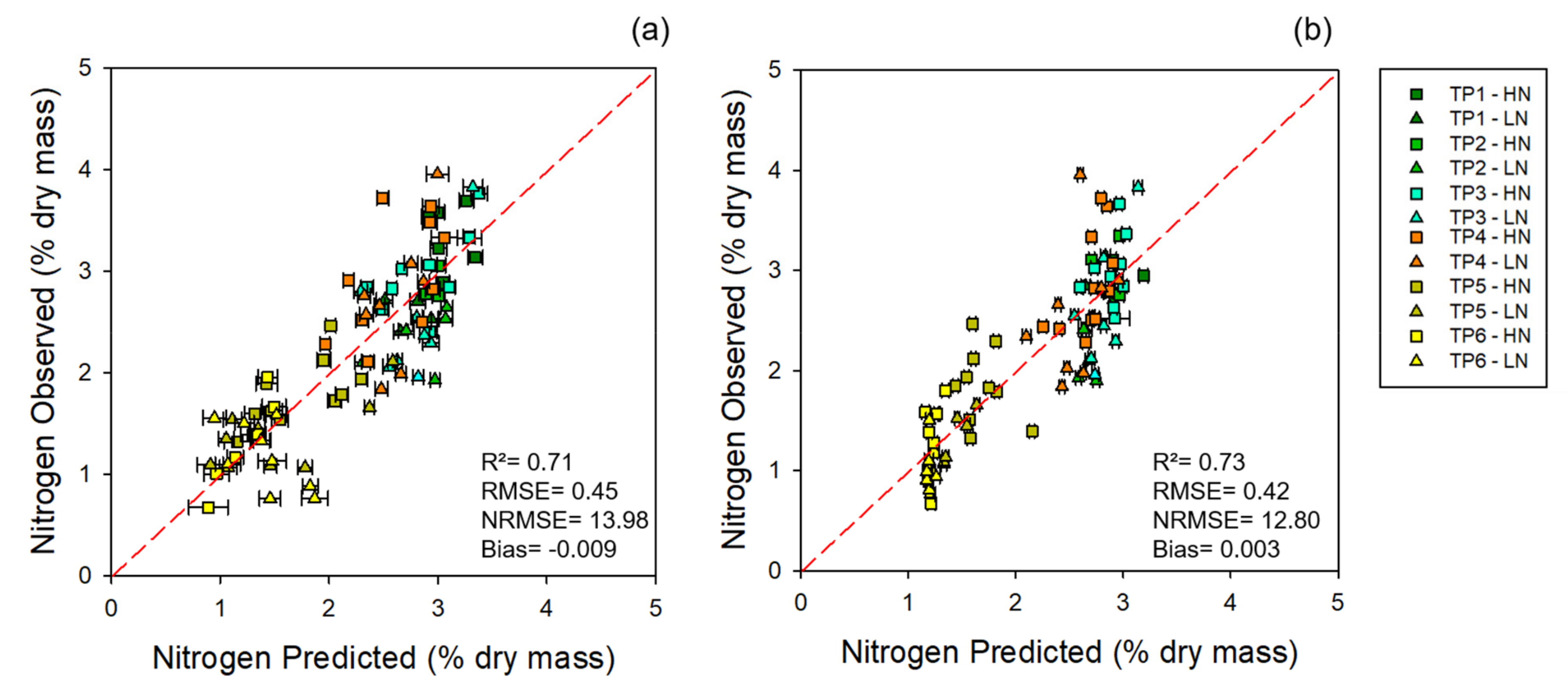
| Data Level | LV | R2 | RMSE | NRMSE (%) | Bias | ||||||||
|---|---|---|---|---|---|---|---|---|---|---|---|---|---|
| C | CV | EV | C | CV | EV | C | CV | EV | C | CV | EV | ||
| Leaf | 5 | 0.90 ± 0.00 | 0.84 ± 0.02 | 0.71 | 0.24 ± 0.01 | 0.31 ± 0.02 | 0.45 | 8 | 10 | 14 | 4.10 × 10⁻¹⁸ ± 0.02 | −0.0002 ± 0.05 | −0.009 |
| Canopy | 6 | 0.87 ± 0.01 | 0.85 ± 0.02 | 0.73 | 0.27 ± 0.01 | 0.3 ± 0.02 | 0.42 | 9 | 9 | 13 | 4.89 × 10⁻¹⁸ ± 0.02 | −0.0015 ± 0.04 | 0.003 |
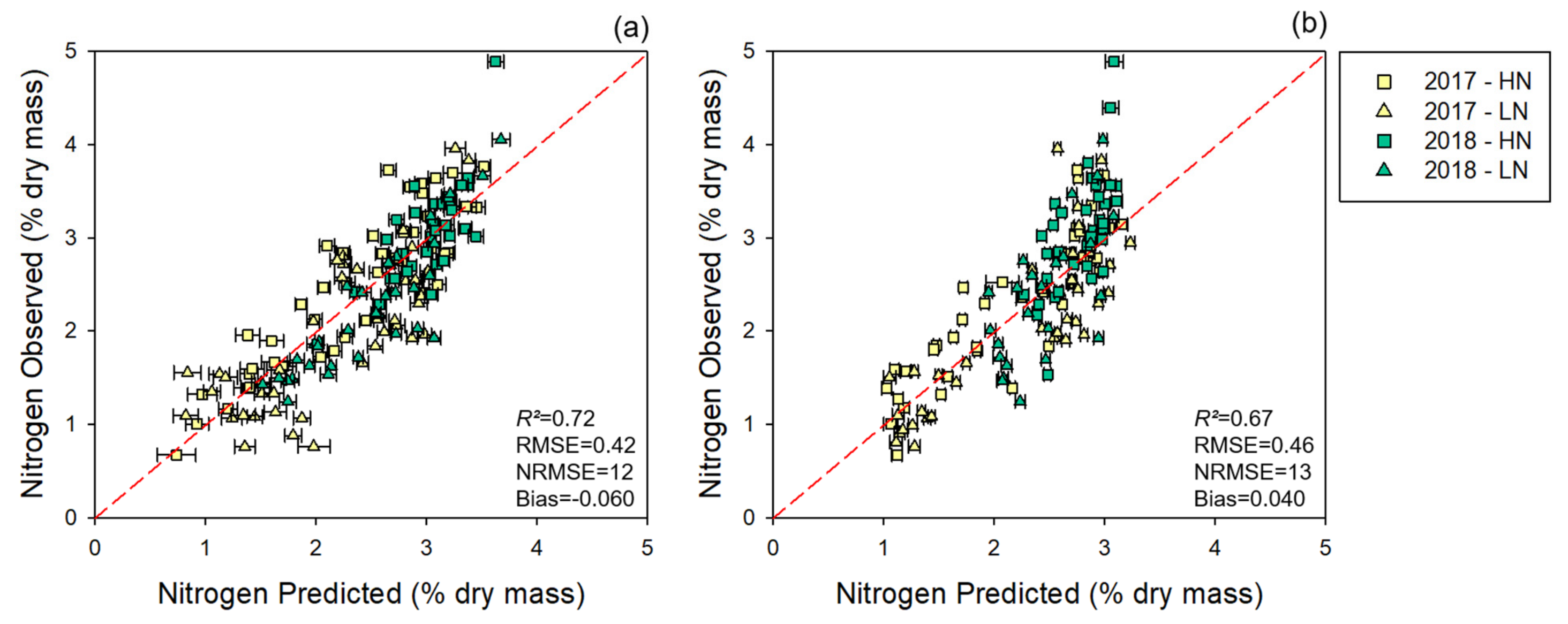
| Data Level | LV | R2 | RMSE | NRMSE (%) | Bias | ||||||||
|---|---|---|---|---|---|---|---|---|---|---|---|---|---|
| C | CV | EV | C | CV | EV | C | CV | EV | C | CV | EV | ||
| Leaf | 6 | 0.89 ± 0.01 | 0.84 ± 0.01 | 0.72 | 0.01 ± 0.01 | 0.32 ± 0.01 | 0.42 | 7 | 10 | 12 | −1.2 × 10⁻¹⁷ ± 0.00 | −0.0043 | −0.06 |
| Canopy | 5 | 0.87 ± 0.01 | 0.84 ± 0.02 | 0.67 | 0.26 ± 0.01 | 0.29 ± 0.02 | 0.46 | 9 | 10 | 13 | 5.98 × 10¹⁸ ± 0.00 | −0.0016 | 0.04 |
Publisher’s Note: MDPI stays neutral with regard to jurisdictional claims in published maps and institutional affiliations. |
© 2021 by the authors. Licensee MDPI, Basel, Switzerland. This article is an open access article distributed under the terms and conditions of the Creative Commons Attribution (CC BY) license (https://creativecommons.org/licenses/by/4.0/).
Share and Cite
Peron-Danaher, R.; Russell, B.; Cotrozzi, L.; Mohammadi, M.; Couture, J.J. Incorporating Multi-Scale, Spectrally Detected Nitrogen Concentrations into Assessing Nitrogen Use Efficiency for Winter Wheat Breeding Populations. Remote Sens. 2021, 13, 3991. https://0-doi-org.brum.beds.ac.uk/10.3390/rs13193991
Peron-Danaher R, Russell B, Cotrozzi L, Mohammadi M, Couture JJ. Incorporating Multi-Scale, Spectrally Detected Nitrogen Concentrations into Assessing Nitrogen Use Efficiency for Winter Wheat Breeding Populations. Remote Sensing. 2021; 13(19):3991. https://0-doi-org.brum.beds.ac.uk/10.3390/rs13193991
Chicago/Turabian StylePeron-Danaher, Raquel, Blake Russell, Lorenzo Cotrozzi, Mohsen Mohammadi, and John J. Couture. 2021. "Incorporating Multi-Scale, Spectrally Detected Nitrogen Concentrations into Assessing Nitrogen Use Efficiency for Winter Wheat Breeding Populations" Remote Sensing 13, no. 19: 3991. https://0-doi-org.brum.beds.ac.uk/10.3390/rs13193991