Communication

Sentinel-1 and RADARSAT Constellation Mission InSAR Assessment of Slope Movements in the Southern Interior of British Columbia, Canada

1
Canada Centre for Mapping and Earth Observation (CCMEO), Natural Resources Canada, Ottawa, ON K1S 5K2, Canada
2
Geological Survey of Canada (GSC), Natural Resources Canada, Ottawa, ON K1A 0E8, Canada
*
Author to whom correspondence should be addressed.
Remote Sens. 2021, 13(19), 3999; https://0-doi-org.brum.beds.ac.uk/10.3390/rs13193999
Submission received: 31 August 2021 / Revised: 28 September 2021 / Accepted: 30 September 2021 / Published: 6 October 2021
(This article belongs to the Special Issue RADARSAT Constellation Mission (RCM))

Abstract

:
Landslides are the most common natural hazard in British Columbia. The province has recorded the largest number of historical landslide fatalities in Canada, and damage to infrastructure comes at a great cost. In order to understand the potential impacts of landslides, radar remote sensing has become a cost-effective method for detecting downslope movements. This study investigates downslope movements in the Southern Interior of British Columbia, Canada, with Sentinel-1 and RADARSAT Constellation Mission (RCM) interferometric synthetic aperture radar (InSAR) data. The 2-dimensional time-series analysis with Sentinel-1 ascending and descending InSAR pairs from October 2017 to June 2021 observed distinct earthflow movements of up to ~15 cm/year in the east–west direction. The Grinder Creek, Red Mountain, Yalakom River, and Retaskit Creek earthflows previously documented are still active, with east–west movements of ~30 cm over the past four years. New RCM data acquired from June 2020 to September 2020 with a 4-day revisit capability were compared to 12-day Sentinel-1 InSAR pairs. The 4-day RCM InSAR pairs at higher spatial resolution showed better performance by detecting relatively small-sized slope movements within a few hundred meters, which were not clearly observed by Sentinel-1. The temporal variabilities observed from the RCM InSAR showed great potential for observing detailed slope movements within a narrower time window.

Graphical Abstract

1. Introduction

Historically, landslides have had catastrophic impacts, in Canada, in terms of loss of life and damage to infrastructure. Since 1771, there have been at least 786 fatalities due to landslides [1]. Damage to infrastructure has cost millions of Canadian dollars annually in repair and mitigation [2,3]. Furthermore, Porter et al. (2019) estimated that, in the Western Canadian Basin alone, costs related to landslide damage or prevention exceed CAD 281–450 million per year [4]. In British Columbia (BC)’s mountainous regions, landslides pose an ever-present risk [1,5,6]. Since 1880, there have been at least 356 landslide fatalities in BC caused by a variety of landslide types, such as rockfalls, rockslides, rock avalanches, debris flows, etc. [1]. Recently, in November 2020, a massive landslide occurred along the steep mountainous slopes over Elliot Creek in BC, which triggered a tsunami in a glacial lake and a subsequent outburst flood carrying ~7.7 million cubic meters of mud and rock debris into Bute Inlet, reshaping the coastal landscape [7]. In January 2021, mud and rocks slid into Harrison Lake from a steep slope of Mount Breakenridge in BC over two days. A bathymetric survey of Harrison Lake reported that ~4 million cubic meters of landslide debris were deposited on the lake floor, which implies the potential for tsunamigenic landslides [8]. Furthermore, accelerated glacier melting and retreat can increase landslide activity in high mountainous areas, as observed in BC [7,9].
With limited physical access to remote areas and infeasibility of ground monitoring of potential landslide events, interferometric synthetic aperture radar (InSAR) has become a promising tool for observing slope movements at a mm–cm scale from a regional perspective and in a timely manner. Since the 1990s, InSAR has been extensively used for monitoring landslides by applying the differential InSAR (DInSAR) [10,11,12,13,14], permanent scatter InSAR (PSI) [15,16,17,18,19,20,21], or InSAR coherence-based [22,23] techniques. However, it is very challenging to obtain a sufficient coherence to generate interferograms between InSAR acquisitions before and after landslide events, particularly in the case of rapid and large gradient deformation [24]. Other challenges are atmospheric noise, vegetation, and seasonal effects, such as rainfall and snow [25]. Therefore, time-series analyses are necessary to mitigate the contributions from noise and non-deformation signals. In this respect, the freely available global coverage acquisitions of Sentinel-1 have provided a great advantage for time-series landslide monitoring [25,26,27]. In addition, a trio of RADARSAT Constellation Mission (RCM) satellites with a 4-day revisit capability have great potential for monitoring slope movement increments more precisely than with 12-day Sentinel-1 and 24-day RADARSAT-2 acquisitions [28].
At Natural Resources Canada (NRCan), the Canadian Centre for Remote Sensing (CCRS) and the Geological Survey of Canada (GSC)’s Public Safety Geoscience Program (PSGP) have collaborated to test Sentinel-1 and newly launched RCM satellites for landslide monitoring. The PSGP has the mandate to support risk reduction of natural hazards by providing baseline geoscience information to stakeholders and decision-makers. Consequently, the objectives of this study are to (1) identify active areas showing downslope movements with InSAR, (2) assess the amount of slope movements, and (3) evaluate the performance of Sentinel-1 and RCM sensors.

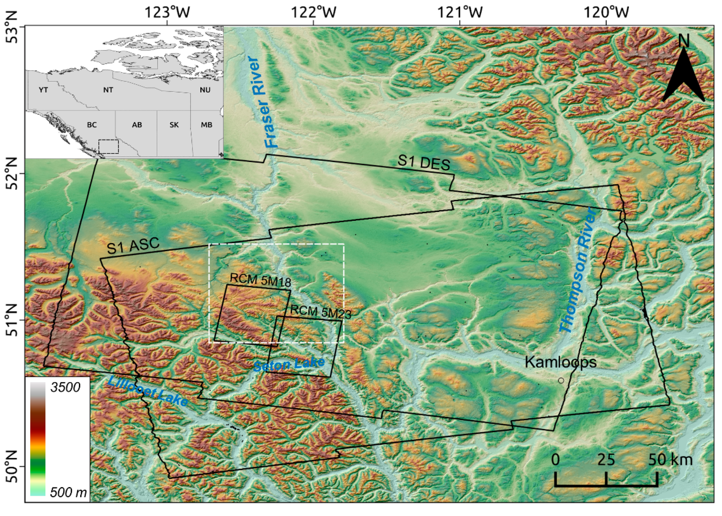
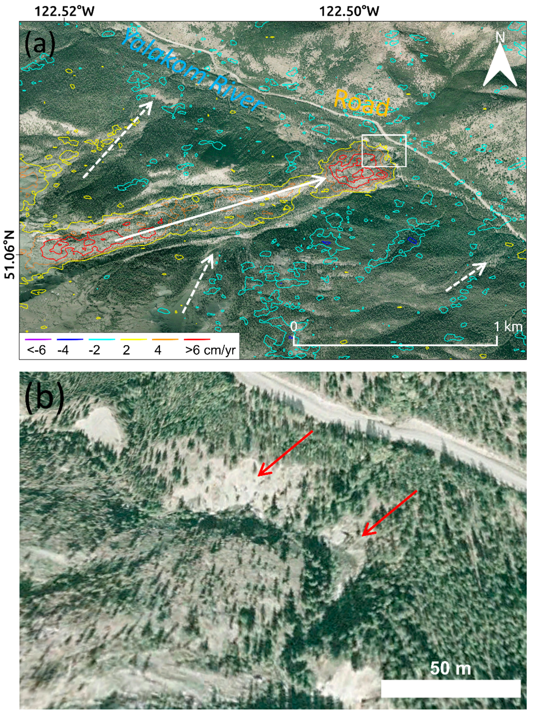
2. Geological Setting

The study area of roughly 50,000 km2 within British Columbia’s Southern Interior (Figure 1) belongs to the northwest–southeast trending morphogeological belts of the Coast and Intermontane belts [29]. The Coast belt is mainly formed of granitic plutons ranging from the Jurassic to Cenozoic in age. Other rock types are volcanic and sedimentary in origin, dating from the late Proterozoic, to the Paleozoic and Holocene. Some were highly metamorphosed from mid-Cretaceous to early Ceneozoic time. The Intermontane rocks consist of a variety of volcanic, sedimentary, and granitic rocks from the Devonian to the Jurassic, to early Cenozoic [29].
The Fraser Glaciation in southern British Columbia began in Late-Wisconsinan time, about 29,000 years BP, culminated about 14,000 years BP, with deglaciation almost complete around 11,500 years BP [30]. The highest elevation in the study area is roughly 2600 m and the lowest is about 350 m (Figure 1).
The study area encompasses at least three biogeoclimatic zones: Montane spruce, Engelman Spruce–Subalpine Fir, Interior Douglas Fir [31]. The Montane Spruce zone is a narrow mid-elevation band (300–400 m) of vegetation. However, it can be found at high-elevation plateaus between 1100–1650 m. It reflects a cool dry climate with average temperatures above 10 ℃ for 2–4 months a year and below 0 ℃ for 5 months a year. Precipitation varies between 300 and 900 mm per year. The Engelman Spruce–Subalpine Fir zone occupies the highest elevations in British Columbia. It reflects cold long snowy winters and short cool summers. Average annual temperatures range from −2 to 2 ℃, and average annual precipitation is highly variable from 400–500 mm in drier areas up to 2200 mm in wetter areas. The Interior Douglas Fir zone occupies low–mid elevations where summers are short, warm and dry with mild winters. There is often a shortage of moisture during the growing season. Average annual temperatures vary from 1.6 to 9.5 ℃ and annual precipitation ranges from 300 to 750 mm, but can exceed 1000 mm in wetter areas [31].
An historical photogrammetric survey of earthflows within the study area by Bovis and Jones (1992) reported that these were “glacier-like masses of soil and rock, typically 0.5–1 km wide and 2–6 km long, which move at velocities of 0.5 m/year” (p. 1746) [32]. The study revealed, through dendrochronology and tephrochronology, that many responded to the same hydroclimatic changes over time. Reactivation of the earthflows reflected cooler and wetter conditions, which produced an increase in groundwater recharge and pore water pressure at different times during the Holocene [32]. Some of these earthflows are further discussed in the Results (Section 4) and Discussion (Section 5).

3. Materials and Methods

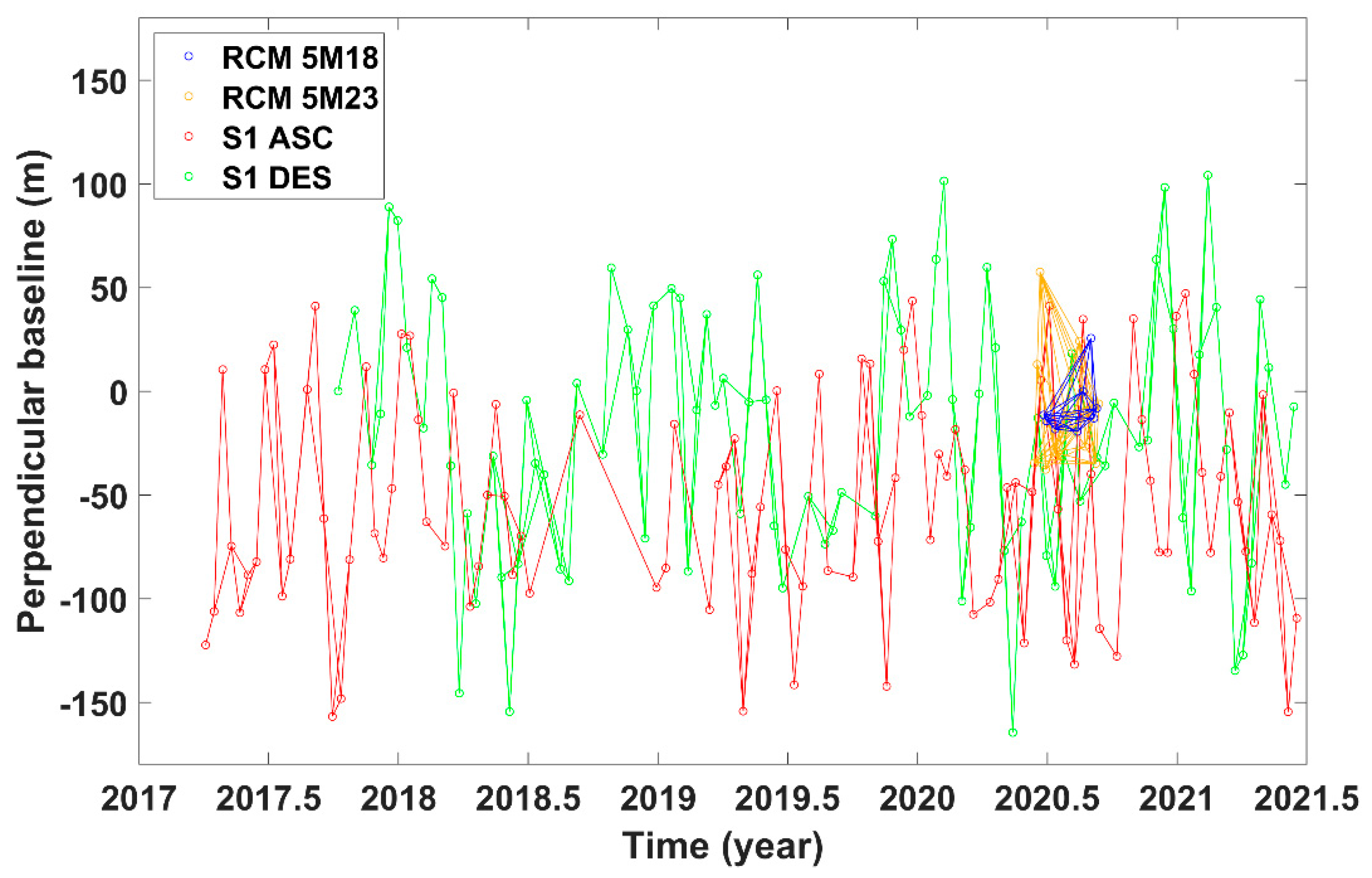
3.1. Sentinel-1 and RCM Data

A total of 102 ascending (path: 64, frame: 163, April 2017–June 2021) and 91 descending (path: 13, frame: 421, October 2017–June 2021) Sentinel-1 Terrain Observation with Progressive Scan (TOPS) SAR data of VV polarization were processed (Table 1 and Figure 2). The Sentinel-1 TOPS SAR single look complex (SLC) data were acquired at a spatial resolution of 2.3 m by 13.9 m in range and azimuth, respectively, at incidence angles of ~30–45°. The Sentinel-1 TOPS SAR interferometric wide (IW) mode data, with a ~250 km wide swath, consist of 27 and 28 burst images for ascending and descending, respectively. They were acquired with a 12-day repeat cycle (cf. 6-day revisit available with the Sentinel-1A and Sentinel-1B constellation) [33]. A total of 8 descending RCM 5M18 mode SLC images and 14 descending RCM 5M23 mode SLC images of HH polarization acquired from June 2020 to September 2020 were processed. The RCM SLC data were acquired at a spatial resolution of 2.7 m by 2.5 m in range and azimuth at incidence angles of 47° (5M18 mode) and 53° (5M23 mode), respectively. The 5 m resolution RCM data provide a ~30 km swath and a repeat cycle up to 4-days.

3.2. InSAR Processing

InSAR measures the phase difference in line-of-sight (LOS) between two SAR acquisitions. The phase difference modulated in 2π can be unwrapped into the displacements at a cm-scale wavelength. The InSAR processing was performed with an automated InSAR processor based on the GAMMA software of the NRCan’s Earth Observation Data Management System (EODMS) [34,35]. Based on small perpendicular and temporal baselines, multi-master InSAR pairs were selected and precisely co-registered for each pair. The interferograms were generated by multilooking, with a window of 4 by 1 pixels in range and azimuth (i.e., corresponding to 9.2 m by 13.9 m) for Sentinel-1 and a window of 2 by 4 pixels in range and azimuth (i.e., corresponding to 5.4 m by 10 m) for RCM. Note that a window of 2 by 1 pixels in range and azimuth (i.e., corresponding to 4.6 m by 13.9 m) was applied for Sentinel-1 processing for the comparison with RCM acquisitions from June 2020 to September 2020 to minimize the difference of the range resolution. The topographic phase was removed with the 30 m resolution Canadian Digital Elevation Model (CDEM). The multilooked DInSAR interferograms were filtered by the Goldstein adaptive filter [36] and unwrapped by the minimum cost flow (MCF) algorithm [37]. One-dimensional (1D, LOS) and two-dimensional (2D, east–west and vertical) time-series analyses were performed by applying the multidimensional small baseline subset (MSBAS) technique [38,39,40]. The 2D east–west and vertical movements were reconstructed by using the following Equation (1),
( A ^ λ L ) ( V E V V ) = ( Φ ^ 0 ) ,   ( V E V V ) = ( A ^ λ L ) + ( Φ ^ 0 )
where A ^ = { cos φ sin θ A ,   cos θ A } , A is a matrix constructed from the time intervals of ascending and descending SAR acquisitions, φ is the azimuth angle, θ is the incidence angle, and λ and L are a regularization parameter and the Tikhonov regularization matrix, respectively [38,39,40]. V E and V V are vectors of the unknown east–west and vertical velocities (cf. the north–south component, V N , is neglected as V N   V E ,   V ), Φ ^ is a vector of the observed DInSAR deformation values, and A ^ + is the pseudo-inverse of matrix A ^ [38,39,40].

4. Results

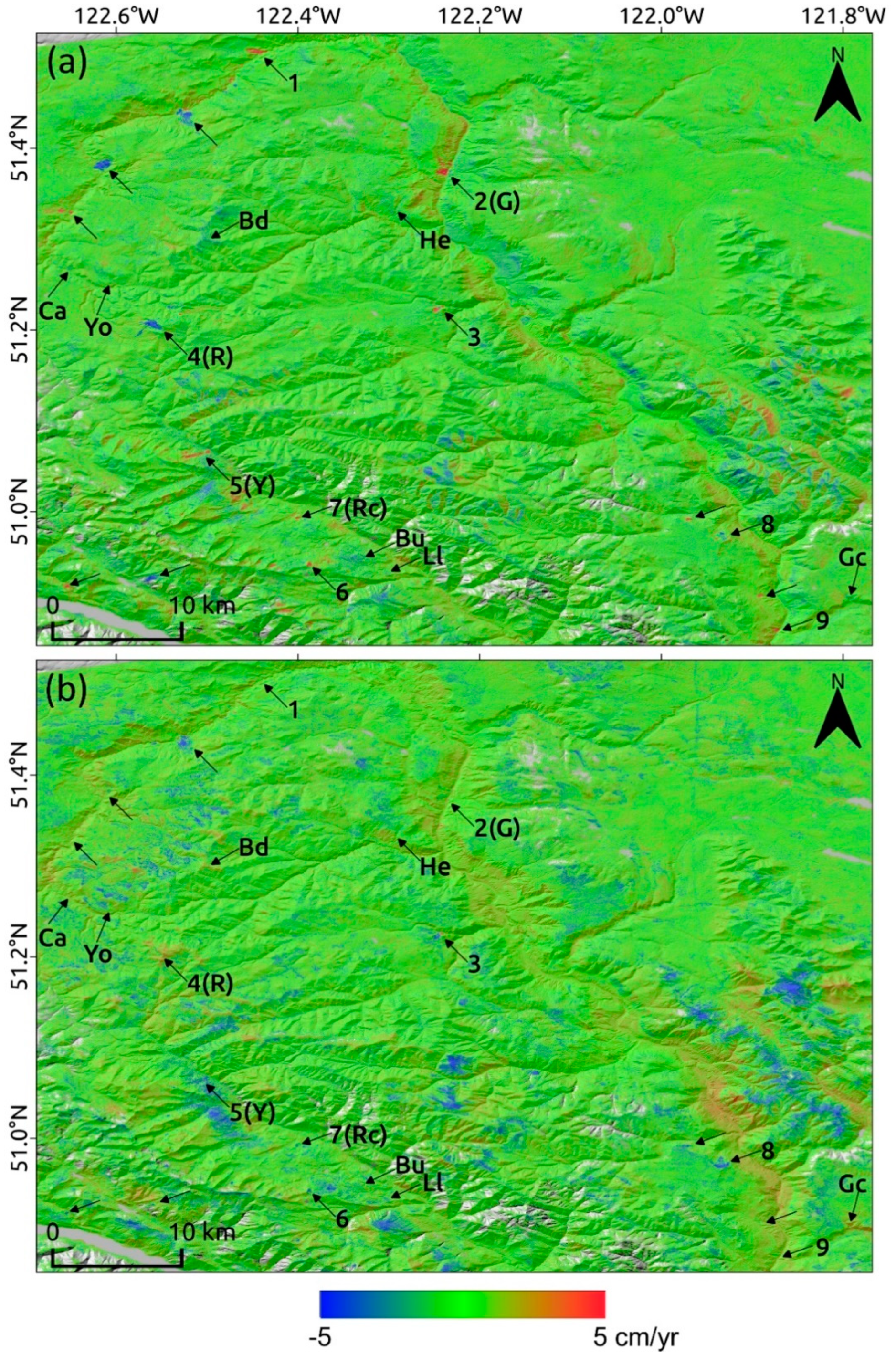
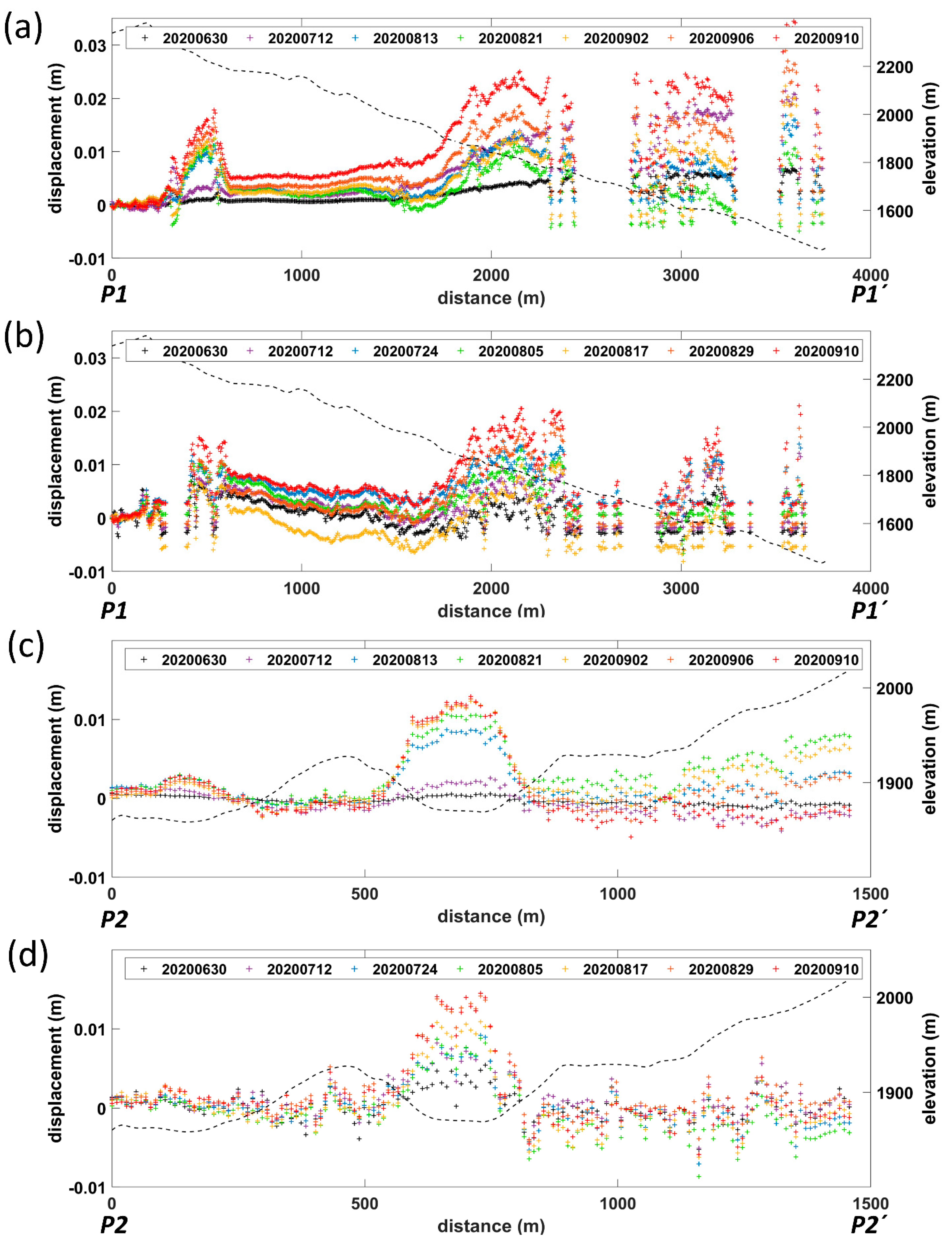
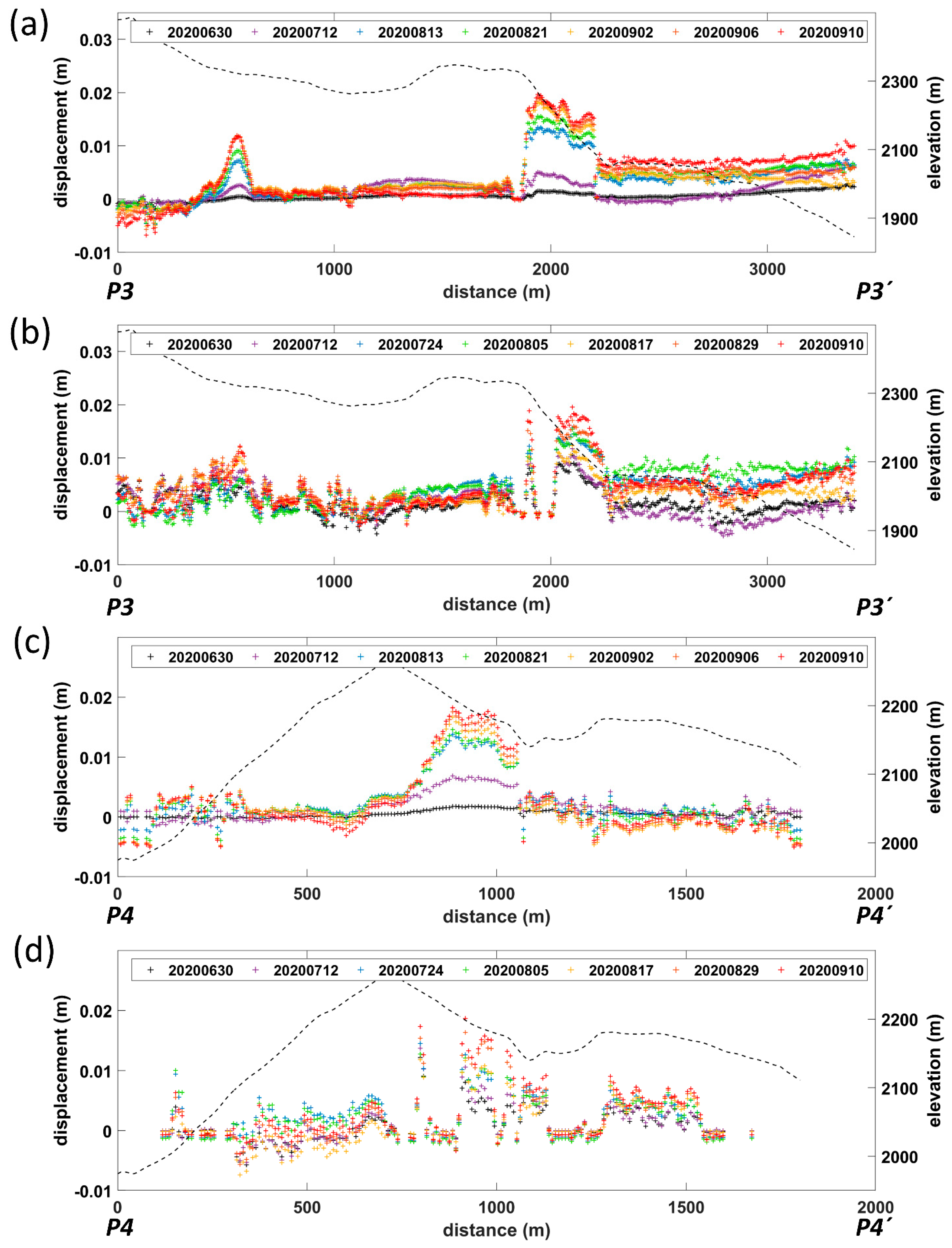
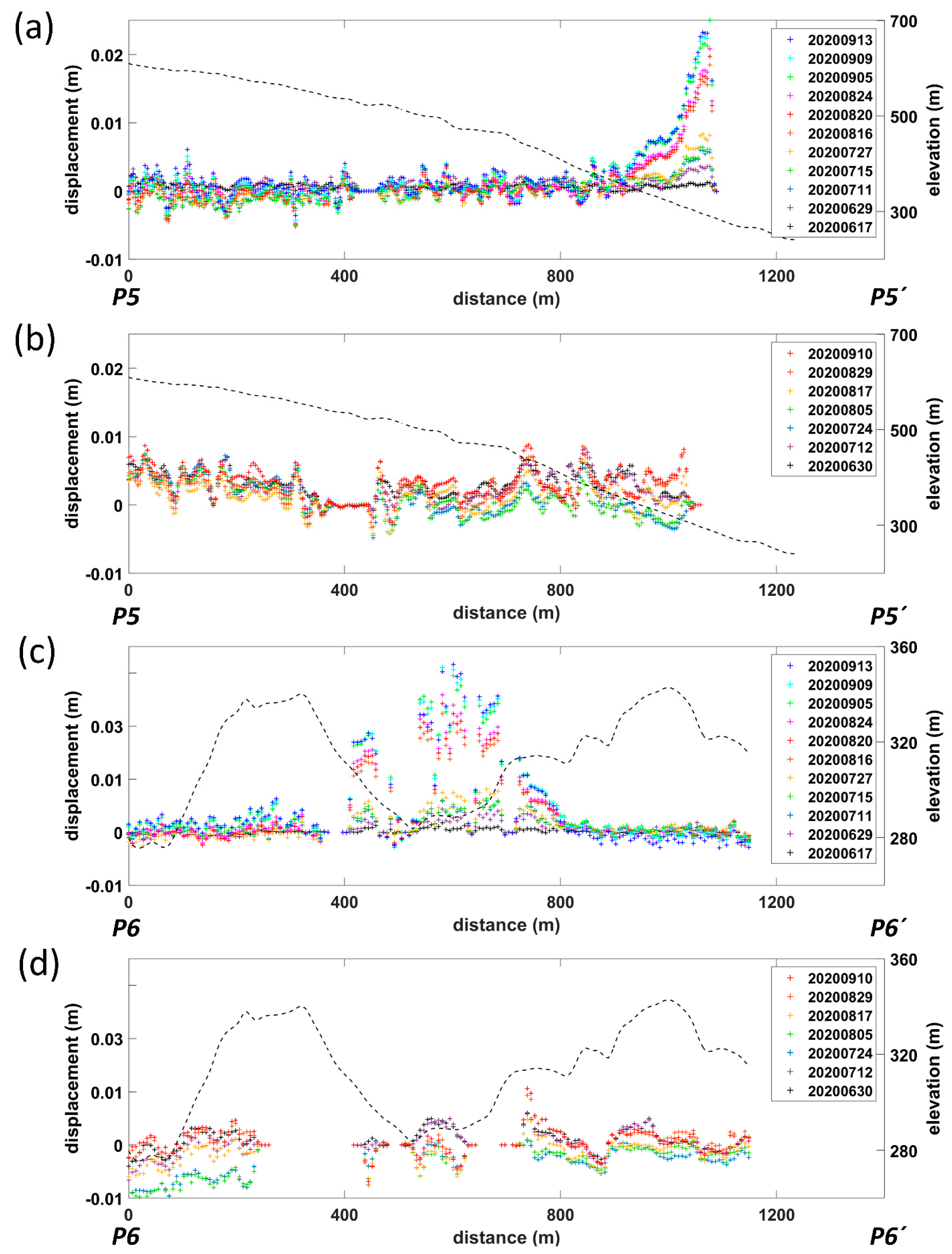
4.1. Sentinel-1 2D MSBAS Time-Series Analysis

Figure 3 shows the linear deformation rate maps of east–west and vertical movements, which were reconstructed from Sentinel-1 ascending and descending time-series InSAR pairs. Slope movements are distinctly characterized by east–west components, which range from ~–12 cm/year to ~15 cm/year (i.e., positive values mean eastward movements). The east–west movements correspond to the downward directions of slopes and are dominantly observed from shallow to moderate slopes in valleys, including river channels. Vertical movements are relatively small and not as distinct as the east–west movements, as shown in Sites 1, 2, and 9 (Figure 3b). Vertical movements are rarely observed from slopes shallower than ~10°. Most of the significant vertical movements are observed around mountain tops above ~1700 m, which indicate downward movements of ~–10 cm/year.
Figure 4, Figure 5 and Figure 6 represent examples of earthflows observed on Google Earth imagery with their east–west movements and time-series displacement plots measured from the Sentinel-1 2D MSBAS analysis. Cumulative east–west (blue) and vertical (purple) movements between October 2017 and June 2021 were extracted from 5-by-5 pixels for each site. The average standard deviations range from 0.7 cm (Site 1) to 3.3 cm (Site 5) for east–west movements and from 1.1 (Site 9) cm to 2.3 cm (Sites 4 and 7) for vertical movements, respectively. In particular, Grinder Creek (G = Site 2; Figure 4b), Red Mountain (R = Site 4; Figure 5a), Yalakom River (Y = Site 5; Figure 5b) [32] and Retaskit Creek (Rc = Site 7; Figure 6a) [41], among the documented earthflows, are still active, with east–west movements of up to ~30 cm over the past four years. No significant east–west and vertical movements are observed from Heginbottom Creek (He), Black Dome (Bd), Canyon (Ca), Yodel (Yo), Burkholder Creek (Bu), Lac La Mer (Ll), and Gillon Creek (Gc) earthflows (Figure 3). Additional slope movements other than the earthflows documented by [32,41] are observed on the east–west movement map (Figure 3a), which include Sites 1, 3, 6, 8, and 9 showing east–west movements of up to ~50 cm over four years (Figure 4, Figure 5 and Figure 6).

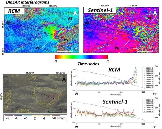
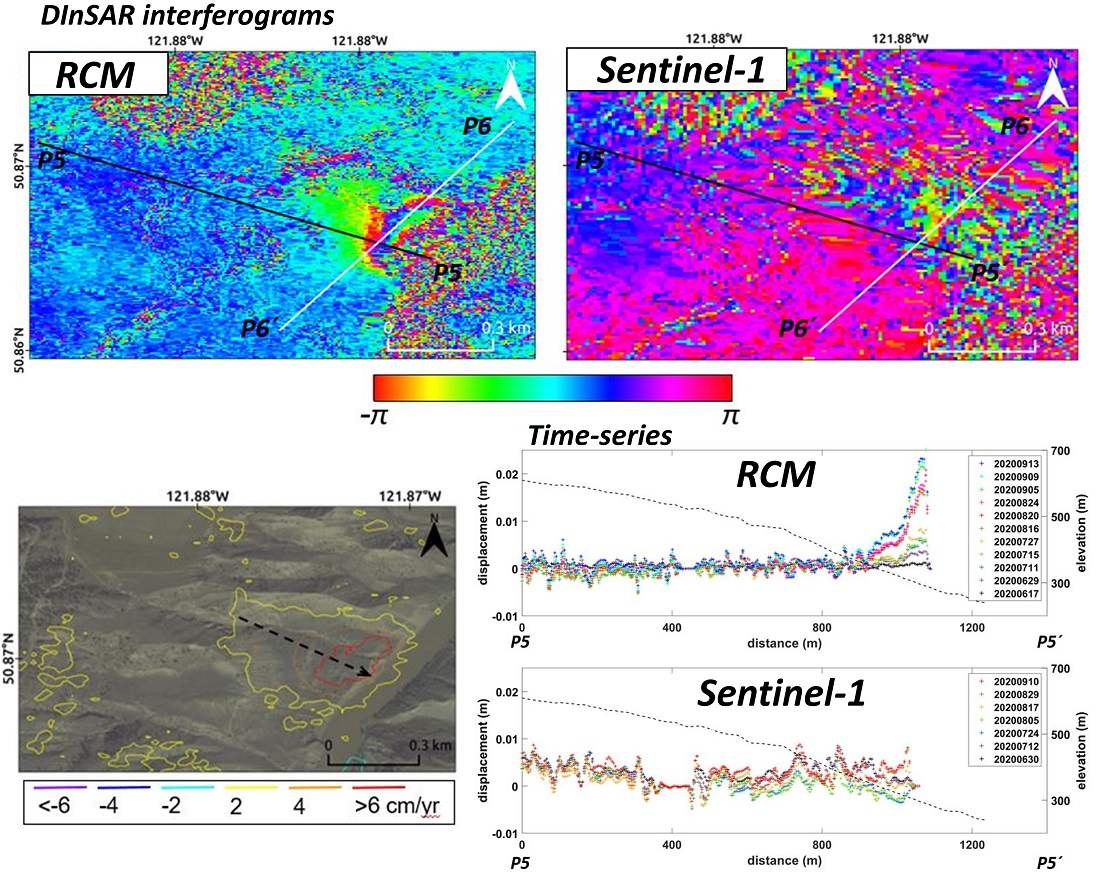
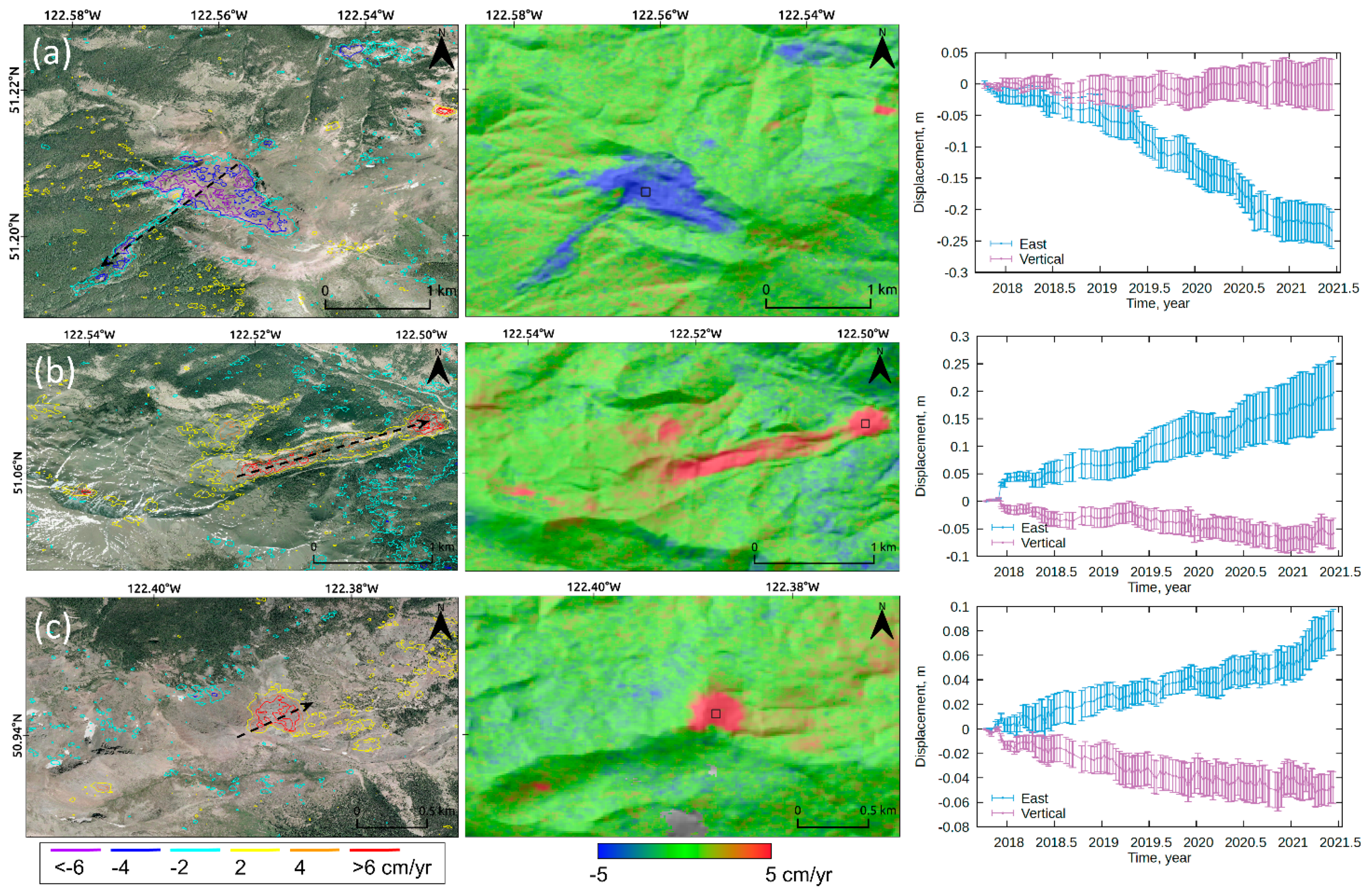
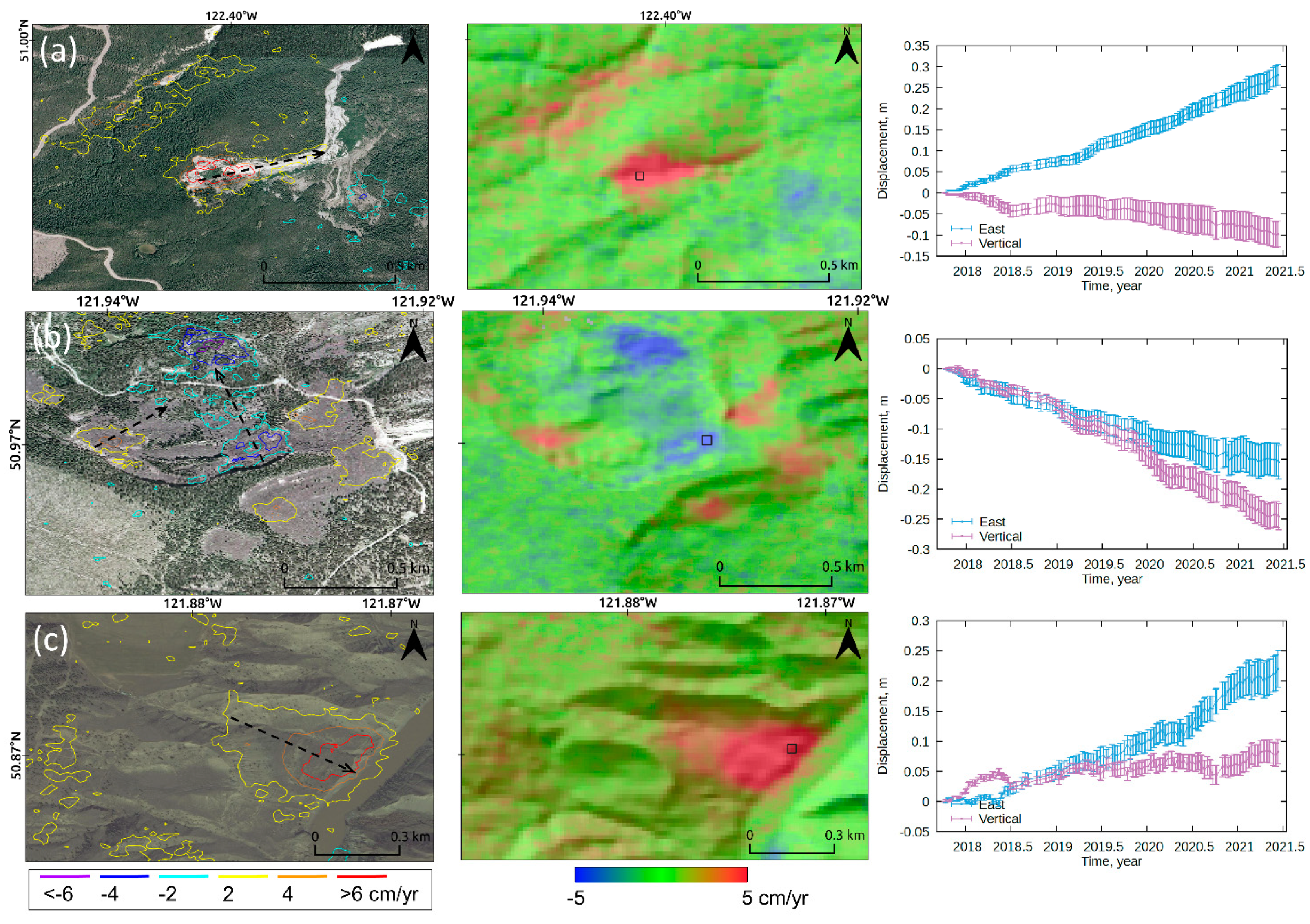
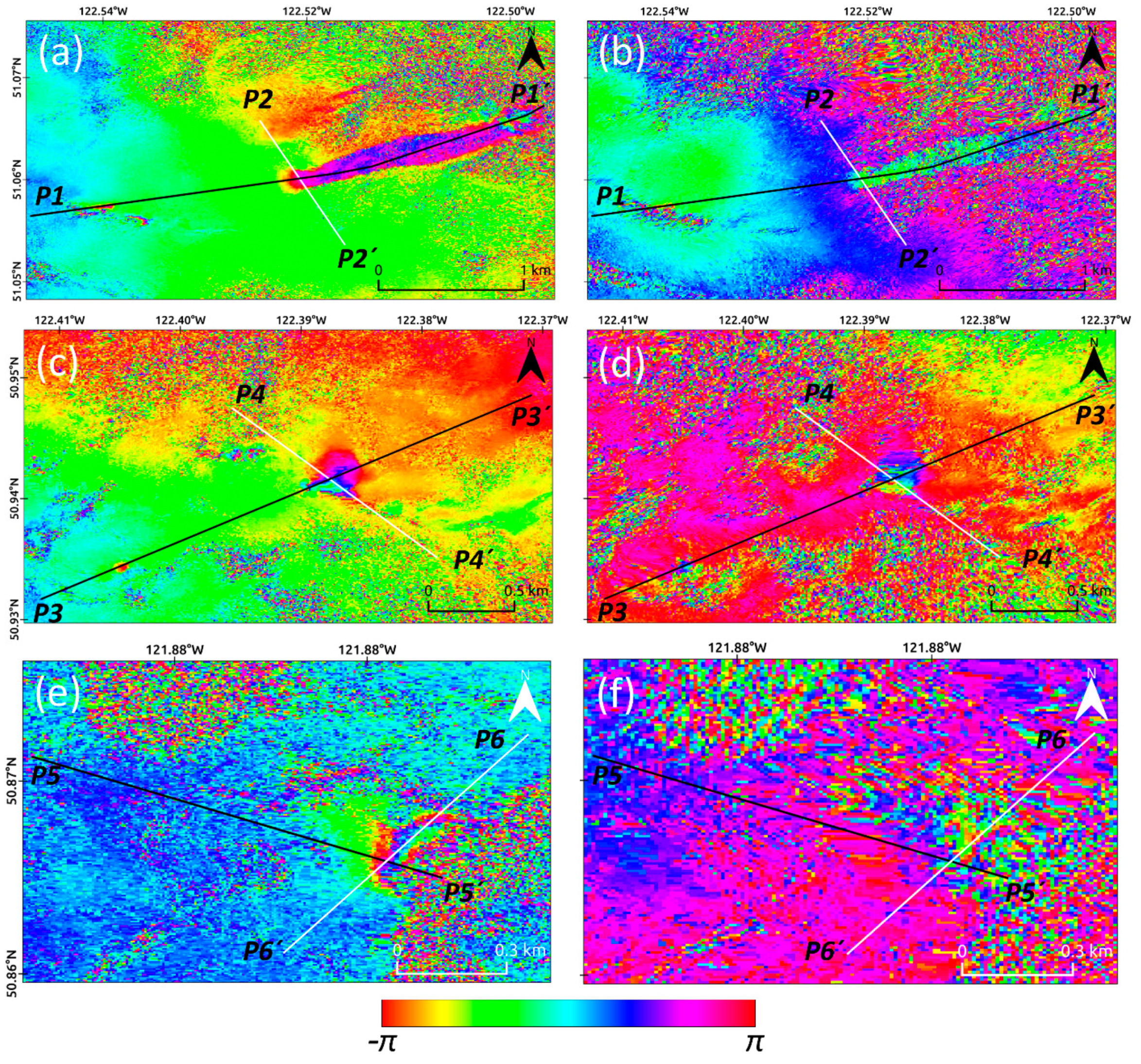
4.2. Comparison between Sentinel-1 and RCM

Figure 7 shows the RCM interferograms of Sites 5, 6, and 9, compared to the Sentinel-1 interferograms. More detailed fringe patterns from small slope movements between tens of meters (e.g., fringes close to P1 and P1′ in Figure 7a and P3 in Figure 7c) and ~300 m in length are better captured by the RCM, which are not clearly differentiated from noise with Sentinel-1. In particular, the RCM captured a full DInSAR fringe from very small slope movements within ~300 m in length in Site 9 (Figure 7e). The time-series profile analysis from June 30 to September 10, 2020, shows a similar range of displacements in both Sentinel-1 and RCM (Figure 8, Figure 9 and Figure 10), but the RCM provided better spatial and temporal resolutions. In particular, significant movements are observed between mid-July and mid-August, based on the RCM results (e.g., 12 July–13 August in Figure 8 and Figure 9, 15 July–16 August in Figure 10). For slope movements within ~300 m in length in Site 9, the Sentinel-1 results (~1 cm) are significantly fewer than the RCM results (~2 cm) (Figure 10).

5. Discussion

The extensive Sentinel-1 TOPS SAR global coverage archives provide a great advantage for monitoring time-series slope movements from a regional perspective. East–west and vertical movements are reconstructed from ascending and descending LOS displacements. LOS measurements are insensitive to north–south movements due to the imaging geometry of near-polar orbiting sensors [38]. The observed slope movements in the area of interest are slow-moving earthflows and are better measurable in the east–west direction (<~15 cm/year). The east–west movement rates estimated from the Sentinel-1 DInSAR correspond to the lower range of the earthflow movement rates at ~0.1 to 5 m/year documented in [32]. Vertical movements are small, relative to east–west movements and rarely observed from shallow slopes. Earthflows at shallow slope gradients show little vertical movements, though they show significant east–west movements (see Sites 1, 2, 9 in Figure 3a,b). The significant vertical movements around the mountain tops are observed only during winter months (i.e., ~December–March), which are likely to be related to ice and/or snow dynamics at high elevations.
Overall, the LOS displacements estimated from Sentinel-1 and RCM show similar patterns and amounts, but more detailed spatial and temporal variabilities observed from the RCM are not achieved by Sentinel-1. This is because the azimuth resolution of Sentinel-1 (13.9 m) is much coarser than that of the RCM (2.5 m), while the range resolution of Sentinel-1 (2.3 m) is comparable to that of the RCM (2.7 m). Though the range spacing of Sentinel-1 is achieved close to that of the RCM during the processing, the details of slope movements, particularly from earthflows within ~300 m in length, can be lost due to the azimuth spacing of more than 5 times, possibly resulting in saturation or underestimation of displacement measurements. There are differences in polarization and incidence angles between the Sentinel-1 and RCM acquisitions, but these have little impact on displacement measurements, given the similarities in the pattern and amounts of displacements observed from large-sized slope movements over a few hundred meters (~1 km2).
Given the limited number of 4-day revisit RCM acquisitions and the slow movement rates of < ~15 cm/year in this region, it is not enough to assess the performance of 4-day repeat pass InSAR for monitoring slope movements. However, temporal variabilities observed from RCM 4-day (e.g., between 2 September 2020, 6 September 2020, and 10 September 2020, in Figure 8a) and 8-day (e.g., between 13 August 2020 and 21 August 2020, in Figure 8c) repeat passes show that the RCM 4-day repeat pass InSAR has great potential for observing more detailed slope movements with a better chance to obtain coherence, though the maximum detectable deformation gradient is limited to ~1.4 × 10³ (i.e., for a multilooked range pixel of ~10 m) [42].

Implications for Landslide Hazards and Risks

Both the Sentinel-1 and RCM DInSAR results demonstrate that certain types of landslides in the Southern Interior of British Columbia, especially earthflows, can be detected. Cumulative displacement amounts and displacement rates over a long period of time can be measured with time-series InSAR pairs. At a first glance, earthflows may not represent a high hazard, or risk, but slow and steady earthflows should be taken into consideration when building infrastructure, such as pipelines, roads, power lines, mines, etc. For example, Figure 11 shows close-up views of Google Earth imagery and the east–west movement rate of the largest earthflow (~2.4 km by 0.35 km) and other surrounding smaller earthflows at Yalakom River (i.e., Site 5 shown in Figure 3, Figure 5b and Figure 7a). The Sentinel-1 time-series results show that the average of the cumulative east–west movements is estimated at ~20 cm over four years for the largest earth flows at Yalakom River (see Figure 5b). This particular earthflow, triggered in weathered bedrock consisting of harzburgite, dunite, orthopyroxenite, and serpentinite mélange from the Shulaps Ultramafic complex [43], seems to have diverted the drainage of Yalakom River. This is slowly moving towards the road, causing riverbank erosion on the east side of the river channel. Hence, in this case, mitigation measures will have to be considered for future development projects.

6. Conclusions

Slow-moving earthflows in the southern interior of British Columbia were observed by the Sentinel-1 and RCM DInSAR analyses. The Sentinel-1 TOPS SAR provides both ascending and descending time-series data collected from 2017 with a broad coverage of ~250 km over this area. In addition to previously documented earthflows, numerous other slow-moving landslides were detected by the Sentinel-1 2D MSBAS analysis spanning four years. Earthflows are moving up to ~15 cm/year in the east–west direction, which correspond to the lower range of movement rates of documented earthflows. The Grinder Creek, Red Mountain, Yalakom River, and Retaskit Creek earthflows are very active, with east–west movements of ~30 cm over the past four years. The RCM provides much higher spatial resolution (i.e., 1 m spotlight, 3 m very-high-resolution and 5 m high-resolution modes) with a 4-day revisit capability, though the swath is limited to <~30 km with the high-resolution modes. Thus, it is recommended to initially observe slope movements at a regional scale by applying 2D time-series analysis with Sentinel-1 and then focus on slope movements of interest at high spatial and temporal resolution with the RCM. From a landslide hazard and risk perspective, slow-moving earthflows should be taken into consideration in development projects, as they can divert river drainage, which can, in turn, cause erosion of riverbanks and can affect infrastructure, as observed at Yalakom River.

Supplementary Materials

The geotiff format files of Figure 3 (Sentinel-1 linear deformation rate maps of east-west and vertical movements) and Figure 7 (RCM and Sentinel-1 DInSAR interferogram maps) are available at Mendeley Data (doi:10.17632/jtbw57ftyv.1).

Author Contributions

Conceptualization, B.-H.C., A.B.-S. and S.S.; methodology, B.-H.C. and S.S.; software, B.-H.C., S.S. and J.D.; validation, B.-H.C., A.B.-S. and S.S.; formal analysis, B.-H.C., A.B.-S., S.S. and J.D.; investigation, B.-H.C., A.B.-S., S.S. and J.D.; resources, A.B.-S. and S.S.; data curation, B.-H.C. and S.S.; writing—original draft preparation, B.-H.C.; writing—review and editing, B.-H.C., A.B.-S., S.S. and J.D.; visualization, B.-H.C.; supervision, A.B.-S. and S.S.; project administration, A.B.-S.; funding acquisition, A.B.-S. All authors have read and agreed to the published version of the manuscript.

Funding

This work was funded by Natural Resources Canada’s Office of Energy Research and Development (GSC-19-103) and the Public Safety Geoscience Program within the Geological Survey of Canada.

Data Availability Statement

The Sentinel-1 archives from the Alaska Satellite Facility (ASF) are available at https://search.asf.alaska.edu (accessed on 31 August 2021). The RCM and CDEM data are available at https://www.eodms-sgdot.nrcan-rncan.gc.ca (accessed on 31 August 2021).

Acknowledgments

The Sentinel-1 data were provided by the European Space Agency (ESA) and the RCM data were provided by the Canadian Space Agency (CSA). P. Friele of Cordilleran Geoscience provided suggestions for landslide monitoring sites. D. Huntley from GSC and two anonymous reviewers provided valuable comments that helped improve this manuscript. This is GSC contribution 20210206.

Conflicts of Interest

The authors declare no conflict of interest.

References

  1. Blais-Stevens, A. Historical landslides that have resulted in fatalities in Canada (1771–2019); Geological Survey of Canada, Open File 8392; Natural Resources Canada: Ottawa, ON, Canada, 2020. [Google Scholar]
  2. Hungr, O. Landslide Hazards in BC-Achieving Balance in Risk Assessment. Innovation 2004, 2004, 12–15. [Google Scholar]
  3. Guthrie, R. Socio-economic Significance-Canadian Technical Guidelines and Best Practices related to Landslides: A national initiative for loss reduction. Geol. Surv. Can. 2013, 7311, 315–322. [Google Scholar]
  4. Porter, M.; Van Hove, J.; Barlow, P.; Froese, C.; Bunce, C. The estimated economic impacts of prairie landslides in western Canada. In Proceedings of the 72nd Canadian Geotechnical Conference, St. John’s, NL, Canada, 29 September–2 October 2019. [Google Scholar]
  5. Blais-Stevens, A.; Septer, D. Historical Accounts of Landslides and Flooding Events along the Sea to Sky Corridor, British Columbia, from 1855–2007; Geological Survey of Canada, Open File 5741; Natural Resources Canada: Ottawa, ON, Canada, 2008. [Google Scholar]
  6. Strouth, A.; McDougall, S. Historical Landslide Fatalities in British Columbia, Canada: Trends and Implications for Risk Management. Front. Earth Sci. 2021, 9, 1–8. [Google Scholar] [CrossRef]
  7. Geertsema, M.; Menounos, B.; Shugar, D.; Millard, T.; Ward, B.; Ekstrom, G.; Clague, J.; Lynett, P.; Friele, P.; Schaeffer, A.; et al. A landslide-generated tsunami and outburst flood at Elliot Creek, coastal British Columbia. In Proceedings of the EGU General Assembly 2021, Vienna, Austria, 19–30 April 2021. [Google Scholar]
  8. Hughes, K.E.; Geertsema, M.; Kwoll, E.; Koppes, M.N.; Roberts, N.J.; Clague, J.J.; Rohland, S. Previously undiscovered landslide deposits in Harrison Lake, British Columbia, Canada. Landslides 2021, 18, 529–538. [Google Scholar] [CrossRef]
  9. Liu, J.; Wu, Y.; Gao, X. Increase in occurrence of large glacier-related landslides in the high mountains of Asia. Sci. Rep. 2021, 11, 1–12. [Google Scholar]
  10. Fruneau, B.; Achache, J.; Delacourt, C. Observation and modelling of the Saint-Étienne-de-Tinée landslide using SAR interferometry. Tectonophysics 1996, 265, 181–190. [Google Scholar] [CrossRef]
  11. Rott, H.; Scheuchl, B.; Siegel, A.; Grasemann, B. Monitoring very slow slope movements by means of SAR interferometry: A case study from a mass waste above a reservoir in the Ötztal Alps, Austria. Geophys. Res. Lett. 1999, 26, 1629–1632. [Google Scholar] [CrossRef]
  12. Singhroy, V.; Molch, K. Characterizing and monitoring rockslides from SAR techniques. Adv. Sp. Res. 2004, 33, 290–295. [Google Scholar] [CrossRef]
  13. Strozzi, T.; Farina, P.; Corsini, A.; Ambrosi, C.; Thüring, M.; Zilger, J.; Wiesmann, A.; Wegmüller, U.; Werner, C. Survey and monitoring of landslide displacements by means of L-band satellite SAR interferometry. Landslides 2005, 2, 193–201. [Google Scholar] [CrossRef]
  14. Handwerger, A.L.; Roering, J.J.; Schmidt, D.A. Controls on the seasonal deformation of slow-moving landslides. Earth Planet. Sci. Lett. 2013, 377–378, 239–247. [Google Scholar] [CrossRef]
  15. Ferretti, A.; Prati, C.; Rocca, F. Permanent scatterers in SAR interferometry. IEEE Trans. Geosci. Remote Sens. 2001, 39, 8–20. [Google Scholar] [CrossRef]
  16. Colesanti, C.; Ferretti, A.; Prati, C.; Rocca, F. Monitoring landslides and tectonic motions with the Permanent Scatterers Technique. Eng. Geol. 2003, 68, 3–14. [Google Scholar] [CrossRef]
  17. Hilley, G.E.; Bürgmann, R.; Ferretti, A.; Novali, F.; Rocca, F. Dynamics of Slow-Moving Landslides from Permanent Scatterer Analysis. Science 2004, 304, 1952–1955. [Google Scholar] [CrossRef] [PubMed] [Green Version]
  18. Journault, J.; Macciotta, R.; Hendry, M.T.; Charbonneau, F.; Huntley, D.; Bobrowsky, P.T. Measuring displacements of the Thompson River valley landslides, south of Ashcroft, BC, Canada, using satellite InSAR. Landslides 2018, 15, 621–636. [Google Scholar] [CrossRef]
  19. Jennifer, J.J.; Saravanan, S.; Pradhan, B. Persistent Scatterer Interferometry in the post-event monitoring of the Idukki Landslides. Geocarto Int. 2020, 20, 1–15. [Google Scholar] [CrossRef]
  20. Aslan, G.; Foumelis, M.; Raucoules, D.; De Michele, M.; Bernardie, S.; Cakir, Z. Landslide Mapping and Monitoring Using Persistent Scatterer Interferometry (PSI) Technique in the French Alps. Remote Sens. 2020, 12, 1305. [Google Scholar] [CrossRef] [Green Version]
  21. Bianchini, S.; Solari, L.; Bertolo, D.; Thuegaz, P.; Catani, F. Integration of Satellite Interferometric Data in Civil Protection Strategies for Landslide Studies at a Regional Scale. Remote Sens. 2021, 13, 1881. [Google Scholar] [CrossRef]
  22. Jia, H.; Zhang, H.; Liu, L.; Liu, G. Landslide deformation monitoring by adaptive distributed scatterer interferometric synthetic aperture radar. Remote Sens. 2019, 11, 2273. [Google Scholar] [CrossRef] [Green Version]
  23. Jung, J.; Yun, S.H. Evaluation of coherent and incoherent landslide detection methods based on synthetic aperture radar for rapid response: A case study for the 2018 Hokkaido landslides. Remote Sens. 2020, 12, 265. [Google Scholar] [CrossRef] [Green Version]
  24. Singleton, A.; Li, Z.; Hoey, T.; Muller, J.P. Evaluating sub-pixel offset techniques as an alternative to D-InSAR for monitoring episodic landslide movements in vegetated terrain. Remote Sens. Environ. 2014, 147, 133–144. [Google Scholar] [CrossRef] [Green Version]
  25. Bekaert, D.P.S.; Handwerger, A.L.; Agram, P.; Kirschbaum, D.B. InSAR-based detection method for mapping and monitoring slow-moving landslides in remote regions with steep and mountainous terrain: An application to Nepal. Remote Sens. Environ. 2020, 249, 111983. [Google Scholar] [CrossRef]
  26. Dai, K.; Li, Z.; Tomás, R.; Liu, G.; Yu, B.; Wang, X.; Cheng, H.; Chen, J.; Stockamp, J. Monitoring activity at the Daguangbao mega-landslide (China) using Sentinel-1 TOPS time series interferometry. Remote Sens. Environ. 2016, 186, 501–513. [Google Scholar] [CrossRef] [Green Version]
  27. Béjar-Pizarro, M.; Notti, D.; Mateos, R.M.; Ezquerro, P.; Centolanza, G.; Herrera, G.; Bru, G.; Sanabria, M.; Solari, L.; Duro, J.; et al. Mapping vulnerable urban areas affected by slow-moving landslides using Sentinel-1InSAR data. Remote Sens. 2017, 9, 876. [Google Scholar] [CrossRef] [Green Version]
  28. Huntley, D.; Rotheram-Clarke, D.; Pon, A.; Tomaszewicz, A.; Leighton, J.; Cocking, R.; Joseph, J. Benchmarked RADARSAT-2, SENTINEL-1 and RADARSAT Constellation Mission Change-Detection Monitoring at North Slide, Thompson River Valley, British Columbia: Ensuring a Landslide-Resilient National Railway Network. Can. J. Remote Sens. 2021, 47, 1–22. [Google Scholar] [CrossRef]
  29. Monger, J.; Price, R. The Canadian Cordillera: Geology and tectonic evolution. CSEG Rec. 2002, 27, 17–36. [Google Scholar]
  30. Ryder, J.M.; Fulton, R.J.; Clague, J.J. The Cordilleran Ice Sheet and the Glacial Geomorphology of Southern and Central British Colombia. Géographie Phys. Quat. 1991, 45, 365–377. [Google Scholar] [CrossRef] [Green Version]
  31. Meidinger, D.; Pojar, J. Ecosystems of British Columbia; Special Report Series 6; British Columbia Ministry of Forests: Victoria, BC, Canada, 1991. [Google Scholar]
  32. Bovis, M.J.; Jones, P. Holocene history of earthflow mass movements in south-central British Columbia: The influence of hydroclimatic changes. Can. J. Earth Sci. 1992, 29, 1746–1755. [Google Scholar] [CrossRef]
  33. Torres, R.; Snoeij, P.; Geudtner, D.; Bibby, D.; Davidson, M.; Attema, E.; Potin, P.; Rommen, B.Ö.; Floury, N.; Brown, M.; et al. GMES Sentinel-1 mission. Remote Sens. Environ. 2012, 120, 9–24. [Google Scholar] [CrossRef]
  34. Werner, C.; Wegmüller, U.; Strozzi, T.; Wiesmann, A. GAMMA SAR and interferometric processing software. In Proceedings of the 3rd ERS-ENVISAT Symposium, Gothenburg, Sweden, 3 September 2000. [Google Scholar]
  35. Dudley, J.P.; Samsonov, S.V. The Government of Canada Automated Processing System for Change Detection and Ground Deformation Analysis from RADARSAT-2 and RADARSAT Constellation Mission Synthetic Aperture Radar Data: Description and User Guide; Geomatics Canada, Open File 63; Natural Resources Canada: Ottawa, ON, Canada, 2020. [Google Scholar]
  36. Goldstein, R.M.; Werner, C.L. Radar interferogram filtering for geophysical applications. Geophys. Res. Lett. 1998, 25, 4035–4038. [Google Scholar] [CrossRef] [Green Version]
  37. Mario Costantini, T. A novel phase unwrapping method based on network programming. IEEE Trans. Geosci. Remote Sens. 1998, 36, 813–821. [Google Scholar] [CrossRef]
  38. Samsonov, S.; d’Oreye, N. Multidimensional time-series analysis of ground deformation from multiple InSAR data sets applied to Virunga Volcanic Province. Geophys. J. Int. 2012, 191, 1095–1108. [Google Scholar]
  39. Samsonov, S.; d’Oreye, N. Multidimensional Small Baseline Subset (MSBAS) for Two-Dimensional Deformation Analysis: Case Study Mexico City. Can. J. Remote Sens. 2017, 43, 318–329. [Google Scholar] [CrossRef]
  40. Samsonov, S.; Dille, A.; Dewitte, O.; Kervyn, F.; d’Oreye, N. Satellite interferometry for mapping surface deformation time series in one, two and three dimensions: A new method illustrated on a slow-moving landslide. Eng. Geol. 2020, 266, 105471. [Google Scholar] [CrossRef]
  41. Tsang, S. Yalakom River Area Detailed Terrain Mapping with Evaluations of Slope Stability and Erosion Potential; Report for B. C. Ministry of Forests; Terrain Analysis Inc.: Vancouver, BC, Canada, 1995. [Google Scholar]
  42. Jiang, M.; Li, Z.W.; Ding, X.L.; Zhu, J.J.; Feng, G.C. Modeling minimum and maximum detectable deformation gradients of interferometric SAR measurements. Int. J. Appl. Earth Obs. Geoinf. 2011, 13, 766–777. [Google Scholar] [CrossRef]
  43. Schiarizza, P.; Gaba, R.G.; Coleman, M.; Garver, J.I. Geology and mineral occurrences of the Yalakom River area. In Geological Fieldwork 1989; British Columbia Geological Survey: Victoria, BC, Canada, 1990; pp. 53–72. [Google Scholar]
Figure 1. Sentinel-1 ascending (S1 ASC) and descending (S1 DES) and RCM (5M18, 5M23 modes) coverages (solid black rectangles) overlaid on the Canadian Digital Elevation Model (CDEM) hillshade. The dashed white rectangle represents the extent of Figure 3.
Remotesensing 13 03999 g001
Figure 2. Perpendicular baselines of Sentinel-1 (S1 ASC: ascending, S1 DES: descending) and RCM (RCM 5M18: descending 5M18 mode, RCM 5M23: descending 5M23 mode) InSAR pairs (red: Sentinel-1 ascending, green: Sentinel-1 descending, blue: RCM descending 5M18 mode, yellow: RCM descending 5M23 mode).
Remotesensing 13 03999 g002
Figure 3. Linear deformation rate maps of east–west (a) and vertical (b) movements from October 2017 to June 2021. The black arrows point to potential slope movements. The numbers are the sites discussed in Figure 4, Figure 5 and Figure 6. The abbreviations are the earthflows reported from [32,41]: G = Grinder Creek; He = Heginbottom Creek; Bd = Black Dome; Ca = Canyon; Yo = Yodel; R = Red Mountain; Y = Yalakom River; Rc = Retaskit Creek; Bu = Burkholder Creek; Ll = Lac La Mer; Gc = Gillon Creek. The 2D linear deformation rate map files are provided in the Supplementary Materials.
Remotesensing 13 03999 g003
Figure 4. Close-ups of Sites 1–3 (ac, respectively) of Google Earth imagery (left) and the Sentinel-1 east–west movement map overlaid on the hillshade DEM (middle) with Sentinel-1 2D time-series plots (right; cumulative east–west (blue) and vertical (purple) movements extracted from 5-by-5 pixels marked in black squares in the middle panels). The color-coded contours and dashed black arrows in the left panels represent the east–west movement rates estimated by Sentinel-1 and the direction of earth flows, respectively. The error bars in the time-series plots represent the standard deviations of the 5-by-5 pixel measurements. Figure 4b shows active slope movements at Grinder Creek [32].
Remotesensing 13 03999 g004
Figure 5. Close-ups of Sites 4–6 (ac, respectively) of Google Earth imagery (left) and the Sentinel-1 east–west movement map overlaid on the hillshade DEM (middle) with Sentinel-1 2D time-series plots (right; cumulative east–west (blue) and vertical (purple) movements extracted from 5-by-5 pixels marked in black squares in the middle panels). The color-coded contours and dashed black arrows in the left panels represent the east–west movement rates estimated by Sentinel-1 and the direction of earth flows, respectively. The error bars in the time-series plots represent the standard deviations of the 5-by-5 pixel measurements. Figure 5a represents the documented earthflow at Red Mountain and Figure 5b represents the largest documented earthflow at Yalakom River [32].
Remotesensing 13 03999 g005
Figure 6. Close-ups of Sites 7–9 (ac, respectively) of Google Earth imagery (left) and the Sentinel-1 east–west movement map overlaid on the hillshade DEM (middle) with Sentinel-1 2D time-series plots (right; cumulative east–west (blue) and vertical (purple) movements extracted from 5-by-5 pixels marked in black squares in the middle panels). The color-coded contours and dashed black arrows in the left panels represent the east–west movement rates estimated by Sentinel-1 and the direction of earthflows, respectively. The error bars in the time-series plots represent the standard deviations of the 5–by–5 pixel measurements. Figure 7a represents the documented earthflow at Retaskit Creek [41].
Remotesensing 13 03999 g006
Figure 7. DInSAR interferograms of Sites 5 (top), 6 (middle), and 9 (bottom) generated from the RCM 26 June 2020–6 September 2020 pair (a,c,e) and Sentinel-1 18 June 2020–22 September 2020 pair (b,d,f). The black lines represent west-east displacement profiles and the white lines represent north-south displacement profiles represented in Figure 8, Figure 9 and Figure 10, respectively. The Sentinel-1 and RCM DInSAR interferogram maps are provided in the Supplementary Materials.
Remotesensing 13 03999 g007
Figure 8. LOS time-series analysis of Site 5 displacement profiles. (a) RCM P1-P1′ profile, (b) Sentinel-1 P1-P1′ profile, (c) RCM P2-P2′ profile, (d) Sentinel-1 P2-P2′ profile. The black dashed lines represent elevations along the profiles.
Remotesensing 13 03999 g008
Figure 9. LOS time-series analysis of Site 6 displacement profiles. (a) RCM P3-P3′ profile, (b) Sentinel-1 P3-P3′ profile, (c) RCM P4-P4′ profile, (d) Sentinel-1 P4-P4′ profile. The black dashed lines represent elevations along the profiles.
Remotesensing 13 03999 g009
Figure 10. LOS time-series analysis of Site 9 displacement profiles. (a) RCM P5-P5′ profile, (b) Sentinel-1 P5-P5′ profile, (c) RCM P6-P6′ profile, (d) Sentinel-1 P6-P6′ profile. The black dashed lines represent elevations along the profiles.
Remotesensing 13 03999 g010
Figure 11. Earthflows at Yalakom River on Google Earth imagery (a) and its close-up view of the toe of the largest earthflow (b). The color-coded contours are the east–west movement rates estimated by Sentinel-1. The white rectangle represents the extent of Figure 11b. The largest earthflow (solid white arrow) and surrounding smaller earthflows (dashed white arrows) are also represented in Figure 3, Figure 5b, Figure 7a, and Figure 8. Sediments at the toe of the largest earthflow have diverted the river channel, which is causing riverbank erosion on the east side of the river channel (solid red arrows), next to the road.
Remotesensing 13 03999 g011
Table 1. Sentinel-1 and RCM datasets used in this study (θ: incidence angle, φ: azimuth angle, N: number of SLC images).
SensorModeTime Span (yyyymmdd)θφN
Sentinel-1asc (path: 64, frame: 163)20170403–2021061739°−15°102
dsc (path: 13, frame: 421)20171008–2021061339°195°91
RCMdsc (5M18)20200626–2020091047°194°8
dsc (5M23)20200613–2020091353°194°14
Publisher’s Note: MDPI stays neutral with regard to jurisdictional claims in published maps and institutional affiliations.

