Landscape Structure of Woody Cover Patches for Endangered Ocelots in Southern Texas

Abstract

Few ecological studies have explored landscape suitability using the gradient concept of landscape structure for wildlife species. Identification of conditions influencing the landscape ecology of endangered species allows for development of more robust recovery strategies. Our objectives were to (i) identify the range of landscape metrics (i.e., mean patch area; patch and edge densities; percent land cover; shape, aggregation, and largest patch indices) associated with woody vegetation used by ocelots (Leopardus pardalis), and (ii) quantify the potential distribution of suitable woody cover for ocelots across southern Texas. We used the gradient concept of landscape structure and the theory of slack combined with GPS telemetry data from 10 ocelots. Spatial distribution of high suitable woody cover is comprised of large patches, with low shape-index values (1.07–2.25), patch (27.21–72.50 patches/100 ha), and edge (0–191.50 m/ha) densities. High suitability landscape structure for ocelots occurs in 45.27% of woody cover in southern Texas. Our study demonstrates a new approach for measuring landscape suitability for ocelots in southern Texas. The range of landscape values identified that there are more large woody patches containing the spatial structure used by ocelots than previously suspected, which will aid in evaluating recovery and road planning efforts.

1. Introduction

Habitat suitability models are widely used for assessing habitat quality for plant and animal species worldwide [1,2,3]. These models are part of the family of models dealing with resource selection analyses [4,5,6]. However, unlike most resource selection analyses, habitat suitability models quantify the amount and spatial distribution of habitat based on characteristics deemed important to a species [1,4,7]. Habitat suitability models generate an index that is used to determine the suitability of an area to be habitat for a species [6]. This differs from traditional resource selection functions (RSF), which use logistic regression to relate a binary response of used versus available points to a nonlinear or linear function of environmental resource variables [6]. Further, MaxEnt species distribution models differ in that they use machine-learning maximum entropy to fit resource selection functions and environmental variables based on presence-only data [6,7]. Sound conservation and management approach for species and structured decision-making processes require a strong understanding of the quality of the habitat characteristics deemed important for the species, not necessarily the abundance of a species [8,9]. Consequently, habitat or landscape suitability models are often considered a fundamental tool for species survival planning, ecological assessments, and conservation planning (e.g., reintroductions, translocation, restoration, rewilding) [8,9,10,11]. This need has increased in the number of habitat/landscape models for diverse taxa at various scales [7,12,13].

Landscape-based models for predicting habitat/vegetation use, suitability, or distributions have used different types of frameworks (i.e., patch-mosaic, the gradient concept of landscape structure) to describe the patterns and processes that govern ecological processes which drive animal-land or vegetation cover relationships [3,14,15]. Traditionally, landscape ecologists have used the patch-mosaic model of landscape structure to describe landscape spatial heterogeneity; a simple but widely used approach for defining discrete patches [15,16,17,18]. The patch-mosaic model generates predictions based on a mosaic of discrete or categorical patches with dominant land cover classes when predicting use or suitability [3]. However, these patch mosaic model predictions are problematic because of inaccuracies in boundary placement, class divisions, and ecological landscape variability that occur at different scales and resolutions along a continuum of interacting variables across the landscape [16,18]. Such distortions of underlying ecological patterns and inaccuracies can obfuscate actual spatial heterogeneity and pattern–process relationships [16].

Animals tend to experience landscape structure as gradient patterns that can vary in space based on the distance at which an organism perceives landscape patterns [14,16,19,20,21,22]. To correctly address landscape structure and avoid ecological distortions or errors in spatial heterogeneity, use of the gradient paradigm of landscape structure improves the patch-mosaic model [14]. Although studies have used the gradient concept for mapping vegetation communities cf. [22,23,24,25], few applications in wildlife studies exist cf. [26,27,28]. Further, future applications of the gradient paradigm have potential to inform habitat management and conservation strategies for wildlife populations across large regional areas.

The ocelot (Leopardus pardalis) is a medium-sized felid with a large geographic range that spans from Uruguay to coastal southern Texas [29,30]. Ocelots have been described as a forest-dependent species, preferring areas of increased woody cover [31,32,33,34]. Populations in Texas are remnants of a wider historical distribution and are now genetically and geographically isolated from populations in northeastern Mexico [35]. Ocelots are endangered (<80 individuals) in the United States [36,37] and exist in two populations in southern Texas. The “ranch population” occurs on large private ranchlands in Kenedy and Willacy counties with at least 80% of resident ocelots [31,38], and a smaller “refuge population” occurs on Laguna Atascosa National Wildlife Refuge in eastern Cameron County [32,36,39,40,41]. In southern Texas, ocelots have been observed in semi-arid thornshrub communities with dense and mixed canopies, and live oak forests (Quercus virginiana) with thornshrub understories [31,36,37,38,40,41]. Population declines in southern Texas have been linked to road mortality, loss of genetic diversity, and large-scale woody cover loss in the early to mid-20th century [32,35,42,43,44]. Ninety percent of native woodlands were removed near the US-Mexico border [43] and from 1987 to 2016, there was a loss of large woody patches (>100 ha) in the counties in which ocelots occur [44].

Over the last two decades there has been an increase in the number of studies that have suggested the importance of landscape structural metrics in describing ocelot habitat use patterns [31,32,39,41,45]. To date, only two studies have focused on suitability across southern Texas [46,47]. Tewes and Everett [46] recorded <1.6% suitability across an extensive 13-county region in southern Texas, whereas Connolly [47] estimated <20% suitability in the same area. However, Tewes and Everett [46] excluded large woody patches with live oak (Quercus virginiana) forest or less than 95% canopy cover; areas that have been used by ocelots [31,38]. Recent advancements in spatial analyses (e.g., availability of higher resolution of satellite imagery) can predict suitability at different resolutions and spatial scales for ocelots in southern Texas.

Our objectives were to use the gradient concept of landscape ecology to (i) identify the range of cover metrics associated with woody vegetation used by ocelots, and (ii) quantify the potential distribution of suitable woody cover patches for ocelots across southern Texas. Based on ocelot ecology, we predicted the landscape structure for ocelots will contain woody patches with lower shape indices, lower patch densities, adjacent to other patches. We also predicted there a greater proportion of suitable cover for ocelots than previously believed, particularly in the western and northern half of southern Texas.

2. Materials and Methods

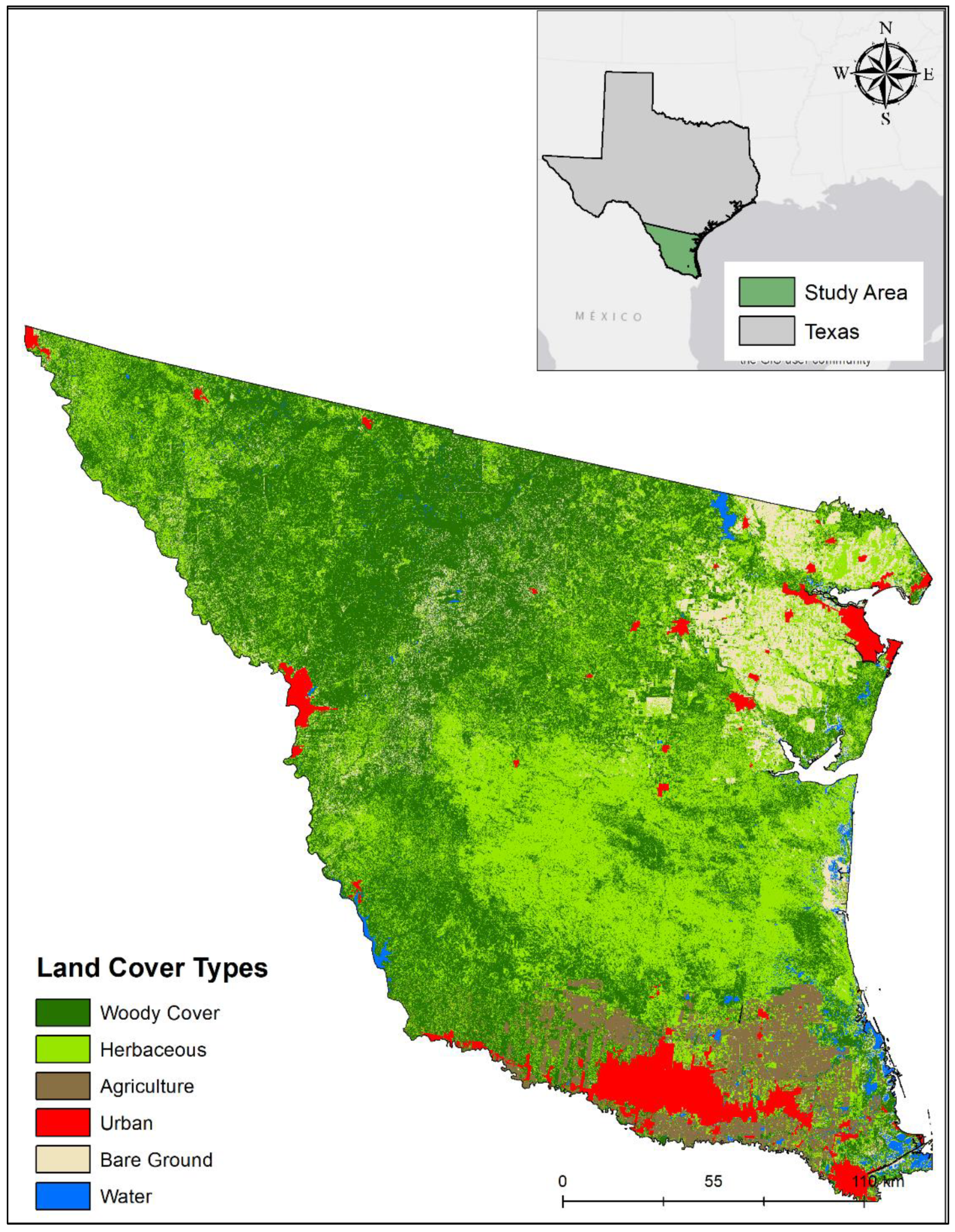
2.1. Study Area

Our study area encompassed 54,170 km² in southern Texas encompassing the Texas-Tamaulipan Thornshrub, Coastal Sand Plain, Lower Rio Grande Valley, Rio Grande Floodplain, Northern Nueces Alluvial Plain, Rio Grande Floodplain and Terraces, Southern Subhumid Gulf Coast Prairie, West Gulf Coast Floodplains and Terraces, and Laguna Madre Barrier Islands and Coastal Marshes eco-regions (Figure 1; [48]). This area includes the counties of San Patricio, Nueces, Kleberg, Kenedy, Willacy, Cameron, Hidalgo, Brooks, Starr, Zapata, Jim Hogg, Jim Wells, Duval, Webb, and parts of Live Oak, McMullen, La Salle, Dimmit, and Maverick counties. These areas have diverse land use types including varying densities of urban development, industrial facilities for oil and natural gas, row-crop agriculture, rangelands for cattle production, as well as natural areas composed of mid-grass prairie, coastal and inland wetlands, inland salt lakes, and a mosaic of diverse woody communities (e.g., live oak forest and thornshrub) [42]. The region has a network of high-speed (80–120 kph) state and county highways (60–80 kph) that increase in density and traffic volume closer to micropolitan and metropolitan areas (i.e., Kingsville, Brownsville, Laredo, Corpus Christi, McAllen) and near the US-Mexico border.

2.2. Ocelot Spatial Data

Data collection occurred in northeastern Willacy and southeastern Kenedy counties. Ocelots were captured on the East Foundation’s El Sauz Ranch; a large working ranch managed to promote the advancement of land stewardship through cattle ranching, science, and education. This has the largest known breeding population of ocelots in the United States [31,37,38]. The ranch is located among a mosaic of expansive private rangelands in Willacy and Kenedy counties.

From March 2013 to May 2017, and March 2019 to May 2020, we captured 20 ocelots (16 adults; 4 juveniles) with single-door, 108 × 55 × 40 cm steel wire Tomahawk (Tomahawk Trap Company, Tomahawk, WI, USA) box traps. We used a pole syringe to sedate adult ocelots with a mixture of zolazepam and tiletamine HCl (Telazol, Fort Dodge Laboratories, Fort Dodge, Iowa, USA) at 5 mg/kg [45] from 2013 to 2017 [38,49]. From 2019 to 2020, we sedated ocelots with a mixture of medetomidine HCl 0.05 mg/kg and ketamine hydrochloride at 4–5 mg/kg and used a reversal of 5 mg of atipamezole per 1 mg medetomidine (ZooPharm, Laramie, WY, USA). Juvenile ocelots were released without being sedated.

We attached Lotek Minitrack or Litetrack global positioning system (GPS) (Lotek Wireless™, Newmarket, ON, Canada) Iridium-satellite collars on 16 adult ocelots (seven males, nine females). We used a variety of temporal fix schedules (based on prior project objectives) to record GPS relocations of ocelots. Following data collection, we removed outlying locations that may have been the result of pre-deployment testing and locations collected within 24 h of capture to minimize bias due to live capture [7,38]. We applied a geographic filter to exclude locations that had a dilution of precision >10 and coverage from less than four satellites and removed geographic outlier locations determined to be erroneous [38]. For this analysis, we split the dataset into historic observed locations (2013 to 2015) and current data (2016 to 2020). To ensure standardization among different fix schedules across datasets, we calculated the Euclidean distance (m) between successive locations and used Pearson’s correlation analysis (significance p = 0.05) to determine the similarity between pairs of successive steps at different temporal intervals [50]. Based on lower temporal autocorrelation among successive locations at two hours, we used ArcMap 10.8 (ESRI, Redlands, CA, USA) to subsample GPS telemetry data every 2 h for further spatial analyses.

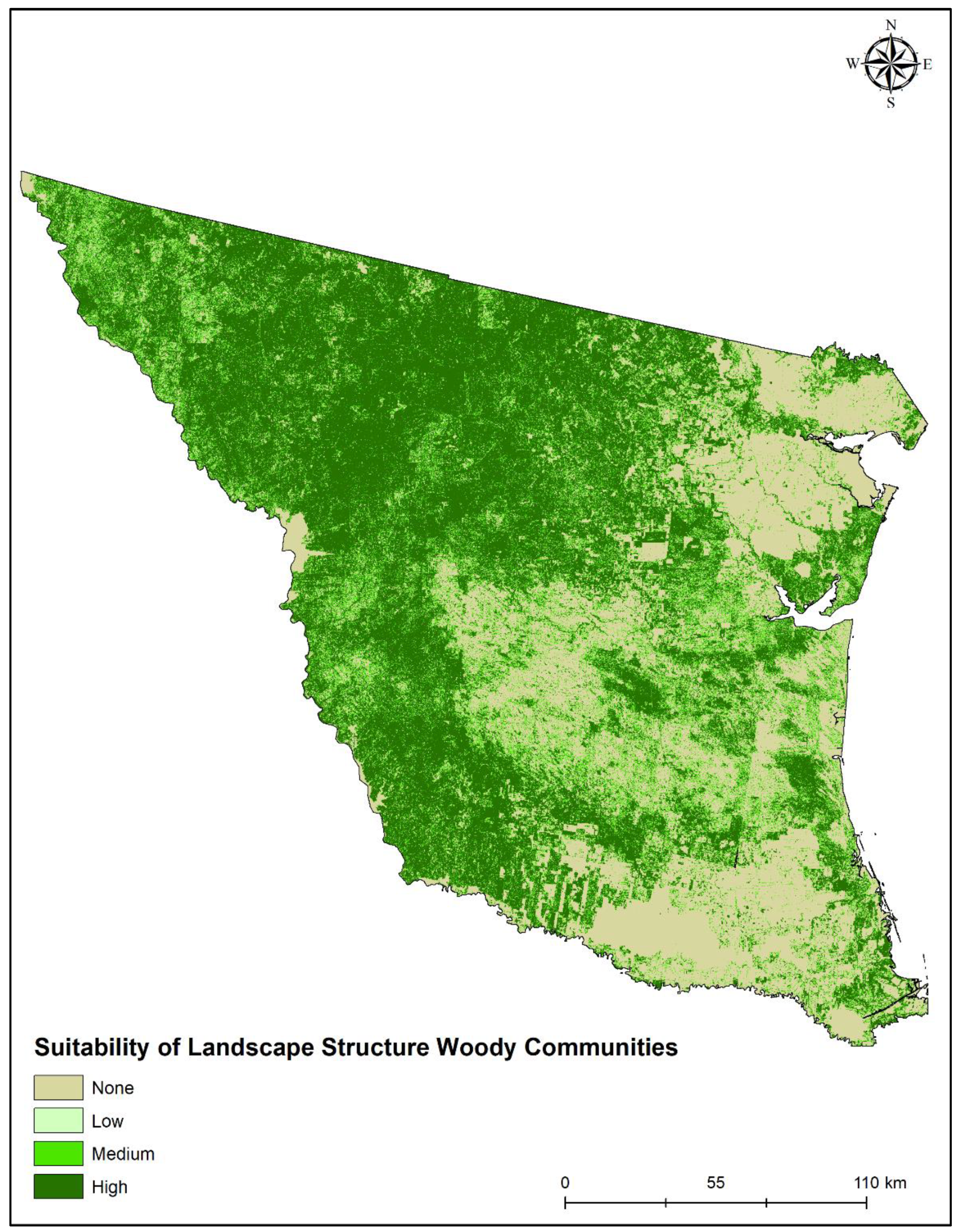
2.3. Landscape Suitability Analyses

We acquired 2018 LANDSAT 8 satellite imagery (30-m) to evaluate the range of landscape structure metrics believed to influence the spatial distribution and structure of woody cover for ocelots across the study area. We acquired five LANDSAT images from March to May 2018 with minimal cloud cover (<10%) through the U.S. Geological Survey Global Visualization Viewer [44,51]. We followed methodologies and classifications defined by Lombardi et al. [44] for classifying land cover types in southern Texas using an unsupervised image classification in ERDAS IMAGINE 2018 (Hexagon Geospatial, Norcross, GA, USA). We defined six land cover classifications including woody cover, herbaceous cover, croplands, water, barren soil, and urban areas (Figure 1). To classify the maximum extent of urban areas, we used spatial data of urban areas obtained from the U.S. Census from the Texas Natural Resource Information System (Texas Natural Resource Information System, Austin, TX, USA), digitized new development, and merged the layers to the unsupervised classification. We performed accuracy assessments for each image using 200 random points using a confusion matrix [31,34,44] that produced a mean 91.9% accuracy for image classifications.

We identified the range of characteristics of woody patches and the landscape vegetation structure used by ocelots based on the 2016–2020 GPS telemetry dataset using the theory of slack (hereafter slack; [52]). Slack introduces the idea that the 90% range of different patch configurations and complexities lead to optimal habitat conditions within a fully usable space [28,52]. Using slack, we defined the range of values for each metric from five to 95 percentiles and reclassified each landscape metric raster into habitat (1) and non-habitat (0) [28,52].

We used Fragstats (Fragstats 4.2, [53]) to obtain landscape metrics of woody cover that have been previously shown to characterize the spatial distribution and structure of woody cover related to ocelot occurrence and space use across their geographic range (including southern Texas) (

Table 1. A priori predictions and justification for landscape metrics of woody cover for inclusion in gradient + slack landscape suitability model for ocelots (Leopardus pardalis) in southern Texas.

Landscape Metric	Prediction	Citation
Landscape Shape Index	Ocelots use a range of values with lower shape values on the landscape	Jackson et al., 2005, Lombardi et al., 2020
Percent Landscape (%)	Ocelots use a range of higher percentage of woody cover on the landscape	Tewes and Everett 1986, Jackson et al., 2005, Haines et al., 2006, Connally 2009, Massara et al., 2018, Paolino et al., 2018, Wang et al., 2019, Lombardi et al., 2020, Blackburn et al., 2020
Patch Density (patches/100 ha)	Ocelots use a range of lower patch densities, indicative of large patches on the landscape	Wang et al., 2019, Blackburn et al., 2020
Largest Patch Index (%)	Ocelots use a range of larger woody patch indices on the landscape	Tewes and Everett 1986, Jackson et al., 2005, Haines et al., 2006, Connally 2009, Massara et al., 2018, Paolino et al., 2018, Wang et al., 2019, Lombardi et al., 2020, Blackburn et al., 2020
Edge Density (m/ha)	Ocelots use a range of lower edge densities, indicative of a forest -interior species on the landscape	Garcia-R et al., 2019
Mean Patch Area (ha)	Ocelots use the largest mean patch areas on the landscape	Jackson et al., 2005, Lombardi et al., 2020, Wang et al., 2019
Aggregation Index	Ocelots use a range of larger aggregation indices on the landscape	Blackburn et al., 2020

) [31,32,33,34,39,40,41,54]. We estimated the size (mean patch size [MPA; ha]), patch density (PD; the number of patches/100 ha), and complexity of woody cover patches (landscape shape index (LSI), which yield an index of patch fragmentation. We examined the aggregation of woody cover patches (aggregation index; AI) and the amount of edge per unit area (edge density (ED; m/ha). We used the largest patch index (LPI; %) to examine the percentage of area covered by the largest patch of woody cover and the total proportion of woody cover (PLAND; %) on the landscape. We then created focal raster layers for each landscape metric and the entire study area using a moving window analysis to address the role of these patterns and processes to a wider extent. To inform these focal raster layers, we calculated focal radii based on the average distance between two successive locations (2 h; 116 m) to derive the range of values for each landscape metric used by ocelots for each pixel across the study area. We quantified descriptive statistics for each landscape metric in SPSS (IBM SPSS v23;). Using the 90% range of values for each metric [51], we reclassified each raster using a classification of nonhabitat (0) and habitat (1) and used a raster calculator to sum the resulting layers into one suitability model of seven metrics. To create the final suitability model, we reclassified this summed raster of seven metrics into four suitability categories: high (6–7 metrics), medium (3–5 metrics), low (1–2 metrics), and none (0 metrics).

2.4. Model Validation

To verify our gradient suitability map, we used ocelot telemetry locations from the historic 2013 to 2015 dataset (n = 6 individual ocelots). Using the extract values-to-point tool in ArcMap 10.8.1, we extracted the expected suitability (none, low, medium, and high) values from observed ocelot locations from the historic dataset and the expected ocelot location data set used to generate the suitability map. We used a chi-squared (χ²) statistical test for significant differences between observed ocelot locations for each year (2013–2015) and expected suitability [55]. If no significant differences were reported, the woody cover suitability model for ocelots may be applicable to be used at different spatio-temporal periods.

3. Results

Landscape metrics associated with woody patches were ED range: 0–551.72 m/ha; MPA range 0–4.60 ha; PD range 0–306.51 patches/100 ha; LSI: 0–3.37 (

Table 2. Summary statistics for defining the optimal range of woody cover conditions for ocelots in southern Texas. Values were derived from moving window analysis and GPS relocations for ocelots. The criterion of suitability scores was representative of the 90% range of values (1) and the bottom 5%, and the top 5% were excluded from analysis (0).

Landscape Metric	Criterion	Score
Landscape Shape Index	0–1.07	0
	1.07–2.25	1
	2.25–3.37	0
Percent Landscape (%)	0–41.3	0
	41.3–100	1
Patch Density (patches/100 ha)	0–22.6	0
	22.7–72.4	1
	72.5–306.5	0
Largest Patch Index (%)	0–34.3	0
	34.4–100	1
Edge Density (m/ha)	0–191.5	1
	191.6–551.7	0
Mean Patch Area (ha)	0–0.86	0
	0.87–4.4	1
Aggregation Index	0–54	0
	55–98	1

). There was a variation of small and large patches of woody cover intermixed across the region (PLAND: 0–100%; LPI range 0–100%; AI: 0–100; Table 2).

Suitable woody cover for ocelots was characterized by a 90% range of small densities of large and naturally shaped patches (PD range: 22.60–72.40 patches/100 ha; MPA range: 0.87–4.40 ha, LSI range: 1.07–2.25), indicating a range of less fragmented patches. Ocelots used a combination of large patches of woody cover (PLAND range: 41.4–100%; LPI range: 34.04–100%; AI range: 55–98%) and a lesser amount of edge per unit area (ED: 0–191.50 m/ha; Table 2). High projected landscape woody suitability for ocelots across southern Texas was 45.27% (24,429.67 km²); medium, 11.42% (6160.52 km²); low, 12.08% (6519.97 km²); and none, 31.23% (16,858.41 km²) (Figure 2). Across our study area, the largest areas of high suitability exist in the northern and southwestern areas (i.e., Texas-Tamaulipan Thornshrub eco-region). We also observed large and isolated highly suitable patches in the eastern mid-coastal areas (i.e., eastern Coastal Sand Plain and upper Laguna Madre Coastal Marsh eco-region) parts of our study area.

Percentage of combined ocelot locations in high suitability cover was 84.8% (observed in this study from 2016 to 2020). We observed variation in the percentage of historical ocelot relocations in high suitable cover (2013: 90.9%, 2014: 64.4%, and 2015: 87.9%). Percentage of ocelot relocations observed in this study in medium and low suitable cover was 6.92% and 4.10% (2016–2020), respectively. Model verification indicated percentages of expected ocelot relocations and observed historical ocelot relocations were not statistically different between 2013–2015, except for 2014 (χ² = 38.6, α = 0.05; df = 3;

Table 3. Chi-square (χ²) analysis for woody cover suitability model verification based on historic ocelot GPS relocations from the East Foundation’s El Sauz Ranch. Recent ocelot GPS relocations from 2016 to 2020 were used in the moving window analysis as the expected dataset for this analysis. Tabulated χ² values > 7.81 (α = 0.05, df = 3) indicate a statistical difference (*) in suitability model and observed location data from ocelots.

Year	High	Medium	Low	None	χ2
Expected	84.8	6.92	4.1	4.18
Observed 2013	90.9	2.2	4.5	2.4	4.42
Observed 2014	65	15.8	13.8	5.4	39.6 *
Observed 2015	87.9	8.1	1.83	6.5	2.85

).

4. Discussion

This study demonstrated a new approach for measuring vegetation cover suitability by applying the gradient concept of landscape structure and slack for developing a landscape suitability model for the endangered ocelot populations in southern Texas. We show that the range of landscape vegetation structure metrics important for ocelot use is composed of low patch densities of large and naturally shaped patches, suggesting forest-dependent species [31,33]. This strengthens growing support for use of landscape metrics in quantifying woody cover patch patterns, configurations, shapes, and densities that may be used by ocelots in Texas [31,32,39,41]. We have combined rigorous advancements in remote sensing and landscape ecological analyses using current relocation data to identify a larger extent of suitable landscape structure of woody cover than previously known. This model also was partially effective in identifying the suitable landscape structure of observed ocelot relocations in high suitability patches of woody cover across years.

Ocelots used a range of conditions that reflected areas containing woody cover that had more naturally shaped patches with extremely low edge densities compared to the surrounding study area, indicating a range representation of non-fragmented areas. Our results are consistent with Garcia-R. et al. [45] who suggested ocelots occurring in the northern Andes Mountains in Colombia had lower indices of occurrence in areas with high edge density of forested cover. Further, some of our findings at 30 m resolution are similar to a recent study by Lombardi et al. [31] at finer spatial resolutions (i.e., 1 m imagery), which is indicative that the range values for mean patch area and landscape shape indices may be consistent across spatial scales.

Increased mean patch area, large patch index, and percentage of woody cover are related to increasing forested cover, which has been widely linked to the occurrence of ocelots throughout their range [31,33,45,54,56]. Preference for large areas of forested cover possibly indicates use for specific behaviors such as for reproduction [57], prey [32,58,59], and may play a key role in facilitating coexistence with competitor species [59,60,61]. In areas of the Atlantic Forest in Brazil, ocelot occurrence has been strongly linked to large patches of undisturbed forest, similar to southern Texas and believed to be rare, particularly in human-modified landscapes [54,61,62]. This study reveals ocelots use a wide range of configurations, complexities, and distribution of woody cover. Ocelots did not exhibit landscape structural specialization, which is consistent with studies in Central and South America [33,45,54,60,61,62].

This model successfully identified the suitable landscape vegetation structure for areas in our study area in which ocelots were observed. We were able to successfully predict observed relocations in high suitable woody cover patches in 2013 and 2015. Observed significant differences detected in 2014 were likely a result of targeted trapping efforts and subsequent ocelot home ranges within a transition zone of extensive wetlands and small-disjointed patches of thornshrub and forest. Our results indicate that the gradient and slack model developed for ocelots has strong predictive ability across time and space. These results can be further refined using ocelot GPS relocation data from adjacent populations in northeastern Mexico and the more fragmented population on the Laguna Atascosa Wildlife Refuge.

Our model also reflects a new standard in estimating the amount of potential woody cover conditions that may be used by ocelots across the study area. Over the last 35 years, advancements in remote sensing approaches (i.e., aerial visual surveys vs. landsat imagery) provide the ability to quantify large regions of woody vegetation with greater accuracy and precision than before. Tewes and Everett [46] using early remote sensing techniques from aerial transects estimated that the southern 13 counties of southern Texas comprised 1.6% of suitable canopy cover for ocelots. An important distinction between the previous study and our methods, is the inclusion of live oak forests (and thornshrub understories), to ensure the full range of woody cover conditions used by ocelots. The inclusion of live oak now yields more potential woody cover with suitable landscape structure of woody cover. Furthermore, these results also indicate the impact of agriculture and urbanization on suitability indices, as suitable patches in the southeastern region of the study area are smaller and more fragmented. Consequently, this model provides a strong framework to also show the impact that human activity (Figure 2) on suitability indices for potentially suitable woody cover for ocelots.

These results contradict findings by Haines et al. [36] and more recently Lehnen et al. [40]) in southern Texas. Haines et al. [36] predicted 11 patches of suitable habitat in the areas where ocelots are known to exist, based solely on canopy cover. Lehnen et al. [40] used GPS data from 2012 to 2017 with coarse (50 m) resampled LiDAR and satellite imagery to predict suitability for ocelots at the second-order (home range; [63]) for each population in Texas. Each study did not account for the potential of ocelots to occur in forested cover in addition to thornshrub and used data from Laguna Atascosa National Wildlife Refuge without forested cover to extrapolate their results across larger areas. Because of our broad woody cover classification, which includes oak forests and thornshrub, we now can report that the forested cover adjacent to and surrounding those previously identified patches in Kenedy and Willacy counties contain high suitable landscape vegetation structure, and include areas with resident ocelot populations (i.e., El Sauz; [31,38]). The presence of ocelots in areas previously deemed unsuitable [36,40,46], and recent research suggesting that dense thornshrub canopy cover may not be the sole factor determining woody cover use by ocelots in Texas, may reflect greater behavioral plasticity by ocelots for mixed canopies in live oak and thornshrub communities than previously believed [31].

Our approach and findings offer opportunities for advancing ocelot recovery and road planning efforts, such as informing recovery mitigation strategies. In Texas, to achieve the first “downlisting” criterion of the Ocelot Recovery Plan, at least 200 ocelots must exist in current populations with a new reintroduced population established within the historic range [37,56]. Our suitability model allows for rapid assessment of other regions outside our study area for future translocation. We project the largest areas for potential reintroduction exist in the extensive northern and southwestern regions of the study area occurring within the Texas-Tamaulipas Thornshrub eco-region and select large patches along the middle coastal areas (i.e., directly north of current ocelot populations), and not in highly urbanized areas near the Texas-Mexico border. However, due to the presence of high-speed (120 kph) roadways bisecting areas with suitable woody cover across southern Texas, we recommend these findings be incorporated into future road planning efforts to ensure dispersal and connectivity among woody patches where there is a reasonable likelihood of resident ocelot populations [64]. These results can also be applied for recovering ocelots in other parts of their geographic range, like Brazilian Atlantic Forest, an area also marked by heavy fragmentation and extensive road networks [54,61,62,65].

We acknowledge that our ocelot GPS dataset derived from a small geographic area and when extrapolating across larger regional areas, we recommend using caution in interpreting results. The landscape suitability map produced in this study projects the potential suitability of woody cover landscape structure based on the range of values used by ocelots and should not be interpreted as a probability map of ocelot occurrence [18,66,67]. These results can be used to develop initial planning steps to identify suitable areas for ocelot habitat. However, they will need to be complemented with incorporation of other finer scale variables that may also influence ocelot distribution such as shrub height and density [68], road density [69], prey availability [59], and climatic variables [10].

5. Conclusions

This approach demonstrates the ability of using the gradient concept and slack to identify suitable landscape structure of woody cover that may help inform conservation strategies for medium-sized felids or carnivores. The transferability and validation of this study are other examples of the importance of incorporating these landscape metrics into examining the landscape structure of vegetative cover in studies on ocelots or other highly mobile medium-sized felids. We recommend these results be incorporated into future ocelot recovery efforts and applied to other threatened and endangered carnivore species.

References

1. Hirzel, A.H.; le Lay, G.; Helfer, V.; Randin, C.; Guisan, A. Evaluating the ability of habitat suitability models to predict species presence. Ecol. Model. 2006, 199, 142–152. [Google Scholar] [CrossRef]
2. Turner, M.G.; Gardner, R.G. Introduction to landscape ecology and scale. In Landscape Ecology in Theory and Practice; Turner, M.G., Gardner, R.G., Eds.; Springer: New York, NY, USA, 2015; pp. 1–32. [Google Scholar]
3. Rondinini, C.; di Marco, M.; Chiozza, F.; Santulli, G.; Baisero, D.; Visconti, P.; Hoffmann, M.; Schipper, J.; Stuart, S.N.; Tognelli, M.F.; et al. Global habitat suitability models of terrestrial mammals. Philos. Trans. R. Soc. B Biol. Sci. 2011, 366, 2633–2641. [Google Scholar] [CrossRef] [PubMed]
4. Guisan, A.; Zimmermann, N.F. Predictive habitat distribution models in ecology. Ecol. Model. 2000, 135, 147–186. [Google Scholar] [CrossRef]
5. Baasch, D.M.; Tyre, A.J.; Millspaugh, J.J.; Hygnstrom, S.E.; Vercauteren, K.C. An evaluation of three statistical methods used to model resource selection. Ecol. Model. 2010, 221, 565–574. [Google Scholar] [CrossRef] [Green Version]
6. Jenkins, J.M.A.; Lesmeister, D.B.; David, R.J. Resource selection analysis. In Quantitative Analyses in Wildlife Science; Brennan., L.B., Tri, A.N., Marcot, B.G., Eds.; Johns Hopkins University Press in Affiliation with The Wildlife Society: Baltimore, MD, USA, 2021; pp. 199–215. [Google Scholar]
7. Poor, E.E.; Scheick, B.K.; Mullinax, J.M. Multiscale consensus habitat modeling for landscape level conservation prioritization. Sci. Rep. 2020, 10, 1–13. [Google Scholar] [CrossRef] [PubMed]
8. Cianfrani, C.; Le Lay, G.; Hirzel, A.H.; Loy, A. Do habitat suitability models reliably predict the recovery areas of threatened species? J. Appl. Ecol. 2010, 47, 421–430. [Google Scholar] [CrossRef]
9. Rondinini, C.; Stuart, S.; Boitani, L. Habitat suitability models and the shortfall in conservation planning for African vertebrates. Conserv. Biol. 2005, 19, 1488–1497. [Google Scholar] [CrossRef]
10. Martínez-Meyer, E.; González-Bernal, A.; Velasco, J.A.; Swetnam, T.L.; González-Saucedo, Z.Y.; Servín, J.; López-González, C.A.; Oakleaf, J.K.; Liley, S.; Heffelfinger, J.R. Rangewide habitat suitability analysis for the Mexican wolf (Canis lupus baileyi) to identify recovery areas in its historical distribution. Div. Distrib. 2021, 27, 642–654. [Google Scholar] [CrossRef]
11. Sanderson, E.W.; Beckmann, J.P.; Beier, P.; Bird, B.; Bravo, J.C.; Fisher, K.; Grigione, M.M.; López-González, C.A.; Miller, J.R.; Mormorunni, C.; et al. The case for reintroduction, the jaguar (Panthera onca) in the United States as a model. Conserv. Sci. Pract. 2021. [Google Scholar] [CrossRef]
12. Hirzel, A.; Guisan, A. Which is the optimal sampling strategy for habitat suitability modeling. Ecol. Model. 2002, 157, 331–341. [Google Scholar] [CrossRef]
13. Guisan, A.; Thuiller, W.; Zimmermann, N.F. Habitat Suitability and Distribution Models, with Applications in R; Cambridge University Press: Cambridge, UK, 2017. [Google Scholar]
14. McGarigal, K.; Cushman, S. The gradient concept of landscape structure. In Issues and Perspectives in Landscape Ecology; Wiens, J.A., Moss, M.R., Eds.; Cambridge University Press: Cambridge, UK, 2005; pp. 112–119. [Google Scholar]
15. Evans, J.S.; Cushman, S.A. Gradient modeling of conifer species using random forests. Landsc. Ecol. 2009, 24, 673–683. [Google Scholar] [CrossRef]
16. Cushman, S.A.; Gutzweiler, K.; Evans, J.S.; McGarigal, K. The gradient paradigm, a conceptual and analytical framework for landscape ecology. In Spatial Complexity, Informatics, and Wildlife Conservation; Cushman, S.A., Huettmann, F., Eds.; Springer: Tokyo, Japan, 2010; pp. 83–108. [Google Scholar]
17. Zemanova, M.A.; Perotto-Baldivieso, H.L.; Dickins, E.L.; Gill, A.B.; Leonard, J.P.; Wester, D.B. Impact of deforestation on habitat connectivity thresholds for large carnivores in tropical forests. Ecol. Proc. 2017, 6, 21–32. [Google Scholar] [CrossRef] [Green Version]
18. Perotto-Baldivieso, H.L. Essential concepts in landscape ecology for wildlife and natural resource managers. In Wildlife Management and Landscapes, Principles, and Applications; Porter, W.F., Parent, C.J., Stewart, R.A., Williams, D.M., Eds.; Johns Hopkins University Press in Affiliation with The Wildlife Society: Baltimore, MD, USA, 2021; pp. 53–67. [Google Scholar]
19. Howery, L.D.; Bailey, D.W.; Laca, E.A. Impact of spatial memory on habitat use. Graz. Livest. Wildl. 1999, 70, 91–100. [Google Scholar]
20. Cagnacci, F.; Boitani, L.; Powell, R.A.; Boyce, M.S. Animal ecology meets GPS-based radiotelemetry: A perfect storm of opportunities and challenges. Philos. Trans. R. Soc. B 2010, 365, 2157–2162. [Google Scholar] [CrossRef] [Green Version]
21. Milleret, C.; Ordiz, A.; Sanz, A.; Uzal, A.; Carricondo-Sanchez, D.; Eriksen, A.; Sand, H.; Wabakken, P.; Wikenros, C.; Åkesson, M.; et al. Testing the influence of habitat experienced during the natal phase on habitat selection later in life in Scandinavian wolves. Sci. Rep. 2021, 9, 1–11. [Google Scholar] [CrossRef] [Green Version]
22. Frazier, A.E.; Wang, L. Modeling landscape structure response across a gradient of land cover intensity. Landsc. Ecol. 2013, 28, 233–246. [Google Scholar] [CrossRef]
23. Hoechstetter, S.; Walz, U.; Xuan, T.N. Effects of topography and surface roughness in analyses of landscape structure, a proposal to modify the existing set of landscape metrics. Landsc. Online 2008, 3, 1–14. [Google Scholar] [CrossRef]
24. Frazier, A.E.; Kedron, P. Comparing forest fragmentation in eastern US forests using patch-mosaic and gradient surface models. Ecol. Inform. 2017, 41, 108–115. [Google Scholar] [CrossRef]
25. Mandal, M.; Nilanjana, D.C. Spatial alteration of fragmented forest landscape for improving structural quality of habitat: A case study from Radhanagar Forest Range, Bankura District, West Bengal, India. Geol. Ecol. Landsc. 2020, 1–8. [Google Scholar] [CrossRef] [Green Version]
26. Moniem, H.E.M.A.; Holland, J.D. Habitat connectivity for pollinator beetles using surface metrics. Landsc. Ecol. 2013, 28, 1251–1267. [Google Scholar] [CrossRef]
27. Hou, W.; Ulrich, W. An integrated approach for landscape contrast analysis with particular consideration of small habitats and ecotones. Nat. Conserv. 2016, 14, 25. [Google Scholar] [CrossRef] [Green Version]
28. Mata, J.M. Landscape-Level Tanglehead Dynamics and the Effects on Northern Bobwhite Habitat. Master’s Thesis, Texas A&M University-Kingsville, Kingsville, TX, USA, 17 December 2017. [Google Scholar]
29. Hunter, L. Carnivores of the World; Princeton University Press: Princeton, NJ, USA, 2019. [Google Scholar]
30. International Union for the Conservation of Nature. The IUCN Red List of Threatened Species. 2020. Available online: http://www.iucnredlist.org (accessed on 14 January 2021).
31. Lombardi, J.V.; Tewes, M.E.; Perotto-Baldivieso, H.L.; Mata, J.M.; Campbell, T.A. Spatial structure of woody cover affects habitat use patterns of ocelots in Texas. Mammal Res. 2020, 65, 555–563. [Google Scholar] [CrossRef]
32. Blackburn, A.; Anderson, C.J.; Veals, A.M.; Tewes, M.E.; Wester, D.B.; Young, J.H.; DeYoung, R.W.; Perotto-Baldivieso, H.L. Landscape patterns of ocelot–vehicle collision sites. Landsc. Ecol. 2020, 17, 1–5. [Google Scholar] [CrossRef]
33. Wang, B.; Rocha, D.G.; Abrahams, M.I.; Antunes, A.P.; Costa, H.C.; Gonçalves, A.L.; Spironello, W.R.; de Paula, M.J.; Peres, C.A.; Pezzuti, J.; et al. Habitat use of the ocelot (Leopardus pardalis) in Brazilian Amazon. Ecol. Evol. 2019, 9, 5049–5062. [Google Scholar] [CrossRef] [Green Version]
34. Satter, C.B.; Augustine, B.C.; Harmsen, B.J.; Foster, R.J.; Sanchez, E.E.; Wultsch, C.; Davis, M.L.; Kelly, M.J. Long-term monitoring of ocelot densities in Belize. J. Wildl. Manag. 2019. [Google Scholar] [CrossRef]
35. Janečka, J.E.; Davis, I.; Tewes, M.E.; Haines, A.M.; Caso, A.; Blankenship, T.L.; Honeycutt, R.L. Genetic differences in the response to landscape fragmentation by a habitat generalist, the bobcat and a habitat specialist, the ocelot. Conserv. Genet. 2016, 17, 1093–1108. [Google Scholar] [CrossRef]
36. Haines, A.M.; Tewes, M.E.; Laack, L.L.; Horne, J.S.; Young, J.H. A habitat-based population viability analysis for ocelots (Leopardus pardalis) in the United States. Biol. Conserv. 2006, 136, 326–327. [Google Scholar] [CrossRef]
37. Tewes, M.E. Conservation Status of the Endangered Ocelot in the United States—A 35-Year Perspective; Texas A&M University-Kingsville: Kingsville, TX, USA, 2019. [Google Scholar]
38. Leonard, J.P.; Tewes, M.E.; Lombardi, J.V.; Wester, D.B.; Campbell, T.A. Effects of sun angle, lunar illumination, and diurnal temperature on temporal movement rates of sympatric ocelots and bobcats in South Texas. PLoS ONE 2020, 15, e0231732. [Google Scholar] [CrossRef]
39. Schmidt, G.M.; Lewison, R.L.; Swarts, H.M. Identifying landscape predictors of ocelot road mortality. Landsc. Ecol. 2020, 35, 1651–1666. [Google Scholar] [CrossRef]
40. Lehnen, S.E.; Sternberg, M.A.; Swarts, H.M.; Sesnie, S.E. Evaluating the population connectivity and targeting conservation action for an endangered cat. Ecosphere 2021, 12, e03367. [Google Scholar] [CrossRef]
41. Jackson, V.L.; Laack, L.L.; Zimmerman, E.G. Landscape metrics associated with habitat use by ocelots in South Texas. J. Wildl. Manag. 2005, 69, 733–738. [Google Scholar] [CrossRef]
42. Leslie, D.M., Jr. An International Borderland of Concern: Conservation of Biodiversity in the Lower Rio Grande Valley; US Geological Survey: Stillwater, OK, USA, 2016. [Google Scholar]
43. Tremblay, T.A.; White, W.A.; Raney, J.A. Native woodland loss during the mid-1900s in Cameron County, Texas. Southwest Nat. 2005, 50, 479–519. [Google Scholar] [CrossRef]
44. Lombardi, J.V.; Perotto–Baldivieso, H.L.; Tewes, M.E. Land cover trends in South Texas (1987–2050): Potential implications for wild felids. Remote Sens. 2020, 12, 659. [Google Scholar] [CrossRef] [Green Version]
45. García, R.S.; Botero-Cañola, S.; Sánchez-Giraldo, C.; Solari, S. Habitat use and activity patterns of Leopardus pardalis (Felidae) in the Northern Andes, Antioquia, Columbia. Biodiversity 2019, 20, 5–19. [Google Scholar] [CrossRef]
46. Tewes, M.E.; Everett, D.D. Status and distribution of the endangered ocelot and jaguarundi in Texas. In Cats of the World: Biology, Conservation, and Management; Miller, S.D., Everett, D.D., Eds.; National Wildlife Federation: Washington, DC, USA, 1986; pp. 147–158. [Google Scholar]
47. Connolly, A.R. Defining Habitat for the Recovery of Ocelots (Leopardus pardalis) in the United States. Master’s Thesis, Texas State University, San Marcos, TX, USA, 2009. [Google Scholar]
48. Griffith, G.; Bryce, S.; Omerik, J.; Rogers, A. Eco-Regions of Texas; Texas Commission on Environmental Quality: Austin, TX, USA, 2007. [Google Scholar]
49. Shindle, D.B.; Tewes, M.E. Immobilization of wild ocelots with tiletamine and zolazepam in southern Texas. J. Wildl. Dis. 2000, 36, 546–550. [Google Scholar] [CrossRef] [Green Version]
50. Perotto-Baldivieso, H.L.; Cooper, S.M.; Cibils, A.F.; Figueroa-Pagán, M.; Udaeta, K.; Black-Rubio, C.M. Detecting autocorrelation problems from GPS collar data in livestock studies. Appl. Anim. Behav. Sci. 2012, 136, 117–125. [Google Scholar] [CrossRef]
51. US Geological Survey Global Visualization Viewer. Available online: https://glovis.usgs.gov/ (accessed on 20 June 2019).
52. Guthery, F.S. Slack in the configuration of habitat patches for northern bobwhites. J. Wildl. Manag. 1999, 63, 245–250. [Google Scholar] [CrossRef]
53. McGarigal, K.; Cushman, S.A.; Neel, M.C.; Ene, E. FRAGSTATS v4.2: Spatial Pattern Analysis Program for Categorical and Continuous Maps. University of Massachusetts. 2015. Available online: http://www.umass.edu/landeco/research/fragstats/fragstats.html (accessed on 15 October 2020).
54. Paolino, R.M.; Royle, J.A.; Versiani, N.F.; Rodrigues, T.F.; Pasqualotto, N.; Krepschi, V.G.; Chiarello, A.G. Importance of riparian forest corridors for the ocelot in agricultural landscapes. J. Mammal. 2018, 99, 874–884. [Google Scholar] [CrossRef]
55. Perotto-Baldiviezo, H.L.; Thurow, T.L.; Smith, C.T.; Fisher, R.F.; Wu, X.B. GIS-based spatial analysis and modeling for landslide hazard assessment in steeplands, Southern Honduras. Agric. Ecosyst. Environ. 2004, 103, 165–176. [Google Scholar] [CrossRef]
56. U.S. Fish and Wildlife Service. Recovery Plan for the Ocelot (Leopardus pardalis), First Revision; Southwest Region, U.S. Fish and Wildlife Service: Albuquerque, NM, USA, 2016. [Google Scholar]
57. Laack, L.L.; Tewes, M.E.; Haines, A.M.; Rappole, J.H. Reproductive life history of ocelots Leopardus pardalis in southern Texas. Acta Ther. 2005, 50, 505–514. [Google Scholar] [CrossRef]
58. Booth-Binczik, S.D.; Bradley, R.D.; Thompson, C.W.; Bender, L.C.; Huntley, J.W.; Harvey, J.A.; Laack, L.L.; Mays, J.L. Food habits of ocelots and potential for competition with bobcats in southern Texas. Southwest Nat. 2013, 1, 403–410. [Google Scholar] [CrossRef]
59. Santos, F.; Carbone, C.; Wearn, O.R.; Rowcliffe, J.M.; Espinosa, S.; Lima, M.G.; Ahumada, J.A.; Gonçalves, A.L.; Trevelin, L.C.; Alvarez-Loayza, P.; et al. Prey availability and temporal partitioning modulate felid coexistence in Neotropical forests. PLoS ONE 2019, 14, e0213671. [Google Scholar] [CrossRef] [Green Version]
60. Nagy-Reis, M.B.; Nichols, J.D.; Chiarello, A.G.; Ribeiro, M.C.; Setz, E.Z. Landscape use and co-occurrence patterns of Neotropical spotted cats. PLoS ONE 2017, 12, e0168441. [Google Scholar] [CrossRef]
61. Cruz, P.; Iezzi, M.E.; de Angelo, C.; Varela, D.; Di Bitetti, M.S.; Paviolo, A. Effects of human impacts on habitat use, activity patterns and ecological relationships among medium and small felids of the Atlantic Forest. PLoS ONE 2018, 13, e0200806. [Google Scholar] [CrossRef]
62. Massara, R.L.; de Oliveira-Paschoal, A.M.; Bailey, L.L.; Doherty, P.F., Jr.; de Frias, B.M.; Chiarello, A.G. Effect of humans and pumas on the temporal activity of ocelots in protected areas of Atlantic Forest. Mamm. Biol. 2018, 92, 86–93. [Google Scholar] [CrossRef]
63. Johnson, D.H. The comparison of usage and availability measurements for evaluating resource preference. Ecology 1980, 61, 65–71. [Google Scholar] [CrossRef]
64. Zeller, K.A.; Wattles, D.W.; DeStefano, S. Evaluating methods for identifying large mammal road crossing locations: Black bears as a case study. Landsc. Ecol. 2020, 35, 1799–1808. [Google Scholar] [CrossRef]
65. Cerqueira, R.C.; Leonard, P.B.; da Silva, L.G.; Bager, A.; Clevenger, A.P.; Jaeger, J.A.; Grilo, C. Potential movement corridors and high road-kill likelihood do not spatially coincide for felids in Brazil: Implications for road mitigation. Environ. Manag. 2021, 67, 412–423. [Google Scholar] [CrossRef]
66. Young, D.; Perotto-Baldivieso, H.L.; Brewer, T.; Homer, R.; Santos, S.A. Monitoring British upland grazing ecosystems with the use of landscape structure as an indicator for state-and-transition models. Rangel. Ecol. Manag. 2014, 67, 380–388. [Google Scholar] [CrossRef]
67. Perotto-Baldivieso, H.L.; Tapaneeyakul, S.; Pearson, Z.J. Using geospatial technologies in wildlife studies. In Wildlife Techniques Manual, 8th ed.; Research: Applications of Spatial Technologies in Wildlife Research; Silvy, N.J., Ed.; Johns Hopkins University Press: Baltimore, MD, USA, 2020; Volume I, pp. 495–510. [Google Scholar]
68. Horne, J.S.; Haines, A.M.; Tewes, M.E.; Laack, L.L. Habitat partitioning by sympatric ocelots and bobcats: Implications for recovery of ocelots in southern Texas. Southwest Nat. 2009, 54, 119–126. [Google Scholar] [CrossRef]
69. Blackburn, A.; Heffelfinger, L.J.; Veals, A.M.; Tewes, M.E.; Young, J.H., Jr. Cats, cars, and crossings: The consequences of road networks for the conservation of an endangered felid. Glob. Ecol. Conserv. 2021, 27, e01582. [Google Scholar] [CrossRef]
Figure 1. The study area for woody cover landscape suitability model for endangered ocelots in southern Texas.
Remotesensing 13 04001 g001
Figure 2. Suitability map of landscape woody cover structure (high (6–7 metrics), medium (3–5 metrics), low (1–2 metrics) none (0 metrics)) for ocelots in southern Texas.
Remotesensing 13 04001 g002