Gap-Filling of NDVI Satellite Data Using Tucker Decomposition: Exploiting Spatio-Temporal Patterns

Abstract

Remote sensing satellite images in the optical domain often contain missing or misleading data due to overcast conditions or sensor malfunctioning, concealing potentially important information. In this paper, we apply expectation maximization (EM) Tucker to NDVI satellite data from the Iberian Peninsula in order to gap-fill missing information. EM Tucker belongs to a family of tensor decomposition methods that are known to offer a number of interesting properties, including the ability to directly analyze data stored in multidimensional arrays and to explicitly exploit their multiway structure, which is lost when traditional spatial-, temporal- and spectral-based methods are used. In order to evaluate the gap-filling accuracy of EM Tucker for NDVI images, we used three data sets based on advanced very-high resolution radiometer (AVHRR) imagery over the Iberian Peninsula with artificially added missing data as well as a data set originating from the Iberian Peninsula with natural missing data. The performance of EM Tucker was compared to a simple mean imputation, a spatio-temporal hybrid method, and an iterative method based on principal component analysis (PCA). In comparison, imputation of the missing data using EM Tucker consistently yielded the most accurate results across the three simulated data sets, with levels of missing data ranging from 10 to 90%.

1. Introduction

The presence of missing data caused by clouds or artifacts in optical satellite data is something that needs to be dealt with in order to obtain a complete time series describing land–surface dynamics.

State of the art algorithms to complete missing information in remote sensing data can be divided into four main categories: Spatial-based, temporal-based, spectral-based, and hybrid methods [1]. Spatial-based methods make use of spatial information to estimate missing data, for example spatial interpolation [2,3], which uses the weighted average of pixels surrounding the missing region [1]. Despite generally being computationally efficient and easy to implement, these methods tend to not perform well when the missing areas cover large heterogeneous regions [4]. Temporal methods utilize data from the same region at different time points. Different temporal replacement methods exist, which can be implemented on a pixel-by-pixel basis [5,6], patch-by-patch [7,8], or on a whole missing region [9,10,11]: Temporal filter methods include sliding window filter methods, which are commonly used to reconstruct normalized difference vegetation index (NDVI) time-series data [12,13,14,15,16] according to some criteria; function-based curve-fitting methods [17,18,19,20]; frequency domain methods [21,22]; and temporal learning based methods [23,24]. Temporal methods tend to perform poorly when the landscape or vegetation changes substantially through dynamical effects due to cloudy conditions or when clouds persist in time and space.

Spectral-based methods are typically multivariate, making up for missing data in one channel by gathering information from the same spatio-temporal unit by using all of the available channels. However, for the optical and thermal range of 400–12,000 nanometers, any missing data in a single channel will result in missing data in all of the channels because clouds are not transparent to radiation at these wavelengths. Wang et al. [25] applied polynomial regression to predict the reflectance of channel 6 of the aqua moderate resolution imaging spectroradiometer (MODIS) sensor, where 15 of the 20 detectors are nonfunctional or noisy channels. This can be useful where one of the channels is malfunctioning due to technical reasons. However, this method cannot be applied to gap-fill for cloudy conditions because clouds are opaque in the optical thermal range, meaning that missing information in one channel will be missing in other channels as well.

Lastly, hybrid methods blend two or more of the above-mentioned categories, combining the strengths of each method with existing examples of implementations including joint spatio-temporal [26,27] and joint spatio-spectral methods [28]. The simplest form of a joint method is to implement two or more of the above-mentioned methods successively, feeding the results of one method into the next algorithm. Sarafanov et al. demonstrate a successful implementation of a successive spatio-temporal method using a machine learning approach [29].

Successive utilization methods do not, however, exploit the existing correlation between different dimensions of the data. Attempts to remedy this include a novel method proposed by Cheng et al. [27] that merges concepts from the spatial and temporal categories, imputing missing data from different spatial locations at different times, assuming that similar groups of neighboring pixels in a given image will have similar dynamics in multitemporal images. Further exploiting the multiway structure of the data by including all modes (dimensions of a tensor, meaning spatial, temporal, and spectral) is however possible with tensor decomposition, a widely used group of algorithms in data mining that is rapidly becoming more relevant and useful with the increasing computational power and storage capabilities of modern computers [30]. A major advantage of tensor decomposition methods is the ability to explicitly take into account the multiway structure of data [30], thereby taking advantage of relationships between pixels in the spatial, spectral, and temporal dimensions. It is well documented that tensor decomposition methods can be used to fill in missing data accurately, even when a large proportion of the data is missing [31,32,33]. The amount of missing data that can be handled while still obtaining accurate results will depend on the tensor decomposition method that is used as well as the structure of the tensor that is decomposed. It has been shown that applications of Tucker decomposition, one of the most widely used methods for gap-filling data in domains other than remote sensing, such as chemometrics [34] or big data for traffic applications [35], can successfully reconstruct noisy tensors with up to 95% missing data [36], but they have not, to our knowledge, been applied to gap-fill time series data from remote sensing data sets at present.

The Iberian Peninsula is a perfect natural laboratory to test gap-filling methods for the remote sensing indices of vegetation greenness due to its large bioclimatic gradients and high seasonal and interannual climatic variations that create dynamic patterns. In addition, land use changes [2,37,38] such as afforestation [39], intensification, aridification, and more frequent forest fires [3,40,41] are prevalent. Given the uncertainty in projected climate change for future decades [42,43], it is crucial to monitor also monitor vegetation changes at a regional scale. These can be accomplished in a cost-effective way by using satellite data. NDVI is a good indicator of changes in vegetation growth and senescence associated with climate and human impacts [44,45,46,47]. The NDVI high-resolution data set from the Iberian Peninsula from Vicente-Serrano et al. [48], which spans 34 years, has been used to assess drought impacts or forest resilience using biweekly composites [49,50,51]. Increasing the temporal resolution to daily time scale can improve biological forecasting by detecting early warning signals of abrupt transitions or ecological thresholds [52,53].

The goal in this study is to assess the performance of expectation maximization (EM) Tucker, a Tucker implementation that iteratively imputes missing data to fill in gaps caused by clouds or low viewing angles in NDVI images from the AVHRR sensor. We used both simulated and real data sets and benchmark the results through comparisons with state-of-the-art methods for gap-filling NDVI time series.

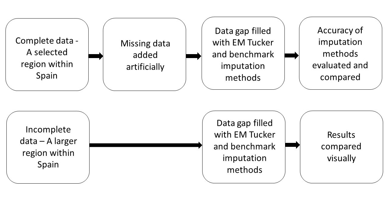
The paper is structured as follows: First, two study regions are introduced followed by an introduction of different gap-filling methods and the performance metrics that we used to compare those methods. Three data sets based on the first study region were established, and missing data were added artificially in order to benchmark the methods. A fourth data set was established based on the second, larger study region. This data set contained natural missing data. We applied all of the methods discussed in an earlier section to this fourth data set in order to demonstrate the application’s performance in a comparative fashion in a real-world situation.

2. Study Region and Data Set

2.1. Study Region

We investigated two separate regions on the peninsula, both of which are within the borders of Spain. The first region (study region 1) is bound by 39°10′N–38°51′N and −2°58′E–2°36′E and primarily consists of forested land, pastures, and cropland. There are no large bodies of water within the region. The second region (study region 2) is located further south and is bound by 36°56′N and 36°45′N and −3°58′E and −2°37′N. This is a larger and more diverse region and includes the greenhouse covered region in the plains of Campo de Dalías in the south-east, the Sierra Nevada mountain range, a few bodies of water as well as shrublands, small forests, and croplands to the north and west. The two study regions were identified by selecting spatial subsets from the Iberian Peninsula after a screening process looking for sites with enough spatial variability driven by different land cover types. An additional criterion for study region 1 was that it needed to contain as little missing data as possible. Observations of the Iberian Peninsula over the course of the chosen time frame are shown in Figure 1. Study regions 1 and 2 are indicated by black rectangles. In addition, Figure 2 shows enlarged plots of the two rectangles.

2.2. Data Sets and Pre-Processing

The Iberian data set consists of daily AVHRR images taken between 1981 and 2015 and encompasses Portugal, Spain, Gibraltar, Andorra, and a small part of Southern France.

The data were acquired from the satellites NOAA-7, -9, -11, -14, -16, -18, and -19 at a spatial resolution of 1.2 km. Daily images were subject to processing that included calibration and cross-calibration, geographical matching, cloud cover removal, top-of-the-atmosphere reflectance calculation, and topographical correction. Details of the processing procedure can be found in [48]. Daily red and infrared reflectance were used to calculate the NDVI index.

Daily NDVI data are available for the entire time period between 1989 and 2015. However, we only used data from a single year (2008), as we assumed that the temporal patterns would be redundant across several years and because we wanted to demonstrate that the method is also applicable to real-world scenarios where less data are available.

The reduced data set (2008) consists of 366 images, each of which contains 1115 × 834 pixels. A large part of the frames is empty, and the remaining ones indicate some degree of missing data. The missing data are the result of prior artifact removal, which was applied to cope with heavy cloud cover, high view angles, or because the images were damaged in some way. Overall, missing data constitute 90% of the data set. There are 215 time frames that contain no data at all. Disregarding these empty frames as well as the ocean (see the estimated shoreline in Figure 1f), the amount of missing data drops to 56%. After removing frames that contain very little or no data, 66 frames remained, resulting in a multiway array of 1115 horizontal × 834 vertical × 66 temporal pixels. Examples of five chosen time frames with various levels of missing data can be seen in Figure 1.

To quantitatively assess the performance of the gap-filling methods, it was necessary to have ground truth values. This is not possible when data are missing due to clouds unless ground sensors are available. To overcome this, we used study region 1, which contained little missing data in order to create three different data sets, namely SIM1, SIM2, and SPAIN1. These were used for model evaluation. Study region 2 contained natural missing data and was used to create a fourth data set, namely SPAIN2, which was used to demonstrate how the gap-filling methods function when applied to a larger area. An overview of all of the data sets is shown in

Table 1. An overview of all data sets used in this study. The resulting data sets will be referred to by the corresponding aliases.

Alias	Description	Dimension
SIM1	Constructed by repeating a single time frame from study region 1 with no missing data. Missing data were added artificially. Used for model evaluation.	30 × 30 × 30
SIM2	Constructed by adding noise to SIM1. Missing data were added artificially. Used for model evaluation.	30 × 30 × 30
SPAIN1	All time frames from study region 1 with no missing data. Missing data were added artificially. Used for model evaluation.	30 × 30 × 54
SPAIN2	Study region 2 with natural missing data. No ground truth data available. Used to demonstrate the performance of the models visually.	90 × 90 × 66

.

The purpose of the simulated time series data sets (SIM1-2) was to conduct a proof-of-concept study under well controlled conditions. The real time series data sets (SPAIN1-2), on the other hand, were used to demonstrate performance with real imagery. SIM1, SIM2, and SPAIN1 were used to evaluate the algorithms with different levels of artificially added missing data. The fourth data set, SPAIN2, was used to demonstrate the application of the algorithms to a larger area (11,660 km²) of the Iberian Peninsula. Thus, for SPAIN2, the actual ground truth values were not known.

The simulated data sets were constructed using the methods described as follows: For SIM1, a single time frame (23 January) was selected from study region 1, as indicated by the small black rectangle in Figure 1. This time frame was replicated 30 times, as shown in Figure 3. All 30 frames in SIM1 were completely identical. To construct the data set, SIM2 gaussian noise with a mean µ = 0 and standard deviation σ = 0.02 was added to all of the SIM1 pixels.

For SPAIN1, study region 1, which contained an overall low amount of missing data, was selected (upper rectangle in Figure 1). All of the time frames indicating missing data were removed. The dimensions for all of the aforementioned data sets are shown in Table 1. A selected number of time frames from SPAIN1 are shown in Figure 4.

Missing data were added to SIM1, SIM2, and SPAIN1 in two different ways. First, pixels were removed completely at random (MCAR) until the missing data reached a desired percentage of elements. Secondly, pixels were randomly removed in 5 × 5 blocks at a time, resulting in data that were missing at random (MAR). The levels of missing data that were analyzed were 0%, 1%, 2.5%, 5%, 10%, 20%, 30%, 40%, 50%, 60%, 70%, 80%, 90%, 95%, and 99%. Examples of three levels of missing data are shown in Figure 5.

In the Iberian data set, the distribution of the missing data appears to be MAR due to the fact that clouds would typically cover patches of land, leading to block-wise missing data. The addition of missing data was conducted a number of times in order to generate data sets that could indicate different levels of missing data in order to evaluate how this aspect would affect the gap-filling performance of the algorithms.

The geographic area of the SPAIN2 data set is shown in Figure 1 and is indicated by the lower rectangle (study region 2). The SPAIN2 dimensions were 90 × 90 × 66 pixels. As the ground truth values were not known, SPAIN2 was solely used to demonstrate the application of EM Tucker for the gap-filling of a larger area. Results are presented and compared to four reference methods by visual means only.

3. Methods

Throughout this paper, tensors will be denoted using upper-case calligraphic letters, matrices and vectors will be denoted using bold, scalars will be denoted using lower-case letters, and matrix or tensor dimensions will be denoted using upper-case letters.

3.1. Tucker Decomposition

Tensors, or multiway arrays, are higher-order generalizations of vectors and matrices. Each dimension of a tensor is called a mode. A matrix is a second order (or two-way) tensor indicating two modes, referring to rows and columns. A third order tensor has three modes, referring to rows, columns, and so-called tubes. As a consequence, matrices store data in “tables”, while third order tensors store data in “boxes”. We will denote third order tensors as ${\mathcal{X}}^{I\times J\times K}$, where I corresponds to the number of rows or horizontal pixels, J corresponds to the number of columns or vertical pixels, and K corresponds to the number of tubes or frames. Using this notation, the data sets that were previously introduced can be denoted as ${\mathcal{X}}_{SIM1}^{30\times 30\times 30}$ for SIM1, ${\mathcal{X}}_{SIM2}^{30\times 30\times 30}$ for SIM2, ${\mathcal{X}}_{SPAIN1}^{30\times 30\times 54}$ for SPAIN1, and ${\mathcal{X}}_{SPAIN2}^{90\times 90\times 66}$ for SPAIN2 in tensor form.

Formally, Tucker decomposes a three-way tensor ${\mathcal{X}}^{I\times J\times K}$ into the three loading matrices $A^{I\times P}$, $B^{J\times Q}$, $C^{K\times R}$ and a core tensor ${\mathcal{G}}^{P\times Q\times R}$, where P, Q, and R denote the ranks in the respective modes (see Figure 6) [54,55]. The rank of a given mode can be understood as the number of independent loading vectors that are necessary in that mode to reconstruct the systematic variation in $\mathcal{X}$. The decomposition is described element-wise in Equation (1).

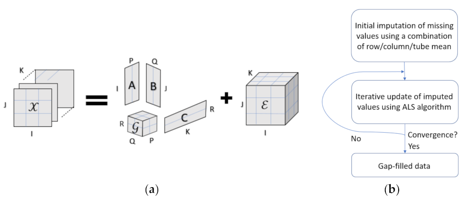
Figure 6. A visual representation of the Tucker decomposition (a). The third order tensor $\mathcal{X}$ is decomposed into a core tensor $\mathcal{G}$ and the loading matrices A, B, and C. The residuals are represented with $\mathcal{E}$, a tensor that is the same size as $\mathcal{X}$. The Tucker decomposition allows for different ranks along the tensor modes, which are denoted as P, Q, and R. The imputation process of EM Tucker is described in (b).

Figure 6. A visual representation of the Tucker decomposition (a). The third order tensor $\mathcal{X}$ is decomposed into a core tensor $\mathcal{G}$ and the loading matrices A, B, and C. The residuals are represented with $\mathcal{E}$, a tensor that is the same size as $\mathcal{X}$. The Tucker decomposition allows for different ranks along the tensor modes, which are denoted as P, Q, and R. The imputation process of EM Tucker is described in (b).

$$x_{ijk}={\sum }_{p=1}^P{\sum }_{q=1}^Q{\sum }_{r=1}^R{a}_{ip}{b}_{jq}{c}_{kr}{g}_{pqr}+e_{ijk}$$

(1)

where $x_{ijk}$ represents a pixel at the i-th row, the j-th column, and the k-th tube of the tensor $\mathcal{X}$. Alternatively, the Tucker decomposition can be formulated using matrix notation, as shown in Equation (2):

$$X_{\left(1\right)}=A{G}_{\left(1\right)}{\left(C\otimes B\right)}^T+E_{\left(1\right)}$$

(2)

where ⊗ denotes the Kronecker product, and $X_{\left(1\right)}$ is the matricized tensor $\mathcal{X}$ across the first mode, as defined by Equation (3).

$${\mathcal{X}}^{I\times J\times K}\to X_{\left(1\right)}^{I\times JK}$$

(3)

The objective of the Tucker model is to minimize the reconstruction error determined via the following loss function equation, Equation (4), where $\parallel ·{\parallel }_F^2$ represents the squared Frobenius norm.

$$\mathrm{L}\left(A,B,C\right)=\Vert X_{\left(1\right)}-A{G}_{\left(1\right)}{\left(C\otimes B\right)}^T{\Vert }_F^2=\Vert E_{\left(1\right)}{\Vert }_F^2$$

(4)

Here, $E_{\left(1\right)}$ represents the residual tensor matricized across its first mode. The objective is most commonly achieved through the use of the alternating least squares algorithm (ALS), which updates the estimates of the loading matrices A, B, and C and the core tensor $\mathcal{G}$ in an iterative fashion, as shown in Equations (5)–(8).

$$A\leftarrow X_{\left(1\right)}{\left(G_{\left(1\right)}{\left(C\otimes B\right)}^T\right)}^{†}$$

(5)

$$B\leftarrow X_{\left(2\right)}{\left(G_{\left(2\right)}{\left(C\otimes A\right)}^T\right)}^{†}$$

(6)

$$C\leftarrow X_{\left(3\right)}{\left(G_{\left(3\right)}{\left(B\otimes A\right)}^T\right)}^{†}$$

(7)

$$\mathcal{G}\leftarrow \mathcal{X}{\times }_1{A}^{†}{\times }_2{B}^{†}{\times }_3{C}^{†}$$

(8)

where ${\left(·\right)}^{†}$ denotes the Moore–Penrose inverse, and ${\times }_n$ is the so-called n-mode product indicating the following property, see Equation (9):

$$\mathcal{X}{\times }_{1}A=\mathcal{Z} such that Z_{\left(1\right)}=A{X}_{\left(1\right)}$$

(9)

In the present context, the intuition behind the Tucker decomposition can be understood as the desire to find a linear combination of outer vector products between the spatial loading vectors in B and C in order to form “factor landscapes”, which are then scaled by scores in A to reconstruct the original data as accurately as possible. Because of this, the spatial loading vectors in B and C can interact or “cross-talk”. The interaction pattern of these loading vectors is encoded in the core tensor $\mathcal{G}$. An illustrative overview of the EM Tucker decomposition as well as a flowchart describing the imputation process is provided in Figure 6.

3.2. EM Tucker for Imputation of Missing Values

The loading matrices A, B, and C are typically initialized using higher order singular value decomposition (HOSVD) [30]. However, HOSVD cannot be used directly in the presence of missing data, as the loss cannot be determined; therefore, prior imputation or marginalization is required. In this study, the imputation approach is chosen, which entails replacing missing data with sensible values before the Tucker decomposition can be applied. One example of a comprehensive imputation approach includes the expectation maximization (EM) algorithm [56], which assumes normal distribution, equal variance, and independence of the residuals.

To gap-fill missing data, we applied EM Tucker, which can be understood as a modification of the Tucker algorithm, such that the iterative imputation of missing values is possible during the ALS fitting procedure [31]. In particular, Equations (5)–(8) are applied to a tensor $\tilde{\mathcal{X}}$, which is defined such that

$${\tilde{\mathcal{X}}}^{\left(s\right)}=\mathcal{X}\ast \mathcal{Y}+{\mathcal{M}}^{\left(s\right)}\ast \left(1-\mathcal{Y}\right)$$

(10)

where ∗ denotes the element-wise product, 1 denotes a tensor containing ones, ${\mathcal{M}}^{\left(s\right)}$ denotes the so-called interim model reconstruction at iteration s, and $\mathcal{Y}$ is a tensor containing elements $y_{ijk}$ such that

$$y_{ijk}=\left\{\begin{array}{l}0 if |x_{ijk } missing\\ 1 if |x_{ijk } not missing\end{array}\right.$$

(11)

Using this procedure, the imputed values are updated at each ALS iteration by using the interim model ${\mathcal{M}}^{\left(s\right)}$. This resembles the maximization step. To incorporate the updated tensor ${\tilde{\mathcal{X}}}^{\left(s\right)}$, the loss function is modified with respect to Equation (10), such that

$$\mathrm{L}\left(A^{\left(s\right)},B^{\left(s\right)},C^{\left(s\right)}\right)=\Vert {\tilde{X}}_{\left(1\right)}^{\left(s\right)}-A^{\left(s\right)}{G}_{\left(1\right)}^{\left(s\right)}{\left(C^{\left(s\right)}\otimes B^{\left(s\right)}\right)}^T{\Vert }_F^2$$

(12)

The loss calculation hereby represents the expectation step of the EM algorithm. Initial imputations for ${\tilde{\mathcal{X}}}^{\left(0\right)}$ are obtained via a combination of row and column means from the matricized tensor. This is completed prior to the initialization of the EM Tucker algorithm [57].

3.3. Model Selection

Decisions needed to be made in order to select the appropriate ranks—or number of components—across the three different tensor modes for the Tucker decomposition. Generally speaking, the reconstruction error will decrease as the number of components increases. However, this will eventually lead to the overfitting of the data, which could result in the potential loss of accuracy when gap-filling any missing data. Strategies for choosing the correct number of components include cross validation strategies as well as the application of so-called information criteria, such as the akaike information criterion (AIC) or the Bayesian information criterion (BIC). Atkinson et al. use these methods to estimate the performance of different models that were applied to NDVI time series data [58].

However, due to the fact that ground truth data are not available for the missing data, AIC and BIC were deemed inadequate to select the optimal number of components across the tensor modes. Instead, we have chosen an alternative model selection strategy that relies on the knowledge of the land-use types of the site. In the following we support our decision through some initial investigations.

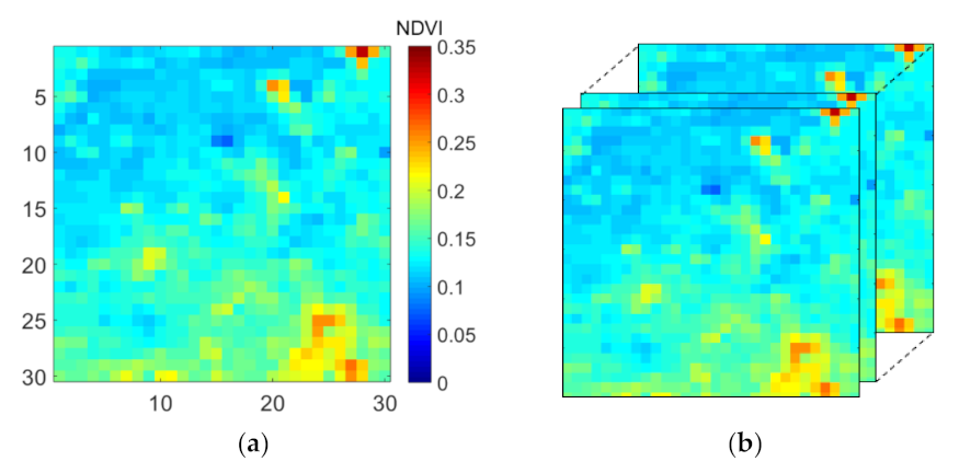
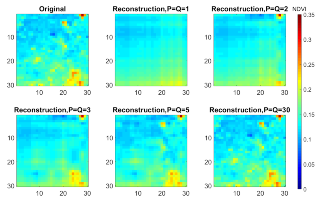
We repeatedly decomposed SIM1 (without missing data) using EM Tucker using different ranks across the spatial modes, P and Q, while assuming the rank across the time mode to be one (R = 1). The model reconstructions for a single time frame obtained for the different spatial ranks can be seen in Figure 7. It appears that the model reconstruction was not accurate when choosing the low ranks across the spatial modes, i.e., the spatial details were not fully recovered. It is noteworthy that the SIM1 tensor did not contain any noise. Hence, we expected to obtain a perfect reconstruction given that our model should capture the systematic variation in the data. We could further see that the reconstruction improved when increasing the spatial ranks. We concluded that the maximal rank was necessary across the spatial modes to obtain accurate data reconstructions. Therefore, P and Q were set to 30 for all Tucker decompositions.

The time mode rank (R), on the other hand, can be understood as the number of independent temporal profiles in the spatial data. For SIM1 and SIM2, we know that all of the time frames contained exactly the same spatial information. Therefore, we chose R = 1 to accurately reconstruct the systematic variation in these tensors. Stated in other words, there is only one independent temporal profile, i.e., all of the pixel values change jointly across the different frames.

However, when looking at SPAIN1, we could find two independent temporal patterns in the data. This is because the region consists of two different land cover types that varied from each other independently of time. We therefore applied a time mode rank R = 2 to model the systematic variations referring to the two sub-regions within the SPAIN1 data set.

In conclusion, we noted that more temporal components would be required if more independent temporal changes were present in the data. This would be the case when trying to gap-fill many very large areas at once using Tucker. However, this is not advisable due to the fact that decomposing large tensors would require considerably high amounts of computational resources, such as computer memory. To mitigate this problem, we limited the geographic size of the tensors and suggested that larger areas, such as SPAIN2, be gap-filled in an iterative fashion. If subsets are chosen to be sufficiently small enough, a low rank can be assumed in the time mode.

To demonstrate this iterative gap-filling procedure, we divided SPAIN2 into nine sub-regions yielding nine tensors of reduced dimensionality, each indicating 10 horizontal pixels × 10 vertical pixels × 52 time points. EM Tucker decompositions were conducted separately for all of the nine tensors.

The selected number of time mode components, R, for the nine EM Tucker decompositions of the SPAIN2 data set were 5, 5, 2, 2, 4, 4, 5, 2, and 4 when counting from top-left to bottom-right in a column-wise fashion. The reasoning behind choosing these ranks were the following: For the EM Tucker decomposition of SPAIN1, we applied R = 2 because we knew about the occurrence of two independent temporal patterns. The subsequent reconstruction of SPAIN1 (with 15% of the missing data) using the obtained Tucker model resulted in 75% of the explained variance among the non-missing pixels. Given the results from this real-world data set, we defined a threshold of 75%, meaning that for the application of the method to new data sets, then number of time mode components that are necessary to explain at least 75% of the variance among the non-missing pixels must be selected.

3.4. Metrics

To evaluate the gap-filling accuracy, the difference between the reconstructions and the original tensors needed to be estimated for SIM1, SIM2, and SPAIN1. This was completed using the relative root mean square error (RRMSE), which is the root mean squared error (RMSE) where data is missing, as shown in Equation (13), divided by the mean of the original tensor, see Equation (14). The overall sum of the elements in the tensor $\mathcal{X}$, ${\sum }_i^I{\sum }_j^J{\sum }_k^K{x}_{ijk}$, was re-written as ${\sum }^{\mathcal{X}}{x}_{ijk}$.

$$RMSE=\sqrt{\frac{1}{{\sum }^{\mathcal{Y}}(1-y_{ijk})}{\sum }^{\mathcal{X}}{\left(x_{ijk}^{Pred}-x_{ijk}\right)}^2\left(1-y_{ijk}\right) }$$

(13)

$$RRMSE=\frac{RMSE}{\overline{x}}$$

(14)

As a second metric, the correlation coefficient between the original tensor and the reconstructed tensor was used. A correlation coefficient close to 1 suggests accurate reconstructions/imputation of the missing data. Only the tensor elements where data were missing were taken into account. The correlation coefficient $r^{3D}$ was calculated as an average across all time frames, as seen in Equation (16). The average predicted value per k-th frame, ${\overline{x}}_k^{Pred}$, was calculated as described in Equation (15).

$${\overline{x}}_k^{Pred}=\frac{1}{{\sum }_i{\sum }_j(1-y_{ijk})}{\sum }_i{\sum }_j{x}_{ijk}^{Pred}(1-y_{ijk})$$

(15)

$$r^{3D}=\frac{1}{K}{\sum }_k\frac{ {\sum }_i{\sum }_j(1-{\mathrm{y}}_{ijk})(x_{ijk}-{\overline{x}}_k)(x_{ijk}^{Pred}-{\overline{x}}_k^{Pred})}{\sqrt{({\sum }_i{\sum }_j(1-{\mathrm{y}}_{ijk}){(x_{ijk}-{\overline{x}}_k)}^2)( {\sum }_i{\sum }_j(1-{\mathrm{y}}_{ijk}){(x_{ijk}^{Pred}-{\overline{x}}_k^{Pred})}^2)} }$$

(16)

The structural similarity index (SSIM) [59] is a third metric that was utilized in this paper to better account for spatial differences between the original tensors and the reconstructed ones. A SSIM of 1 indicates the highest and 0 represents lowest possible structural similarity between images. Unlike previous metrics, SSIM takes into account both elements where missing data were present and where they were not. The tensor mean $\overline{x}$ and standard deviation ${\sigma }_x$ are defined as shown in Equations (17) and (18).

$$\overline{x}=\frac{{\sum }^{\mathcal{X}}{x}_{ijk}}{N}$$

(17)

$${\sigma }_x=\sqrt{\frac{{\sum }^{\mathcal{X}}(x_{ijk}-\overline{x})}{N}}$$

(18)

where N represents the number of elements in tensor $\mathcal{X}.$ SSIM was then calculated in the following way:

$${\sigma }_{x{x}^{Pred}}=\frac{{\sum }^{\mathcal{X}}(x_{ijk}-\overline{x}){ \sum }^{x^{Pred}}(x_{ijk}^{Pred}-{\overline{x}}^{Pred} )}{N}$$

(19)

3.5. Reference Methods

Table 2. An overview of all imputation methods applied in this project.

Alias	Description	Software
Single mean imputation	Tensor mean imputed for missing values	No external code used
Single imputation Tucker (SI Tucker)	Tensor mean was imputed for missing values prior to decomposition	“tucker” function, N-Way Toolbox, Matlab [54]
Hybrid method	Running-window temporal imputation. Remaining missing data then imputed with KNN	“knnimpute” function, Bioinformatics toolbox, Matlab [63]
EM PCA	Column mean was imputed prior to iterative PCA decomposition	“imputeEM” function, mvdlab package, R [55]
EM Tucker	A combination of row and column mean was imputed prior to iterative decomposition	“tucker” function, N-Way Toolbox, Matlab [54]

provides an overview of all of the imputation methods that were applied to gap-fill the four data sets. In particular, four different reference methods were chosen to benchmark the gap-filling performance of EM Tucker, namely a simple mean imputation, single imputation Tucker, EM PCA, and a hybrid method. Hereby, the simple mean imputation method served as a baseline for the comparison, as it simply replaced all of the missing elements with the tensor mean ${\overline{x}}^{*}$. As such, the tensor mean was calculated by only taking into account elements where data were not missing, as denoted in Equation (20).

$${\overline{x}}^{*}=\frac{1}{{\sum }^{\mathcal{Y}}{y}_{ijk}}{\sum }^{\mathcal{X}}{x}_{ijk}{y}_{ijk}$$

(20)

For single imputation Tucker (SI Tucker from here on), all missing elements were initially replaced using the tensor mean, as seen in Equation (20). Subsequently, a Tucker decomposition was performed on the dense tensor. In contrast to EM Tucker, the initial imputations of the missing elements were not updated during the ALS fitting procedure. The optimal number of components were chosen in a similar manner as the one described for EM Tucker (Section 3.3).

EM PCA is a two-way matrix decomposition. To facilitate the decomposition, the tensor was matricized, and PCA was applied to the resulting I × JK matrix using an EM algorithm [60]. The optimal number of PCA components varied between one and two components for SIM1, SIM2, and SPAIN1. For SPAIN2, the optimal component numbers were determined in a similar fashion as the one described for EM Tucker (Section 3.3).

Finally, performance of EM Tucker was compared to a hybrid spatio-temporal imputation method using a sliding time window. Its components are a temporal-based method that estimates missing pixels by calculating the average pixels in the same spatial location from the closest time frames where that information was available. For this analysis, a window size of six was used. When none of the six nearest time frames contained data in the same spatial location of the missing pixel, the missing data were filled using a spatial method, namely K Nearest Neighbors (KNN). This gradually happened more frequently, as the percentage of missing data increased. The KNN algorithm imputed the missing data using the corresponding value from the nearest neighbor column of the IJ x K matricized tensor. This procedure failed when all of the pixels in a time frame were missing.

We used Matlab (version 2017b) [61] and R (version 4.0.3) [62] during this study. The specific packages used for the imputations are stated in Table 2.

4. Results

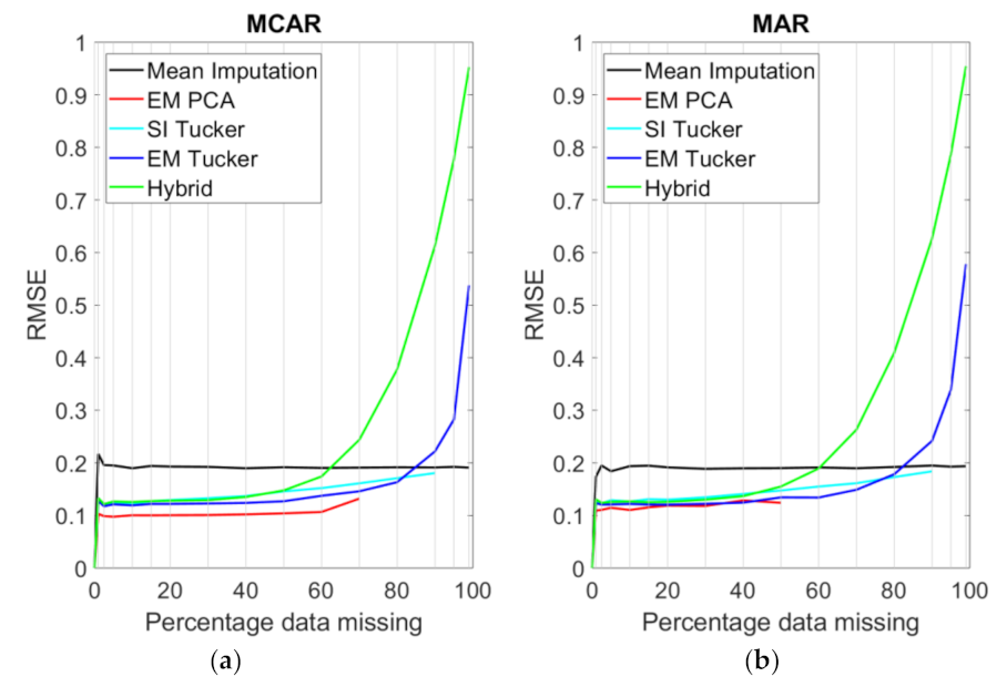
Gap-filling accuracies for the SIM1 data set are shown in Figure 8, with the X-axis showing the percentage of missing data. For this simulation, low RRMSE’s were expected because the data simply consisted of identical frames. If a pixel was missing in one frame, the same information was available in at least one of the other 29 frames for reasonably low levels of missing data. The results reflect this expectation. All of the models indicated no error when 0% of the data were missing due to the fact that only missing pixels were considered during the RRMSE calculation. EM Tucker could reconstruct the tensor close to perfectly in the MCAR case with up to 80% data missing. The EM PCA algorithm failed when the missing data exceeded 70% in the MCAR case and 50% in the MAR case. This can be explained by the fact that no column means could be determined when entire columns of the matricized array were missing. For the EM PCA algorithm, this step was important in order to impute missing elements before iterative imputation was conducted.

The RRMSE for the SI Tucker model appeared to grow approximately linearly as the amount of missing data was increased and approached the level of the EM Tucker for both conditions, MCAR and MAR, as the missing data reached high levels of around 90%. EM PCA consistently performed worse than both EM Tucker and single imputation Tucker. All of the models outperformed the simple mean imputation baseline method, significantly except for EM Tucker when 95% of the or more was missing, and the hybrid method when the level was above 70%. The performance of the hybrid method was approximately on par with EM Tucker in the MCAR case for low levels of missing data but was outperformed by EM Tucker for levels of missing data above 40%. In the MAR case, the hybrid method also performed on par with EM Tucker for the same low levels of missing data, and it even outperformed EM Tucker slightly for MAR at 1–10% and MCAR 1–20%.

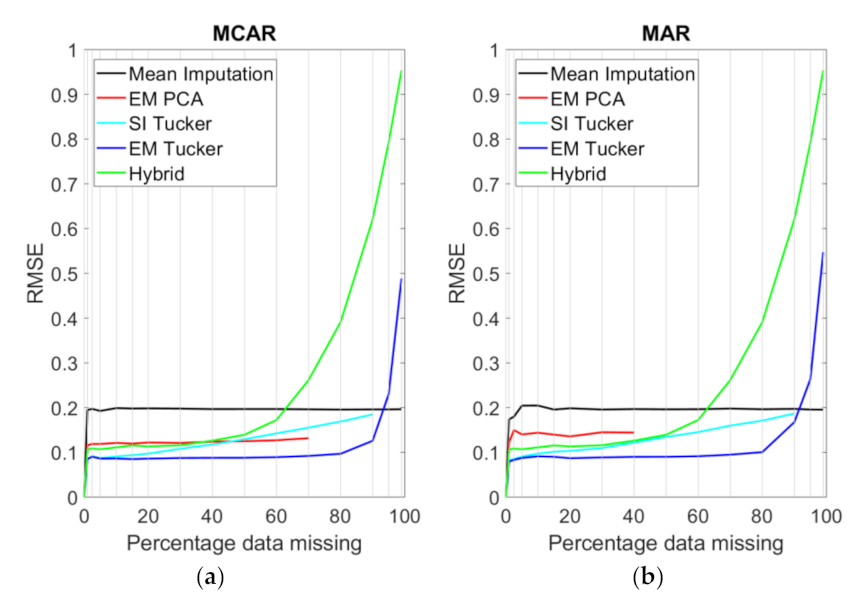
In the case of SIM2, Gaussian noise was added to the homogenous tensor, and all models performed significantly worse, except for EM PCA, which returned similar error levels as it did prior to adding noise. This puts the EM PCA imputation performance approximately on par with EM Tucker for the MAR case, and it outperformed EM Tucker in the MCAR case for all levels of missing data. These results are shown in Figure 9. The hybrid method was outperformed by single imputation Tucker at 50% levels of missing data for both cases, and it was outperformed by the simple mean imputation method, where the missing data exceeded 60%. Interestingly, EM Tucker was outperformed by both the mean imputation method and single imputation Tucker for levels of missing data higher than 80%.

The results for the same models applied to SPAIN1, the subsection of the Iberian data set, are shown in Figure 10. As expected, the resulting error rate was higher for all data completion methods in comparison to SIM1. This was expected, especially when considering the fact that SPAIN1 had higher variability in time and space than SIM1. On the other hand, the error rates were comparable to the ones obtained from SIM2. Notably, for SPAIN1, EM Tucker yielded the lowest RRMSE for all levels of missing data up to 90% for MCAR and up to 95% for MAR. The EM PCA imputation performed significantly worse compared to the other methods. However, it outperformed the hybrid method, where more than 40% of the data were missing, but the algorithm broke when the missing data reached 70% and 40% for MCAR and MAR, respectively. Single imputation Tucker outperformed the hybrid method when more than 50% of the data were missing, but it never matched the performance of EM Tucker.

Evidently, EM Tucker was capable of reconstructing the tensor accurately, even when only fractions of the data remained, with a RRMSE of 12.6% (MCAR) and 16.8% (MAR) for 90% missing data.

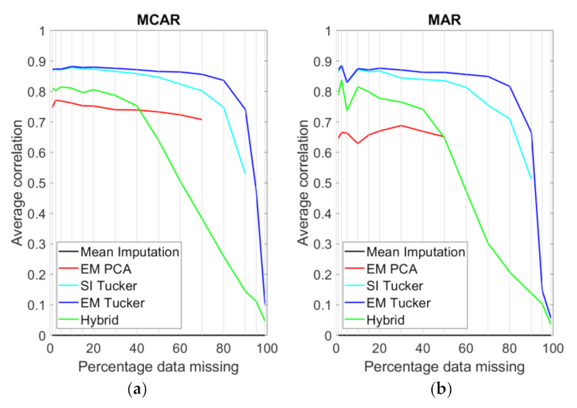
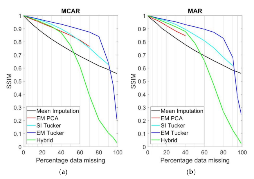
To further investigate the performance of the methods when applied to SPAIN1, the average correlation between the ground truth and the gap-filled data was calculated as shown in Equation (16) at different levels of missing data. These results are displayed in Figure 11. For the same purpose, the SSIM was calculated and is shown in Figure 12.

The SSIM and correlation analysis generally revealed the same model hierarchy as the one that was stated previously. The SSIM scores were generally higher than the correlation scores due to the fact that SSIM was calculated on a frame-by-frame basis, while the correlation was calculated on a pixel-by-pixel basis, only taking missing pixels into account. The results from the mean imputation approach had zero correlation to the original tensor. This is a model that predicted the same value ${\overline{x}}^{*}$, for every pixel that was missing, and it is therefore immediately clear that the correlation is zero. The single imputation Tucker model performed noticeably worse than EM Tucker did. EM Tucker displayed the best performance out of all of the algorithms, especially when the missing data exceeded 40%. Remarkably, EM Tucker maintained a high average correlation at very high levels of missing data. The EM Tucker reconstructions maintained the highest level of SSIM throughout all levels of missing data up to 90%, where it was outperformed by mean imputation for both MCAR and MAR. The main difference between the correlation analysis and the SSIM analysis is that EM PCA scored slightly higher on the SSIM metric in relation to the other methods.

Concluding with respect to SPAIN1, we found a clear model hierarchy in terms of gap-filling performance. EM Tucker significantly outperformed all of the methods that were tested, especially at high levels of missing data, only being outperformed by the mean imputation approach when the missing data reached 95% (for both MCAR and MAR). Single imputation Tucker generally performed better than the hybrid method, which, in turn, generally performed better than the EM PCA algorithm. The hybrid method performed slightly better in the MCAR simulated homogenous case when the frames were all equal (SIM1), but EM Tucker performed significantly better for all other cases. However, it is important to note here that the real missing data in the Iberian data set are not MCAR—they more closely resemble the MAR case.

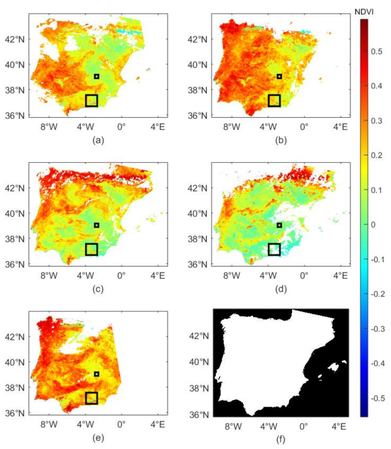
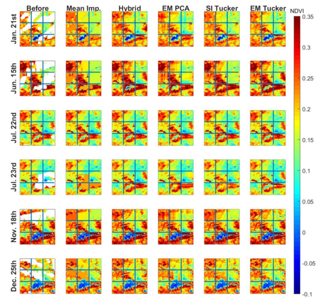
Lastly, naturally missing data from the fourth data set, namely SPAIN2, was gap-filled using the five methods. The results for the selected time frames are shown in Figure 13, where the first column shows the original frames prior to imputation. Missing values are represented in white.

The individual frames indicate a grid, which specifies the nine sub-regions, that was used to gap-fill the data in an iterative fashion as outlined in Section 3.3. The time frames that were chosen to be displayed contained different levels of missing data and were sampled throughout the year to cover all seasons, with lower NDVI values in the Sierra Nevada mountains (blue color in the lower center grid). The areas with higher NDVI during the summer correspond to forested areas in mountain ranges, and the largest seasonality in NDVI corresponds to agricultural crops showing low NDVI during the summer (water limited) and winter (temperature limited). It is noteworthy that only the values that were originally missing change in the reconstructed frames. Therefore, the reconstructed frames may look somewhat similar between the models at first glance.

It is generally clear that the mean imputation method is heavily biased, as clear homogeneous patches were used to gap-fill the missing data. EM PCA, on the other hand, results in somewhat blurry reconstructions or gap-filled information. In contrast, SI Tucker, the hybrid method, and EM Tucker lead to well-balanced imputations. Nonetheless, the gap-filled information differs for these three algorithms. 23 July clearly indicates that SI Tucker results in different reconstructions, i.e., when looking at the middle right sub-region. For the purposes of interpretation, we have included the results for the previous day, namely 22 July. Given the assumption that we would not expect regions to change drastically from one day to another, one can conclude that SI Tucker fails to predict higher NDVI regions in the middle-right sub-region of 23 July. EM Tucker as well as the hybrid method results support that conclusion, as both methods predict higher NDVIs in that region.

The computation times for all of the methods applied to SPAIN2 are shown in

Table 3. Total computation time for all methods applied to SPAIN2.

Method	Total Computation Time [s]
Simple mean imputation	0.03
Single imputation Tucker	5.11
Hybrid method	1.26
EM PCA	6.06
EM Tucker	363.94

. This is the combined time that it took to the impute missing data for all nine sub-tensors within SPAIN2. EM Tucker was noticeably slower than the other methods, with a total imputation time of just over 6 min. The analysis was conducted on an Intel(R) Core i5-8250U with 4.00 GB RAM.

5. Discussion

Looking at the results, it appears that both the hybrid method as well as EM Tucker are good choices for gap-filling missing NDVI image data. While the application of the hybrid method is easily scalable to larger geographical areas due to the simple nature of the algorithm, i.e., each pixel can be processed individually, the major advantage of EM Tucker becomes evident when large fractions of the data are missing. Our results show that EM Tucker can beat the performance of the hybrid method in such cases. This can be explained by the fact that EM Tucker utilizes temporal as well as spatial information simultaneously, while the algorithm of the hybrid method uses either one or the other to gap-fill the missing elements. In addition, we showed that EM Tucker performs better than the SI Tucker algorithm due to the fact that the former updates the imputed values during the alternating least squares fitting procedure, as seen in Equation (10). This makes the EM Tucker algorithm less prone to being negatively affected by initial incorrect imputations, i.e., the initial replacement of missing elements with column, row, or tensor means or combinations thereof.

The results obtained through the simulation studies were used to evaluate and compare the gap-filling performance of the algorithms. Furthermore, these results were utilized to define model selection strategies, i.e., to choose to correct number of components for the Tucker decomposition. We have compared methods under two scenarios, namely when data were missing completely at random (MCAR) and when data were missing at random (MAR), i.e., block-wise. Although we stated that natural missing data would match the MAR scenario, one must underline the fact that certain geographical regions, e.g., mountainous areas, might violate the randomness assumption, meaning that cloud patches might not be randomly distributed, both with respect to temporal as well as to the spatial domain. To avoid problems and to ensure that our results from SIM1, SIM2, and SPAIN1 generalize well to real-world applications, we suggest gap-filling larger areas iteratively using sub-regions of sufficiently small geographical size. This will reduce model complexity and will enable the method to be applied to very large areas, as the decompositions of the individual sub-regions can be distributed across several computational workers.

Besides the imputation of missing data, tensor decompositions such as Tucker can be used to detect anomalies if the data contain spatial or temporal indications of them. These anomalies can be caused by sudden phenological changes from, e.g., fire, insect attacks, deforestation, or drought. As discussed in Section 3.3, this would lead to additional independent temporal profiles and, therefore, could only be explained by the Tucker model if the time mode components were increased accordingly. For monitoring purposes, scores in the loading matrix A together with the abnormal residuals in $\mathcal{E}$ could be used to identify outlying behavior (see Figure 6a). However, it was not within the scope of this study to evaluate the methods towards their ability to detect anomalies or outliers. We refer the reader to other studies that highlight the potential of tensor decompositions for anomaly detection in satellite data [64].

6. Conclusions

In this study, we presented a proof-of-concept that EM Tucker can be used to gap-fill missing data in NDVI satellite images. We benchmarked the method against four reference methods using three data sets with simulated clouds as well as one real-world data set. While missing data were added artificially to the simulated data sets, a sub-region of the Iberian Peninsula was used to gap-fill naturally occurring missing data. Benchmark results indicated that EM Tucker offers superior performance in terms of reconstruction accuracy, especially when larger fractions of up to 95% of the data were missing. This could be well explained by the fact that the algorithm utilizes temporal as well as spatial information in a simultaneous fitting procedure, allowing to all of the available systematic variation to be incorporated in order to reconstruct the missing elements.

To underline the applicability of the method to real-world scenarios, we applied EM Tucker to a larger area in the south of the Iberian Peninsula, which contained 15% missing data overall. The results were presented visually and were compared to the four reference methods. In order to process larger regions, we propose dividing the area into smaller geographical sub-regions to be gap-filled individually. This approach lowers the requirements for computational resources, while offering the ability to process sub-regions in parallel at the same time. This can be understood as processing a given area using a “moving box” imputation.

The results suggest that EM Tucker is a viable method to correct measuring errors and to fill in missing data for satellite imagery. Furthermore, the high accuracy of the algorithm could enable improved satellite imagery pre-processing, especially when a big proportion of the data are corrupted or missing.