
Impacts of Spatial Configuration of Land Surface Features on Land Surface Temperature across Urban Agglomerations, China


Abstract
:1. Introduction
2. The Study Region and the Data
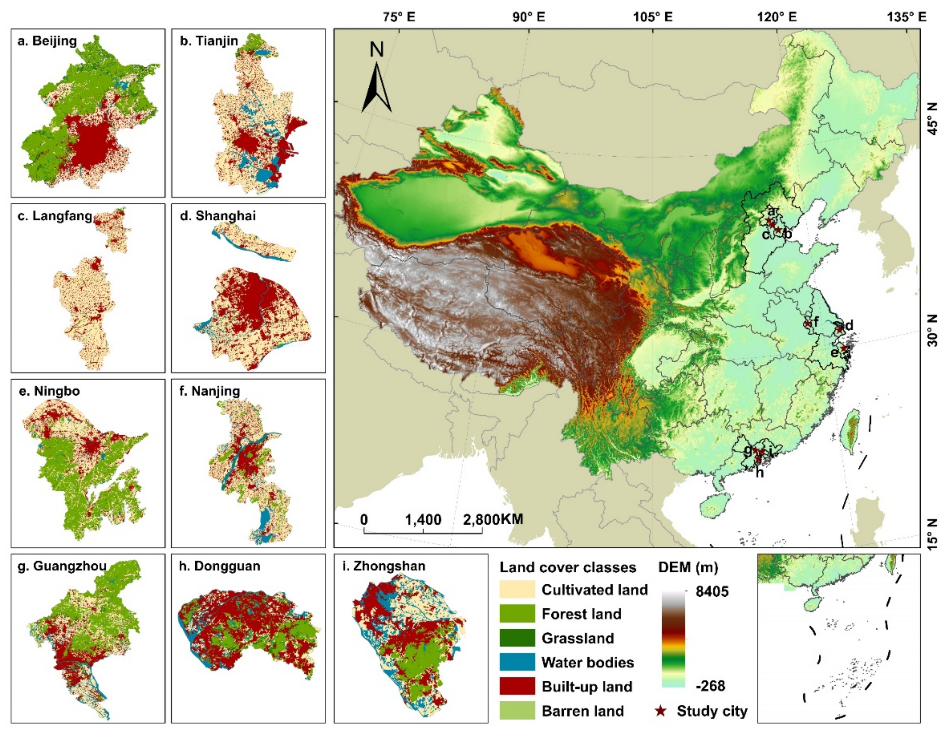
2.1. The Study Region
2.2. The Data
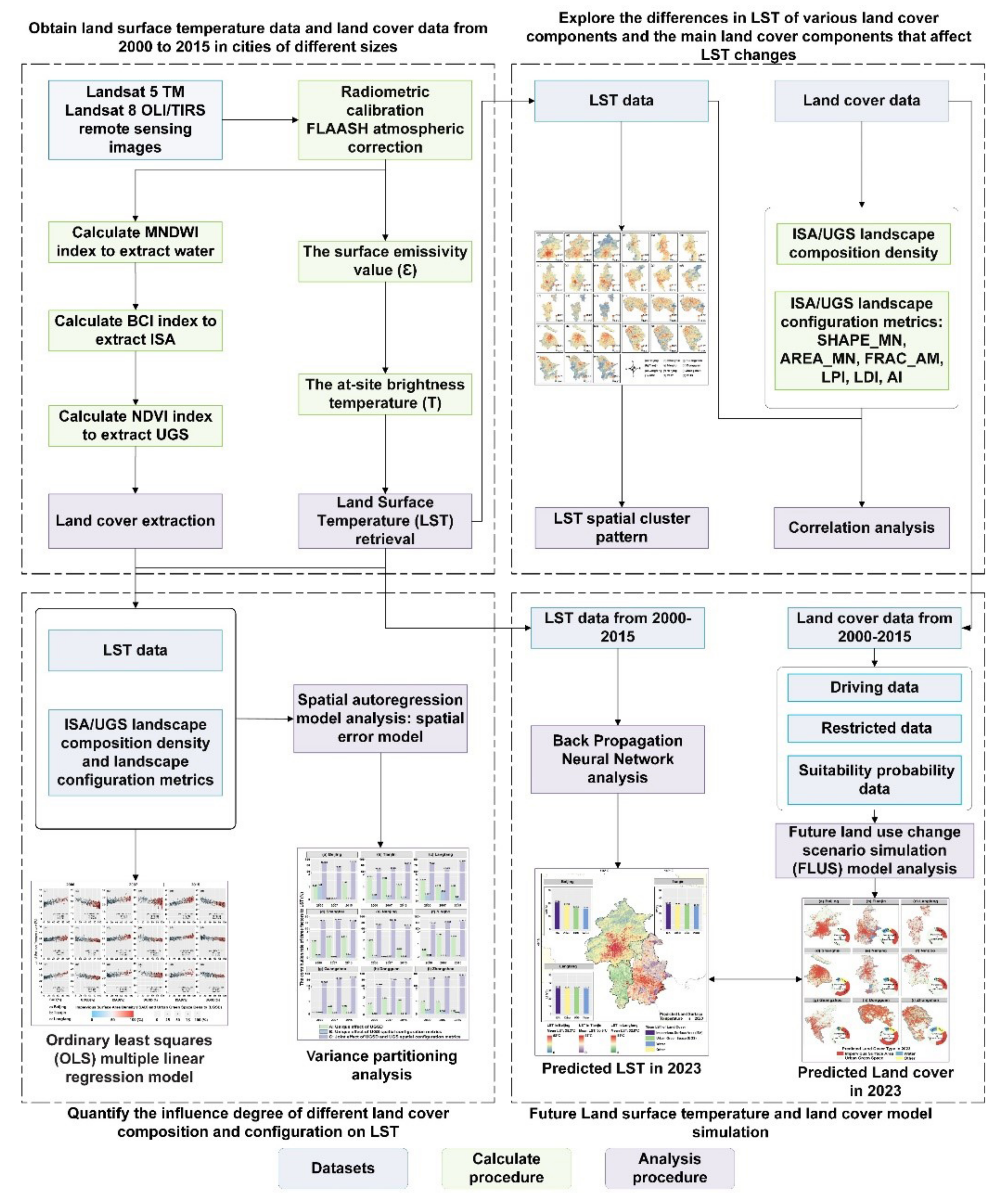
3. Methods
3.1. Land Surface Temperature (LST) Retrieval
3.2. Extraction of the Land Surface Components (LSC)
3.3. Spatial Pattern of the Land Surface Components
3.4. Pearson Correlation Analysis
3.5. Spatial Regression Model
3.6. Variance Partitioning
3.7. Modeling of Future Changes in the LSC
3.8. Prediction of the LST
4. Results and Discussion
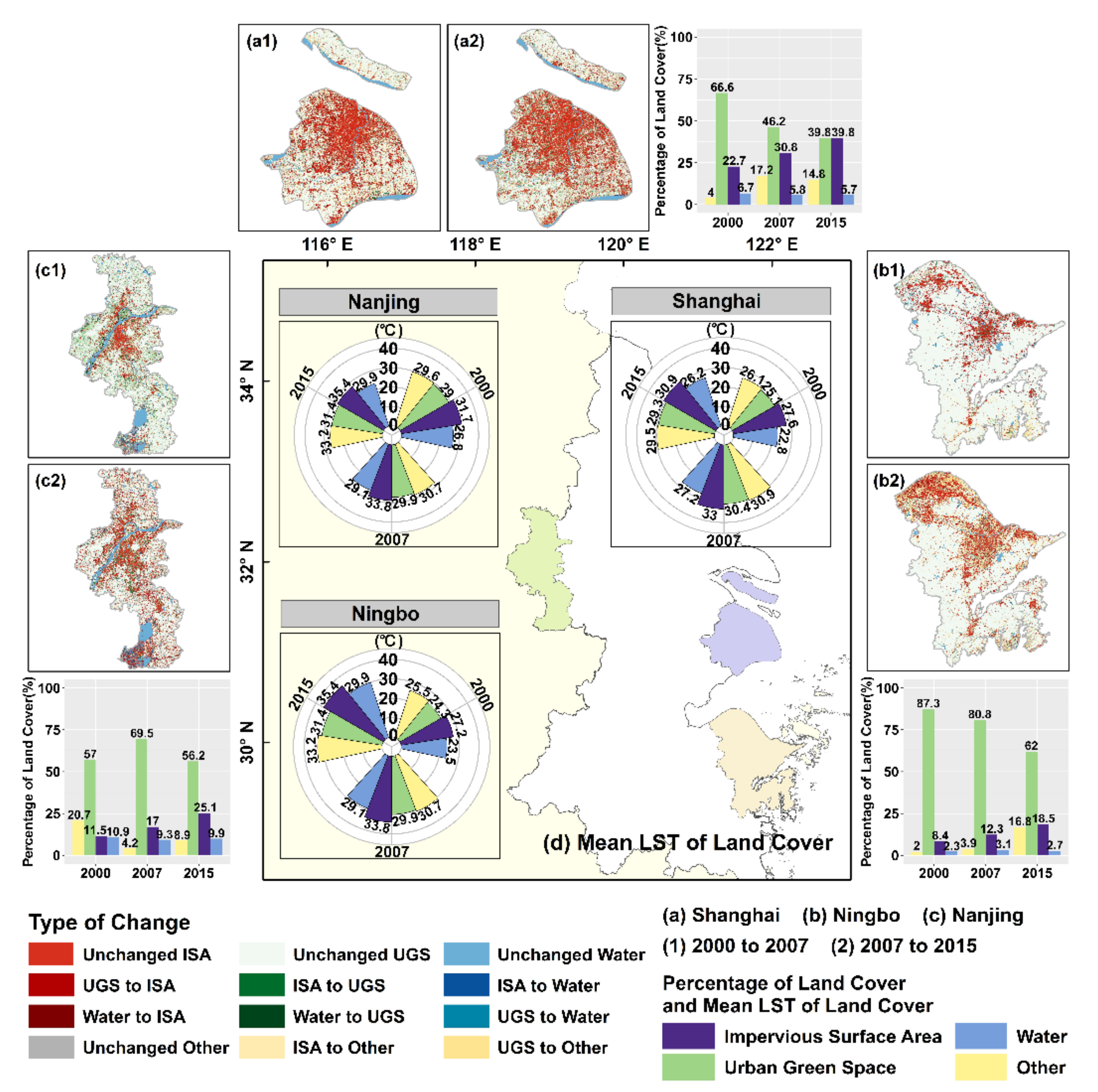
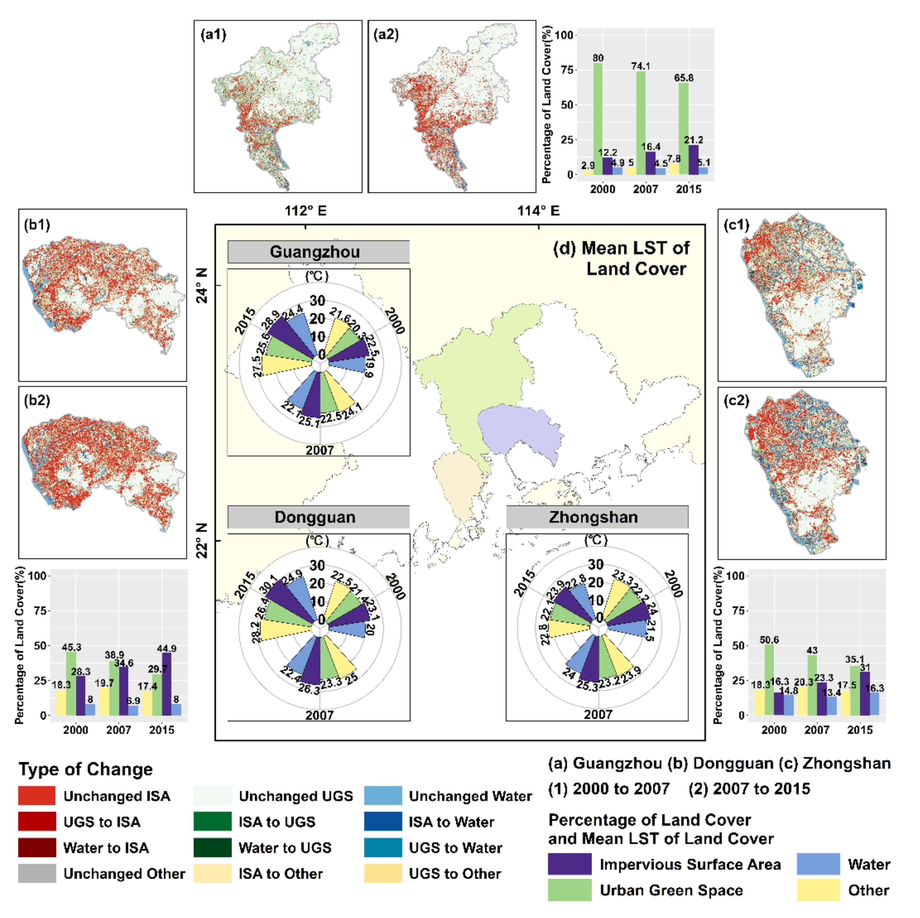
4.1. Spatial Pattern of the LST and LSC
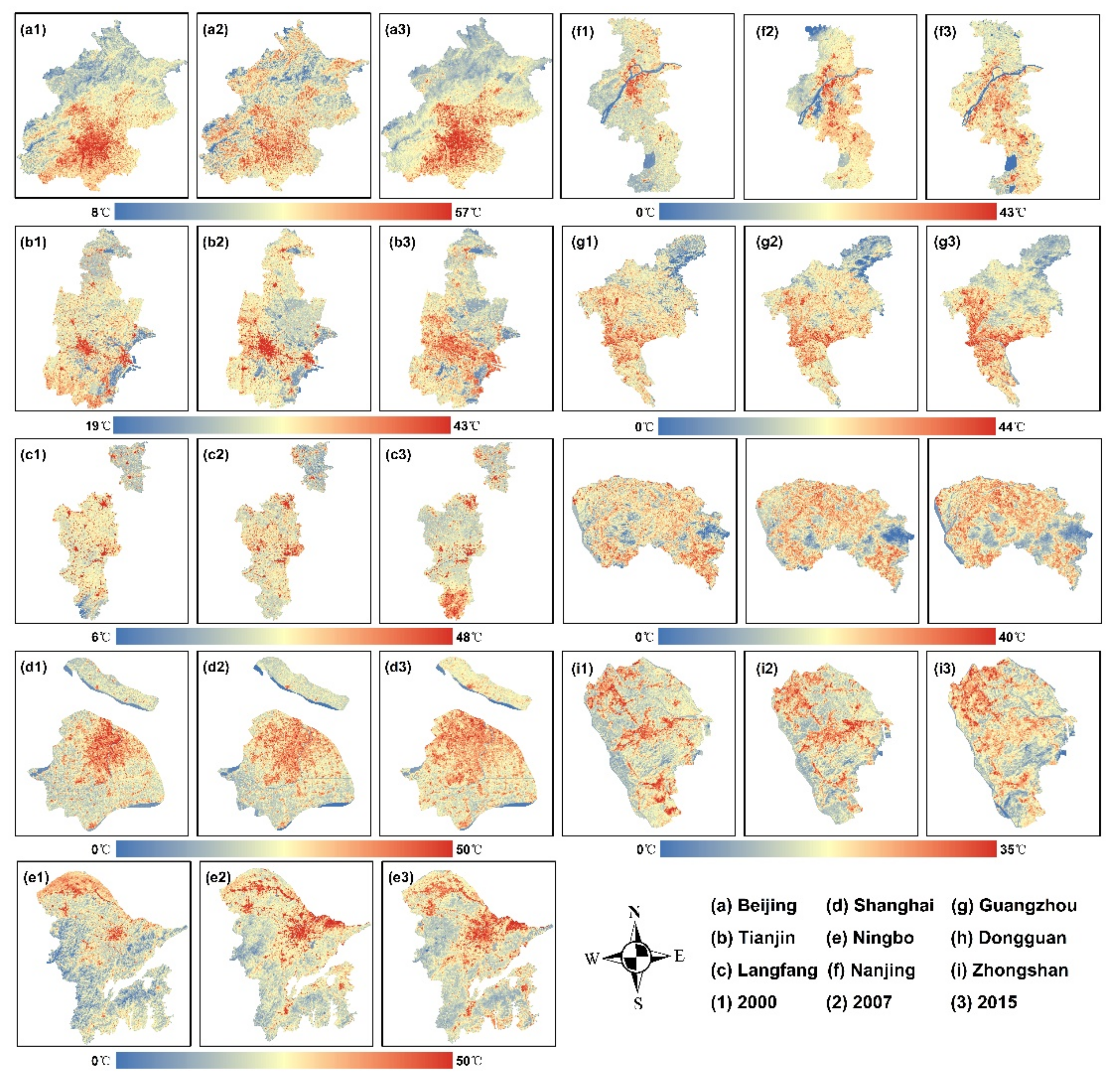
4.1.1. Changes in LST during 2000–2015
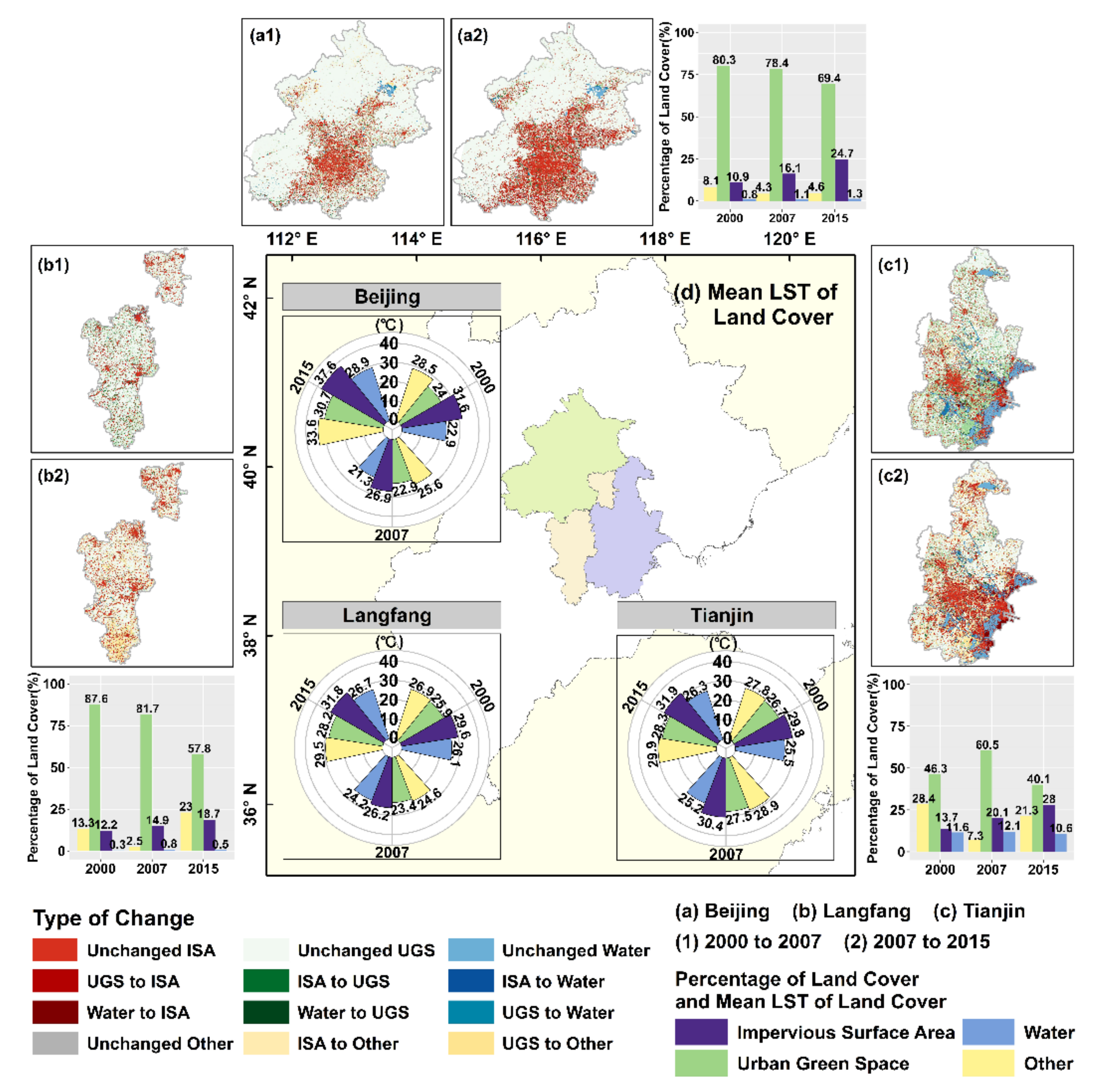
4.1.2. Changes in Spatial Pattern of the LSC during 2000–2015
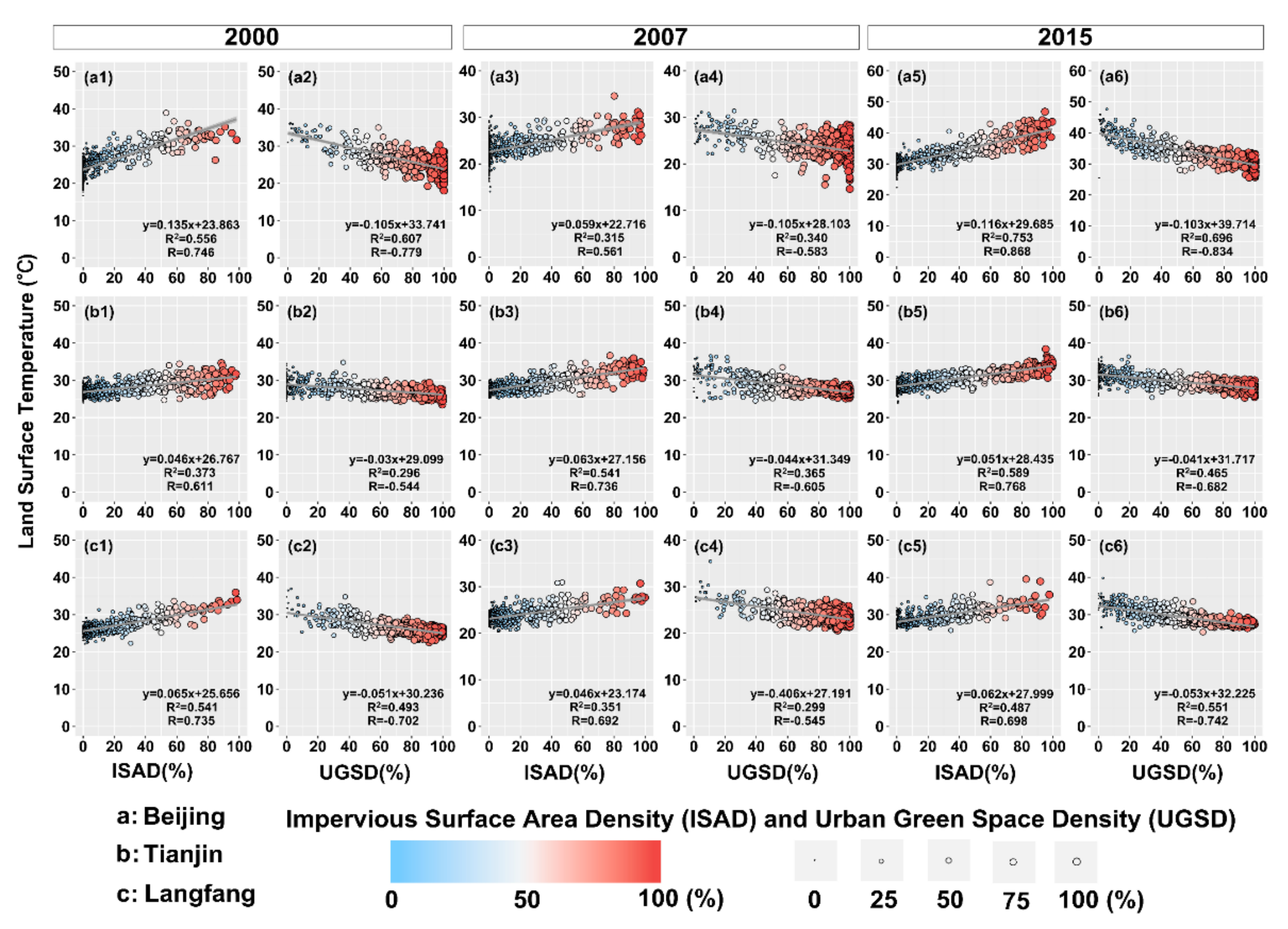
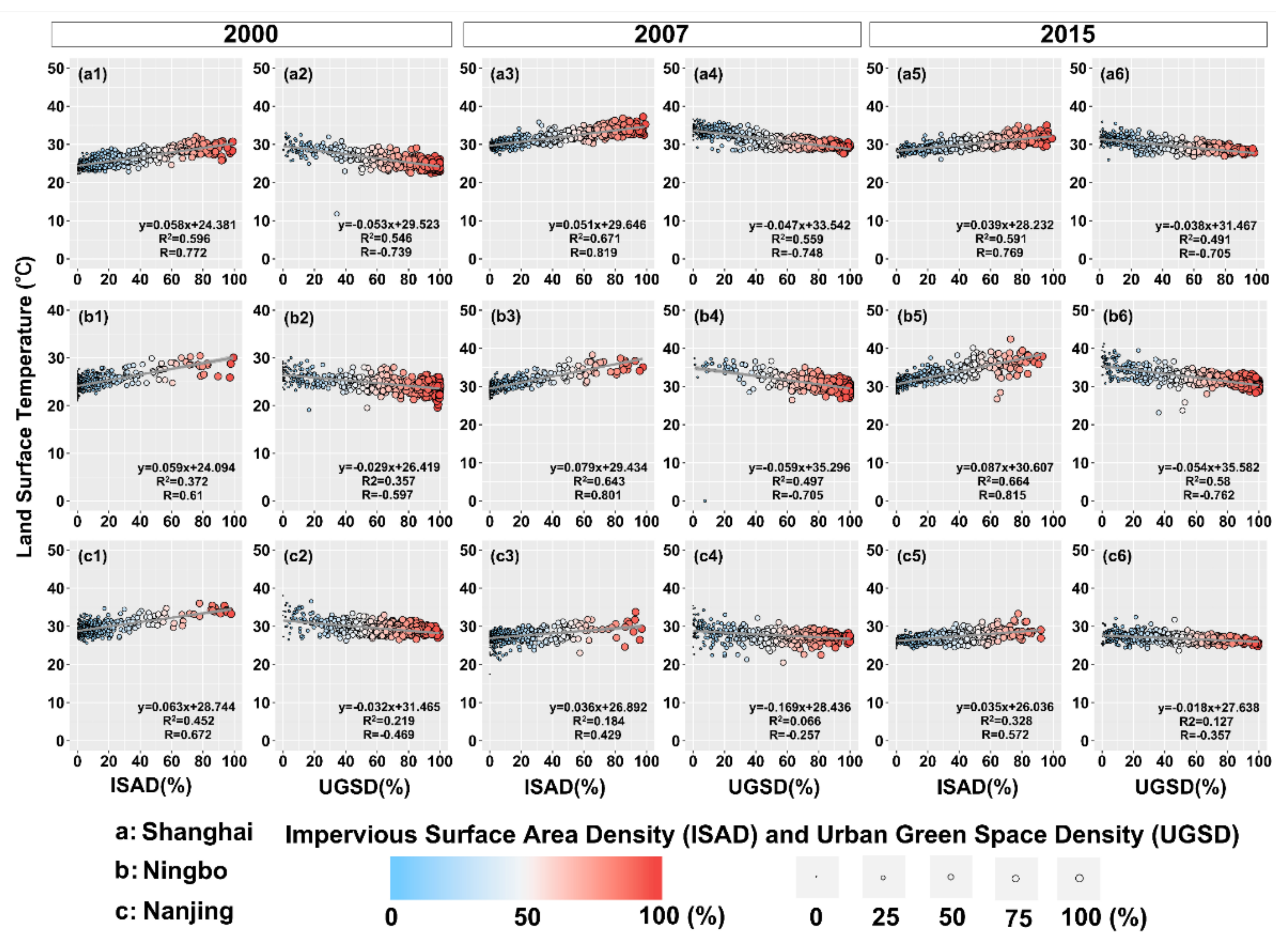
4.2. Impacts of Spatial Pattern of LSC on LST
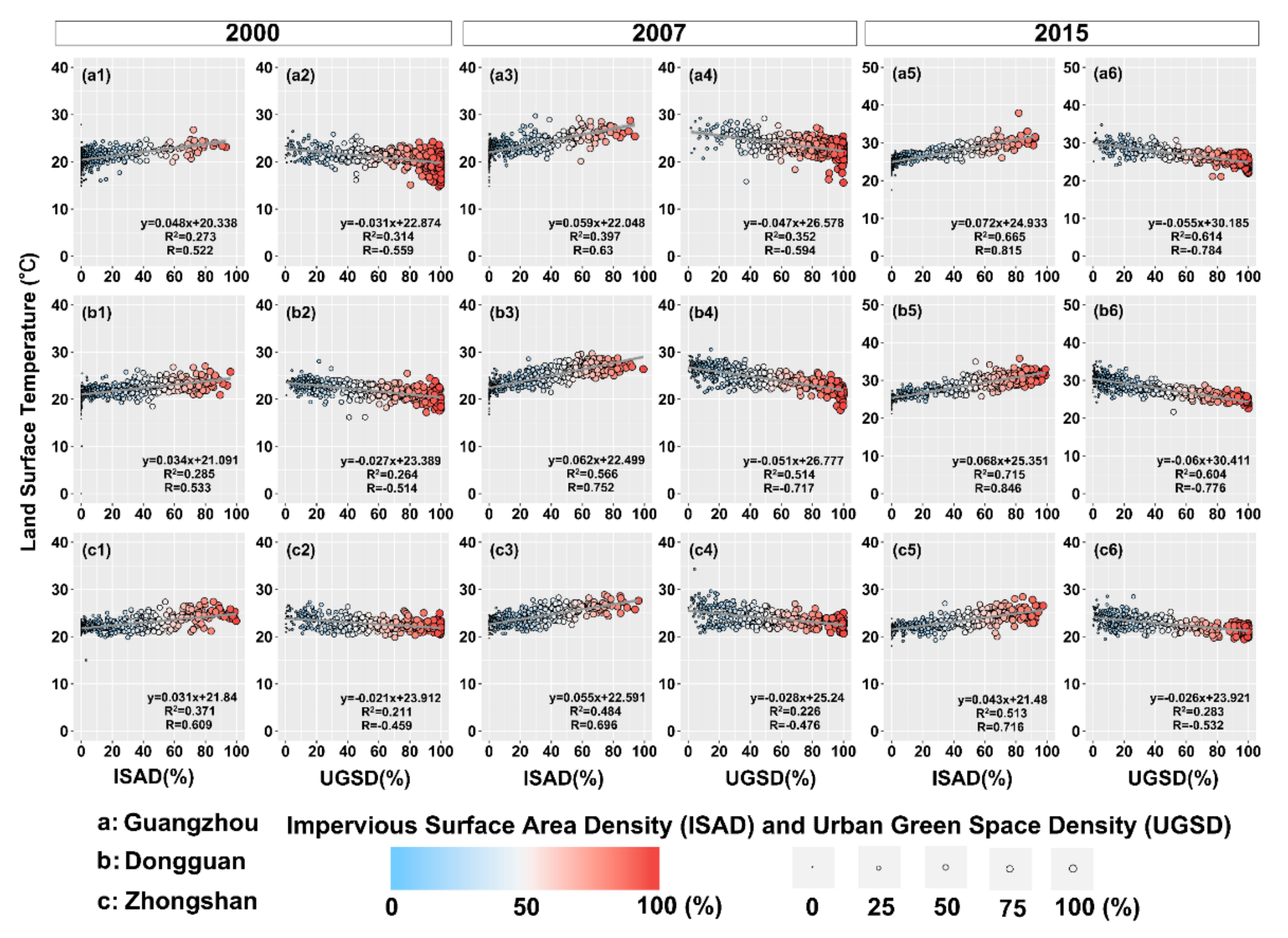
4.2.1. Relation between LSC and LST
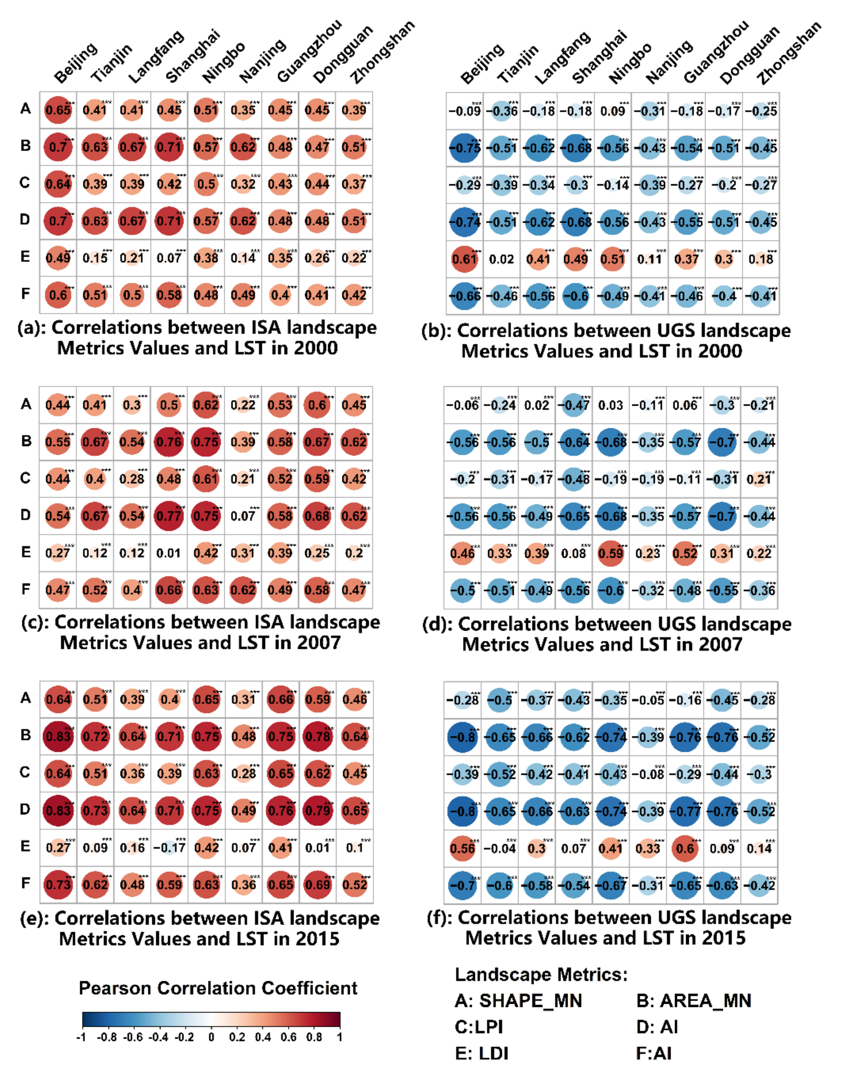
4.2.2. Relation between Spatial Configuration of LSC and LST
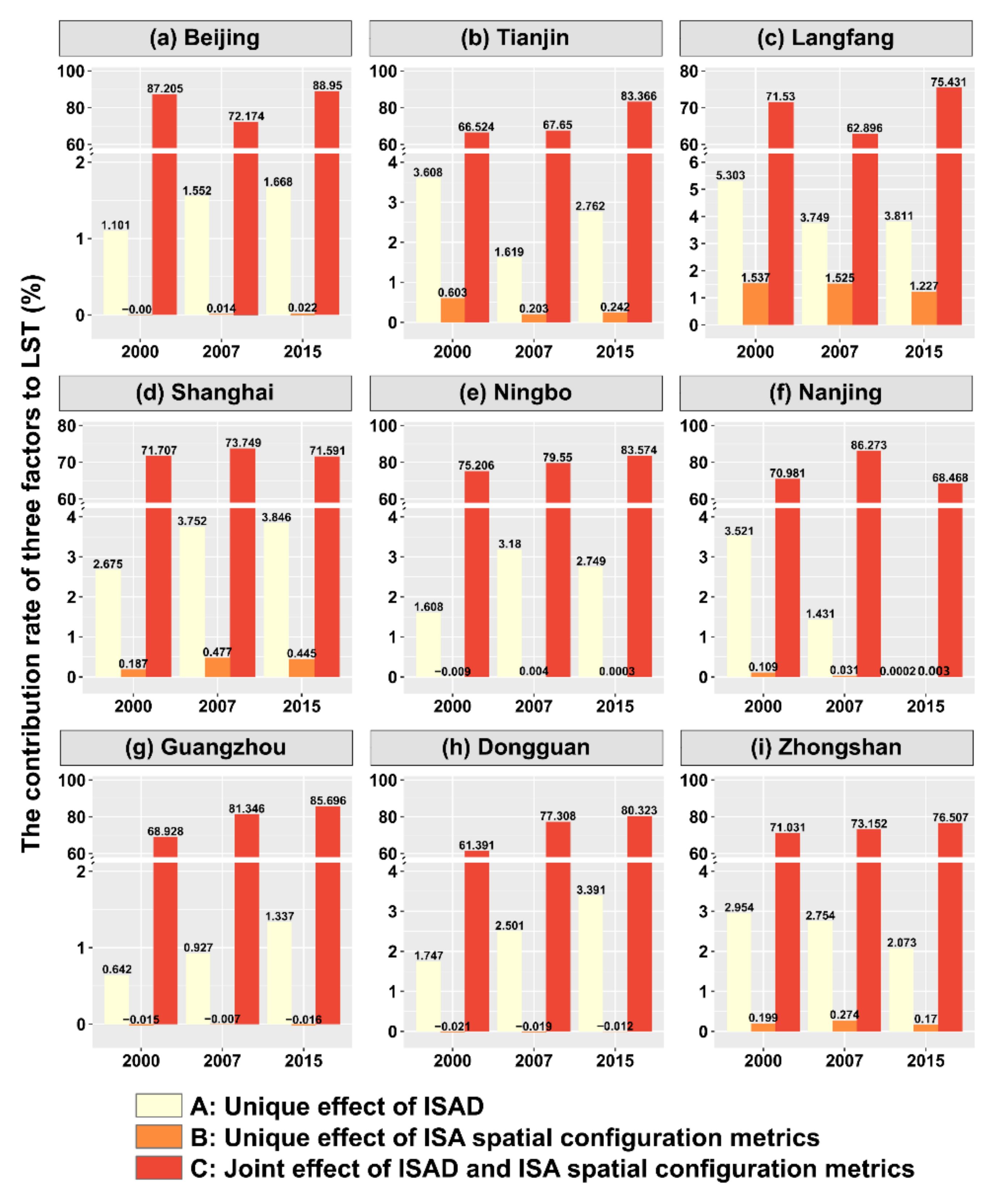
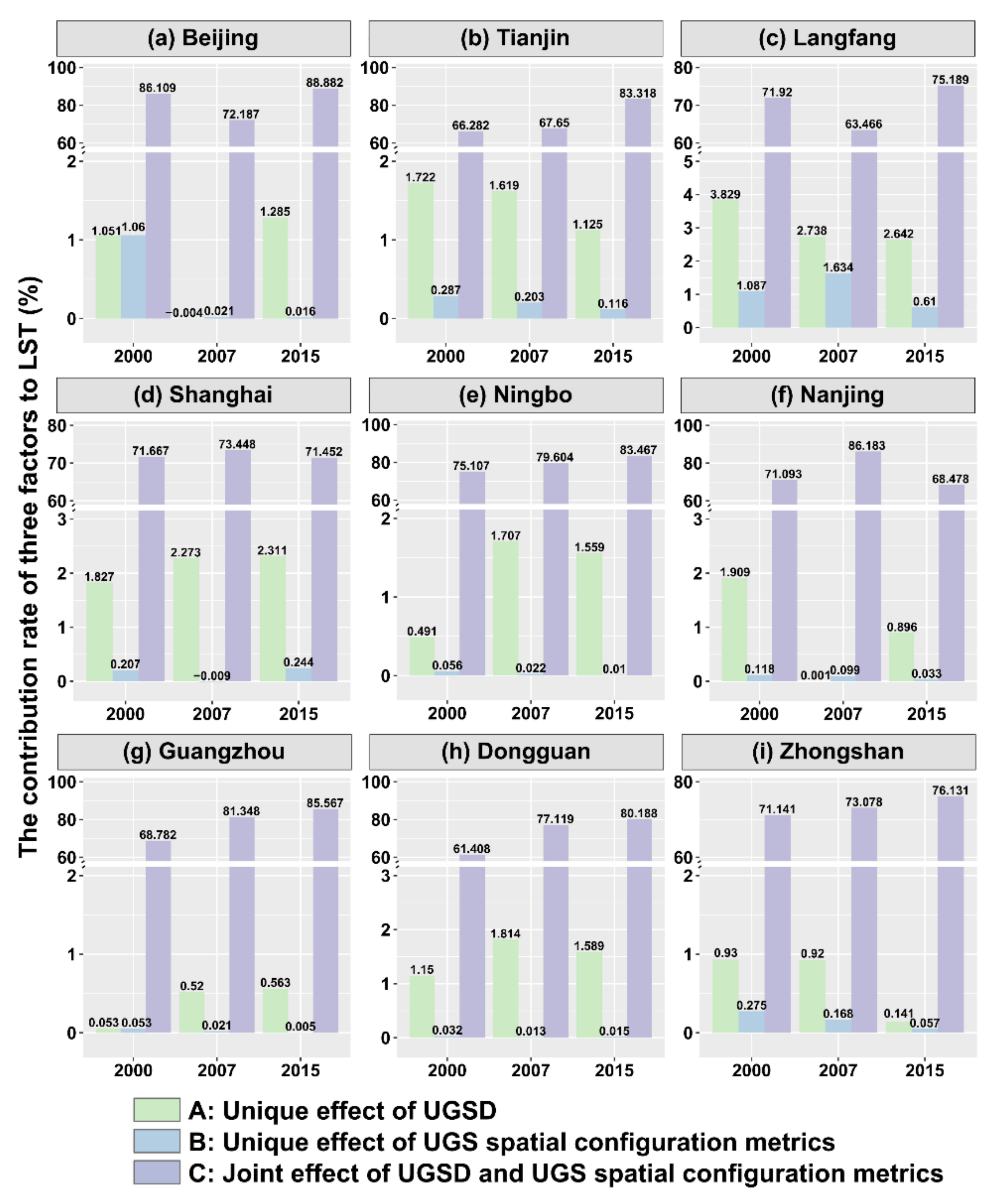
4.2.3. The Contribution of the Composition and Configuration of the LSC to LST
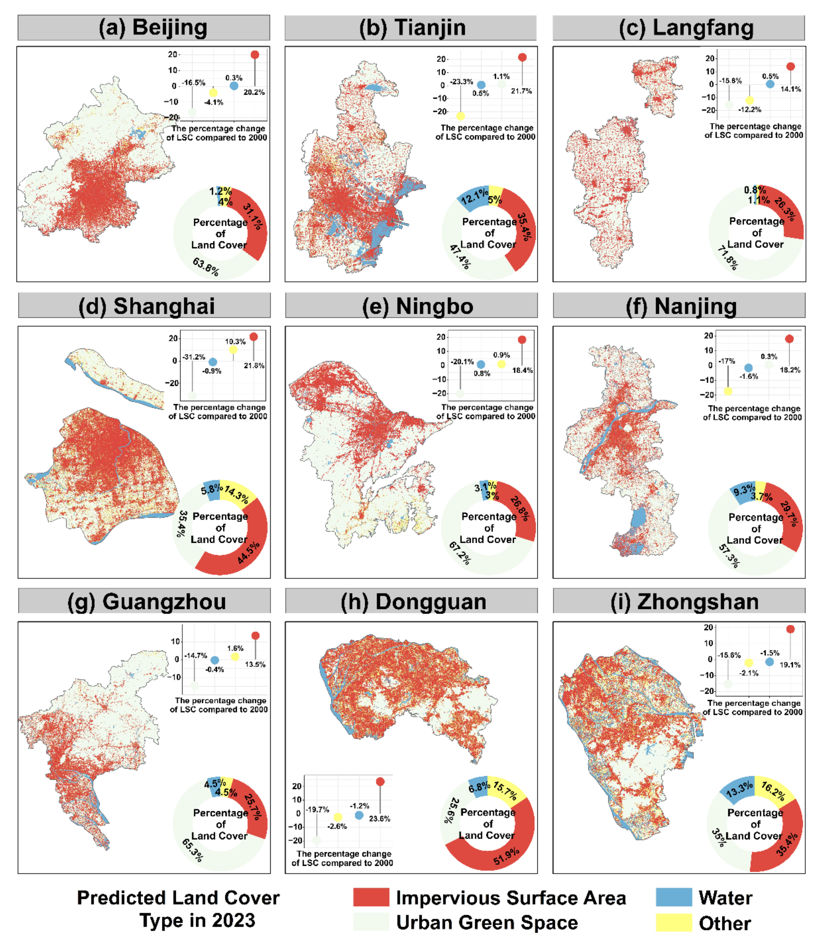
4.3. Modeling of Future LST and LSC
4.3.1. Modeling of the Future LSC
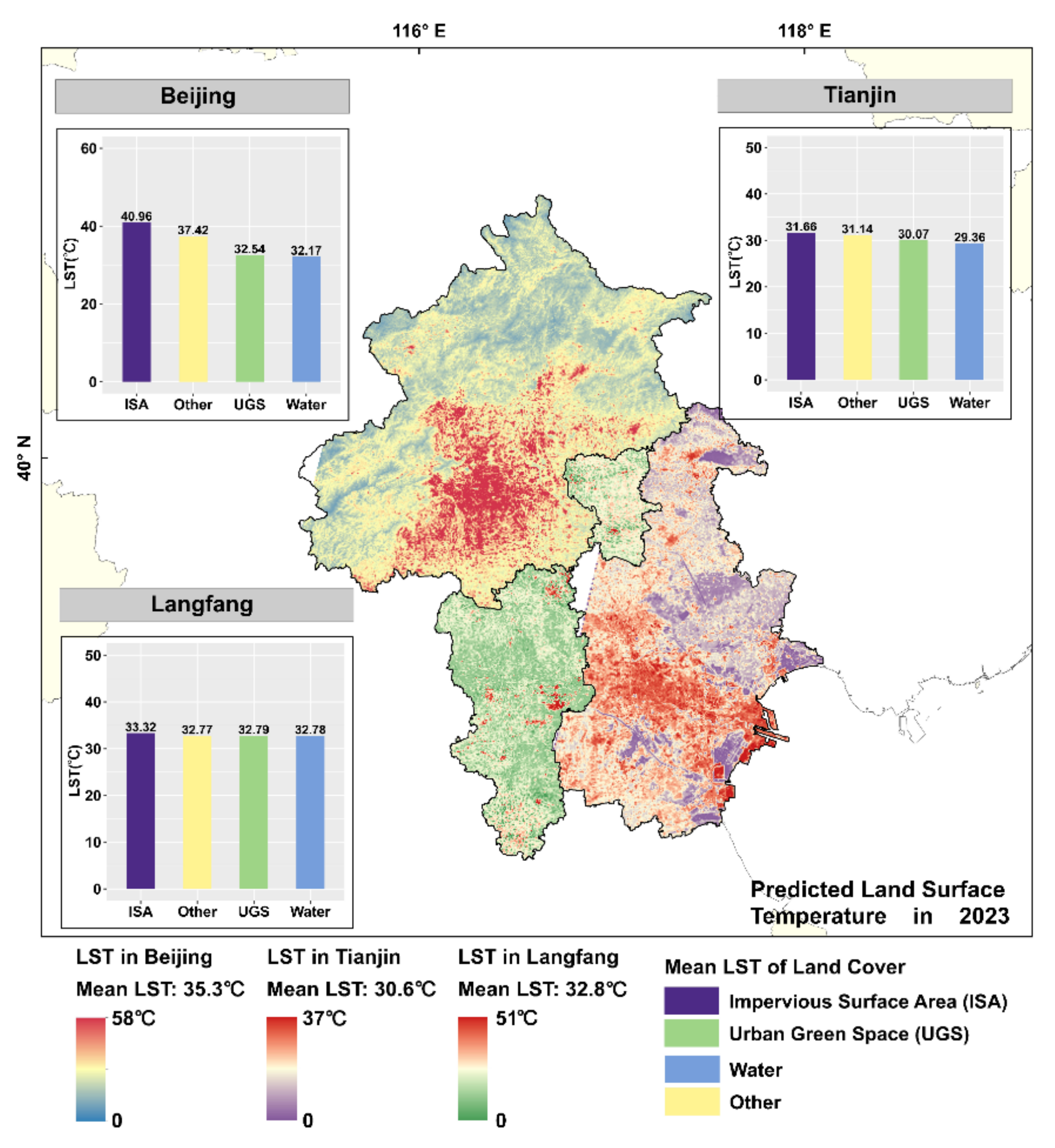
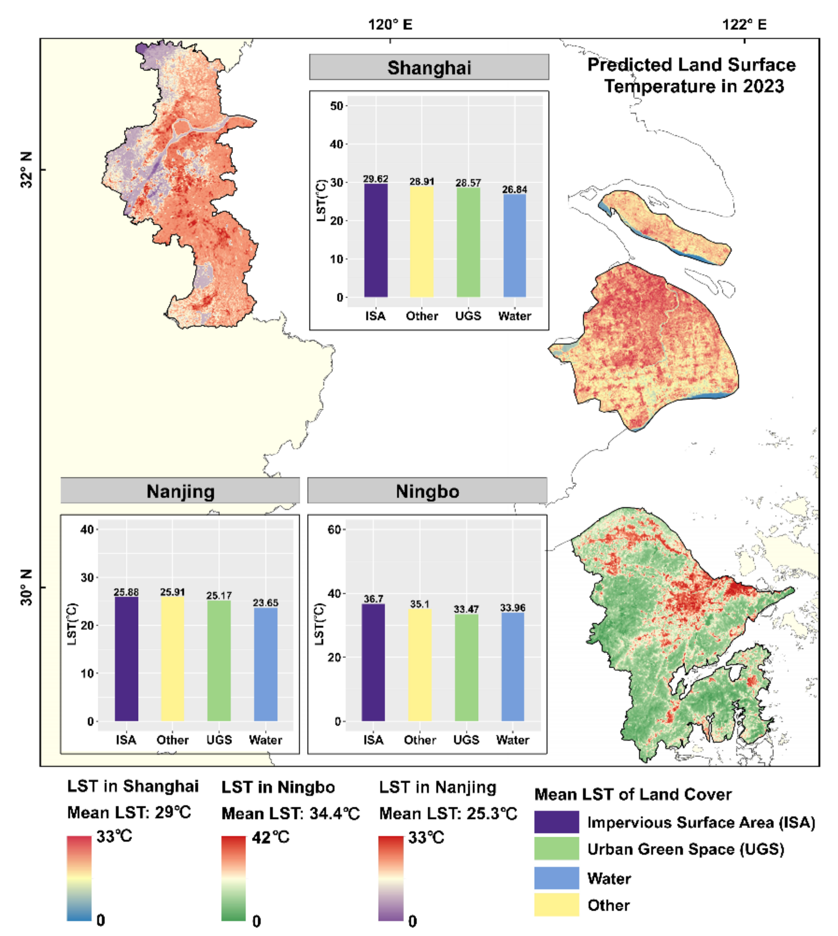
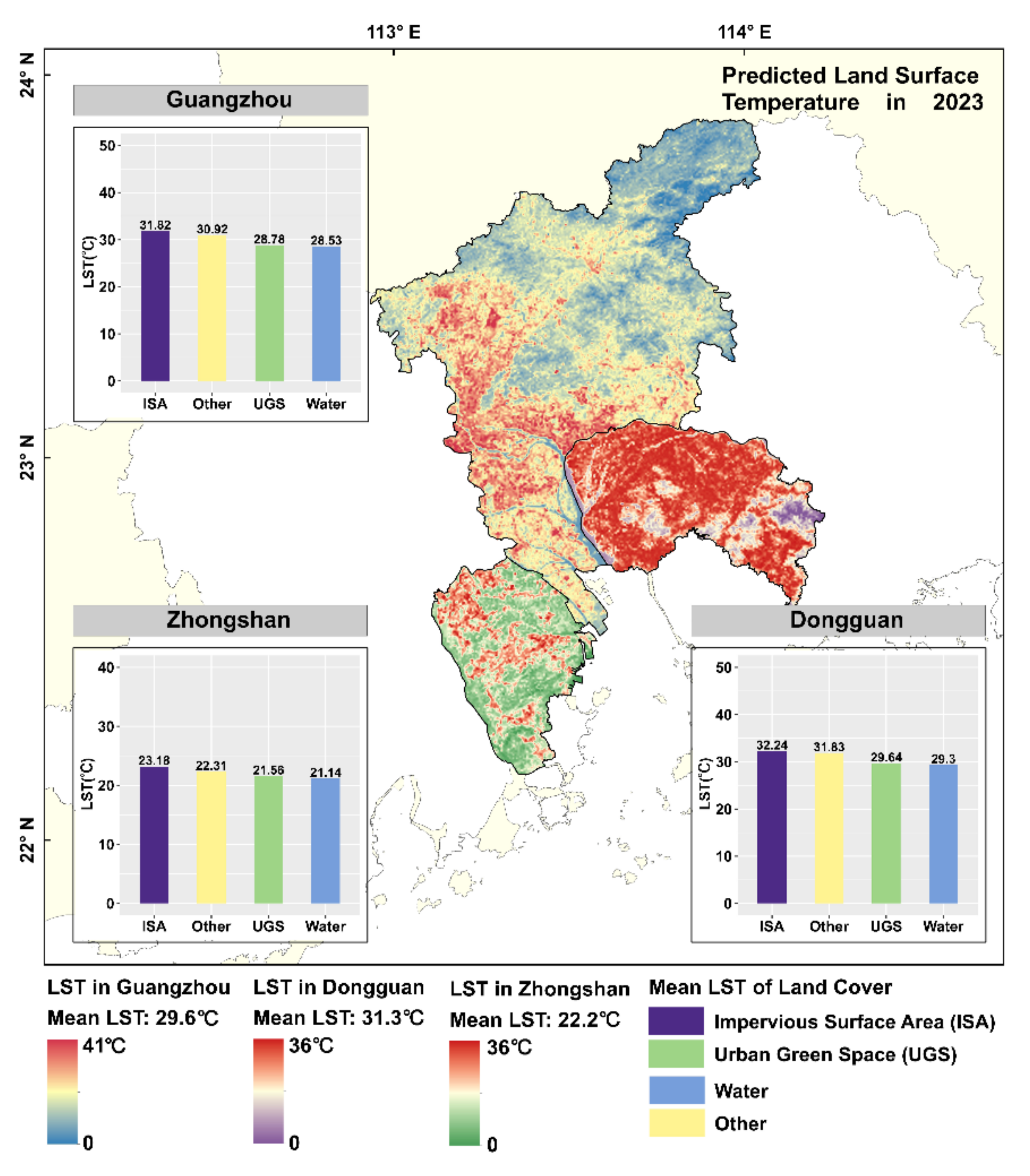
4.3.2. Modeling of Future LST Changes
5. Conclusions
Author Contributions
Funding
Institutional Review Board Statement
Informed Consent Statement
Data Availability Statement
Acknowledgments
Conflicts of Interest
Appendix A

| Landsat Satellites | Landsat Data Identification | Data Acquisition Time |
|---|---|---|
| 2000 Landsat 5 TM | LT51230322000145BJC00 | 24 May 2000 |
| LT51230332000145BJC00 | 24 May 2000 | |
| LT51220322000170BJC00 | 18 June 2000 | |
| LT51220332000170BJC00 | 18 June 2000 | |
| LT51180382000158BJC02 | 06 June 2000 | |
| LT51180392000158BJC02 | 06 June 2000 | |
| LT51180402001080BJC00 | 21 March 2001 | |
| LT51200372000140BJC00 | 19 May 2000 | |
| LT51200382000204BJC00 | 22 July 2000 | |
| LT51220432001060BJC00 | 01 March 2001 | |
| LT51220442001060BJC00 | 01 March 2001 | |
| LT51220452001060BJC00 | 01 March 2001 | |
| 2007 Landsat 5 TM | LT51230322007148IKR00 | 28 May 2007 |
| LT51230323007148IKR00 | 28 May 2007 | |
| LT51220322009258IKR00 | 15 September | |
| LT51220332009242IKR00 | 30 August 2009 | |
| LT51180382007209BJC00 | 28 July 2007 | |
| LT51180392007209BJC00 | 28 July 2007 | |
| LT51180402007209BJC00 | 28 July 2007 | |
| LT51200372006140BJC01 | 20 May 2006 | |
| LT51200382007207IKR00 | 26 July 2007 | |
| LT51220432008208BKT00 | 26 July 2008 | |
| LT51220442008208BKT00 | 26 July 2008 | |
| LT51220452009290BJC00 | 17 October 2009 | |
| 2015 Landsat 8 OLI/TIRS | LC81230322015106LGN00 | 16 April 2015 |
| LC81230332015106LGN01 | 16 April 2015 | |
| LC81220322015227LGN01 | 15 August 2015 | |
| LC81220332015275LGN00 | 02 October 2015 | |
| LC81180382015215 LGN00 | 03 August 2015 | |
| LC81180392015215LGN00 | 03 August 2015 | |
| LC81180402015215LGN00 | 03 August 2015 | |
| LC81200372016344LGN01 | 09 December 2016 | |
| LC81200382016344LGN01 | 09 December 2016 | |
| LC81220432015291LGN00 | 18 October 2015 | |
| LC81220442015291LGN01 | 18 October 2015 | |
| LC81220452015003LGN00 | 03 January 2015 |
| City | Year | ISAD | SHAPE-MN | AREA-MN | FRAC-AM | LPI | LDI | AI | R2 | Moran’I | AIC |
|---|---|---|---|---|---|---|---|---|---|---|---|
| Beijing | 2000 | 0.674 *** | 0.047 *** | 0.064 *** | −0.158 *** | −0.059 ** | 0.296 *** | 0.014 *** | 0.592 | 0.724 *** | 541094 |
| 2007 | 0.541 *** | −0.058 *** | 0.256 *** | −0.212 *** | −0.126 *** | 0.304 *** | −0.026 *** | 0.325 | 0.644 *** | 682229 | |
| 2015 | 0.788 *** | −0.095 *** | 0.077 *** | 0.707 *** | −0.349 *** | −0.413 *** | 0.03 *** | 0.759 | 0.658 *** | 393801 | |
| Tianjin | 2000 | 0.777 *** | −0.172 *** | 0.929 *** | −0.482 *** | −0.713 *** | 0.501 *** | −0.021 *** | 0.469 | 0.524 *** | 382749 |
| 2007 | 0.049 *** | −0.203 *** | 0.016 | 0.125 *** | 0.75 *** | 0.024 | −0.054 *** | 0.456 | 0.491 *** | 379852 | |
| 2015 | 0.874 *** | −0.083 *** | 0.373 *** | 0.025 | −0.444 *** | 0.089 *** | 0.001 | 0.603 | 0.68 *** | 329310 | |
| Langfang | 2000 | 0.769 *** | −0.294 *** | 1.138 *** | −0.578 *** | −0.777 *** | 0.642 *** | −0.094 *** | 0.551 | 0.579 *** | 226556 |
| 2007 | 0.593 *** | −0.403 *** | 1.44 *** | −1.275 *** | −0.689 *** | 1.296 *** | −0.161 *** | 0.366 | 0.56 *** | 264969 | |
| 2015 | 0.686 *** | −0.222 *** | 0.996 *** | −0.891 *** | −0.453 *** | 0.835 *** | −0.101 *** | 0.497 | 0.658 *** | 239078 | |
| Shanghai | 2000 | 0.823 *** | −0.015 | 0.34 *** | −0.93 *** | 0.128 *** | 0.782 *** | −0.042 *** | 0.607 | 0.437 *** | 192958 |
| 2007 | 0.909 *** | −0.093 *** | 0.791 *** | −0.884 *** | −0.216 *** | 0.798 *** | −0.057 *** | 0.69 | 0.391 *** | 168755 | |
| 2015 | 0.814 *** | −0.098 *** | 0.684 *** | −0.326 *** | −0.362 *** | 0.355 *** | −0.039 *** | 0.61 | 0.47 *** | 191986 | |
| Ningbo | 2000 | 0.605 *** | 0.015 | 0.132 *** | −0.164 *** | −0.169 *** | 0.307 *** | 0.018 ** | 0.405 | 0.645 *** | 318874 |
| 2007 | 0.816 *** | 0.037 ** | 0.067 * | −0.068 | −0.13 *** | 0.154 *** | 0.011 * | 0.667 | 0.549 *** | 235489 | |
| 2015 | 0.789 *** | 0.014 | 0.149 *** | −0.174 *** | −0.105 *** | 0.239 *** | 0.009** | 0.684 | 0.617 *** | 229122 | |
| Nanjing | 2000 | 0.722 *** | −0.107 *** | 0.421 *** | −0.828 *** | −0.107 * | 0.764 *** | −0.046 *** | 0.471 | 0.588 *** | 215496 |
| 2007 | 0.48 *** | −0.24 *** | 0.469 *** | 0.184 * | −0.469 *** | 0.0189 | −0.009 | 0.194 | 0.863 *** | 264010 | |
| 2015 | 0.014 *** | −0.109 *** | −0.371 *** | 0.0403 | 0.911 *** | 0.053 | −0.052 *** | 0.218 | 0.612 *** | 257677 | |
| Guangzhou | 2000 | 0.481 *** | 0.074 *** | −0.028 | −0.438 *** | 0.11** | 0.449 *** | 0.003 | 0.296 | 0.599 *** | 284862 |
| 2007 | 0.592 *** | −0.011 | 0.145 *** | −0.328 *** | −0.021 | 0.433 *** | 0.026 *** | 0.427 | 0.708 *** | 265101 | |
| 2015 | 0.774 *** | 0.001 | 0.05* | −0.048 | −0.036 | 0.183 *** | 0.004 | 0.696 | 0.6 *** | 189168 | |
| Dongguan | 2000 | 0.472 *** | 0.051 * | −0.092 | −0.358 *** | 0.29 *** | 0.388 *** | −0.011 | 0.314 | 0.515 *** | 92150.1 |
| 2007 | 0.677 *** | 0.018 | −0.099 ** | −0.018 | 0.169 *** | 0.153 *** | −0.002 | 0.601 | 0.543 *** | 73249.3 | |
| 2015 | 0.799 *** | −0.021 | −0.001 | 0.121 *** | −0.007 | −0.02 | −0.000001 | 0.741 | 0.439 *** | 55702.8 | |
| Zhongshan | 2000 | 0.692 *** | −0.192 *** | 0.551 *** | −0.854 *** | −0.095 | 0.716 *** | −0.083 *** | 0.393 | 0.606 *** | 59497.9 |
| 2007 | 0.719 *** | −0.061 * | 0.413 *** | −1.179 *** | 0.171 ** | 0.987 *** | −0.092 *** | 0.499 | 0.575 *** | 55615.7 | |
| 2015 | 0.759 *** | −0.125 *** | 0.351 *** | −0.412 *** | −0.025 | 0.447 *** | −0.064 *** | 0.529 | 0.585 *** | 52061.1 |
| City | Year | UGSD | SHAPE-MN | AREA-MN | FRAC-AM | LPI | LDI | AI | R2 | Moran’I | AIC |
|---|---|---|---|---|---|---|---|---|---|---|---|
| Beijing | 2000 | −0.67 *** | 0.018 *** | 0.141 *** | −0.329 *** | 0.381 *** | 0.567 *** | −0.067 *** | 0.623 | 0.717 *** | 519350 |
| 2007 | −0.017 *** | −0.072 *** | 0.299 *** | −0.215 *** | −0.501 *** | 0.286 *** | −0.036 *** | 0.297 | 0.629 *** | 693643 | |
| 2015 | −0.784 *** | −0.033 *** | 0.241 *** | −0.024 *** | −0.222 *** | 0.029 * | 0.042 *** | 0.707 | 0.703 *** | 448522 | |
| Tianjin | 2000 | −0.586 *** | 0.175 *** | −0.867 *** | 0.159 *** | 0.562 *** | −0.305 *** | 0.055 *** | 0.338 | 0.578 *** | 421253 |
| 2007 | −0.643 *** | 0.011 * | −0.5 *** | 0.376 *** | −0.044 | −0.541 *** | −0.004 | 0.421 | 0.563 *** | 390533 | |
| 2015 | −0.695 *** | 0.092 *** | −0.521 *** | 0.087 *** | 0.363 *** | −0.22 *** | −0.0007 | 0.514 | 0.697 *** | 364348 | |
| Langfang | 2000 | −0.72 *** | 0.039 *** | −0.699 *** | 0.289 *** | −0.061 *** | −0.83 *** | −0.004 *** | 0.532 | 0.568 *** | 231241 |
| 2007 | −0.749 *** | −0.082 *** | 0.203 *** | 0.303 *** | −0.393 *** | −0.275 *** | 0.031 *** | 0.582 | 0.497 *** | 199182 | |
| 2015 | −0.75 *** | −0.033 *** | −0.425 *** | 0.479 *** | −0.241 *** | −0.734 *** | 0.007 | 0.584 | 0.53 *** | 218060 | |
| Shanghai | 2000 | −0.745 *** | 0.078 *** | −0.644 *** | 0.28 *** | 0.122 *** | −0.478 *** | 0.03 *** | 0.562 | 0.478 *** | 203939 |
| 2007 | 0.909 *** | −0.093 *** | 0.791 *** | −0.884 *** | −0.216 *** | 0.798 *** | −0.057 *** | 0.69 | 0.391 *** | 168755 | |
| 2015 | −0.767 *** | −0.073 *** | −0.232 *** | 0.688 *** | −0.191 *** | −0.633 *** | −0.016 ** | 0.523 | 0.527 *** | 212543 | |
| Ningbo | 2000 | −0.444 *** | 0.026 *** | 0.109 *** | 0.002 | −0.394 *** | −0.073* | −0.045 *** | 0.412 | 0.625 *** | 317177 |
| 2007 | −0.715 *** | 0.015 *** | −0.005 | −0.092 *** | 0.241 *** | 0.204 *** | −0.065 *** | 0.54 | 0.649 *** | 279376 | |
| 2015 | −0.809 *** | 0.004 | −0.072 * | −0.355 *** | 0.563 *** | 0.355 *** | −0.063 *** | 0.605 | 0.66 *** | 259549 | |
| Nanjing | 2000 | −0.5 *** | −0.009 | −0.199 *** | 0.014 | 0.079 * | −0.253 *** | −0.067 *** | 0.304 | 0.651 *** | 242417 |
| 2007 | 0.002 | 0.027 *** | −0.037 | 0.17 *** | −0.746 *** | −0.445 *** | 0.022 ** | 0.123 | 0.849 *** | 272507 | |
| 2015 | −0.303 *** | 0.013 | −0.115 *** | 0.332 *** | −0.517 *** | −0.45 *** | 0.042 *** | 0.178 | 0.659 *** | 262691 | |
| Guangzhou | 2000 | −0.437 *** | 0.033 *** | 0.245 *** | −0.676 *** | 0.535 *** | 0.824 *** | −0.094 *** | 0.349 | 0.568 *** | 275906 |
| 2007 | −0.542 *** | 0.039 *** | −0.032 | −0.168 *** | 0.366 *** | 0.374 *** | −0.048 *** | 0.381 | 0.73 *** | 274000 | |
| 2015 | −0.728 *** | 0.037 *** | −0.02 | −0.313 *** | 0.436 *** | 0.445 *** | −0.046 *** | 0.653 | 0.632 *** | 204422 | |
| Dongguan | 2000 | −0.453 *** | −0.0002 | 0.259 *** | −0.494 *** | 0.237 *** | 0.589 *** | −0.079 *** | 0.311 | 0.514 *** | 92337.4 |
| 2007 | −0.687 *** | −0.103 *** | 0.417 *** | −0.767 *** | 0.374 *** | 0.865 *** | −0.115 *** | 0.567 | 0.564 *** | 76395.8 | |
| 2015 | −0.786 *** | −0.044* | 0.243 *** | −0.354 *** | 0.035 | 0.293 *** | −0.044 *** | 0.651 | 0.524 *** | 66765.5 | |
| Zhongshan | 2000 | −0.501 *** | 0.013 | −0.976 *** | 0.607 *** | 0.291 ** | −0.73 *** | 0.007 | 0.24 | 0.657 *** | 65224 |
| 2007 | −0.605 *** | −0.135 *** | −0.392 *** | 0.221 ** | 0.439 *** | −0.16 ** | −0.072 *** | 0.246 | 0.678 *** | 66221 | |
| 2015 | −0.54 *** | −0.043* | −0.35 *** | −0.416 *** | 0.754 *** | 0.366 *** | −0.072 *** | 0.302 | 0.669 *** | 61937.3 |
| City | Year | ISAD | SHAPE-MN | AREA-MN | FRAC-AM | LPI | LDI | AI | R2 | AIC |
|---|---|---|---|---|---|---|---|---|---|---|
| Beijing | 2000 | 0.708 *** | 0.017 * | 0.007 | −0.144 *** | 0.023 * | 0.126 *** | 0.02 *** | 0.883 | 258028 |
| 2007 | 0.688 *** | 0.011 | 0.051 ** | −0.177 *** | −0.029 | 0.14 *** | 0.023 *** | 0.737 | 473592 | |
| 2015 | 0.863 *** | −0.068 *** | 0.096 *** | 0.088 *** | −0.095 *** | −0.025 * | 0.018 *** | 0.906 | 183419 | |
| Tianjin | 2000 | 0.953 *** | −0.122 *** | 0.964 *** | −1.043 *** | −0.601 *** | 0.899 *** | −0.069 *** | 0.707 | 302773 |
| 2007 | 0.008 *** | −0.321* | 0.555 *** | −0.608 *** | 0.522 *** | 0.666 *** | −0.101 *** | 0.682 | 309919 | |
| 2015 | 1.074 *** | −0.052 *** | 0.482 *** | −0.336 *** | −0.446 *** | 0.296 *** | −0.026 *** | 0.864 | 181627 | |
| Langfang | 2000 | 1.066 *** | −0.281 *** | 1.241 *** | −1.65 *** | −0.716 *** | 1.521 *** | −0.167 *** | 0.784 | 163139 |
| 2007 | 0.876 *** | −0.316 *** | 1.339 *** | −1.95 *** | −0.588 *** | 1.789 *** | −0.183 *** | 0.682 | 205517 | |
| 2015 | 0.951 ** | −0.192 *** | 1.08 *** | −1.554 *** | −0.495 *** | 1.368 *** | −0.144 *** | 0.805 | 155246 | |
| Shanghai | 2000 | 0.889 *** | 0.014 | 0.374 *** | −0.664 *** | −0.129 *** | 0.538 *** | −0.028 *** | 0.746 | 159735 |
| 2007 | 1.011 *** | −0.075 *** | 0.723 *** | −0.814 *** | −0.278 *** | 0.717 *** | −0.059 *** | 0.78 | 142922 | |
| 2015 | 0.952 *** | −0.059 *** | 0.589 *** | −0.476 *** | −0.271 *** | 0.462 *** | −0.041 ** | 0.759 | 154920 | |
| Ningbo | 2000 | 0.682 *** | 0.08 *** | −0.061 ** | −0.035 | −0.037 | 0.016 | 0.029 *** | 0.768 | 215893 |
| 2007 | 0.888 *** | 0.036** | −0.037 | −0.074 | −0.031 | 0.073 * | 0.026 *** | 0.827 | 166308 | |
| 2015 | 0.886 *** | 0.016 | 0.007 | −0.127 *** | 0.003 | 0.113 *** | 0.019 *** | 0.863 | 139198 | |
| Nanjing | 2000 | 0.873 *** | 0.012 | 0.271 *** | −0.651 *** | 0.079 * | −0.253 *** | −0.067 *** | 0.746 | 158792 |
| 2007 | 0.695 *** | 0.028* | 0.157 *** | −0.257 *** | −0.095 *** | 0.227** | −0.009 | 0.877 | 102932 | |
| 2015 | 0.003 * | −0.103 *** | 0.114 *** | −0.258 *** | 0.326 *** | 0.275 *** | −0.034 *** | 0.685 | 187073 | |
| Guangzhou | 2000 | 0.465 *** | 0.059 *** | −0.026 | −0.146 * | 0.043 | 0.112 | 0.011* | 0.696 | 209781 |
| 2007 | 0.612 *** | 0.024 * | 0.03 | −0.14 ** | −0.008 | 0.118 ** | 0.004 | 0.823 | 154786 | |
| 2015 | 0.795 *** | 0.032 *** | −0.019 | −0.082** | 0.012 | 0.071 ** | 0.013 *** | 0.87 | 112694 | |
| Dongguan | 2000 | 0.537 *** | 0.063** | −0.075 * | −0.12 | 0.103 * | 0.093 | 0.007 | 0.631 | 74375.7 |
| 2007 | 0.73 *** | 0.015 | −0.095 *** | 0.028 | 0.085 * | 0.009 | 0.007 | 0.798 | 53227.4 | |
| 2015 | 0.865 *** | 0.004 | −0.041 | −0.0007 | −0.003 | 0.007 | −0.044 *** | 0.837 | 42713.4 | |
| Zhongshan | 2000 | 0.249 *** | −0.077 ** | 0.619 *** | −0.795 *** | −0.269 ** | 0.648 *** | −0.051 *** | 0.719 | 44037.4 |
| 2007 | 0.817 * | −0.05 *** | 0.448 *** | −0.772 ** | −0.132 ** | 0.64 *** | −0.066 *** | 0.762 | 40533.4 | |
| 2015 | 0.803 *** | −0.036 * | 0.347 *** | −0.41 *** | −0.139 ** | 0.352 *** | −0.043 *** | 0.788 | 36459.4 |
| City | Year | UGSD | SHAPE-MN | AREA-MN | FRAC-AM | LPI | LDI | AI | R2 | AIC |
|---|---|---|---|---|---|---|---|---|---|---|
| Beijing | 2000 | −0.7 *** | 0.022 *** | −0.029 ** | −0.017 *** | 0.009 | 0.005 | −0.021 *** | 0.882 | 256111 |
| 2007 | −0.003** | 0.085 *** | −0.052 *** | −0.015 | −0.421 *** | −0.078 *** | −0.006 | 0.722 | 490252 | |
| 2015 | −0.841 *** | −0.01 *** | 0.011 | 0.047 *** | −0.063 *** | −0.075 *** | −0.02 *** | 0.902 | 202098 | |
| Tianjin | 2000 | −0.712 *** | 0.081 *** | −0.558 *** | 0.481 *** | 0.157 *** | −0.445 *** | 0.045 *** | 0.683 | 321000 |
| 2007 | −0.675 *** | 0.014 ** | −0.39 *** | 0.275 *** | 0.032 *** | −0.386 *** | 0.016 *** | 0.682 | 309919 | |
| 2015 | −0.771 *** | 0.023 *** | −0.323 *** | 0.345 *** | 0.114 *** | −0.299 *** | 0.014 *** | 0.846 | 205080 | |
| Langfang | 2000 | −0.891 *** | 0.016 *** | −0.552 *** | 0.335 *** | −0.044 * | −0.739 *** | 0.023 *** | 0.768 | 170234 |
| 2007 | −0.741 *** | 0.102 *** | −0.76 *** | 0.281 *** | 0.043 | −0.857 *** | 0.0345 *** | 0.678 | 206887 | |
| 2015 | −0.852 ** | −0.027 *** | −0.46 *** | 0.439 *** | 0.009 | −0.581 *** | 0.021 *** | 0.784 | 162180 | |
| Shanghai | 2000 | −0.785 *** | 0.04 *** | −0.398 *** | 0.191 *** | 0.191 *** | −0.3 *** | 0.024 *** | 0.737 | 164506 |
| 2007 | −0.774 *** | −0.043 *** | 0.096 *** | 0.05* | −0.072 ** | −0.037 | −0.022 *** | 0.757 | 156928 | |
| 2015 | −0.83 *** | −0.036 *** | −0.293 *** | 0.463 *** | 0.069 ** | −0.406 *** | 0.012* | 0.74 | 164919 | |
| Ningbo | 2000 | −0.496 *** | 0.033 *** | −0.028 | 0.041 *** | −0.273 *** | −0.139 *** | 0.004 | 0.757 | 221564 |
| 2007 | −0.707 *** | 0.013 ** | −0.018 | −0.016 * | 0.041 | 0.031 * | −0.023 *** | 0.813 | 181500 | |
| 2015 | −0.853 *** | 0.019 *** | −0.068 *** | −0.025 | 0.104 *** | −0.001 | −0.015 *** | 0.85 | 154105 | |
| Nanjing | 2000 | −0.621 *** | 0.007 | −0.176 *** | 0.143 *** | 0.013 | −0.232 *** | −0.009 | 0.731 | 167733 |
| 2007 | 0.003 * | 0.04 *** | −0.148 *** | 0.091 *** | −0.216 *** | −0.213 *** | 0.011 ** | 0.863 | 114682 | |
| 2015 | −0.43 *** | 0.009 | −0.109 *** | 0.103 *** | −0.069 ** | −0.164 *** | 0.003 | 0.694 | 184050 | |
| Guangzhou | 2000 | −0.427 *** | 0.032 *** | 0.071 ** | −0.175 *** | 0.021 | 0.208 *** | −0.013* | 0.693 | 209151 |
| 2007 | −0.498 *** | 0.031 *** | −0.064 *** | 0.009 | −0.033 | −0.047 ** | 0.002 | 0.819 | 157696 | |
| 2015 | −0.678 *** | 0.034 *** | −0.076 *** | −0.031 ** | 0.034 | 0.013 | 0.002 | 0.861 | 121155 | |
| Dongguan | 2000 | −0.479 *** | 0.029 *** | 0.106 * | −0.101 ** | −0.083 | 0.106 * | −0.015 | 0.626 | 74827.3 |
| 2007 | −0.712 *** | −0.014 | 0.165 *** | −0.183 *** | −0.003 | 0.199 *** | −0.033 *** | 0.789 | 54989.2 | |
| 2015 | −0.783 *** | −0.019 | 0.099* | −0.172 *** | 0.021 | 0.142 ** | −0.015 * | 0.818 | 48173.7 | |
| Zhongshan | 2000 | −0.619 *** | 0.005 | −0.595 *** | 0.392 | 0.254 *** | −0.438 *** | 0.015 | 0.723 | 44648.6 |
| 2007 | −0.611 *** | −0.011 | −0.362 *** | 0.298 ** | 0.157 ** | −0.321 *** | 0.01 | 0.742 | 43877.6 | |
| 2015 | −0.41 *** | 0.032 | −0.288 *** | −0.004 | 0.264 *** | −0.007 | 0.005 | 0.763 | 40265.9 |
Abbreviations
| Abbreviations | Full Name of Abbreviated Words |
| ISA | Impervious Surface Area |
| UGS | Urban Green Space |
| LST | Land Surface Temperature |
| BTH | Beijing–Tianjin–Hebei |
| YRD | Yangtze River Delta |
| PRD | Pearl River Delta |
| UHI | Urban Heat Island |
| SUHI | Surface Urban Heat Island |
| LSC | Land Surface Components |
| ANN | Artificial Neural Network |
| NDVI | The Normalized Difference Vegetation Index |
| MNDWI | The Modified Normalized Difference Water Index |
| BCI | The Biophysical Composition Index |
| NDBI | The Normalized Difference Built-up Index |
| ISAD | Impervious Surface Area Density |
| UGSD | Urban Green Space Density |
| SHAPE_MN | Mean Patch Shape Index |
| AREA_MN | Mean Patch Size |
| FRAC_AM | Area-Weighted Fractal Dimension Index |
| LPI | Largest Patch Index |
| LDI | Landscape Division Index |
| AI | Aggregation Index |
| OLS | The Ordinary Least Squares |
| SLM | Spatial Lag Model |
| SEM | Spatial Error Model |
| LM | Lagrange Multiplier |
| R-LM | Robust Lagrange Multiplier |
| AIC | Akaike’s Information Criterion |
| MFPNN | Multi-layer Feed Forward back Propagation Neural Network |
References
- Zhou, W.Q.; Huang, G.L.; Cadenasso, M.L. Does spatial configuration matter? Understanding the effects of land cover pattern on land surface temperature in urban landscapes. Landsc. Urban Plan. 2011, 102, 54–63. [Google Scholar] [CrossRef]
- Awumbila, M. Interantional Organization for Migration (IOM). The World Migration Report-2015. 2015. Available online: https://www.alnap.org/help-library/world-migration-report-2015 (accessed on 1 December 2014).
- Lo, C.P.; Quattrochi, D.A. Land-use and land-cover change, urban heat island phenomenon, and health implications. Photogramm. Eng. Remote Sens. 2013, 69, 1053–1063. [Google Scholar] [CrossRef]
- Peng, J.; Xie, P.; Liu, Y.X.; Ma, J. Urban thermal environment dynamics and associated landscape pattern factors: A case study in the Beijing metropolitan region. Remote Sens. Environ. 2016, 173, 145–155. [Google Scholar] [CrossRef]
- Fu, P.; Weng, Q.H. A time series analysis of urbanization induced land use and land cover change and its impact on land surface temperature with Landsat imagery. Remote Sens. Environ. 2016, 175, 205–214. [Google Scholar] [CrossRef]
- Oke, T.R. The energetic basis of the urban heat island. Q. J. R. Meteorol. Soc. 1982, 108, 1–24. [Google Scholar] [CrossRef]
- Meng, Q.; Zhang, L.; Sun, Z.; Meng, F.; Wang, L.; Sun, Y. Characterizing spatial and temporal trends of surface urban heat island effect in an urban main built-up area: A 12-year case study in Beijing, China. Remote Sens. Environ. 2018, 204, 826–837. [Google Scholar] [CrossRef]
- Arnfield, A.J. Two decades of urban climate research: A review of turbulence, exchanges of energy and water, and the urban heat island. Int. J. Climatol. 2003, 23, 1–26. [Google Scholar] [CrossRef]
- Myint, S.W.; Wentz, E.A.; Liu, Z.; Zhang, Q.; Sun, Z. The impact of distinct anthropogenic and vegetation features on urban warming. Landsc. Ecol. 2013, 28, 959–978. [Google Scholar] [CrossRef] [Green Version]
- Hu, X.F.; Zhou, W.Q.; Qian, Y.G.; Yu, W.J. Urban expansion and local land-cover change both significantly contribute to urban warming, but their relative importance changes over time. Landsc. Ecol. 2016, 32, 763–780. [Google Scholar] [CrossRef]
- Li, X.X.; Li, W.W.; Middel, A.; Harlan, S.L.; Brazel, A.J.; Turner, B.L. Remote sensing of the surface urban heat island and land architecture in Phoenix, Arizona: Combined effects of land composition and configuration and cadastral-demographic-economic factors. Remote Sens. Environ. 2016, 174, 233–243. [Google Scholar] [CrossRef] [Green Version]
- Yuan, F.; Bauer, M.E. Comparison of impervious surface area and normalized difference vegetation index as indicators of surface urban heat island effects in Landsat imagery. Remote Sens. Environ. 2007, 106, 375–386. [Google Scholar] [CrossRef]
- Zhou, W.Q.; Qian, Y.G.; Li, X.M.; Li, W.F.; Han, L.J. Relationships between land cover and the surface urban heat island: Seasonal variability and effects of spatial and thematic resolution of land cover data on predicting land surface temperatures. Landsc. Ecol. 2014, 29, 153–167. [Google Scholar] [CrossRef]
- Morabito, M.; Crisci, A.; Messeri, A.; Orlandini, S.; Raschi, A.; Maracchi, G.; Munafo, M. The impact of built-up surfaces on land surface temperatures in Italian urban areas. Sci. Total Environ. 2016, 551–552, 317–326. [Google Scholar] [CrossRef]
- Zhang, C.; Wu, J.G.; Grimm, N.B.; McHale, M.; Buyantuyev, A. A hierarchical patch mosaic ecosystem model for urban landscapes: Model development and evaluation. Ecol. Modell. 2013, 250, 81–100. [Google Scholar] [CrossRef]
- Imhoff, M.L.; Zhang, P.; Wolfe, R.E.; Bounoua, L. Remote sensing of the urban heat island, effect across biomes in the continental USA. Remote Sens. Environ. 2010, 114, 504–513. [Google Scholar] [CrossRef] [Green Version]
- Essa, W.; Kwast, J.D.; Verbeiren, B.; Batelaan, O. Downscaling of thermal images over urban areas using the land surface temperature–impervious percentage relationship. Int. J. Appl. Earth Obs. Geoinf. 2013, 23, 95–108. [Google Scholar] [CrossRef]
- Rhee, J.Y.; Park, S.Y.; Lu, Z.Y. Relationship between land cover patterns and surface temperature in urban areas. GIScience Remote Sens. 2014, 51, 521–536. [Google Scholar] [CrossRef]
- Li, H.; Zhou, Y.; Li, X.; Meng, L.; Wang, X.; Wu, S.; Sahar, S. A new method to quantify surface urban heat island intensity. Sci. Total Environ. 2017, 624, 262–272. [Google Scholar] [CrossRef] [PubMed]
- Sun, R.H.; Chen, A.L.; Chen, L.D.; Lu, Y.H. Cooling effects of wetlands in an urban region: The case of Beijing. Ecol. Indic. 2012, 20, 57–64. [Google Scholar] [CrossRef]
- Zhou, W.Q.; Wang, J.; Cadenasso, M.L. Effects of the spatial configuration of trees on urban heat mitigation: A comparative study. Remote Sens. Environ. 2017, 195, 1–12. [Google Scholar] [CrossRef]
- Lin, P.F.; Zheng, R.B.; Hong, X.; Zheng, X.; Zheng, W.L. Simulation of land use spatial layout based on FLUS model—A case study of Huadu District, Guangzhou. Territ. Nat. Resour. Study. 2019, 2, 7–13. [Google Scholar]
- Tran, D.X.; Pla, F.; Latorre-Carmona, P.; Myint, S.W.; Caetano, M.; Kieu, H.V. Characterizing the relationship between land use land cover change and land surface temperature. ISPRS J. Photogramm. Remote Sens. 2017, 124, 119–132. [Google Scholar] [CrossRef] [Green Version]
- Batty, M.; Couclelis, H.; Eichen, M. Urban systems as cellular automata. Environ. Plan B Plan. Des. 1997, 24, 159–164. [Google Scholar] [CrossRef]
- Verburg, P.H.; Schulp, C.J.E.; Witte, N.; Veldkamp, A. Downscaling of land use change scenarios to assess the dynamics of European landscapes. Agric. Ecosyst. Environ. 2006, 114, 39–56. [Google Scholar] [CrossRef]
- Pan, T.; Wu, S.H.; Dai, E.F.; Liu, Y.J. Spatiotemporal variation of water source supply service in Three Rivers Source Area of China based on InVEST model. Chin. J. Appl. Ecol. 2013, 24, 183–189. [Google Scholar]
- Yang, G.Q.; Liu, Y.L.; Wu, Z.F. Analysis and simulation of land-use temporal and spatial pattern based on CA-Markov model. Geomat. Inf. Sci. Wuhan Univ. 2007, 32, 414–418. [Google Scholar]
- Liu, X.P.; Liang, X.; Li, X.; Xu, X.C.; Ou, J.P.; Chen, Y.M.; Li, S.Y.; Wang, S.J.; Pei, F.S. A future land use simulation model (FLUS) for simulating multiple land use scenarios by coupling human and natural effects. Landsc. Urban Plan. 2017, 168, 94–116. [Google Scholar] [CrossRef]
- Shanmugapriya, E.V.; Geetha, P. A framework for the prediction of land surface temperature using artificial neural network and vegetation index. In Proceedings of the 2017 International Conference on Communication and Signal Processing (ICCSP), Tamilnadu, India, 6–8 April 2017; pp. 1313–1317. [Google Scholar]
- Ahmed, B.; Kamruzzaman, M.; Zhu, X.; Rahaman, M.S.; Choi, K. Simulating land cover changes and their impacts on land surface temperature in Dhaka, Bangladesh. Remote Sens. 2013, 5, 5969–5998. [Google Scholar] [CrossRef] [Green Version]
- Guo, G.H.; Wu, Z.F.; Xiao, R.B.; Chen, Y.B.; Liu, X.N.; Zhang, X.S. Impacts of urban biophysical composition on land surface temperature in urban heat island clusters. Landsc. Urban Plan. 2015, 135, 1–10. [Google Scholar] [CrossRef]
- Wang, D.; Dong, Q. spatial structure evolution in urban logistics development in china and its influencing factors. J. Beijing Jiaotong Univ. 2019, 18, 125–139. [Google Scholar]
- Liu, H.; Huang, B.; Zhan, Q.; Gao, S.; Li, R.; Fan, Z. The influence of urban form on surface urban heat island and its planning implications: Evidence from 1288 urban clusters in China. Sustain. Cities Soc. 2021, 71, 102987. [Google Scholar] [CrossRef]
- Su, H.; Han, G.; Li, L.; Qin, H. How does urban form affect land surface temperature: A case study of 266 Chinese cities from a multi-perspective analysis. Sustain. Cities Soc. 2021, 74, 103217. [Google Scholar] [CrossRef]
- Shao, Y.H.; Wu, J.M.; Ye, J.Y.; Liu, H.H. Frequency analysis and its spatiotemporal characteristics of precipitation extreme events in China during 1951–2010. Theor. Appl. Climatol. 2015, 121, 775–787. [Google Scholar] [CrossRef]
- Buyantuyev, A.; Wu, J. Urban heat islands and landscape heterogeneity: Linking spatiotemporal variations in surface temperatures to land-cover and socioeconomic patterns. Landsc. Ecol. 2010, 25, 17–33. [Google Scholar] [CrossRef]
- He, B.J.; Zhao, Z.Q.; Shen, L.D.; Wang, H.B.; Li, L.G. An approach to examining performances of cool/hot sources in mitigating/enhancing land surface temperature under different temperature backgrounds based on landsat 8 image. Sustain. Cities Soc. 2019, 44, 416–427. [Google Scholar] [CrossRef]
- Nie, A.; Chen, X.; Feng, Z. Detection and comparison of effect of urbanization on climate in three mega city agglomerations of China. J. Meteorol. Sci. 2011, 31, 372–383. [Google Scholar]
- Landsat NASA. Science Data Users Handbook—7. 2011. Available online: http://landsathandbook.gsfc.nasa.gov/handbook.html (accessed on 20 September 2011).
- Landsat NASA. Science Data Users Handbook—8. 2015. Available online: http://landsat.usgs.gov/l8handbook.php> (accessed on 23 September 2015).
- Chander, G.; Markham, B.L.; Helder, D.L. Summary of current radiometric calibration coefficients for Landsat MSS, TM, ETM+, and EO-1 ALI sensors. Remote Sens. Environ. 2009, 113, 893–903. [Google Scholar] [CrossRef]
- Barsi, J.A.; Schott, J.R.; Palluconi, F.D.; Hook, S.J. Validation of a web-based atmospheric correction tool for single thermal band instruments. In Optics & Photonics; International Society for Optics and Photonics: Bellingham, WA, USA, 2005. [Google Scholar]
- Sobrino, J.A.; Coll, C.; Caselles, V. Atmospheric correction for land surface temperature using NOAA-11 AVHRR channels 4 and 5. Remote Sens. Environ. 1991, 38, 19–34. [Google Scholar] [CrossRef]
- Sobrino, J.A.; Jiménez-Muñoz, J.C.; Paolini, L. Land surface temperature retrieval from LANDSAT TM 5. Remote Sens. Environ. 2004, 90, 434–440. [Google Scholar] [CrossRef]
- Estoque, R.C.; Murayama, Y.; Myint, S.W. Effects of landscape composition and pattern on land surface temperature: An urban heat island study in the megacities of Southeast Asia. Sci. Total Environ. 2017, 577, 349–359. [Google Scholar] [CrossRef]
- Qin, Z.H.; Zhang, M.H.; Aronon, K.; Pedro, B. Mono-window algorithm for retrieving land surface temperature from Landsat TM6 data. Acta Geogr. Sin. 2001, 56, 456–466. [Google Scholar]
- Carlson, T.N.; Ripley, D.A. On the relation between NDVI, fractional vegetation cover, and leaf area index. Remote Sens. Environ. 1997, 62, 241–252. [Google Scholar] [CrossRef]
- Artis, D.A.; Carnahan, W.H. Survey of emissivity variability in thermography of urban areas. Remote Sens. Environ. 1982, 12, 313–329. [Google Scholar] [CrossRef]
- Xu, H.Q. Modification of normalised difference water index (NDWI) to enhance open water features in remotely sensed imagery. Int. J. Remote Sens. 2006, 27, 3025–3033. [Google Scholar] [CrossRef]
- Deng, C.B.; Wu, C.S. BCI: A biophysical composition index for remote sensing of urban environments. Remote Sens. Environ. 2012, 127, 247–259. [Google Scholar] [CrossRef]
- Ridd, M.K. Exploring a V-I-S (vegetation-impervious surface-soil) model for urban ecosystem analysis through remote sensing: Comparative anatomy for cities. Int. J. Remote Sens. 1995, 16, 2165–2185. [Google Scholar] [CrossRef]
- Gustafson, E.J. Quantifying landscape spatial pattern: What is the state of the art. Ecosystems. 1998, 1, 143–156. [Google Scholar] [CrossRef]
- Justice, C.O.; Vermote, E.; Townshend, J.R.; Defries, R.; Roy, D.P.; Hall, D.K.; Salomonson, V.V.; Privette, J.L.; Riggs, G.; Strahler, A. The moderate resolution imaging spectroradiometer (MODIS): Land remote sensing for global change research. IEEE Trans. Geosci. Remote Sens. 1998, 36, 1228–1249. [Google Scholar] [CrossRef] [Green Version]
- Peng, J.; Wang, Y.L.; Zhang, Y.; Wu, J.S.; Li, W.F.; Li, Y. Evaluating the effectiveness of landscape metrics in quantifying spatial patterns. Ecol. Indic. 2010, 10, 217–223. [Google Scholar] [CrossRef]
- Riitters, K.H.; O’Neill, R.V.; Hunsaker, C.T. A factor analysis of landscape pattern and structure metrics. Landsc. Ecol. 1995, 10, 23–39. [Google Scholar] [CrossRef]
- Li, H.; Wu, J.G. Use and misuse of landscape indices. Landsc. Ecol. 2004, 19, 389–399. [Google Scholar] [CrossRef] [Green Version]
- Mcgarigal, K.; Marks, B.J. FRAGSTATS—Spatial Pattern Analysis Program for Quantifying Landscape Structure; General Technical Report; PNW USA: Hayden, ID, USA, 1995; p. 351. [Google Scholar]
- Pearson, K. Note on regression and inheritance in the case of two parents. Proc. R. Soc. London. 1985, 58, 240–242. [Google Scholar]
- Dai, Z.X.; Guldmann, J.M.; Hu, Y.F. Spatial regression models of park and land-use impacts on the urban heat island in central Beijing. Sci. Total Environ. 2018, 626, 1136–1147. [Google Scholar] [CrossRef] [PubMed]
- Li, X.M.; Zhou, W.Q.; Ouyang, Z.Y.; Xu, W.H.; Zheng, H. Spatial pattern of greenspace affects land surface temperature: Evidence from the heavily urbanized Beijing metropolitan area, China. Landsc. Ecol. 2012, 27, 887–898. [Google Scholar] [CrossRef]
- Chan, K.K.H.; Chang, C.Q.; Chan, F.H.Y. Fourier and spectral envelopeanalysis of medically important bacterial and fungal sequences. In Proceedings of the 47th Midwest Symposium on Circuits and Systems, Hiroshima, Japan, 25–28 July 2004. [Google Scholar]
- Anderson, M.J.; Cribble, N.A. Partitioning the variation among spatial, temporal and environmental components in a multivariate data set. Aust. J. Ecol. 1998, 23, 158–167. [Google Scholar] [CrossRef]
- Betts, M.G.; Diamond, A.W.; Forbes, G.J.; Villare, M.A.; Gunn, J.S. The importance of spatial autocorrelation, extent and resolution in predicting forest bird occurrence. Ecol. Modell. 2005, 191, 197–224. [Google Scholar] [CrossRef]
- Li, X.M.; Zhou, W.Q.; Ouyang, Z.Y. Forty years of urban expansion in Beijing: What is the relative importance of physical, socioeconomic, and neighborhood factors. Appl. Geogr. 2013, 38, 1–10. [Google Scholar] [CrossRef]
- Baker, W.L. A review of models of landscape change. Landsc. Ecol. 1989, 2, 111–133. [Google Scholar] [CrossRef]
- Maduako, I.D.; Patrick, B. Simulation and prediction of land surface temperature (LST) dynamics within Ikom City in Nigeria using artificial neural network (ANN). J. Remote Sens. GIS 2015, 5, 1000158. [Google Scholar]
- Su, H.Y.; Han, G.F.; Li, L.; Qin, H.Q. The impact of macro-scale urban form on land surface temperature: An empirical study based on climate zone, urban size and industrial structure in China. Sustain. Cities Soc. 2021, 74, 103217. [Google Scholar] [CrossRef]
- Stone, B.; Rodgers, M.O. Urban form and thermal efficiency—How the design of cities influences the urban heat island effect. J Am. Plann. Assoc. 2001, 67, 186–198. [Google Scholar] [CrossRef]
- Bokaie, M.; Zarkesh, M.K.; Arasteh, P.D. Assessment of urban heat island based on the relationship between land surface temperature and land use/land cover in Tehran. Sustain. Cities Soc. 2016, 23, 94–104. [Google Scholar] [CrossRef]
- Ma, Q.; Wu, J.; He, C. A hierarchical analysis of the relationship between urban impervious surfaces and land surface temperatures: Spatial scale dependence, temporal variations, and bioclimatic modulation. Landsc. Ecol. 2016, 31, 1139–1153. [Google Scholar] [CrossRef]
- Masoudi, M.; Tan, P.Y. Multi-year comparison of the effects of spatial pattern of urban green spaces on urban land surface temperature. Landsc. Urban Plan. 2019, 184, 44–58. [Google Scholar] [CrossRef]
- Qiao, Z.; Tian, G.; Xiao, L. Diurnal and seasonal impacts of urbanization on the urban thermal environment: A case study of Beijing using MODIS data. ISPRS J. Photogramm. Remote Sens. 2013, 85, 93–101. [Google Scholar] [CrossRef]
- Cao, X.; Onishi, A.; Chen, J.; Imura, H. Quantifying the cool island intensity of urban parks using ASTER and IKONOS data. Landsc. Urban Plan. 2010, 96, 224–231. [Google Scholar] [CrossRef]
- Connors, J.P.; Galletti, C.S.; Chow, W.T.L. Landscape configuration and urban heat island effects: Assessing the relationship between landscape characteristics and land surface temperature in Phoenix, Arizona. Landsc Ecol. 2013, 28, 271–283. [Google Scholar] [CrossRef]
- Maimaitiyiming, M.; Ghulam, A.; Tiyip, T. Effects of green space spatial pattern on land surface temperature: Implications for sustainable urban planning and climate change adaptation. ISPRS J. Photogramm. Remote Sens. 2014, 89, 59–66. [Google Scholar] [CrossRef] [Green Version]
- Mahmood, R.; Foster, S.A.; Keeling, T. Impacts of irrigation on 20th century temperature in the northern Great Plains. Glob. Planet Chang. 2006, 54, 1–18. [Google Scholar] [CrossRef]
- Zhou, B.; Rybski, D.; Kropp, J.P. The role of city size and urban form in the surface urban heat island. Sci. Rep. 2017, 7, 4791. [Google Scholar] [CrossRef] [PubMed]
- Liu, H.M.; Huang, B.; Zhan, Q.M.; Gao, S.H.; Li, R.R.; Fan, Z.Y. How does urban form affect land surface temperature: A case study of 266 Chinese cities from a multi-perspective analysis. Sustain. Cities Soc. 2021, 71, 102987. [Google Scholar] [CrossRef]
- Wang, J.; Yin, L. Wisdom, let the city participate in thinking. Shanghai Inf. 2011, 3, 22–24. [Google Scholar]
- Xie, M.M.; Wang, Y.L.; Chang, Q.; Fu, M.C.; Ye, M.T. Assessment of landscape patterns affecting land surface temperature in different biophysical gradients in Shenzhen, China. Urban Ecosyst. 2013, 16, 871–886. [Google Scholar] [CrossRef]
- Zhang, X.Y.; Zhong, T.Y.; Feng, X.Z.; Wang, K. Estimation of the relationship between vegetation patches and urban land surface temperature with remote sensing. Int. J. Remote Sens. 2009, 30, 2105–2118. [Google Scholar] [CrossRef]
- He, D.; Jin, F.J.; Cai, J.M. Simulation and prediction of urban spatial growth in the past 20 years in Jing-Jin-Lang area. Econ. Geogr. 2011, 31, 7–13. [Google Scholar]
- Guo, J.Q.; Pan, J. Evolution and prediction of thermal environment pattern in nanjing based on CA-Markov model. J. Atmos. Environ. Opt. 2020, 2, 143–151. [Google Scholar]


| Landscape Metrics (Abbreviation) | Description | Unit (Value Range) |
|---|---|---|
| Mean patch shape index (SHAPE_MN) | The value of a given patch type divided by the total number of patches | None |
| Mean patch size (AREA_MN) | The average area of a given patch type within the study unit | Hectare |
| Area-weighted fractal dimension index (FRAC_AM) | The measure of the spatial shape complexity of a certain type of patch | None |
| Largest patch index (LPI) | The proportion of the largest patch of a given patch type divided by the total landscape area | Percent (0 < LPI ≤ 100) |
| Landscape division index (LDI) | The difference between the maximum value of the diversity index and the calculated value | None |
| Aggregation index (AI) | The number of similar adjacencies of the corresponding type divided by the maximum value when the type is maximally clustered into one patch | Percent (0 ≤ AI ≤ 100) |
| City | Year | SHAPE_MN | AERA_MN | FRAC_AM | LPI | LDI | AI |
|---|---|---|---|---|---|---|---|
| Beijing | 2000 | 1.27 | 2.96 | 1.29 | 36.02 | 0.87 | 78.69 |
| 2007 | 1.26 | 4.34 | 1.33 | 51.12 | 0.74 | 83.49 | |
| 2015 | 1.23 | 5.40 | 1.39 | 69.56 | 0.52 | 84.64 | |
| Tianjin | 2000 | 1.27 | 3.37 | 1.31 | 43.58 | 0.81 | 80.81 |
| 2007 | 1.27 | 2.63 | 1.31 | 42.46 | 0.82 | 78.43 | |
| 2015 | 1.23 | 5.25 | 1.37 | 63.08 | 0.60 | 86.71 | |
| Langfang | 2000 | 1.24 | 2.67 | 1.22 | 6.27 | 0.99 | 79.43 |
| 2007 | 1.24 | 2.39 | 1.22 | 7.49 | 0.99 | 78.31 | |
| 2015 | 1.25 | 2.81 | 1.24 | 7.74 | 0.99 | 78.60 | |
| Shanghai | 2000 | 1.23 | 2.46 | 1.35 | 59.89 | 0.64 | 77.81 |
| 2007 | 1.19 | 3.13 | 1.36 | 46.93 | 0.76 | 82.02 | |
| 2015 | 1.25 | 4.32 | 1.39 | 46.45 | 0.74 | 81.32 | |
| Ningbo | 2000 | 1.23 | 1.98 | 1.26 | 14.30 | 0.96 | 77.28 |
| 2007 | 1.25 | 2.59 | 1.29 | 18.80 | 0.94 | 78.26 | |
| 2015 | 1.27 | 2.90 | 1.33 | 25.34 | 0.93 | 75.69 | |
| Nanjing | 2000 | 1.18 | 0.86 | 1.25 | 27.92 | 0.91 | 66.37 |
| 2007 | 1.29 | 1.77 | 1.30 | 33.04 | 0.88 | 71.61 | |
| 2015 | 1.27 | 2.04 | 1.33 | 26.16 | 0.91 | 70.85 | |
| Guangzhou | 2000 | 1.24 | 1.63 | 1.29 | 29.91 | 0.91 | 71.69 |
| 2007 | 1.27 | 2.28 | 1.33 | 46.59 | 0.78 | 74.90 | |
| 2015 | 1.25 | 2.72 | 1.37 | 58.83 | 0.65 | 76.68 | |
| Dongguan | 2000 | 1.24 | 3.40 | 1.35 | 23.35 | 0.89 | 78.39 |
| 2007 | 1.24 | 4.73 | 1.40 | 50.63 | 0.70 | 80.70 | |
| 2015 | 1.21 | 6.63 | 1.44 | 90.06 | 0.19 | 84.91 | |
| Zhongshan | 2000 | 1.23 | 1.25 | 1.28 | 20.75 | 0.94 | 68.61 |
| 2007 | 1.25 | 1.78 | 1.29 | 21.16 | 0.93 | 72.34 | |
| 2015 | 1.26 | 2.61 | 1.35 | 51.14 | 0.73 | 76.26 |
| City | Year | SHAPE_MN | AERA_MN | FRAC_AM | LPI | LDI | AI |
|---|---|---|---|---|---|---|---|
| Beijing | 2000 | 1.19 | 40.04 | 1.40 | 96.12 | 0.08 | 96.25 |
| 2007 | 1.21 | 33.91 | 1.39 | 91.88 | 0.16 | 95.81 | |
| 2015 | 1.26 | 19.89 | 1.37 | 80.30 | 0.35 | 94.19 | |
| Tianjin | 2000 | 1.32 | 13.34 | 1.30 | 9.10 | 0.97 | 89.85 |
| 2007 | 1.24 | 19.77 | 1.37 | 39.95 | 0.80 | 92.49 | |
| 2015 | 1.28 | 12.12 | 1.28 | 8.46 | 0.97 | 91.01 | |
| Langfang | 2000 | 1.19 | 32.41 | 1.39 | 31.79 | 0.80 | 92.53 |
| 2007 | 1.14 | 46.92 | 1.40 | 81.51 | 0.31 | 95.25 | |
| 2015 | 1.27 | 11.32 | 1.33 | 11.73 | 0.96 | 88.67 | |
| Shanghai | 2000 | 1.25 | 18.92 | 1.35 | 17.68 | 0.92 | 91.48 |
| 2007 | 1.29 | 8.76 | 1.33 | 20.45 | 0.94 | 86.30 | |
| 2015 | 1.28 | 4.65 | 1.29 | 7.99 | 0.98 | 82.68 | |
| Ningbo | 2000 | 1.18 | 89.40 | 1.35 | 79.43 | 0.33 | 97.41 |
| 2007 | 1.22 | 42.97 | 1.37 | 76.76 | 0.38 | 95.90 | |
| 2015 | 1.26 | 13.13 | 1.34 | 59.64 | 0.61 | 93.26 | |
| Nanjing | 2000 | 1.30 | 14.59 | 1.39 | 20.68 | 0.89 | 87.07 |
| 2007 | 1.28 | 30.23 | 1.36 | 37.57 | 0.80 | 93.23 | |
| 2015 | 1.28 | 11.24 | 1.37 | 17.47 | 0.90 | 87.56 | |
| Guangzhou | 2000 | 1.30 | 13.53 | 1.36 | 62.50 | 0.60 | 91.30 |
| 2007 | 1.27 | 24.60 | 1.37 | 78.37 | 0.38 | 93.93 | |
| 2015 | 1.29 | 14.34 | 1.35 | 69.68 | 0.51 | 92.66 | |
| Dongguan | 2000 | 1.28 | 6.87 | 1.25 | 17.41 | 0.85 | 88.14 |
| 2007 | 1.30 | 5.10 | 1.22 | 13.71 | 0.96 | 86.37 | |
| 2015 | 1.27 | 3.64 | 1.22 | 16.01 | 0.95 | 85.08 | |
| Zhongshan | 2000 | 1.27 | 8.68 | 1.28 | 40.66 | 0.82 | 89.89 |
| 2007 | 1.32 | 5.16 | 1.27 | 38.74 | 0.84 | 85.50 | |
| 2015 | 1.28 | 3.91 | 1.24 | 36.7 | 0.86 | 85.22 |
Publisher’s Note: MDPI stays neutral with regard to jurisdictional claims in published maps and institutional affiliations. |
© 2021 by the authors. Licensee MDPI, Basel, Switzerland. This article is an open access article distributed under the terms and conditions of the Creative Commons Attribution (CC BY) license (https://creativecommons.org/licenses/by/4.0/).
Share and Cite
Zhang, Q.; Wu, Z.; Singh, V.P.; Liu, C. Impacts of Spatial Configuration of Land Surface Features on Land Surface Temperature across Urban Agglomerations, China. Remote Sens. 2021, 13, 4008. https://0-doi-org.brum.beds.ac.uk/10.3390/rs13194008
Zhang Q, Wu Z, Singh VP, Liu C. Impacts of Spatial Configuration of Land Surface Features on Land Surface Temperature across Urban Agglomerations, China. Remote Sensing. 2021; 13(19):4008. https://0-doi-org.brum.beds.ac.uk/10.3390/rs13194008
Chicago/Turabian StyleZhang, Qiang, Zixuan Wu, Vijay P. Singh, and Chunling Liu. 2021. "Impacts of Spatial Configuration of Land Surface Features on Land Surface Temperature across Urban Agglomerations, China" Remote Sensing 13, no. 19: 4008. https://0-doi-org.brum.beds.ac.uk/10.3390/rs13194008