
Identifying the Spectral Signatures of Invasive and Native Plant Species in Two Protected Areas of Pakistan through Field Spectroscopy


Abstract
:
1. Introduction
- To explore the potential of hyperspectral data to discriminate invasive and native plant species using hyperspectral indices as well as wavelength spectra in the Lehri and Jindi Reserve forests
- To identify diagnostic wavelength regions for better identification and separability of plant species.
- To determine the best band combinations for spectral separability of plant species of different geographic origins using the Jeffries Matusita distance.
2. Materials and Methods
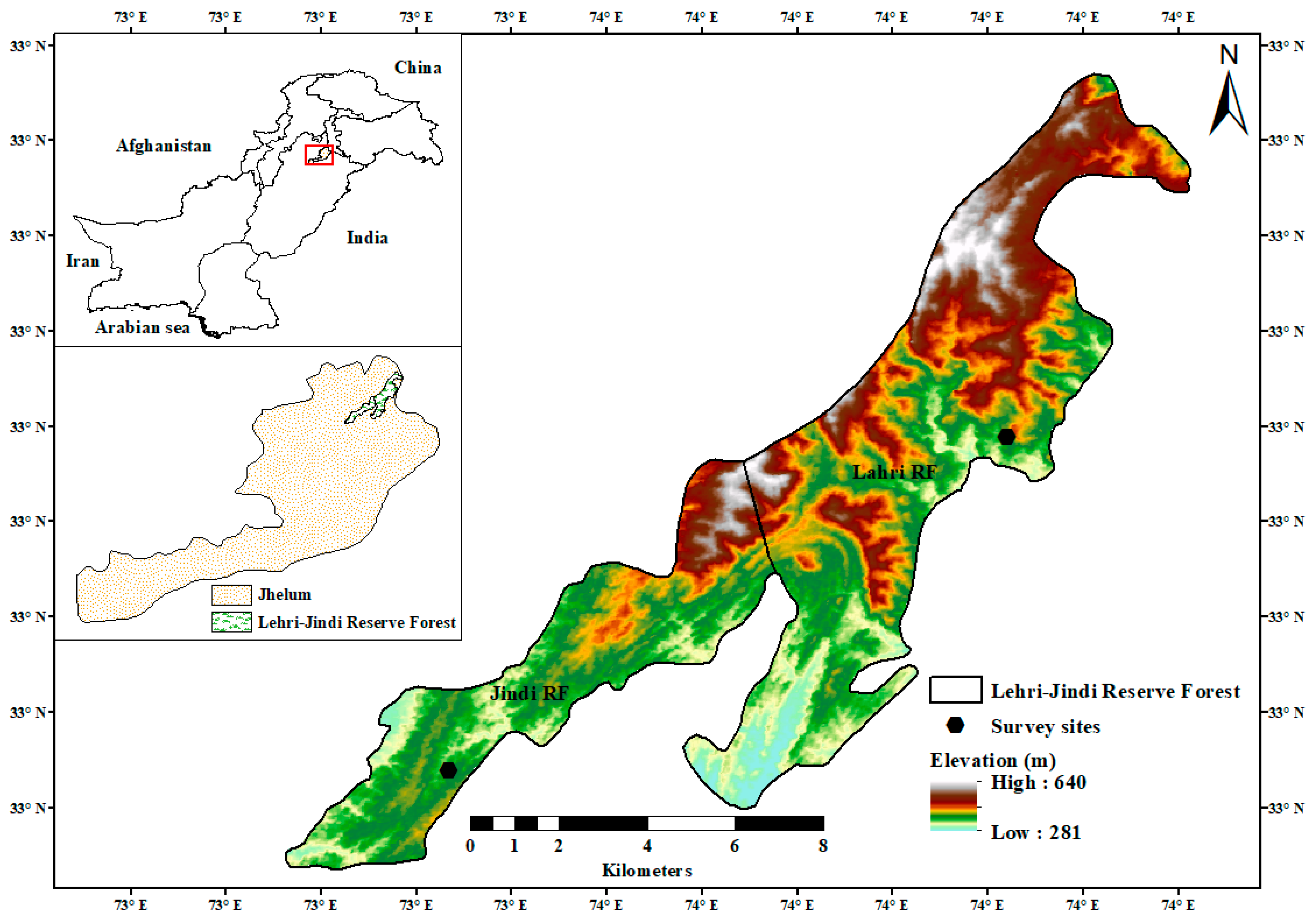
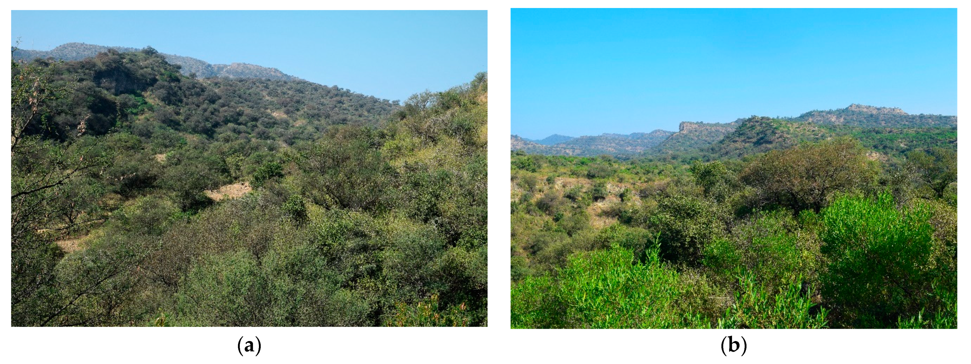
2.1. Site Description
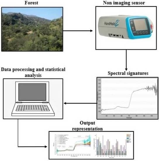
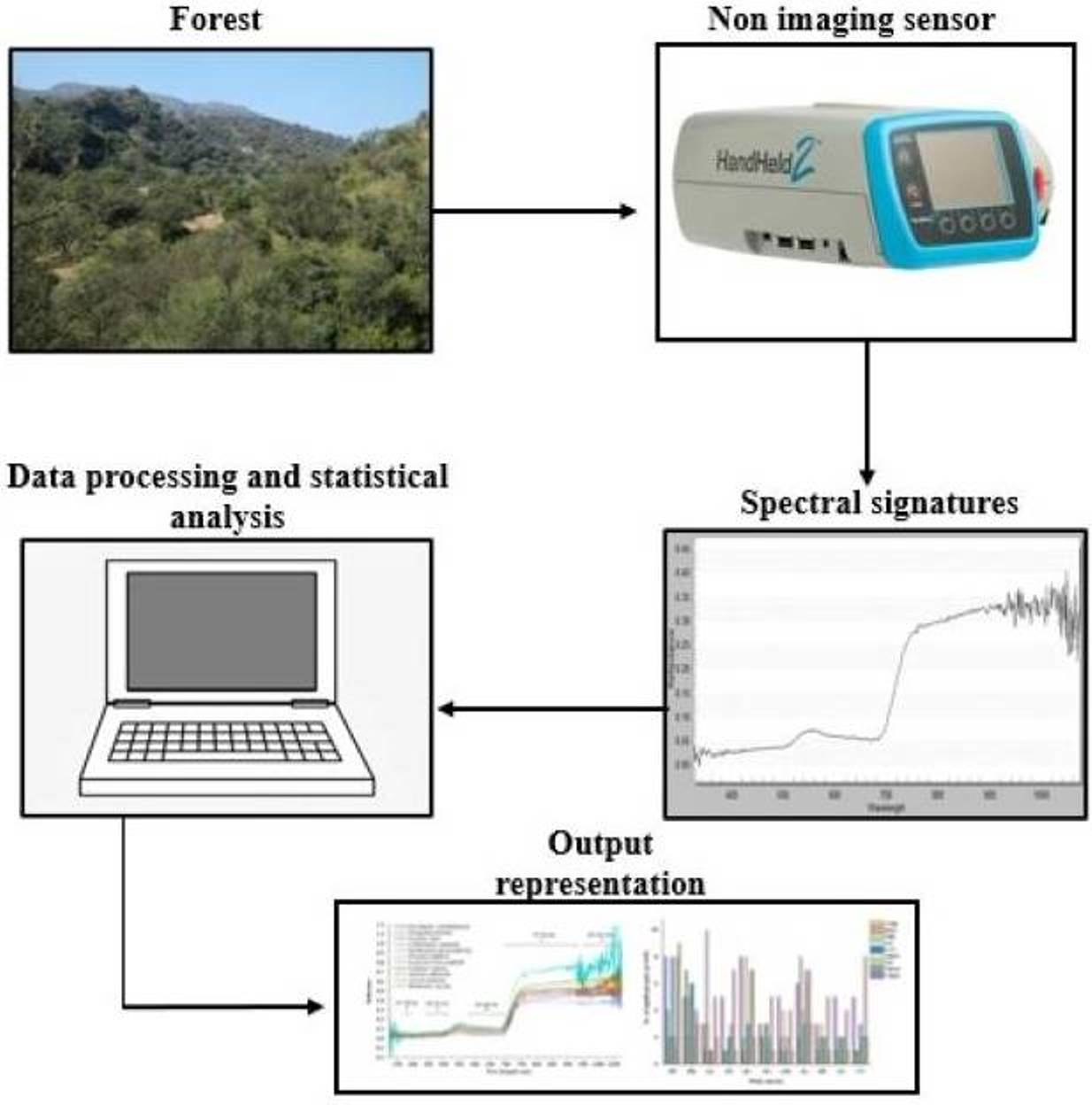
2.2. Field Data Collection
2.2.1. Site Selection and Target Species
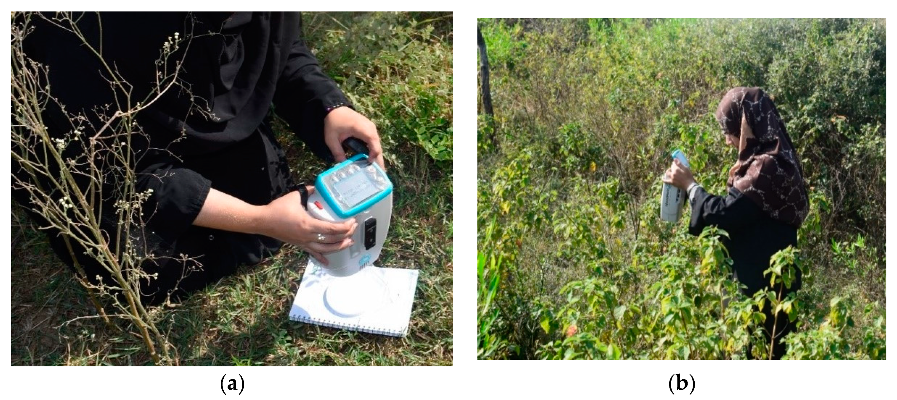
2.2.2. Spectral Sampling
2.3. Processing of Field Spectra
2.4. Calculation of Spectral Indices
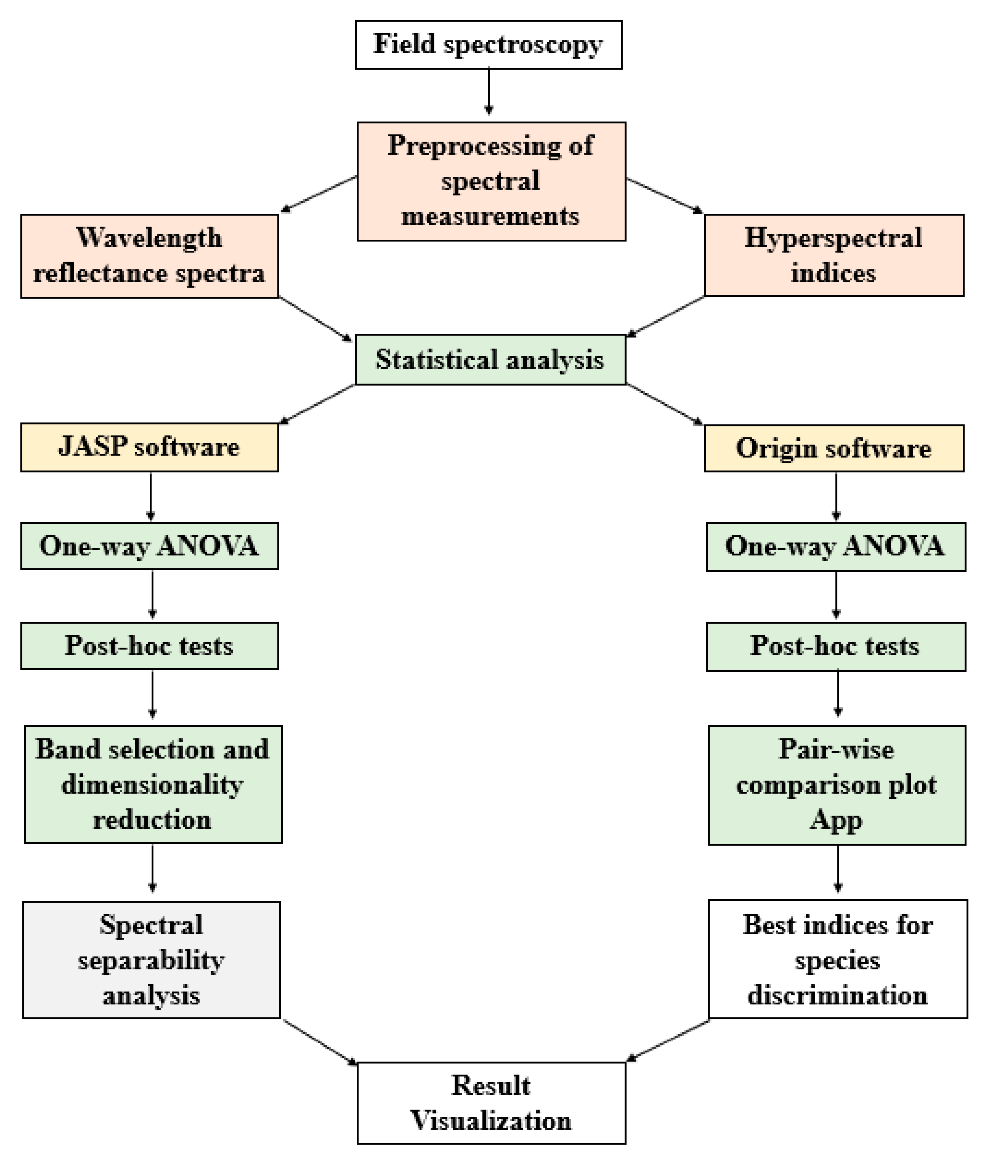
2.5. Statistical Analysis
2.5.1. Spectral Indices
2.5.2. Wavelength Spectra
2.6. Spectral Separability Analysis
3. Results
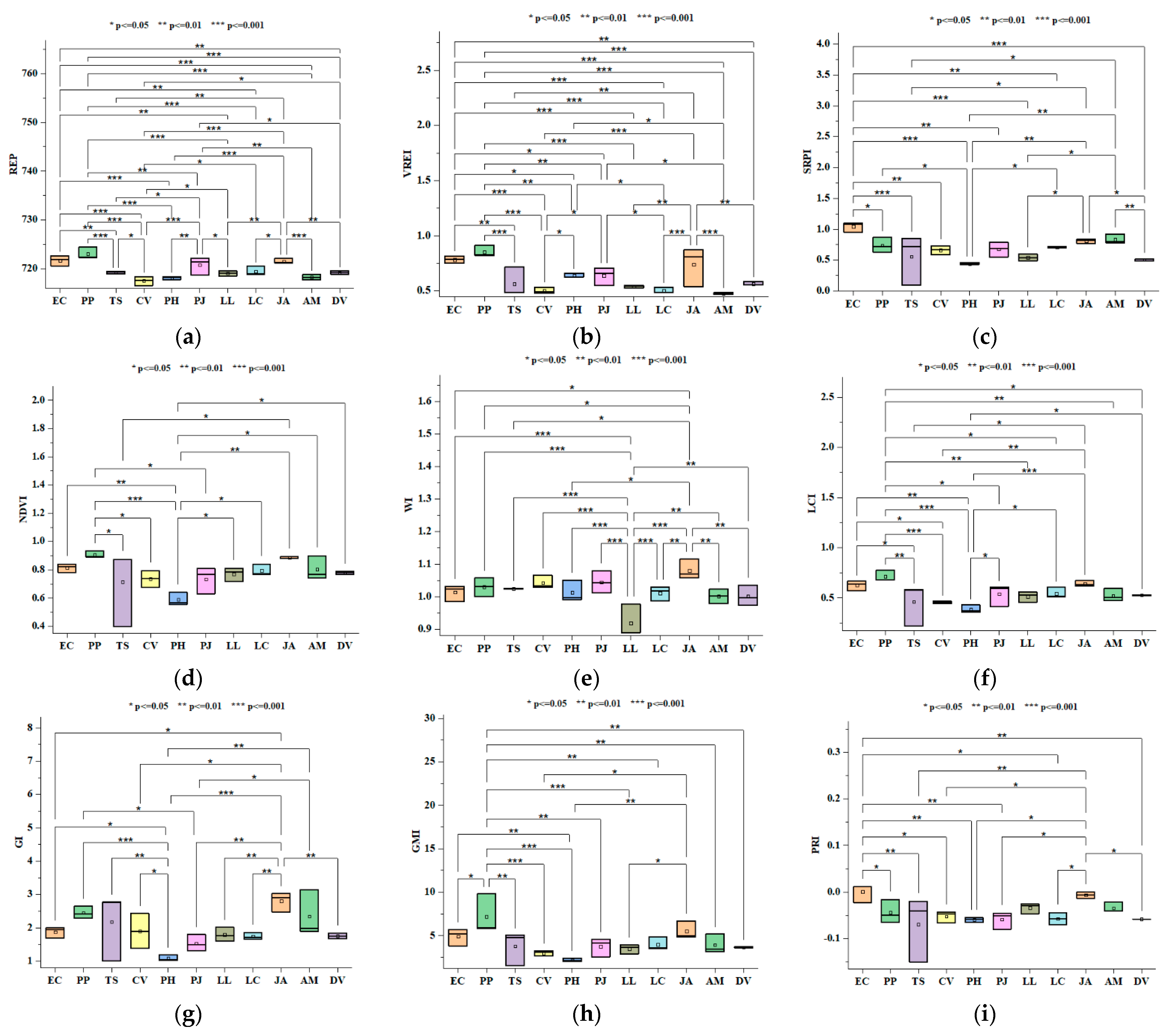
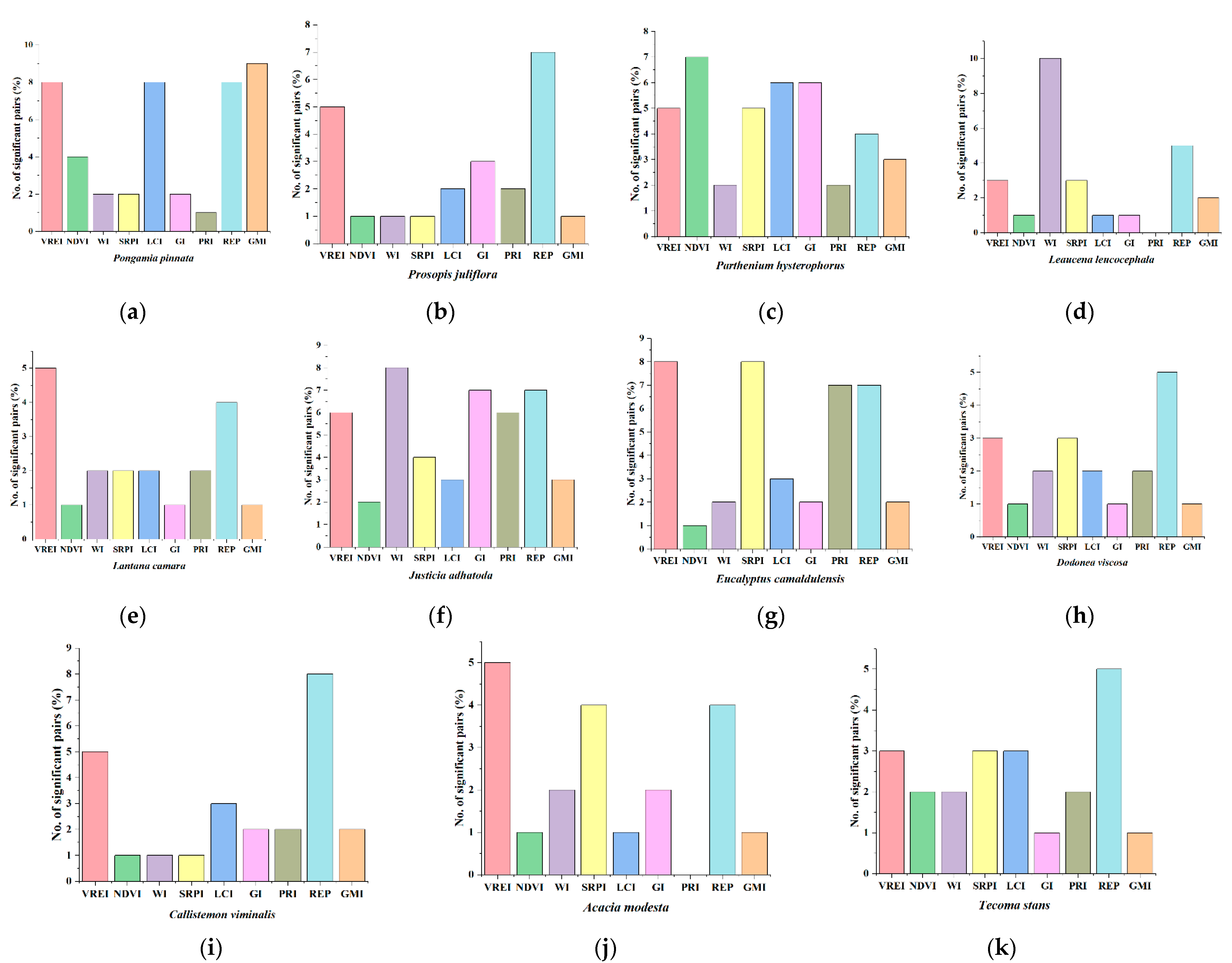
3.1. Spectral Indices
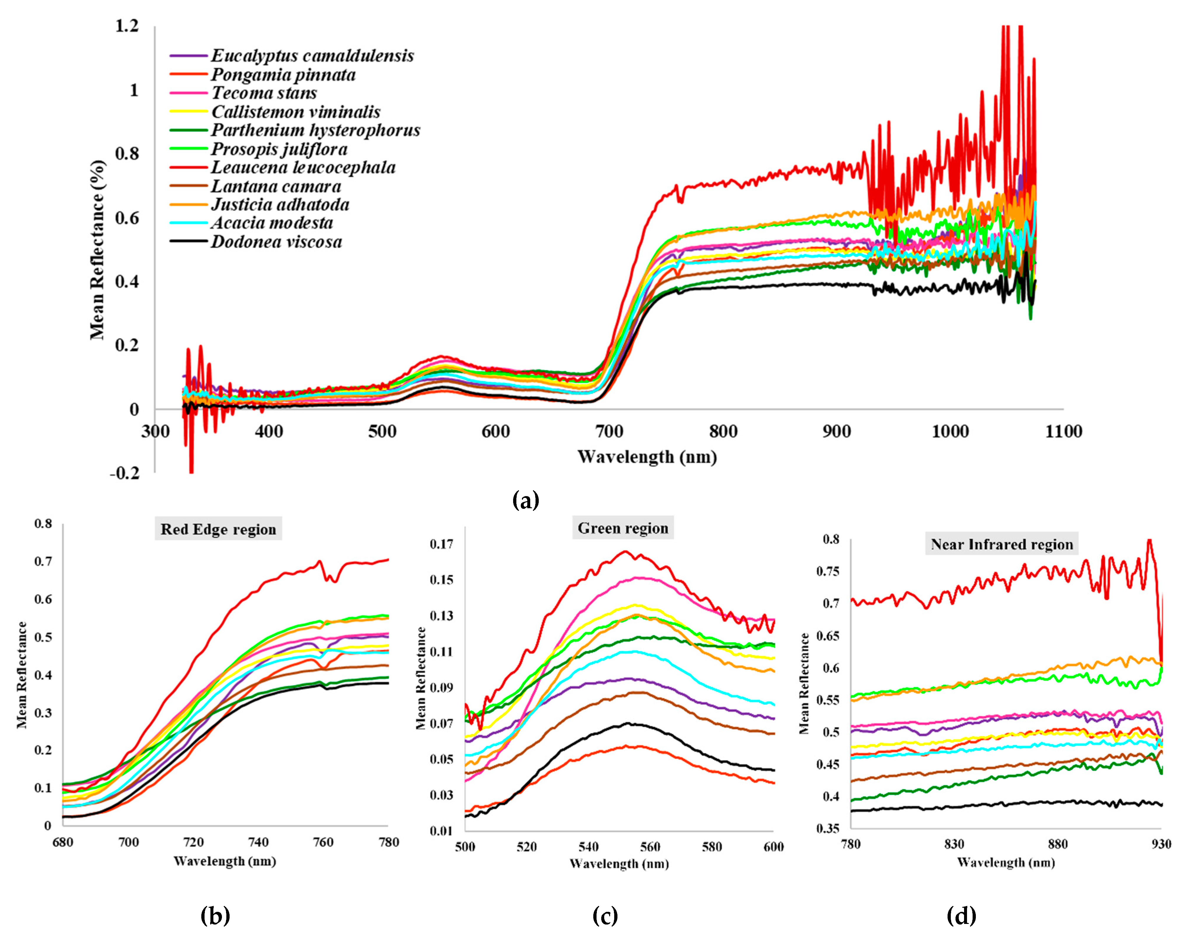
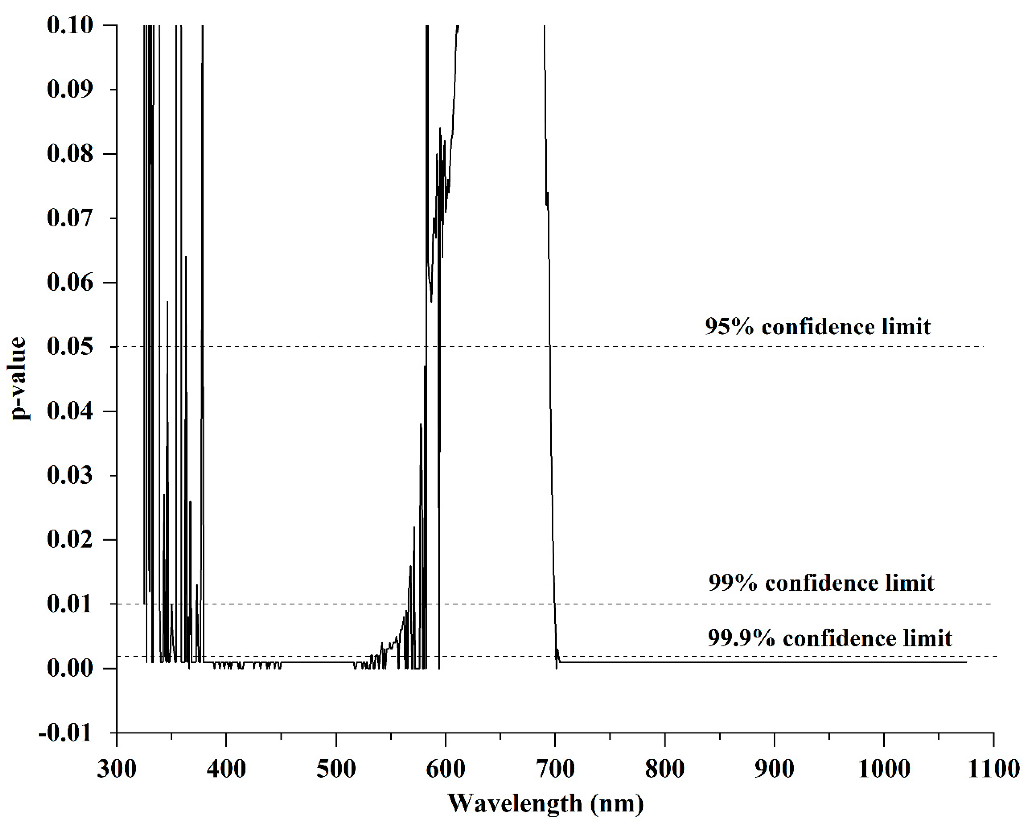
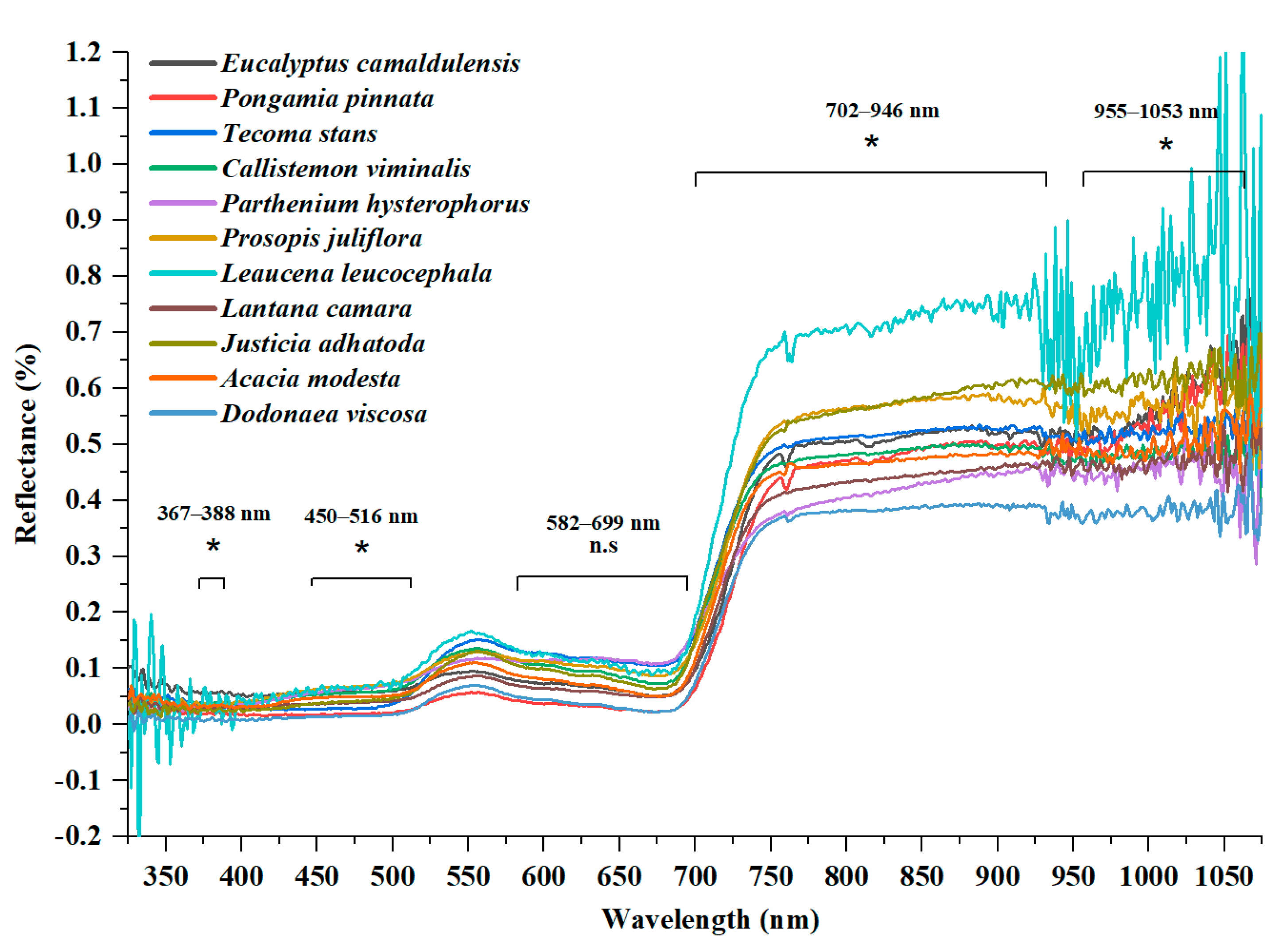
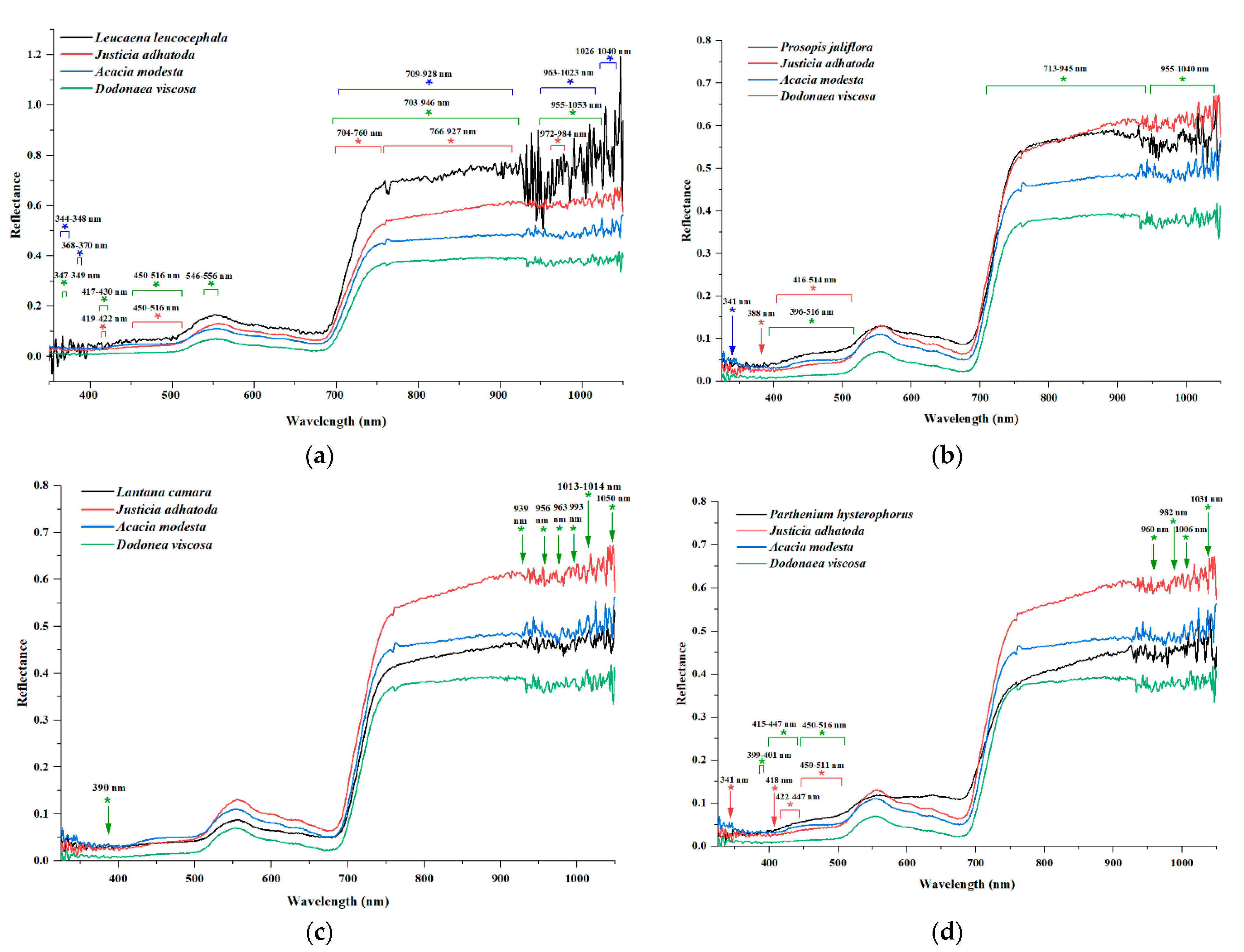
3.2. Wavelength Spectra
3.3. Jeffries–Matusita Distance Analysis
4. Discussion
5. Conclusions
Supplementary Materials
Author Contributions
Funding
Institutional Review Board Statement
Informed Consent Statement
Data Availability Statement
Acknowledgments
Conflicts of Interest
Appendix A

| Plant Pairs | GMI | REP | PRI | GI | LCI | SRPI | WI | NDVI | VREI | Frequency of Different Indices (%) | ||
|---|---|---|---|---|---|---|---|---|---|---|---|---|
| 1 | AM JA | n.s. | *** | n.s. | n.s. | n.s. | n.s. | ** | n.s. | *** | 3 | 33 |
| 2 | AM CV | n.s. | n.s. | n.s. | n.s. | n.s. | n.s. | n.s. | n.s. | n.s. | 0 | 0 |
| 3 | AM EC | n.s. | *** | n.s. | n.s. | n.s. | n.s. | n.s. | n.s. | *** | 2 | 22 |
| 4 | AM LC | n.s. | n.s. | n.s. | n.s. | n.s. | n.s. | n.s. | n.s. | n.s. | 0 | 0 |
| 5 | AM LL | n.s. | n.s. | n.s. | n.s. | n.s. | * | ** | n.s. | n.s. | 3 | 33 |
| 6 | AM PH | n.s. | n.s. | n.s. | ** | n.s. | ** | n.s. | * | * | 5 | 56 |
| 7 | AM PJ | n.s. | ** | n.s. | * | n.s. | n.s. | n.s. | n.s. | * | 3 | 33 |
| 8 | AM PP | ** | *** | n.s. | n.s. | ** | n.s. | n.s. | n.s. | *** | 4 | 44 |
| 9 | AM TS | n.s. | n.s. | n.s. | n.s. | n.s. | * | n.s. | n.s. | n.s. | 1 | 11 |
| 10 | JA CV | * | *** | * | * | ** | n.s. | n.s. | n.s. | *** | 6 | 67 |
| 11 | JA EC | n.s. | n.s. | n.s. | * | n.s. | n.s. | * | n.s. | n.s. | 2 | 22 |
| 12 | JA LC | n.s. | * | * | ** | n.s. | n.s. | ** | n.s. | *** | 5 | 56 |
| 13 | JA LL | * | ** | n.s. | ** | n.s. | * | *** | n.s. | ** | 6 | 67 |
| 14 | JA PH | ** | *** | * | *** | *** | ** | * | ** | n.s. | 8 | 89 |
| 15 | JA PJ | n.s. | n.s. | * | ** | n.s. | n.s. | n.s. | n.s. | n.s. | 2 | 22 |
| 16 | JA PP | n.s. | n.s. | n.s. | n.s. | n.s. | n.s. | * | n.s. | n.s. | 1 | 11 |
| 17 | JA TS | n.s. | ** | ** | n.s. | * | * | * | * | ** | 7 | 78 |
| 18 | CV EC | n.s. | *** | * | n.s. | * | ** | n.s. | n.s. | *** | 5 | 56 |
| 19 | CV PP | *** | *** | n.s. | n.s. | *** | n.s. | n.s. | * | *** | 5 | 56 |
| 20 | CV TS | n.s. | * | n.s. | n.s. | n.s. | n.s. | n.s. | n.s. | n.s. | 1 | 11 |
| 21 | DV AM | n.s. | n.s. | n.s. | n.s. | n.s. | ** | n.s. | n.s. | n.s. | 2 | 22 |
| 22 | DV JA | n.s. | ** | * | ** | n.s. | * | ** | n.s. | ** | 6 | 67 |
| 23 | DV CV | n.s. | * | n.s. | n.s. | n.s. | n.s. | n.s. | n.s. | n.s. | 1 | 11 |
| 24 | DV EC | n.s. | ** | ** | n.s. | n.s. | *** | n.s. | n.s. | ** | 4 | 44 |
| 25 | DV LC | n.s. | n.s. | n.s. | n.s. | n.s. | n.s. | n.s. | n.s. | n.s. | 0 | 0 |
| 26 | DV LL | n.s. | n.s. | n.s. | n.s. | n.s. | n.s. | ** | n.s. | n.s. | 1 | 11 |
| 27 | DV PH | n.s. | n.s. | n.s. | n.s. | * | n.s. | n.s. | * | n.s. | 2 | 22 |
| 28 | DV PJ | n.s. | * | n.s. | n.s. | n.s. | n.s. | n.s. | n.s. | n.s. | 1 | 11 |
| 29 | DV PP | ** | *** | n.s. | n.s. | * | n.s. | n.s. | n.s. | *** | 4 | 44 |
| 30 | DV TS | n.s. | n.s. | n.s. | n.s. | n.s. | n.s. | n.s. | n.s. | n.s. | 0 | 0 |
| 31 | LC CV | n.s. | * | n.s. | n.s. | n.s. | n.s. | n.s. | n.s. | n.s. | 1 | 11 |
| 32 | LC EC | n.s. | ** | * | n.s. | n.s. | ** | n.s. | n.s. | *** | 4 | 44 |
| 33 | LC LL | n.s. | n.s. | n.s. | n.s. | n.s. | n.s. | *** | n.s. | n.s. | 1 | 11 |
| 34 | LC PH | n.s. | n.s. | n.s. | n.s. | * | * | n.s. | * | * | 4 | 44 |
| 35 | LC PJ | n.s. | n.s. | n.s. | n.s. | n.s. | n.s. | n.s. | n.s. | * | 1 | 11 |
| 36 | LC PP | ** | *** | n.s. | n.s. | * | n.s. | n.s. | n.s. | *** | 4 | 44 |
| 37 | LC TS | n.s. | n.s. | n.s. | n.s. | n.s. | n.s. | n.s. | n.s. | n.s. | 0 | 0 |
| 38 | LL CV | n.s. | * | n.s. | n.s. | n.s. | n.s. | *** | n.s. | n.s. | 2 | 22 |
| 39 | LL EC | n.s. | ** | n.s. | n.s. | n.s. | *** | *** | n.s. | *** | 4 | 44 |
| 40 | LL PH | n.s. | n.s. | n.s. | n.s. | n.s. | n.s. | *** | * | n.s. | 2 | 22 |
| 41 | LL PJ | n.s. | * | n.s. | n.s. | n.s. | n.s. | *** | n.s. | n.s. | 2 | 22 |
| 42 | LL PP | *** | *** | n.s. | n.s. | ** | n.s. | *** | n.s. | *** | 5 | 56 |
| 43 | LL TS | n.s. | n.s. | n.s. | n.s. | n.s. | n.s. | *** | n.s. | n.s. | 1 | 11 |
| 44 | PH CV | n.s. | n.s. | n.s. | * | n.s. | n.s. | n.s. | n.s. | * | 2 | 22 |
| 45 | PH EC | ** | *** | ** | * | ** | *** | n.s. | ** | * | 8 | 89 |
| 46 | PH PP | *** | *** | n.s. | *** | *** | * | n.s. | *** | ** | 7 | 78 |
| 47 | PH TS | n.s. | n.s. | n.s. | ** | n.s. | n.s. | n.s. | n.s. | n.s. | 1 | 11 |
| 48 | PJ CV | n.s. | *** | n.s. | n.s. | n.s. | n.s. | n.s. | n.s. | * | 2 | 22 |
| 49 | PJ EC | n.s. | n.s. | ** | n.s. | n.s. | ** | n.s. | n.s. | * | 3 | 33 |
| 50 | PJ PH | n.s. | ** | n.s. | n.s. | * | n.s. | n.s. | n.s. | n.s. | 2 | 22 |
| 51 | PJ PP | ** | ** | n.s. | * | * | n.s. | n.s. | * | ** | 6 | 67 |
| 52 | PJ TS | n.s. | * | n.s. | n.s. | n.s. | n.s. | n.s. | n.s. | n.s. | 1 | 11 |
| 53 | PP EC | * | n.s. | * | n.s. | n.s. | * | n.s. | n.s. | n.s. | 3 | 33 |
| 54 | TS EC | n.s. | ** | ** | n.s. | * | *** | n.s. | n.s. | ** | 5 | 56 |
| 55 | TS PP | ** | *** | n.s. | n.s. | ** | n.s. | n.s. | * | *** | 5 | 56 |
References
- Gallardo, B.; Aldridge, D.C.; González-Moreno, P.; Pergl, J.; Pizarro, M.; Pyšek, P.; Thuiller, W.; Yesson, C.; Vilà, M. Protected areas offer refuge from invasive species spreading under climate change. Glob. Chang. Biol. 2017, 23, 5331–5343. [Google Scholar] [CrossRef] [Green Version]
- Cai, H.; Lu, H.; Tian, Y.; Liu, Z.; Huang, Y.; Jian, S. Effects of invasive plants on the health of forest ecosystems on small tropical coral islands. Ecol. Indic. 2020, 117, 106656. [Google Scholar] [CrossRef]
- Pyšek, P.; Hulme, P.E.; Simberloff, D.; Bacher, S.; Blackburn, T.M.; Carlton, J.T.; Dawson, W.; Essl, F.; Foxcroft, L.C.; Genovesi, P.; et al. Scientists’ warning on invasive alien species. Biol. Rev. 2020, 95, 1511–1534. [Google Scholar] [CrossRef]
- Orr, S.P.; Rudgers, J.A.; Clay, K. Invasive plants can inhibit native tree seedlings: Testing potential allelopathic mechanisms. Plant Ecol. 2005, 181, 153–165. [Google Scholar] [CrossRef]
- Shabbir, A.; Dhileepan, K.; O’Donnell, C.; Adkins, S.W. Complementing biological control with plant suppression: Implications for improved management of parthenium weed (Parthenium hysterophorus L.). Biol. Cont. 2013, 64, 270–275. [Google Scholar] [CrossRef]
- Shabbir, A.; Ali, S.; Khan, I.A.; Belgeri, A.; Khan, N.; Adkins, S. Suppressing parthenium weed with beneficial plants in Australian grasslands. Int. J. Pest Manag. 2021, 67, 114–120. [Google Scholar] [CrossRef]
- Tesfamichael, S.G.; Newete, S.W.; Adam, E.; Dubula, B. Field spectroradiometer and simulated multispectral bands for discriminating invasive species from morphologically similar cohabitant plants. GIsci. Remote Sens. 2018, 55, 417–436. [Google Scholar] [CrossRef]
- Vilà, M.; Espinar, J.L.; Hejda, M.; Hulme, P.E.; Jarošík, V.; Maron, J.L.; Pergl, J.; Schaffner, U.; Sun, Y.; Pyšek, P. Ecological impacts of invasive alien plants: A meta-analysis of their effects on species, communities and ecosystems. Ecol. Lett. 2011, 14, 702–708. [Google Scholar] [CrossRef] [PubMed]
- Pardo-Primoy, D.; Fagúndez, J. Assessment of the distribution and recent spread of the invasive grass Cortaderia selloana in Industrial Sites in Galicia, NW Spain. Flora Morphol. Distrib. Funct. Ecol. Plants 2019, 259, 151465. [Google Scholar] [CrossRef]
- Carlier, J.; Davis, E.; Ruas, S.; Byrne, D.; Caffrey, J.M.; Coughlan, N.E.; Dick, J.T.A.; Lucy, F.E. Using open-source software and digital imagery to efficiently and objectively quantify cover density of an invasive alien plant species. J. Environ. Manag. 2020, 266, 110519. [Google Scholar] [CrossRef] [PubMed]
- Caffrey, J.M.; Baars, J.R.; Barbour, J.H.; Boets, P.; Boon, P.; Davenport, K.; Dick, J.T.A.; Early, J.; Edsman, L.; Gallagher, C.; et al. Tackling invasive alien species in Europe: The top 20 issues. Manag. Biol. Invasions 2014, 5, 1–20. [Google Scholar] [CrossRef] [Green Version]
- Huang, C.Y.; Asner, G.P. Applications of remote sensing to alien invasive plant studies. Sensors 2009, 9, 4869–4889. [Google Scholar] [CrossRef] [Green Version]
- Martin, F.M.; Müllerová, J.; Borgniet, L.; Dommanget, F.; Breton, V.; Evette, A. Using single- and multi-date UAV and satellite imagery to accurately monitor invasive knotweed species. Remote Sens. 2018, 10, 1662. [Google Scholar] [CrossRef] [Green Version]
- Jones, H.G.; Vaughan, R.A. Remote Sensing of Vegetation: Principles, Techniques, and Applications; Oxford University Press: Oxford, UK, 2010; ISBN 0199207798. [Google Scholar]
- Bazzichetto, M.; Malavasi, M.; Bartak, V.; Acosta, A.T.R.; Rocchini, D.; Carranza, M.L. Plant invasion risk: A quest for invasive species distribution modelling in managing protected areas. Ecol. Indic. 2018, 95, 311–319. [Google Scholar] [CrossRef]
- Vaz, A.S.; Alcaraz-Segura, D.; Vicente, J.R.; Honrado, J.P. The many roles of remote sensing in invasion science. Front. Ecol. Evol. 2019, 7, 370. [Google Scholar] [CrossRef] [Green Version]
- Rustamov, R.B.; Hasanova, S.; Zeynalova, M.H. (Eds.) Multi-Purposeful Application of Geospatial Data; IntechOpen: London, UK, 2018. [Google Scholar]
- Xie, Y.; Sha, Z.; Yu, M. Remote sensing imagery in vegetation mapping: A review. J. Plant Ecol. 2008, 1, 9–23. [Google Scholar] [CrossRef]
- Oumar, Z. Assessing the utility of the spot 6 sensor in detecting and mapping Lantana camara for a community clearing project in KwaZulu-Natal, South Africa. S. Afr. J. Geomat. 2016, 5, 214. [Google Scholar] [CrossRef] [Green Version]
- Wang, R.; Gamon, J.A. Remote sensing of terrestrial plant biodiversity. Remote Sens. Environ. 2019, 231, 111218. [Google Scholar] [CrossRef]
- Ismail, R.; Mutanga, O.; Peerbhay, K. The identification and remote detection of alien invasive plants in commercial forests: An Overview. SAJG 2016, 5, 49. [Google Scholar] [CrossRef] [Green Version]
- Matongera, T.N.; Mutanga, O.; Dube, T.; Sibanda, M. Detection and mapping the spatial distribution of bracken fern weeds using the Landsat 8 OLI new generation sensor. Int. J. Appl. Earth Obs. Geoinf. 2017, 57, 93–103. [Google Scholar] [CrossRef]
- Ustin, S.L.; Gamon, J.A. Remote sensing of plant functional types. New Phytol. 2010, 186, 795–816. [Google Scholar] [CrossRef]
- He, K.S.; Rocchini, D.; Neteler, M.; Nagendra, H. Benefits of hyperspectral remote sensing for tracking plant invasions. Divers. Distrib. 2011, 17, 381–392. [Google Scholar] [CrossRef]
- Asner, G.P.; Martin, R.E.; Carlson, K.M.; Rascher, U.; Vitousek, P.M. Vegetation-climate interactions among native and invasive species in Hawaiian rainforest. Ecosystems 2006, 9, 1106–1117. [Google Scholar] [CrossRef]
- Asner, G.P.; Jones, M.O.; Martin, R.E.; Knapp, D.E.; Hughes, R.F. Remote sensing of native and invasive species in Hawaiian forests. Remote Sens. Environ. 2008, 112, 1912–1926. [Google Scholar] [CrossRef]
- Dube, T.; Shoko, C.; Sibanda, M.; Madileng, P.; Maluleke, X.G.; Mokwatedi, V.R.; Tibane, L.; Tshebesebe, T. Remote sensing of invasive Lantana camara (Verbenaceae) in semiarid savanna rangeland ecosystems of South Africa. Rangel. Ecol. Manag. 2020, 73, 411–419. [Google Scholar] [CrossRef]
- Forster, M.; Schmidt, T.; Wolf, R.; Kleinschmit, B.; Fassnacht, F.E.; Cabezas, J.; Kattenborn, T. Detecting the spread of invasive species in central Chile with a Sentinel-2 time-series. In Proceedings of the 9th International Workshop on the Analysis of Multitemporal Remote Sensing Images (MultiTemp), Bruges, Belgium, 27–29 June 2017; pp. 1–4. [Google Scholar]
- Samiappan, S.; Turnage, G.; Hathcock, L.; Casagrande, L.; Stinson, P.; Moorhead, R. Using unmanned aerial vehicles for high-resolution remote sensing to map invasive Phragmites australis in coastal wetlands. Int. J. Remote Sens. 2017, 38, 2199–2217. [Google Scholar] [CrossRef]
- Eitel, J.U.H.; Long, D.S.; Gessler, P.E.; Hunt, E.R.; Brown, D.J. Sensitivity of ground-based remote sensing estimates of wheat chlorophyll content to variation in soil reflectance. Soil Sci. Soc. Am. J. 2009, 73, 1715–1723. [Google Scholar] [CrossRef] [Green Version]
- Niphadkar, M.; Nagendra, H. Remote sensing of invasive plants: Incorporating functional traits into the picture. Int. J. Remote Sens. 2016, 37, 3074–3085. [Google Scholar] [CrossRef]
- Rosso, P.H.; Ustin, S.L.; Hastings, A. Mapping marshland vegetation of San Francisco Bay, California, using hyperspectral data. Int. J. Remote Sens. 2005, 26, 5169–5191. [Google Scholar] [CrossRef]
- Somers, B.; Asner, G.P. Hyperspectral time series analysis of native and invasive species in Hawaiian rainforests. Remote Sens. 2012, 4, 2510–2529. [Google Scholar] [CrossRef] [Green Version]
- Kattenborn, T.; Lopatin, J.; Förster, M.; Braun, A.C.; Fassnacht, F.E. UAV data as alternative to field sampling to map woody invasive species based on combined Sentinel-1 and Sentinel-2 data. Remote Sens. Environ. 2019, 227, 61–73. [Google Scholar] [CrossRef]
- Fernandes, M.R.; Aguiar, F.C.; Silva, J.M.N.; Ferreira, M.T.; Pereira, J.M.C. Spectral discrimination of giant reed (Arundo donax L.): A seasonal study in riparian areas. ISPRS J. Photogramm. Remote Sens. 2013, 80, 80–90. [Google Scholar] [CrossRef]
- Cochrane, M.A. Using vegetation reflectance variability for species level classification of hyperspectral data. Int. J. Remote Sens. 2000, 21, 2075–2087. [Google Scholar] [CrossRef]
- Vaiphasa, C.; Ongsomwang, S.; Vaiphasa, T.; Skidmore, A.K. Tropical mangrove species discrimination using hyperspectral data: A laboratory study. Estuar. Coast. Shelf Sci. 2005, 65, 371–379. [Google Scholar] [CrossRef]
- Ullah, S.; Schlerf, M.; Skidmore, A.K.; Hecker, C. Identifying plant species using mid-wave infrared (2.5–6μm) and thermal infrared (8–14μm) emissivity spectra. Remote Sens. Environ. 2012, 118, 95–102. [Google Scholar] [CrossRef]
- Lehmann, J.; Kuzyakov, Y.; Pan, G.; Ok, Y.S. Biochars and the plant-soil interface. Plant Soil 2015, 395, 1–5. [Google Scholar] [CrossRef]
- Schmidt, K.S.; Skidmore, A.K. Spectral discrimination of vegetation types in a coastal wetland. Remote Sens. Environ. 2003, 85, 92–108. [Google Scholar] [CrossRef]
- Adam, E.; Mutanga, O. Spectral discrimination of papyrus vegetation (Cyperus papyrus L.) in swamp wetlands using field spectrometry. ISPRS J. Photogramm. Remote Sens. 2009, 64, 612–620. [Google Scholar] [CrossRef]
- Aneece, I.; Epstein, H. Identifying invasive plant species using field spectroscopy in the VNIR region in successional systems of north-central Virginia. Int. J. Remote Sens. 2017, 38, 100–122. [Google Scholar] [CrossRef]
- Taylor, S.L.; Hill, R.A.; Edwards, C. Characterising invasive non-native Rhododendron ponticum spectra signatures with spectroradiometry in the laboratory and field: Potential for remote mapping. ISPRS J. Photogramm. Remote Sens. 2013, 81, 70–81. [Google Scholar] [CrossRef]
- Clark, M.L.; Roberts, D.A. Species-level differences in hyperspectral metrics among tropical rainforest trees as determined by a tree-based classifier. Remote Sens. 2012, 4, 1820–1855. [Google Scholar] [CrossRef] [Green Version]
- Ghiyamat, A.; Shafri, H.Z.M.; Shariff, A.R.M. Influence of tree species complexity on discrimination performance of vegetation indices. Eur. J. Remote Sens. 2016, 49, 15–37. [Google Scholar] [CrossRef] [Green Version]
- Rajah, P.; Odindi, J.; Mutanga, O.; Kiala, Z. The utility of Sentinel-2 Vegetation Indices (VIs) and Sentinel-1 Synthetic Aperture Radar The utility of Sentinel-2 Vegetation Indices (VIs) and Sentinel-1 Synthetic Aperture Radar (SAR) for invasive alien species detection and mapping Launched to accelerate biodiversity conservation. Nat. Conserv. 2019, 35, 41–61. [Google Scholar] [CrossRef]
- Cho, M.A.; Sobhan, I.; Skidmore, A.K.; De Leeuw, J. Discriminating species using hyperspectral indices at Leaf and Canopy scales. Int. Arch. Spat. Inf. Sci. 2008, 37, 369–376. [Google Scholar]
- Große-Stoltenberg, A.; Hellmann, C.; Werner, C.; Oldeland, J.; Thiele, J. Evaluation of continuous VNIR-SWIR spectra versus narrowband hyperspectral indices to discriminate the invasive Acacia longifolia within a mediterranean dune ecosystem. Remote Sens. 2016, 8, 334. [Google Scholar] [CrossRef] [Green Version]
- Shahzad, A.; Jamil Hasan Kazmi, S.; Shahid Shaukat, S.; Bin Farhan, S. Mapping invasive plant species in Karachi using high resolution satellite imagery: An object based image analyses approach. Int. J. Biol. Biotech. 2017, 14, 479–484. [Google Scholar]
- Kazmi, J.H.; Haase, D.; Shahzad, A.; Shaikh, S.; Zaidi, S.M.; Qureshi, S. Mapping spatial distribution of invasive alien species through satellite remote sensing in Karachi, Pakistan: An urban ecological perspective. Int. J. Environ. Sci. Technol. 2021, 1–18. [Google Scholar] [CrossRef]
- Nawaz, T.; Hameed, M.; Ashraf, M.; Ahmad, F.; Ahmad, M.S.A.; Hussain, M.; Ahmad, I.; Younis, A.; Ahmad, K.S. Diversity and conservation status of economically important flora of the Salt Range, Pakistan. Pak. J. Bot. 2012, 44, 203–211. [Google Scholar]
- Saad, M.; Anwar, M.; Waseem, M.; Salim, M.; Ali, Z. Distribution range and population status of Indian grey wolf (Canis Lupus Pallipes) and Asiatic jackal (Canis aureus) in Lehri Nature Park, District Jhelum, Pakistan. J. Anim. Plant Sci. 2015, 25, 433–440. [Google Scholar]
- Dai, J.; Roberts, D.A.; Stow, D.A.; An, L.; Hall, S.J.; Yabiku, S.T.; Kyriakidis, P.C. Mapping understory invasive plant species with field and remotely sensed data in Chitwan, Nepal. Remote Sens. Environ. 2020, 250, 1–12. [Google Scholar] [CrossRef]
- Prospere, K.; McLaren, K.; Wilson, B. Plant species discrimination in a tropical wetland using in situ hyperspectral data. Remote Sens. 2014, 6, 8494–8523. [Google Scholar] [CrossRef] [Green Version]
- Mutanga, O.; Skidmore, A.K. Narrow band vegetation indices overcome the saturation problem in biomass estimation. Int. J. Remote Sens. 2004, 25, 3999–4014. [Google Scholar] [CrossRef]
- Gitelson, A.A.; Merzlyak, M.N. Remote estimation of chlorophyll content in higher plant leaves. Int. J. Remote Sens. 1997, 18, 2691–2697. [Google Scholar] [CrossRef]
- Penuelas, J.; Baret, F.; Filella, I. Semi-empirical indices to assess carotenoids/chlorophyll a ratio from leaf spectral reflectance. Photosynthetica 1995, 31, 221–230. [Google Scholar]
- Smith, R.C.G.; Adams, J.; Stephens, D.J.; Hick, P.T. Forecasting wheat yield in a Mediterranean-type environment from the NOAA satellite. Aust. J. Agric. Res. 1995, 46, 113–125. [Google Scholar] [CrossRef]
- Datt, B. Visible/near infrared reflectance and chlorophyll content in eucalyptus leaves. Int. J. Remote Sens. 1999, 20, 2741–2759. [Google Scholar] [CrossRef]
- Merzlyak, M.N.; Gitelson, A.A.; Chivkunova, O.B.; Rakitin, V.Y. Non-destructive optical detection of pigment changes during leaf senescence and fruit ripening. Physiol. Plant. 1999, 106, 135–141. [Google Scholar] [CrossRef] [Green Version]
- Sims, D.A.; Gamon, J.A. Relationships between leaf pigment content and spectral reflectance across a wide range of species, leaf structures and developmental stages. Remote Sens. Environ. 2002, 81, 337–354. [Google Scholar] [CrossRef]
- Vogelmann, J.E.; Rock, B.N.; Moss, D.M. Red edge spectral measurements from sugar maple leaves. Int. J. Remote Sens. 1993, 14, 1563–1575. [Google Scholar] [CrossRef]
- Ganapol, B.D.; Johnson, L.F.; Hammer, P.D.; Hlavka, C.A.; Peterson, D.L. LEAFMOD: A new within-leaf radiative transfer model. Remote Sens. Environ. 1998, 63, 182–193. [Google Scholar] [CrossRef]
- Baranoski, G.V.G.; Rokne, J.G. A practical approach for estimating the red edge position of plant leaf reflectance. Int. J. Remote Sens. 2005, 26, 503–521. [Google Scholar] [CrossRef]
- Pride, M.; Priscilla, M.T.; Gara, T. Dominant wetland vegetation species discrimination and quantification using in situ hyperspectral data. Trans. R. Soc. S. Afr. 2020, 75, 229–238. [Google Scholar] [CrossRef]
- Ferreira, M.P.; Grondona, A.E.B.; Rolim, S.B.A.; Shimabukuro, Y.E. Analyzing the spectral variability of tropical tree species using hyperspectral feature selection and leaf optical modeling. J. Appl. Remote Sens. 2013, 7, 073502. [Google Scholar] [CrossRef]
- Bao, S.; Cao, C.; Chen, W.; Yang, T.; Wu, C. Towards a subtropical forest spectral library: Spectra consistency and spectral separability. Geocarto Int. 2021, 36, 226–240. [Google Scholar] [CrossRef]
- Schmidt, K.S.; Skidmore, A.K. Exploring spectral discrimination of grass species in African rangelands. Int. J. Remote Sens. 2001, 22, 3421–3434. [Google Scholar] [CrossRef]
- Das, B.; Sahoo, R.N.; Biswas, A.; Pargal, S.; Krishna, G.; Verma, R.; Chinnusamy, V.; Sehgal, V.K.; Gupta, V.K. Discrimination of rice genotypes using field spectroradiometry. Geocarto Int. 2020, 35, 64–77. [Google Scholar] [CrossRef]
- Richards, J.A.; Jia, X. Remote Sensing Digital Image Analysis: An Introduction; Springer: Berlin, Germany, 1999. [Google Scholar]
- Richards, J.A. Remote Sensing Digital Image Analysis: An Introduction; Springer: New York, NY, USA, 1993. [Google Scholar]
- R Core Team. R: A Language and Environment for Statistical Computing. Available online: https://www.r-project.org/ (accessed on 10 September 2021).
- Mutanga, O.; Ismail, R.; Ahmed, F.; Kumar, L. Using insitu hyperspectral remote sensing to discriminate pest attacked pine forests in South Africa. In Proceedings of the 28th Asian Conference on Remote Sensing, Kuala Lumpur, Malaysia, 12–16 November 2007; pp. 2089–2094. [Google Scholar]
- Shafri, H.Z.M.; Anuar, M.I.; Seman, I.A.; Noor, N.M. Spectral discrimination of healthy and ganoderma-infected oil palms from hyperspectral data. Int. J. Remote Sens. 2011, 32, 7111–7129. [Google Scholar] [CrossRef]
- Santos, M.J.; Ustin, S.L. Spectral identification of native and non-native plant species for biodiversity assessments. In Proceedings of the International Geoscience and Remote Sensing Symposium (IGARSS), Valencia, Spain, 22–27 July 2018; pp. 3420–3423. [Google Scholar]
- Chance, C.M.; Coops, N.C.; Plowright, A.A.; Tooke, T.R.; Christen, A.; Aven, N. Invasive shrub mapping in an urban environment from hyperspectral and LiDAR-derived attributes. Front. Plant Sci. 2016, 7, 1–19. [Google Scholar] [CrossRef] [Green Version]
- Panigrahy, S.; Kumar, T.; Manjunath, K.R. Hyperspectral leaf signature as an added dimension for species discrimination: Case study of four tropical mangroves. Wetl. Ecol. Manag. 2012, 20, 101–110. [Google Scholar] [CrossRef]
- Roberts, D.A.; Ustin, S.L.; Ogunjemiyo, S.; Greenberg, J.; Bobrowski, S.Z.; Chen, J.; Hinckley, T.M. Spectral and structural measures of northwest forest vegetation at leaf to landscape scales. Ecosystems 2004, 7, 545–562. [Google Scholar] [CrossRef]
- Gholizadeh, A.; Mišurec, J.; Kopačková, V.; Mielke, C.; Rogass, C. Assessment of red-edge position extraction techniques: A case study for norway spruce forests using hymap and simulated sentinel-2 data. Forests 2016, 7, 226. [Google Scholar] [CrossRef] [Green Version]
- Clevers, J.G.P.W.; De Jong, S.M.; Epema, G.F.; Van Der Meer, F.; Bakker, W.H.; Skidmore, A.K.; Addink, E.A. MERIS and the red-edge position. Int. J. App. Earth Obs. Geoinf. 2001, 3, 313–320. [Google Scholar] [CrossRef]
- Otunga, C.; Odindi, J.; Mutanga, O.; Adjorlolo, C. Evaluating the potential of the red edge channel for C3 (Festuca spp.) grass discrimination using Sentinel-2 and Rapid Eye satellite image data. Geocarto Int. 2019, 34, 1123–1143. [Google Scholar] [CrossRef]
- Rouse, J.W.; Hass, R.H.; Schell, J.A.; Deering, D.W. Monitoring Vegetation Systems in the Great Plains with ERTS; NASA Special Publication: Washington, DC, USA, 1974. [Google Scholar]
- Tucker, C.J. Red and photographic infrared linear combinations for monitoring vegetation. Remote Sens. Environ. 1979, 8, 127–150. [Google Scholar] [CrossRef] [Green Version]
- Bratsch, S.N.; Epstein, H.E.; Buchhorn, M.; Walker, D.A. Differentiating among four Arctic tundra plant communities at Ivotuk, Alaska using field spectroscopy. Remote Sens. 2016, 8, 51. [Google Scholar] [CrossRef] [Green Version]
- Chen, J.M. Evaluation of vegetation indices and a modified simple ratio for boreal applications. Can. J. Remote Sens. 1996, 22, 229–242. [Google Scholar] [CrossRef]
- Ren, S.; Chen, X.; An, S. Assessing plant senescence reflectance index-retrieved vegetation phenology and its spatiotemporal response to climate change in the Inner Mongolian Grassland. Int. J. Biometeorol. 2017, 61, 601–612. [Google Scholar] [CrossRef]
- Thenkabail, P.S.; Mariotto, I.; Gumma, M.K.; Middleton, E.M.; Landis, D.R.; Huemmrich, K.F. Selection of hyperspectral narrowbands (hnbs) and composition of hyperspectral twoband vegetation indices (HVIS) for biophysical characterization and discrimination of crop types using field reflectance and hyperion/EO-1 data. IEEE J. Sel. Top. Appl. Earth Obs. Remote Sens. 2013, 6, 427–439. [Google Scholar] [CrossRef] [Green Version]
- Jiménez, M.; Díaz-Delgado, R. Towards a standard plant species spectral library protocol for vegetation mapping: A case study in the shrubland of Doñana National Park. ISPRS Int. J. Geo-Inf. 2015, 4, 2472–2495. [Google Scholar] [CrossRef] [Green Version]
- Kganyago, M.; Odindi, J.; Adjorlolo, C.; Mhangara, P. Selecting a subset of spectral bands for mapping invasive alien plants: A case of discriminating parthenium hysterophorus using field spectroscopy data. Int. J. Remote Sens. 2017, 38, 5608–5625. [Google Scholar] [CrossRef]
- Thenkabail, P.S.; Enclona, E.A.; Ashton, M.S.; Van Der Meer, B. Accuracy assessments of hyperspectral waveband performance for vegetation analysis applications. Remote Sens. Environ. 2004, 91, 354–376. [Google Scholar] [CrossRef]
- Thomson, E.R.; Spiegel, M.P.; Althuizen, I.H.J.; Bass, P.; Chen, S.; Chmurzynski, A.; Halbritter, A.H.; Henn, J.J.; Jónsdóttir, I.S.; Klanderud, K.; et al. Multiscale mapping of plant functional groups and plant traits in the High Arctic using field spectroscopy, UAV imagery and Sentinel-2A data. Environ. Res. Lett. 2021, 16, 55006. [Google Scholar] [CrossRef]
- Mutanga, O.; Skidmore, A.K. Red edge shift and biochemical content in grass canopies. ISPRS J. Photogramm. Remote Sens. 2007, 62, 34–42. [Google Scholar] [CrossRef]
- Filella, I.; Peñuelas, J. The red edge position and shape as indicators of plant chlorophyll content, biomass and hydric status. Int. J. Remote Sens. 1994, 15, 1459–1470. [Google Scholar] [CrossRef]
- Asner, G.P.; Martin, R.E.; Suhaili, A. Bin Sources of Canopy Chemical and Spectral Diversity in Lowland Bornean Forest. Ecosystems 2012, 15, 504–517. [Google Scholar] [CrossRef]
- Zhang, J.; Rivard, B.; Sánchez-Azofeifa, A.; Castro-Esau, K. Intra- and inter-class spectral variability of tropical tree species at La Selva, Costa Rica: Implications for species identification using HYDICE imagery. Remote Sens. Environ. 2006, 105, 129–141. [Google Scholar] [CrossRef]
- Xiao, Y.; Zhao, W.; Zhou, D.; Gong, H. Sensitivity analysis of vegetation reflectance to biochemical and biophysical variables at leaf, canopy, and regional scales. IEEE Trans. Geosci. Remote Sens. 2014, 52, 4014–4024. [Google Scholar] [CrossRef]
- Thenkabail, P.S.; Smith, R.B.; De Pauw, E. Evaluation of narrowband and broadband vegetation indices for determining optimal hyperspectral wavebands for agricultural crop characterization. Photogramm. Eng. Remote Sens. 2002, 68, 607–621. [Google Scholar]
- Lewis, M. Spectral characterization of Australian arid zone plants. Can. J. Remote Sens. 2002, 28, 219–230. [Google Scholar] [CrossRef]
- Smith, A.M.; Blackshaw, R.E. Weed: Crop Discrimination Using Remote Sensing: A Detached Leaf Experiment. Weed Technol. 2003, 17, 811–820. [Google Scholar] [CrossRef]
- Mutanga, O.; Skidmore, A.K.; Prins, H.H.T. Predicting in situ pasture quality in the Kruger National Park, South Africa, using continuum-removed absorption features. Remote Sens. Environ. 2004, 89, 393–408. [Google Scholar] [CrossRef]
- Richards, J.A. Remote Sensing Digital Image Analysis: An Introduction; Springer: Berlin/Heidelberg, Germany, 2013; Volume 9783642300, ISBN 9783642300622. [Google Scholar]
- Dabboor, M.; Howell, S.; Shokr, M.; Yackel, J. The Jeffries–Matusita distance for the case of complex Wishart distribution as a separability criterion for fully polarimetric SAR data. Int. J. Remote Sens. 2014, 35, 6859–6873. [Google Scholar] [CrossRef]
- Jacobsen, A.; Jacobsen, A.; Nielsen, A.; Ejmais, R.; Groom, G.B. Spectral identification of plant communities for mapping of semi-natural grasslands. Can. J. Remote Sens. 2000, 26, 370–383. [Google Scholar] [CrossRef] [Green Version]
- Ma, N.; Hu, Y.F.; Zhuang, D.F.; Wang, X.S. Determination on the optimum band combination of HJ-1A hyperspectral data in the case region of dongguan based on optimum index factor and J–M distance. Remote Sens. Technol. Appl. 2010, 25, 358–365. [Google Scholar]
- Torbick, N.; Becker, B.; Qi, J.; Lusch, D. Characterizing Field-Level Hyperspectral Measurements for Identifying Wetland Invasive Plant Species; Nova Science Publishers: New York, NY, USA, 2009; pp. 97–115. [Google Scholar]


| Category | Plant Species | Common Name | Family | Habit |
|---|---|---|---|---|
| Native | Justicia adhatoda L. | Malabar nut | Acanthaceae | shrub |
| Acacia modesta Wall. | Hook thorn tree | Fabaceae | tree | |
| Dodonaea viscosa (L.) Jacq. | Switch sorrel | Sapindaceae | shrub | |
| Invasive | Parthenium hysterophorus L. | Carrot grass | Asteraceae | herb |
| Prosopis juliflora (Sw.) DC. | Mesquite | Fabaceae | tree | |
| Leucaena leucocephala (Lam.) de Wit | White lead tree | Fabaceae | tree | |
| Lantana camara L. | Red sage | Verbenaceae | shrub | |
| Ornamental | Eucalyptus camaldulensis Dehnh. | River red gum | Myrtaceae | tree |
| Pongamia pinnata (L.) Pierre | Pogam oil tree | Fabaceae | tree | |
| Tecoma stans (L.) Juss. ex Kunth | Yellow trumpet bush | Bignoniaceae | shrub | |
| Callistemon viminalis (Sol. ex Gaertn.) G.Don | Bottle brush | Myrtaceae | tree |
| Narrowband Spectral Indices | Equations | Significance | Reference |
|---|---|---|---|
| Narrow-banded NDVI = Normalised difference vegetation index | (R830–R670)/ (R830 + R670) | Canopy greenness, leaf area index, fraction of photosynthetically active radiation | [55] |
| GMI = Gitelson and Merzylak index | (R750)/(R700) | Chlorophyll content | [56] |
| PRI= Photochemical reflectance index | (R531− R570)/ (R531 + R570) | Conversion of xanthophylls-cycle pigments, photosynthetic light use efficiency, LAI | [57] |
| GI = Greenness index | R554/R677 | Indicator of prolonged vegetation stress due to changes in canopy structure | [58] |
| LCI = Leaf Chlorophyll Index | (R850−R710)/ (R850 + R680) | Total chlorophyll content | [59] |
| SRPI = Simple Ratio Pigment Index | (R430)/(R680) | Carotenoid/chlorophyll-a content | [57] |
| WI = Water Index | (R900)/(R970) | Water status | [57] |
| PSRI = Plant Senescing Reflectance Index | (R678–R500) /R750 | Leaf Senescence | [60] |
| mSR = modified Simple Ratio | (R800–R445)/ (R680–R445) | Chlorophyll | [61] |
| VREI = Vogelmann Red-Edge Index | (R734-R747)/ (R715-R726) | Chlorophyll concentration, canopy leaf area, and water content | [62] |
| REP = Red-Edge Position | Indicator of sharp change in leaf reflectance | [63,64] |
| Plant Category | Plant Species | NDVI * | GMI ** | GI ** | PRI * | PSRI n.s | LCI ** | WI *** | SRPI ** | mSR n.s | REP *** | VREI *** |
|---|---|---|---|---|---|---|---|---|---|---|---|---|
| Ornamental | Eucalyptuscamaldulensis (EC) | 0.81 | 4.91 | 1.87 | 0 | −0.02 | 0.626 | 1.013 | 1.043 | 20.73 | 721.73 | 0.78 |
| Pongamia pinnata (PP) | 0.91 | 7.17 | 2.45 | −0.04 | 0.01 | 0.713 | 1.029 | 0.738 | 78.66 | 723.03 | 0.854 | |
| Tecoma stans (TS) | 0.72 | 3.80 | 2.18 | −0.07 | 0.15 | 0.462 | 1.024 | 0.555 | 53.28 | 719.26 | 0.563 | |
| Callistemon viminalis (CV) | 0.74 | 3.00 | 1.90 | −0.05 | 0.03 | 0.455 | 1.042 | 0.663 | 23.02 | 717.54 | 0.503 | |
| Invasive | Parthenium hysterophorus (PH) | 0.59 | 2.18 | 1.09 | −0.06 | 0.10 | 0.387 | 1.012 | 0.443 | 6.67 | 718.14 | 0.638 |
| Prosopis juliflora (PJ) | 0.74 | 3.78 | 1.53 | −0.06 | 0.03 | 0.542 | 1.044 | 0.676 | 31.59 | 720.79 | 0.639 | |
| Leaucena leucocephala (LL) | 0.77 | 3.48 | 1.79 | −0.03 | 0.02 | 0.516 | 0.918 | 0.546 | 18.29 | 719.1 | 0.540 | |
| Lantana camara (LC) | 0.79 | 3.97 | 1.74 | −0.06 | 0.02 | 0.544 | 1.011 | 0.706 | 34.86 | 719.47 | 0.503 | |
| Native | Justicia adhatoda (JA) | 0.89 | 5.52 | 2.80 | −0.01 | 0.003 | 0.642 | 1.080 | 0.807 | 93.63 | 721.54 | 0.741 |
| Acacia modesta (AM) | 0.80 | 3.92 | 2.34 | −0.03 | −0.001 | 0.524 | 1.001 | 0.833 | 123.13 | 718.27 | 0.478 | |
| Dodonea viscosa (DV) | 0.78 | 3.67 | 1.75 | −0.06 | 0.038 | 0.528 | 1.001 | 0.504 | 16.65 | 719.23 | 0.565 |
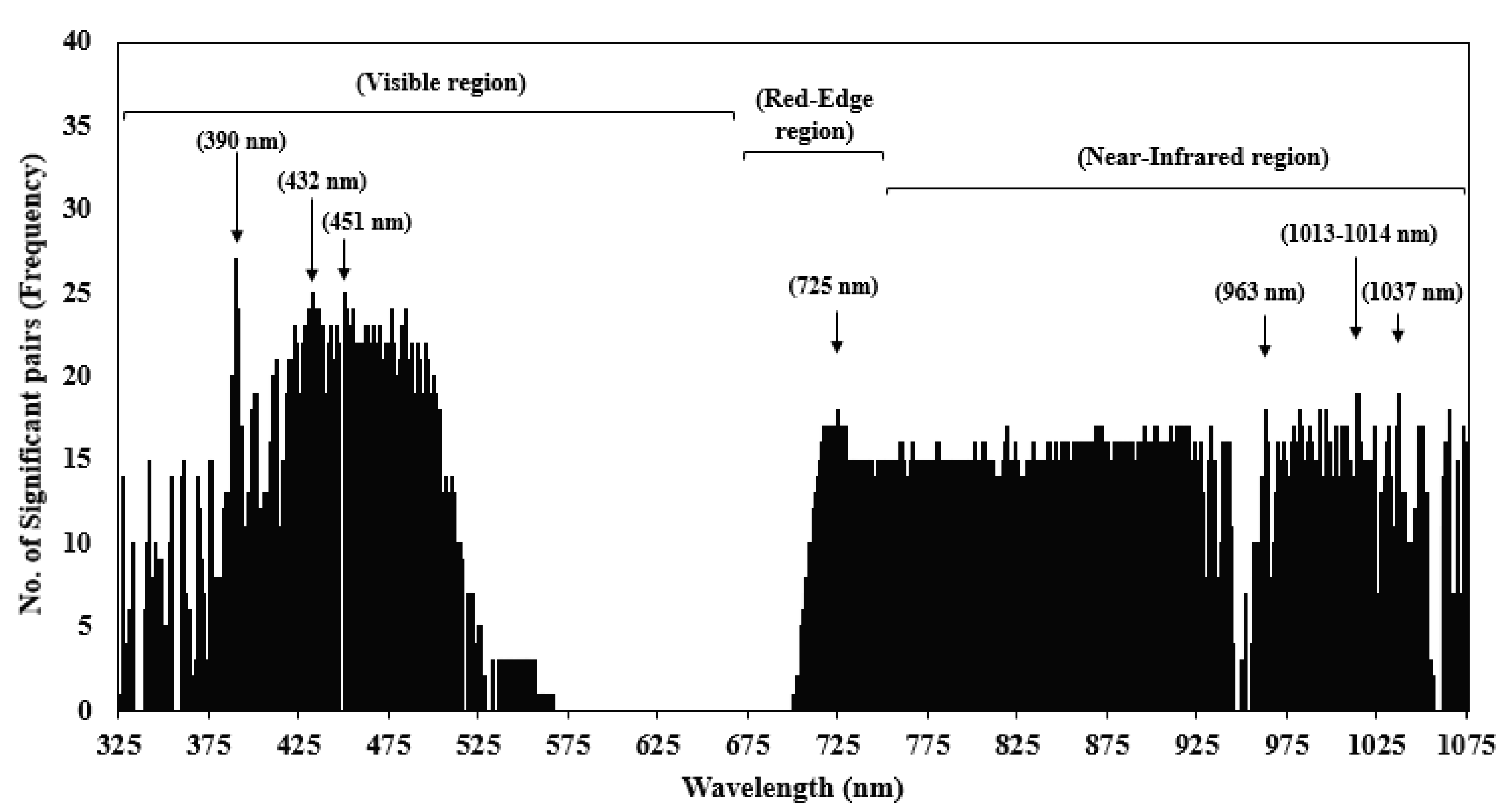
| Wavelength Region | Description | Total No. of Bands | Significant Bands (p < 0.05) | Non Significant Bands | Frequency |
|---|---|---|---|---|---|
| 325–680 nm | Visible region | 356 | 199 | 157 | 56% |
| 681–750 nm | Red-edge region | 70 | 50 | 20 | 71.4% |
| 751–1075 nm | NIR region | 325 | 313 | 12 | 96% |
| 325–1075 nm | Whole spectrum | 751 | 562 | 189 | 75% |
| Plant Category | Plant Pairs | Significant Bands (%) | |||
|---|---|---|---|---|---|
| Visible 325–680 nm | Red-Edge 681–750 nm | Near Infrared 751–1075 nm | Full Spectrum 325–1075 nm | ||
| Invasive | LC vs. AM | 0 (0) | 0 | 0 | 0 |
| LC vs. CV | 2 (0.56) | 0 | 6 (1.85) | 8 (1.07) | |
| LC vs. DV | 1 (0.28) | 0 | 11(3.38) | 12 (1.60) | |
| LC vs. EC | 48 (13.48) | 0 | 0 | 48 (6.39) | |
| LC vs. LL | 84 (23.60) | 46 (65.71) | 284 (87.38) | 414 (55.13) | |
| LC vs. PH | 7 (1.97) | 0 | 0 | 7 (0.93) | |
| LC vs. PJ | 68 (19.10) | 0 | 0 | 68 (9.05) | |
| LC vs. PP | 0 | 0 | 4 (1.23) | 4 (0.53) | |
| LC vs. TS | 0 | 0 | 0 | 0 | |
| LC vs. JA | 0 | 0 | 0 | 0 | |
| LL vs. JA | 122 (34.27) | 47 (67.14) | 258 (79.38) | 427 (56.86) | |
| LL vs. CV | 25 (7.02) | 35 (50.00) | 277 (85.23) | 337 (44.87) | |
| LL vs. DV | 150 (42.13) | 48 (68.57) | 307 (94.46) | 505 (67.24) | |
| LL vs. EC | 36 (10.11) | 47 (67.14) | 257 (79.08) | 340 (45.27) | |
| LL vs. PH | 26 (7.30) | 40 (57.14() | 290 (89.23) | 356 (47.40) | |
| LL vs. PJ | 28 (7.87) | 36 (51.43) | 126 (38.77) | 190 (25.30) | |
| LL vs. PP | 160 (44.64) | 50 (71.43) | 262 (80.62) | 472 (62.85) | |
| LL vs. TS | 108 (30.34) | 31 (44.29) | 267 (82.15) | 406 (54.06) | |
| LL vs. AM | 27 (7.58) | 42 (60.00) | 278 (85.54) | 347 (46.21) | |
| PH vs. AM | 0 | 0 | 0 | 0 | |
| PH vs. CV | 1 (0.28) | 0 | 1 (0.31) | 2 (0.27) | |
| PH vs. DV | 104 (29.21) | 0 | 6 (1.85) | 110 (14.65) | |
| PH vs. EC | 26 (7.30) | 0 | 10 (3.08) | 36 (4.79) | |
| PH vs. PJ | 0 | 2 (2.86) | 62 (19.08) | 64 (8.52) | |
| PH vs. PP | 106 (29.78) | 0 | 3 (0.92) | 109 (14.51) | |
| PH vs. TS | 75(21.07) | 0 | 1 (0.31) | 76 (10.12) | |
| PH vs. JA | 84 (23.60) | 0 | 0 | 84 (11.19) | |
| PJ vs. AM | 1 (0.28) | 0 | 0 | 1 (0.13) | |
| PJ vs. JA | 95 (26.69) | 0 | 0 | 95 (12.65) | |
| PJ vs. CV | 1 (0.28) | 0 | 0 | 1 (0.13) | |
| PJ vs. DV | 116 (32.58) | 38 (54.29) | 284 (87.38) | 438 (58.32) | |
| PJ vs. EC | 6 (1.69) | 0 | 1 (0.31) | 6 (0.08) | |
| PJ vs. PP | 117 (32.87) | 18 (25.71) | 1 (0.31) | 136 (18.11) | |
| PJ vs. TS | 84 (23.60) | 0 | 0 | 84 (11.19) | |
| Native | AM vs. PP | 79 (22.19) | 0 | 0 | 79 (10.52) |
| AM vs. TS | 0 | 0 | 0 | 0 | |
| AM vs. JA | 3 (0.84) | 0 | 0 | 3 (0.40) | |
| AM vs. CV | 0 | 0 | 0 | 0 | |
| AM vs. DV | 24 (6.74) | 22 (31.43) | 79 (24.31) | 125 (16.64) | |
| AM vs. EC | 32 (8.99) | 0 | 1 (0.31) | 3 (0.40) | |
| JA vs. CV | 40 (11.24) | 0 | 0 | 40 (5.33) | |
| JA vs. TS | 1 (0.28) | 0 | 0 | 1 (0.13) | |
| JA vs. DV | 1 (0.28) | 26 (37.14) | 270 (83.08) | 297 (39.55) | |
| JA vs. EC | 111 (31.18) | 0 | 4 (1.23) | 115 (15.31) | |
| JA vs. PP | 0 | 0 | 0 | 0 | |
| DV vs. CV | 110 (30.90) | 42 (60.00) | 202 (62.15) | 354 (47.14) | |
| DV vs. EC | 132 (37.08) | 12 (17.15) | 294 (90.46) | 438 (58.32) | |
| DV vs. PP | 2 (0.56) | 0 | 212 (65.23) | 214 (28.50) | |
| DV vs. TS | 7 (1.97) | 44 (62.86) | 261 (80.31) | 312 (41.54) | |
| Ornamental | CV vs. EC | 8 (2.25) | 0 | 0 | 8 (1.07) |
| CV vs. PP | 119 (33.43) | 19 (27.14) | 4 (1.23) | 142 (18.91) | |
| CV vs. TS | 61 (17.13) | 0 | 0 | 61 (8.12) | |
| EC vs. PP | 137 (38.48) | 0 | 0 | 137 (18.24) | |
| EC vs. TS | 89 (25.00) | 6 (8.57) | 2 (0.62) | 97 (12.92) | |
| PP vs. TS | 21 (5.90) | 26 (37.14) | 2 (0.62) | 49 (6.52) | |
| Spectrum Region (325–1075 nm) | Wavelengths Selected (nm) | No. of Most Significant Wavelengths |
|---|---|---|
| Visible region (325–680 nm) | 390, 432, 433, 451 | 4 |
| Red-edge region (681–750 nm) | 721, 724, 725 | 3 |
| Near-infrared region (751–1075 nm) | 963, 982, 993, 996, 1013, 1014, 1037, 1075 | 8 |
| Band Combinations | Visible Region (nm) | Red-Edge Region (nm) | NIR Region (nm) | Average JM Value | % | ||||||||||||
|---|---|---|---|---|---|---|---|---|---|---|---|---|---|---|---|---|---|
| 390 | 432 | 433 | 451 | 721 | 724 | 725 | 963 | 982 | 993 | 996 | 1013 | 1014 | 1037 | 1075 | |||
| 2 bands (V) | × | × | 1.094 | 54.7 | |||||||||||||
| 2 bands (R) | × | × | 1.714 | 85.45 | |||||||||||||
| 2 bands (NIR) | × | × | 1.478 | 73.9 | |||||||||||||
| 3 bands (V) | × | × | × | 1.255 | 62.75 | ||||||||||||
| 3 bands (R) | × | × | × | 1.387 | 69.35 | ||||||||||||
| 3 bands (NIR) | × | × | × | 1.516 | 75.8 | ||||||||||||
| 3 bands (VRN) | × | × | × | 0.056 | 2.8 | ||||||||||||
| 4 bands (V) | × | × | × | × | 1.345 | 67.25 | |||||||||||
| 4 bands (RN) | × | × | × | × | 0.401 | 20.05 | |||||||||||
| 4 bands (NIR) | × | × | × | × | 1.323 | 66.15 | |||||||||||
| 4 bands (VRN) | × | × | × | × | 0.048 | 2.4 | |||||||||||
| 5 bands (VRN) | × | × | × | × | × | 0.043 | 2.15 | ||||||||||
| 6 bands (VRN) | × | × | × | × | × | × | 0.072 | 3.6 | |||||||||
| 7 bands (VR) | × | × | × | × | × | × | × | 0.061 | 3.05 | ||||||||
| 8 bands (NIR) | × | × | × | × | × | × | × | × | 1.265 | 63.25 | |||||||
| 9 bands (RN) | × | × | × | × | × | × | × | × | × | 0.584 | 29.2 | ||||||
| 9 bands (VRN) | × | × | × | × | × | × | × | × | × | 0.058 | 2.9 | ||||||
| 10 bands (VRN) | × | × | × | × | × | × | × | × | × | × | 0.067 | 3.35 | |||||
| 11 bands (RN) | × | × | × | × | × | × | × | × | × | × | × | 0.061 | 3.05 | ||||
| 12 bands (VN) | × | × | × | × | × | × | × | × | × | × | × | × | 0.071 | 3.55 | |||
| 15 bands (VRN) | × | × | × | × | × | × | × | × | × | × | × | × | × | × | × | 0.0067 | 0.335 |
| EC | PP | TS | CV | PH | PJ | LL | LC | JA | AM | DV | |
|---|---|---|---|---|---|---|---|---|---|---|---|
| EC | 0 | 1.952 | 2 | 1.999 | 0.230 | 1.999 | 2 | 0.257 | 1.999 | 1.974 | 1.958 |
| PP | 0 | 2 | 2 | 1.997 | 2 | 2 | 1.998 | 2 | 2 | 0.275 | |
| TS | 0 | 1.570 | 2 | 0.702 | 2 | 2 | 0.278 | 1.997 | 2 | ||
| CV | 0 | 2 | 0.299 | 2 | 1.999 | 0.881 | 1.682 | 2 | |||
| PH | 0 | 2 | 2 | 0.359 | 2 | 1.999 | 1.999 | ||||
| PJ | 0 | 2 | 1.999 | 0.1801 | 1.751 | 2 | |||||
| LL | 0 | 2 | 2 | 2 | 2 | ||||||
| LC | 0 | 2 | 1.984 | 1.999 | |||||||
| JA | 0 | 1.959 | 2 | ||||||||
| AM | 0 | 2 | |||||||||
| DV | 0 |
Publisher’s Note: MDPI stays neutral with regard to jurisdictional claims in published maps and institutional affiliations. |
© 2021 by the authors. Licensee MDPI, Basel, Switzerland. This article is an open access article distributed under the terms and conditions of the Creative Commons Attribution (CC BY) license (https://creativecommons.org/licenses/by/4.0/).
Share and Cite
Iqbal, I.M.; Balzter, H.; Firdaus-e-Bareen; Shabbir, A. Identifying the Spectral Signatures of Invasive and Native Plant Species in Two Protected Areas of Pakistan through Field Spectroscopy. Remote Sens. 2021, 13, 4009. https://0-doi-org.brum.beds.ac.uk/10.3390/rs13194009
Iqbal IM, Balzter H, Firdaus-e-Bareen, Shabbir A. Identifying the Spectral Signatures of Invasive and Native Plant Species in Two Protected Areas of Pakistan through Field Spectroscopy. Remote Sensing. 2021; 13(19):4009. https://0-doi-org.brum.beds.ac.uk/10.3390/rs13194009
Chicago/Turabian StyleIqbal, Iram M., Heiko Balzter, Firdaus-e-Bareen, and Asad Shabbir. 2021. "Identifying the Spectral Signatures of Invasive and Native Plant Species in Two Protected Areas of Pakistan through Field Spectroscopy" Remote Sensing 13, no. 19: 4009. https://0-doi-org.brum.beds.ac.uk/10.3390/rs13194009