
Vegetation Productivity Losses Linked to Mediterranean Hot and Dry Events


1
Instituto Dom Luiz, Faculdade de Ciências da Universidade de Lisboa, 1749-016 Lisbon, Portugal
2
Instituto Português do Mar e da Atmosfera, I.P., Rua C do Aeroporto, 1749-077 Lisbon, Portugal
3
Max-Planck Institute for Biogeochemistry Department, Hans-Knöll Str. 10, 07745 Jena, Germany
*
Author to whom correspondence should be addressed.
Remote Sens. 2021, 13(19), 4010; https://0-doi-org.brum.beds.ac.uk/10.3390/rs13194010
Submission received: 5 July 2021
/
Revised: 22 September 2021
/
Accepted: 29 September 2021
/
Published: 6 October 2021
(This article belongs to the Section Forest Remote Sensing)
Abstract
:Persistent hot and dry conditions play an important role in vegetation dynamics, being generally associated with reduced activity. In the Mediterranean region, ecosystems are adapted to such conditions. However, prolonged and intense heat and drought or the occurrence of compound hot and dry events may still have a negative impact on vegetation activity. This work aims to study how the productivity of Mediterranean vegetation is affected by hot and dry events, examining a set of severe episodes that occurred in three different regions (Iberian Peninsula, Eastern Mediterranean and Western Europe) between 2001 and 2019. The analysis relies on remote sensing products, namely Gross Primary Production from MODIS to detect and monitor vegetative stress and LST from MODIS and SM from ESA CCI to evaluate the influence of temperature and soil water availability on stressed vegetation. Of all events, the 2005 episode in the Iberian Peninsula was the most significant, affecting large sectors of low tree cover areas and crops and leading to reductions of annual plant productivity in affected vegetation of ~47 TgC/year. The obtained results highlight the influence of land-atmosphere coupling on vegetation productivity and clarified the role of warm springs on vegetation activity and soil moisture that may amplify summer temperatures. The functional recovery of affected vegetation productivity after these episodes varied across events, ranging from months to years. This work highlights the influence of hot and dry events on vegetation productivity in the Mediterranean basin and the usefulness of remote-sensing products to assess the response of different land covers to such episodes.
1. Introduction
Extreme events, such as droughts and heatwaves, disturb the dynamics of terrestrial ecosystems worldwide, affecting global ecosystem productivity and net carbon uptake [1,2,3,4,5,6]. In this context, the Mediterranean basin has been widely recognized as a hotspot region to the increasing frequency and severity of climate extreme events such as droughts and heatwaves [1,7,8]. As highlighted by Orlowsky et al. [9], a robust increase of drought occurrence over the Mediterranean is expected, with a severe reduction of precipitation and soil moisture content by the end of the century. Moreover, the region has been affected by several hot and dry intense episodes in the last years: the outstanding Iberian droughts in 2004/2005, 2012 and 2017 widely disturbed the ecosystems due to dry persistent conditions and may be linked to catastrophic fire seasons throughout the territory [10,11,12,13,14]; in Italy and Greece in 2007, soil moisture deficits, in conjunction with exceptional heatwaves between June and August, led to severe stress conditions as well as large fires, as documented in [15,16,17]; in France, the well-studied heatwave in August 2003 led to unprecedented consequences on the dynamics of vegetation across the territory [5,18].
From a hydrometeorological point of view, soil moisture and temperature anomalies control vegetation activity; directly through water limitation and indirectly by affecting the land–atmosphere coupling and atmospheric heating and drying, which further amplifies water stress conditions [19,20,21,22,23]. Previous studies, e.g., [23,24,25], pointed out how land–atmosphere feedbacks, with an emphasis on the soil moisture-evapotranspiration-temperature mechanism, play an important role in temperature extremes. The depletion of soil water content amplifies high temperatures due to the increase of sensible heat fluxes [26], which consequently leads to a reduction in the transpiration and photosynthetic activity of vegetation and thereby contributes to the enhance in warming due to the decrease of evaporative rates [27]. Soil moisture and temperature are expected to change under future climates [24] and strong temperature anomalies, in conjunction with the lack of precipitation during a long period, may induce high soil moisture deficits, consequently affecting vegetation activity [28]. Moreover, these events not only reduce the carbon take-up by plants but also highly increase the potential risk of large fires [29] or other disturbances [30].
The magnitude of a given hydrometeorological extreme event may not necessarily imply an extreme response from the ecosystem, as pointed out by Smith et al. [31] and exemplified in other studies of the two major drought/heat events in Europe [6,18,20]. Vegetation response to a given extreme can also be lagged [32], which calls for an extended analysis of the spatio-temporal influence of extreme events on vegetation. Furthermore, land cover is thought to play an important role in buffering or amplifying the resulting impacts of extreme summer droughts [20,33,34].
This work aims to study how hot and dry events affect the European part of the Mediterranean’s vegetation productivity by examining a set of severe episodes that occurred in three different regions (Iberian Peninsula, Eastern Mediterranean and Western Europe), between 2001 and 2019. Based on remote sensing data, we assess the persistence of vegetative stress conditions in order to quantify the changes in vegetation productivity and to identify the most affected land covers on each episode. Long-term datasets of vegetation satellite products, land surface temperature and soil moisture, at moderate spatial resolution [35,36,37], enable the assessment of ecological responses to hot and dry events. Furthermore, datasets of vegetation cover can provide extended information about the responses of different land covers [10]. The present work also analyses the vegetation’s functional recovery following the hot and dry episodes by quantifying the lag time of the re-establishment of normal productivity values.
2. Materials and Methods
2.1. Study Area
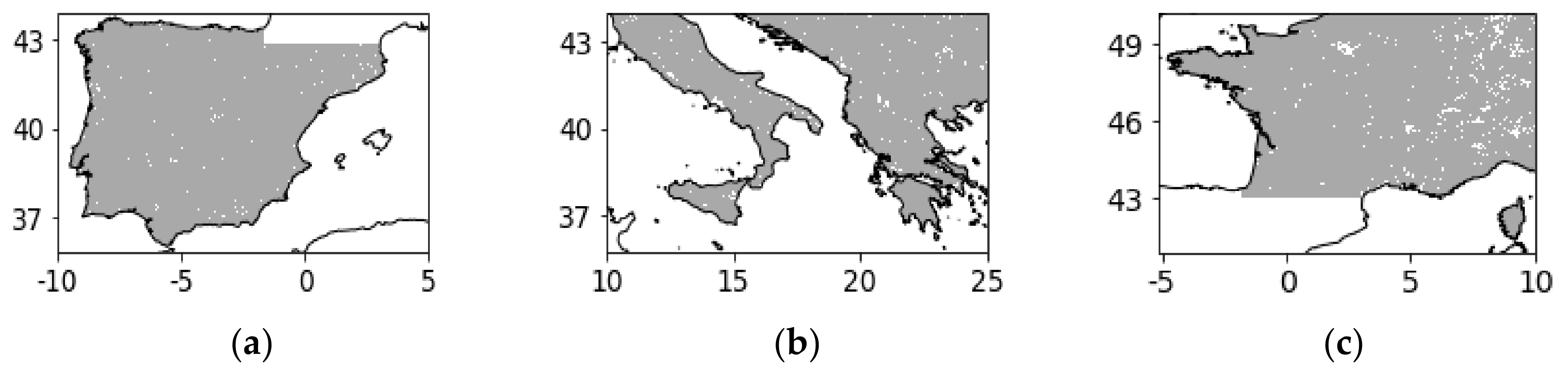
Three different areas of the Mediterranean basin were analysed separately to perform a deeper analysis of the behaviour of vegetation under extreme conditions. The study areas are represented in Figure 1.
The study areas are: Iberian Peninsula (hereafter IB, left panel); Eastern Mediterranean (hereafter EM, centre panel); and Western Europe (hereafter WE, right panel). The study period comprised the years between 2001 and 2019, which are covered by MODIS data.
2.2. Remote Sensing Data
2.2.1. Vegetation Productivity and Soil Moisture
Gross Primary Production (GPP) from MOD17A2 Collection 6 was used to monitor vegetation activity. As described in [37], in the MOD17 algorithm, GPP is calculated based on radiation conversion efficiency. This concept requires the estimation of the absorbed PAR (APAR), which in MOD17A2 relies on satellite-derived FPAR (Fraction of PAR) and IPAR (incident PAR) from MOD15 collection 6 and estimations of PAR provided by surface meteorological fields from GMAO/NASA. Also, information related to specific biome-type radiation-use efficiency is extracted from a biome properties look-up table to determine the radiation conversion efficiency parameter ε. GPP is then calculated as:
GPP = ε × (FPAR×IPAR) = ε × APAR
Collection 6 of MOD17A2 includes updates on global biome properties descriptions and meteorological inputs, as described in [38,39]. Various studies analysed the ability of MOD17A2 to reproduce the variability, both seasonal and interannual, across a broad range of different biomes; the results are quite accurate, especially in mid-latitudes, including the detection of hot and dry impacts on vegetation [18,38,39,40,41]. A detailed description of the product and algorithm can be found in [37]. The dataset is provided at 500 m spatial resolution on original projection (sinusoidal) and constitutes a daily cumulative composite of 8 days, expressed in kg C/m2/8days.
Soil water availability was monitored through the European Space Agency Climate Change Initiative Soil Moisture (ESA CCI SM, hereafter SM). The product has been recognized as a high-quality monitoring satellite product, useful for climate change and variability with meteorological and hydrological applications and land-atmosphere interaction studies [35,42,43,44,45]. In this work, the combined dataset, obtained from the combination of different active and passive datasets, is used with a spatial resolution of 0.25° and daily temporal resolution. It is described in volumetric units [m3m−3] and is representative of soil moisture in the top soil layer [35]. The detailed algorithm is described in [43]. The SM data were resampled to MODIS GPP resolution data for each study area by using the nearest neighbour interpolation scheme, as our main focus is to link the vegetation’s productivity disturbances in ecologically stressed areas to hot and dry events.
2.2.2. Land Surface Temperature
Land surface temperature was used in this study as a proxy of air temperature and was retrieved from MOD11A2 Collection 6 of the TERRA satellite [36]. The product consists of an 8-day composite, which corresponds to an average of daily daytime and night-time LST measurements over eight days, with 1 km of spatial resolution.
The determination of LST relies on the computation of surface emissivity, derived from two thermal infrared band channels (MODIS bands 31 and 32) [46]. The split-window algorithm also corrects atmospheric effects [47], using MODIS information about land cover types, clouds, snow, atmospheric water vapour and lower boundary air surface. More details related to the algorithm can be found in [36].
The latest MODIS LST version shows improvements related to adjustments on emissivity difference in bands 31 and 32 and several refinements of the split-window algorithm to compute LST of bare soil regions [36]. Moreover, [46] showed LST bias lower than 1 °C in the range of −10 to 58 °C. The low error values across this temperature range indicate the high accuracy and robustness of MODIS LST data to determine near-surface air temperature. The LST data were resampled to the resolution of GPP data (500 m) using the nearest neighbour interpolation scheme.
2.2.3. Land Cover
The University of Maryland global classification scheme (UMD) [48], available from the MODIS Land Cover Type Product (MCD12Q1) Collection 6, at a 500-metre spatial resolution and annual time step was used [49,50]. Land cover information was extracted only for the years considered as study cases.
UMD encompasses 17 different classes based on vegetation cover, the height of the canopy and the mosaics of cultivation [48]. The product has been widely used in different studies and the ultimate Collection 6 presents several refinements, both in the algorithm and resulting map datasets, that strongly improved the accuracy of land cover type detection [51].
2.3. Persistence of Vegetation Stress
This study follows an impact perspective, where the analysis is focused on ecological extreme responses [52]. Monthly anomaly fields of vegetation production (GPP) were computed per pixel as a departure from the monthly median of 2001–2019 and for each study area.
With the aim to identify the regions whose vegetation was under stress conditions, and following the methodology of [10,15], a monthly threshold of GPP was defined. The threshold was based on a pixel-by-pixel level and corresponds to −1 SD of monthly GPP. The ecologically stressed areas are thereby identified by the points which exhibit GPP anomalies under −1 SD during five or more months (out of twelve).
This approach accounts for differences in GPP variance across different eco-regions and between months [53], with the definition of “ecological extremes” likely associated with vegetation stress conditions [31]. It is worth mentioning that the applied methodology does not allow to distinguish between different drivers of low GPP. For example, burned areas cannot provide information on whether vegetation was under ecological stress. Therefore, burned pixels were masked in each study case through the FIRE CCI version 5.1. satellite product from ESA CCI, which maps the monthly burned areas at a 250-metre spatial resolution between 2001 and 2019 [54]. However, we cannot exclude that some pixels may be affected by other drivers, such as pests or diseases.
The methodology applied allowed for the selection of the extreme events which generated an extreme response by vegetation over the three study areas between 2001 and 2019 (Table 1).
2.4. Vegetation Productivity Losses
The assessment of impacts on vegetation productivity was performed by means of the annual accumulation of monthly GPP values over the considered affected area for the selected episodes (Table 1). The monthly cumulative GPP values for each event were compared with the historical median and the 25–75% variability range of affected pixels. The process was repeated annually, allowing to evaluate the functional recovery of vegetation productivity following a given extreme event.
For the year of the ecological extremes and the two subsequent years, spatial averages of monthly anomalies were determined in the affected pixels, as well as the annual productivity balance relative to the median. The end of the ecological extreme is defined as the moment when the values of GPP reached the historical median values. This analysis follows the perspective of [55] and provides an observation of functional productivity recovery over-stressed vegetation.
SM and LST monthly fields were used by computing, for each point, the monthly mean value to further study the dynamics of the relationships between vegetation productivity, soil moisture and land surface temperature over the stressed pixels. Monthly anomalies of LST and SM were also determined per pixel, as a departure from the monthly median of respective variables between 2001 and 2019, and for each study area.
The analysis of the influence of SM and LST on vegetation productivity was performed through the computation of spatial averaged seasonal cycles of pairs GPP–SM and GPP–LST and were compared with the corresponding monthly median cycle of each variable. Also, the relationships of GPP with both SM and LST over the stressed pixels for different types of vegetation were assessed through the computation of Pearson correlations between the correspondent anomalies of the variables.
2.5. Impacts on Land Cover
The 17 classes of UMD datasets were grouped into four main land cover types: high tree cover, low tree cover, cropland and others. High tree cover includes the classes correspondent to evergreen and deciduous broad-leaved, needle-leaved, mixed forests and woody savannas which are characterized by 30–60% of tree cover. Low tree cover is composed of mixed shrublands, grasslands and areas with 10–30% of tree cover. Cropland pixels comprise mosaics with more than 40% of cultivation. The other minor sectors correspond to wetlands and urban and non-vegetated areas, whose contribution to the annual balance of productivity disturbances is residual. The coverage of these main land cover types in the studied regions in the years of the selected extreme episodes is shown in Table 2.
To analyse the role of land cover on ecological extremes, we estimated spring and summer GPP anomalies for each land cover type and the corresponding annual productivity losses in order to assess the spatio-temporal variability of different land covers and characterize their ecological response to the extreme event.
3. Results
3.1. Ecological Extreme Detection
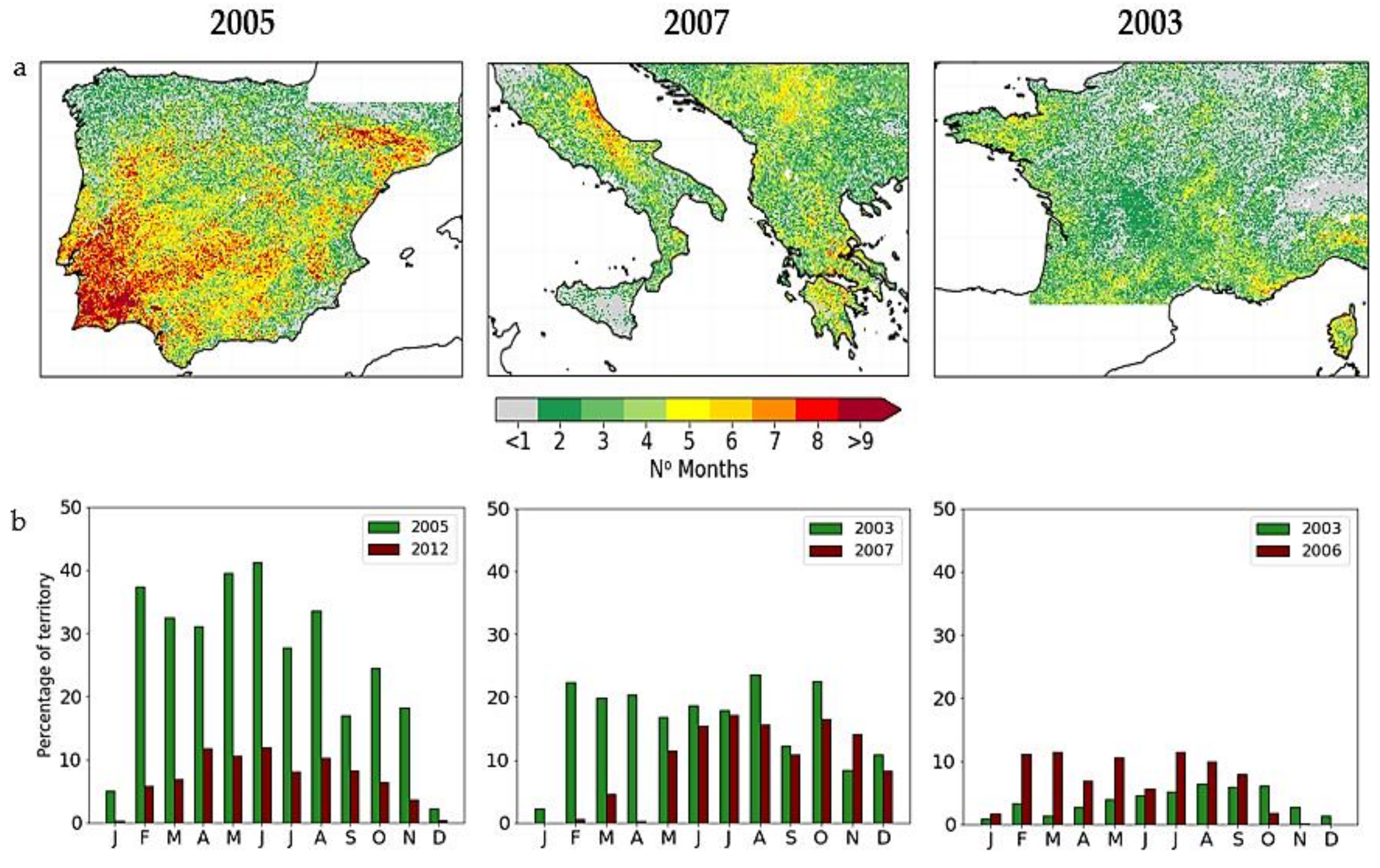
Figure 2 shows the number of months under stress, defined by GPP anomalies, for the studied cases of 2005 in IB, 2007 in EM and 2003 in WE, whose vegetation had more widespread extreme ecological stress. The percentage of territory with GPP anomalies below the specific pixel-level threshold was also analysed on a monthly basis. The results related to the studied cases of 2012 in IB, 2003 in EM and 2006 in WE are represented in Appendix A, Figure A1.
Spatial patterns of LST and SM anomaly values between March and September for the three different studied areas were performed and shown in Supplementary Material, (studied cases in IB), (studied cases in EM) and (study cases in WE).
During the 2005 episode, 250,655 km2 of IB vegetation was under ecological stress conditions for five or more months (out of 12) (Table 2), especially during the spring and summer, when more than 30% of Iberian ecosystems revealed productivity anomalies lower than the specific pixel-based threshold (Figure 2b, left panel, green bars). Vegetation stress was particularly prolonged in the south-western, western, and north-eastern territories, lasting up to 6–8 months (Figure 2a, left panel). These affected areas recorded high LST anomalies of about 3–5 °C and strong soil moisture deficits, especially between April and June. In the 2012 episode, the ecosystems of the north-east and south regions of IB were disturbed (Figure A1, left panel) and the vegetation seemed to be more affected between April and June (Figure 2b, left panel, red bars), coinciding with periods of strong LST anomalies, both negative (in April) and positive (in May and June), as well as strong soil moisture deficits.
Over EM, vegetative stress prevailed for five to seven months in 2003 in Italian and western Greece ecosystems (Figure A1, central panel), with high LST values being recorded over these regions especially in May and June. In 2007, stress conditions lasted five or more months on Italian and Greek territories (Figure 2a, central panel), affecting 76 112 km2, with more incidences during May, June and particularly in July (Figure 2b, central panel, red bars). During these months, the negative GPP anomalies recorded coincided with high temperatures (LST anomalies higher than 2–3 °C) and soil moisture deficits lower than −0.02 m3/m3.
In the WE domain, we found reductions in GPP for 5–7 months over 45 626 km2 in 2003 (Table 2), located around Southern France and Corsica (Figure 2a, top right panel). High LST anomalies were also found across the affected areas, with higher incidences between June and August. In 2006, 76 766 km2 of the vegetation of the WE region showed GPP anomalies lower than the specific monthly threshold during the spring and summer, especially in central and western areas of France (Figure A1, right panel), covering more than 10% of the study region (Figure 2b, right panel, red bars).
3.2. Seasonal Productivity Disturbances
Seasonal Impacts
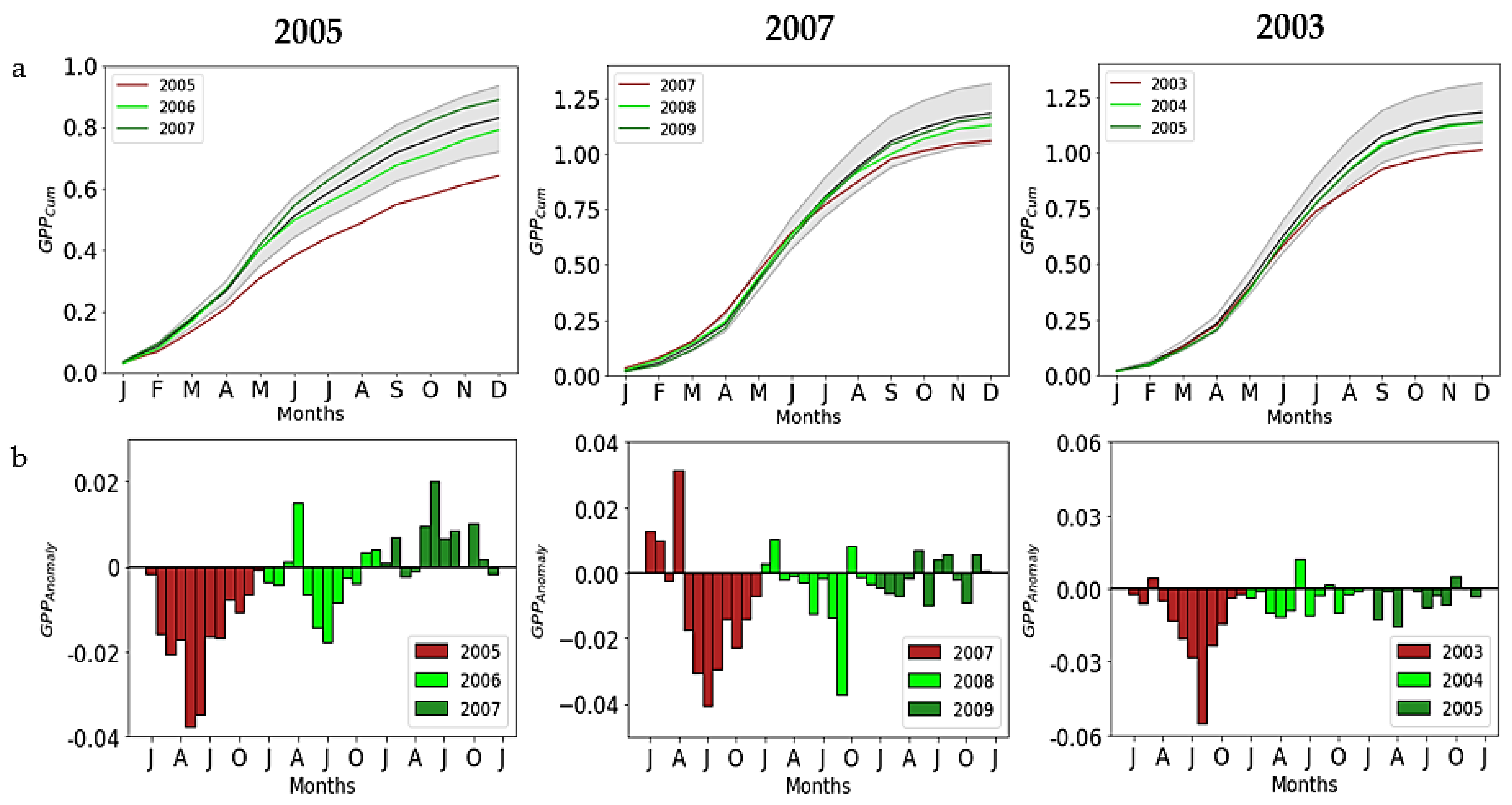
Reductions in gross productivity caused by the events of 2005 in IB, 2007 in EM and 2003 in WE are depicted in Figure 3. Related to the other study cases, the same information is represented in Figure A2. The annual productivity balance, computed for the stressed vegetation during each of the analysed extreme events and the two following years, is described in Table 3.
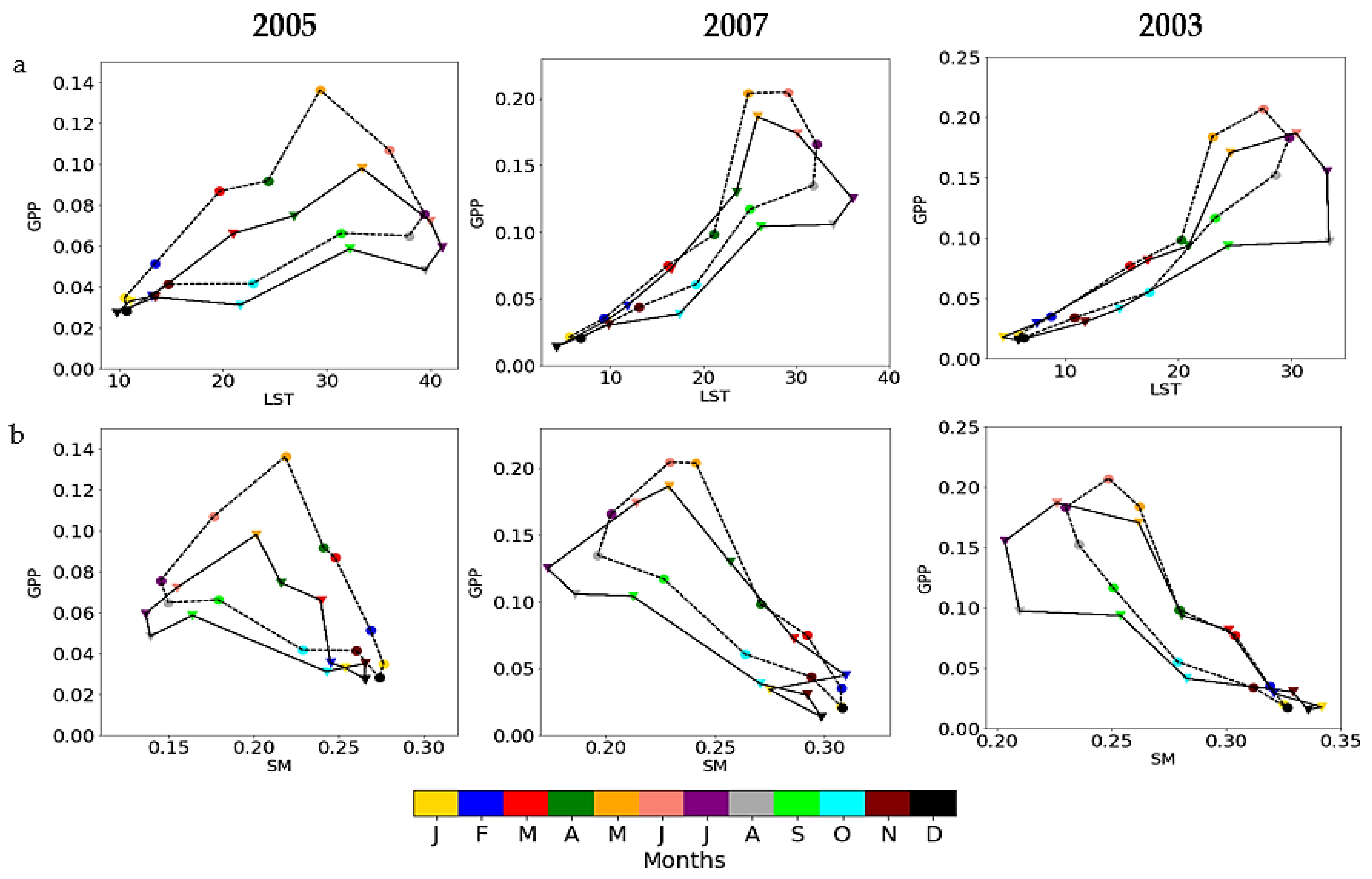
The relationships between GPP and SM and between GPP and LST during the extreme event year, are depicted in Figure 4 for the extreme events of 2005 in IB, 2007 in EM and 2003 in WE. The same results are illustrated in Figure A3 for the study cases of 2012 in IB, 2003 in EM and 2006 in WE.
In IB, the values of cumulative GPP across the stressed pixels during 2005 were below the 25–75% variability range (Figure 3a, top panel). GPP started departing from the long-term 25% tile during the winter months, which coincided with a departure of SM from the long-term median during these months (Figure 4b, left panel). The soil moisture stress was exacerbated in the spring, presenting high deficits from March to May, contributing to the reduction in GPP that reached anomalies nearly −0.04 kg C/m2/month in May and June. LST values above the historical median were also registered during this period (Figure 4a, left panel) and were stronger during the summer months, reaching more than +3 °C compared with the historical median in July and August. The disturbances of GPP, mainly caused by soil water stress and high temperatures, induced noticeable annual losses of productivity that reached a departure of ~47 TgC/year from historical median values (Table 3).
After 2005, cumulative annual productivity remained below average but within the 25–75% range in 2006 and registered above-average values in 2007 (Figure 3a,b, left panels, respectively). However, the disturbances were not compensated by the high activity of vegetation in 2007, as the balance of the three-year period (2005–2007) showed a remarkable GPP departure from the median of around −41 TgC/year (Table 3).
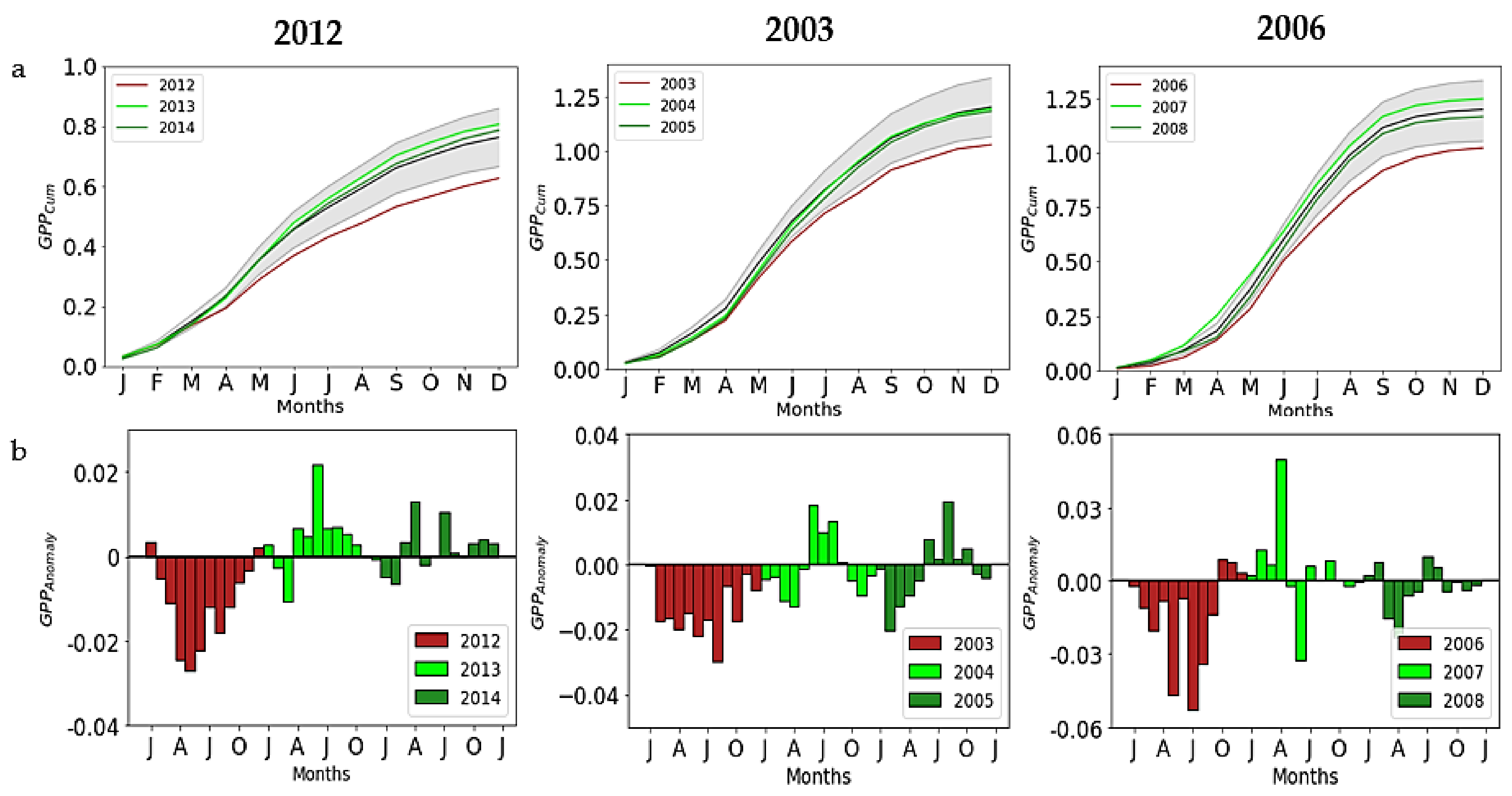
The results of the 2012 episode describe GPP cumulative values below the 25th percentile of affected pixels, mainly due to the productivity deficits which occurred during the spring and early summer (Figure A2, left panel). The seasonal cycle of the pair {SM–GPP} describes remarkable SM deficits of more than −0.05 m3/m3 in February and March (Figure A3, left panel) and large stress conditions on vegetation in April, May and June, as reflected in negative GPP anomalies (~−0.025 kg C/m2/month), described in Figure A2 (left panel).
In EM, the impacts of the 2003 episode on vegetation are expressed in a monthly cumulative GPP below the 25–75% variability range of affected pixels from March/April until the end of the year (Figure A2, central panel). SM deficits occurred during late winter and early spring, whereas LST values were higher than the historical median (about +3 °C) in May and June (Figure A3, central panel), resulting in a productivity decrease in the spring and amplified in the summer months. Negative GPP average anomalies reached about −0.03 kg C/m2/month in JJA (Figure A2, central panel), contributing to a large annual productivity loss of −21.12 TgC/year. GPP started to recover in the subsequent months, as shown by the annual accumulations of GPP close to the historical median in 2004 and 2005 (Figure A2, central panel).
The 2007 extreme event differs from the 2003 one in that the take-off of the negative anomalies at the regional scale occurred only during late spring, and the previous spring months are characterized by a monthly cumulative GPP above the long-term 75% tile and average anomalies reaching +0.032 kg C/m2/month in April (Figure 3a,b, central panels). This is reverted from May-onwards, with high LST values especially recorded in July and August, in conjunction with a rapid decrease in soil moisture content, which led to reductions in vegetation productivity (Figure 4a,b, central panel) that reached a low GPP anomaly in July (−0.041 kg C/m2/month). In the two years following 2007, large-scale recovery was only partial, as expressed by the consecutive months in spring and summer 2008 with negative GPP anomalies. Productivity in the affected vegetation was inhibited in subsequent months, as the annual balance of GPP between 2007 and 2009, over the affected pixels, reached a negative departure from the median of 14.10 TgC.
In WE, cumulative GPP changes in 2003 over the stressed pixels are characterized by two phases: one with values above the historical median until May and another, from June-onwards, with cumulative values below the 25th percentile (Figure 3a, right panel). High average LST anomalies were registered (+3.4 °C in July and +4.8 °C in August), accompanied by rapid reductions in soil moisture content in the summer (Figure 4a,b, right panel) resulting in strong monthly GPP anomalies, especially in July and August (Figure 3b, right panel).
The episode of 2003 was associated with vegetation losses over the affected pixels of −7.72 TgC/year; it is worth mentioning the inhibition of vegetation recovery over the following two years, as registered on negative GPP annual balances of −2.11 and −2.00 TgC/year in 2004 and 2005, respectively (Table 3).
For the 2006 episode, the cumulative GPP started to depart from the long-term 25–75% range in July, after several months with negative GPP anomalies (Figure A2, right panel). The strongest negative GPP anomalies were registered in the summer, concurrent with departures of SM from the long-term mean, as well as high LST values, especially in July (Figure A3, right panel). The recovery of soil moisture to normal values in the fall allowed for the recovery of GPP in the subsequent months. The annual disturbances of stressed vegetation were −13.58 TgC/year (Table 3), with the summer months representing the largest productivity deficits that occurred in that year.
3.3. Land Cover Response
The three study areas show distinct vegetation compositions. Low tree cover regions are the most abundant biome across IB and EM, representing, respectively, about 55% and 40% of the vegetation in the territories (Table 2). Conversely, in WE, croplands represent the main land cover type (Table 2) and had large reductions in GPP in 2003 and 2006.
We analysed the relationships between the anomalies in GPP, SM and LST in the spring and summer as well as the relationships between the anomalies of SM and LST for each land cover type (Tables S1, S2 and S3). In general, {SM–GPP} and {LST–GPP} showed opposite correlations in the spring (positive for SM–GPP and negative for LST–GPP), with few exceptions. In summer, the relationship between SM and GPP anomalies was generally positive, while LST and GPP anomalies were negatively correlated. During summer, correlation values were stronger for LST–GPP than for SM–GPP. Regarding the SM and LST anomalies relationship, a negative correlation was generally found.
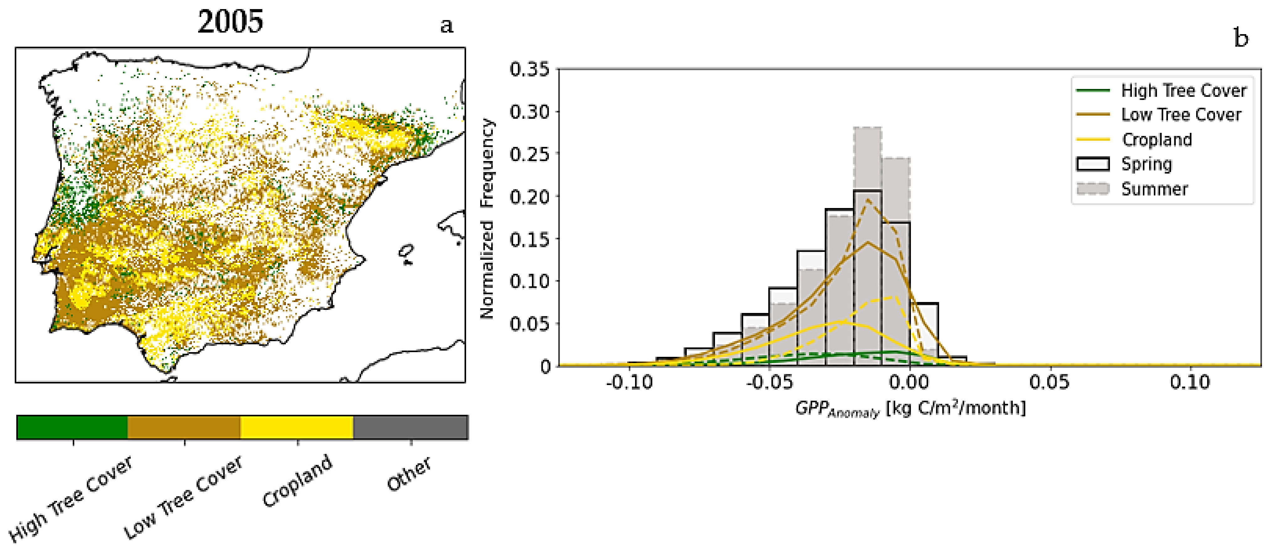
Results in Figure 5 indicate that in IB, croplands and low tree cover areas, which are mainly characterized by herbaceous vegetation, showed rapid reductions in productivity in the spring, with prolonged negative GPP anomalies which were further amplified in the summer months. On the other hand, high tree cover areas showed later reductions in productivity, with negative GPP anomalies occurring mainly in summer. This pattern is found in 2005 and 2012 in IB and 2003 in EM, where low tree cover areas represented the major contribution to the annual productivity balance of ecologically stressed vegetation (Table 4).
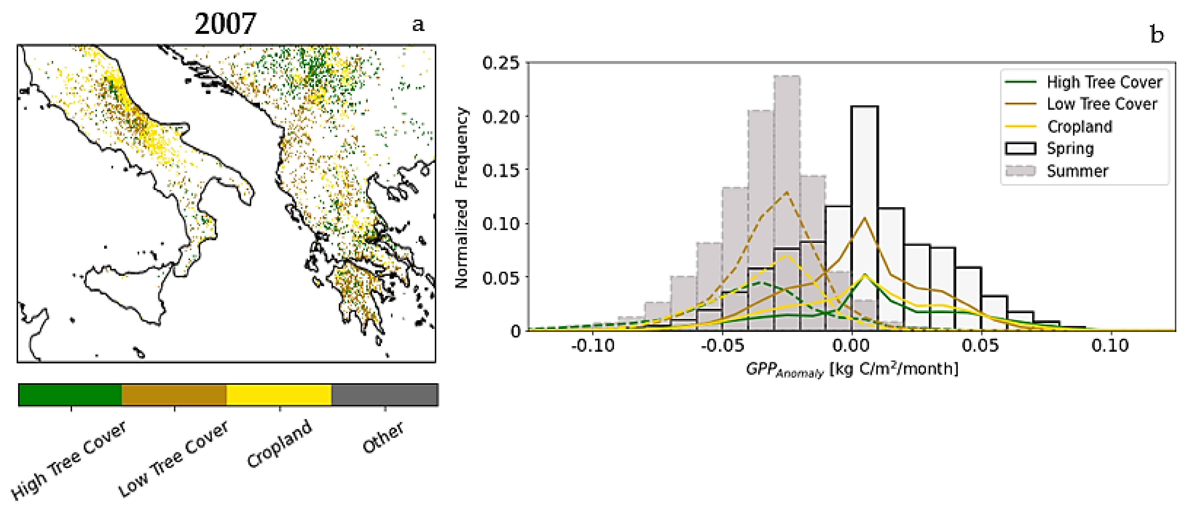
In contrast, the episodes of 2007 in EM (Figure 6) and 2003 (Figure 7) and 2006 in WE showed distinct responses of the different land cover types to temperature and SM anomalies in the spring and summer. The increase of hot and dry conditions in the summer months resulted in a strong reduction of productivity of all land covers, as represented in the shift to lower values of GPP anomalies.
It is worth mentioning that, despite their higher abundance across EM and WE, high tree cover areas seemed to have a higher reduction in GPP compared with the study cases of IB, as described with the prolonged frequency of this land cover type to the lowest GPP anomalies in summer (below −0.05 kg C/m2/month) (Figure 6b and Figure 7b).
4. Discussion
The European part of the Mediterranean basin is a climate change hotspot for droughts, heatwaves [1,8] and other extreme events. Several studies have identified a high risk for increased water stress on crops and natural ecosystems over a broader area of the southern sectors of Europe, the Mediterranean, the Middle East and North Africa [56,57]. We analysed the ecological response to the occurrence of hot and dry events in the European part of the Mediterranean basin’s vegetation productivity, with particular emphasis on the most severe episodes that occurred in the Iberian Peninsula, Eastern Mediterranean and Western Europe between 2001 and 2019.
Our results showed that the episodes which occurred in the Iberian Peninsula in 2005 and 2012 led to an extreme ecological response from the vegetation. The land cover of this region is quite adapted to water-limited conditions, especially in summer [58]. However, [10,12] we were able to pinpoint that the 2005 drought in IB started in the fall of 2004 and [59] traced the take-off of the 2012 drought back to the fall/winter of 2011. Therefore, the cumulative effect of persistent drought for several months might have driven vegetation to consecutive productivity deficits, agreeing with [60,61] that highlighted the dependence of vegetation on water availability in IB. On the other hand, the comparison between the correlations of SM–GPP, LST–GPP and also SM–LST anomalies, across all land cover types during summer, suggested that high LST anomalies played an important role in the amplification of ecological stress in 2005, not only due to the strong effect of high summer temperatures on soil moisture depletion but also possibly due to a direct negative effect of heat stress (from high LST) on GPP. The coupling of SM and LST verified that soil moisture–temperature feedback has a clear influence on vegetation, as clearly pointed out by [24].
We have shown in the IB studied cases that productivity in croplands and low tree cover areas is reduced more rapidly in response to dry spring conditions, while high tree cover areas showed negative GPP anomalies later, in summer. These results agree with [62,63], who observed that in water-limited environments, forests tend to develop deeper roots, which may allow them to access deeper soil water, increasing their resistance to short-term drought.
A point that should be elevated here is related to the intra-seasonal variability of GPP. In IB, the negative correlation between LST-GPP anomalies and positive correlation between SM–GPP anomalies, both in the spring, indicated an already a water-limited regime in this season, which is consistent with the prolonged drought situations. In the IB 2012 episode, a negative correlation between SM–GPP in the spring was found in high tree cover areas, contrary to the other land cover types that showed weak SM–GPP and LST–GPP relationships (Table S1). The negative correlation can be possibly linked to the strong negative temperature anomalies (−5 °C) in April in high forest cover areas. These results may be linked to spring frost at night which could result in leaf or bud damage during the early growing season and may affect vegetation productivity throughout the year [64].
The results of the Eastern Mediterranean and Western Europe studied cases found an amplification of the GPP anomalies during the summer. The exacerbation of negative GPP may be linked to compounding hot and dry summer conditions. For instance, in WE, the large GPP anomalies were associated with summer heatwaves, both during 2003 [18,65,66] and 2006 [67]. Moreover, the correlation results in 2006 may suggest the concurrency of hot and dry conditions in the summer, caused by the July heatwave [67] and the soil moisture depletion, which led to strong reductions in GPP anomalies. These results in EM and WE enhance the influence of heat-drought coupling on vegetation productivity.
An important aspect that should be stressed is the link between spring conditions and hot summers. Warm springs trigger earlier vegetation activity and may contribute to reducing the soil water availability in the summer [20,68] and [69] showed that warm springs can amplify summer temperatures. Our results in EM in 2007 are consistent with this effect: vegetation activity until April was higher than normal, associated with high spring temperatures and dry conditions which started in late spring, which, along with extreme hot summer conditions, may have exacerbated the reduction in soil water availability and driven the vegetation to critical ecological stress in several areas of the Eastern Mediterranean.
Our results have highlighted the important role of hot and dry events in vegetation productivity. Nevertheless, some key points were not addressed here, related to the high heterogeneity of the Mediterranean basin in terms of land use changes, soil properties, topography and land management policies [70], which can partly affect the results of different land cover responses to heat and drought. Another aspect that was not addressed was the vegetation memory effect, as we used only remote sensing data and our analysis showed the vegetation productivity recovery before the next ecological event. This can be accommodated through the application of approaches that are able to incorporate vegetation memory (e.g., through the use of ARx models [71,72]). These models allowed for a better quantification and understanding of hot and dry effects on vegetation productivity [73]. Finally, our study period comprised 19 years (2001–2019), relying on the availability of MODIS satellite data, which can constitute a limitation to the assessment of extreme events on vegetation since a climatic long-term dataset calls for an extended period of 30 years. Although this study presents the referred limitations, we firmly believe that the proposed approach is highly valuable and can be easily replicated to other areas. Moreover, this approach will surely be useful, supplying responsible authorities and managers with a spatially comprehensive tool aiming for the development of mitigation plans that will be crucial in the case of the occurrence of more frequent hot and dry episodes.
5. Conclusions
Here, we analysed a set of extreme ecological events between 2001 and 2019 in the Mediterranean region and assessed how they are related to soil moisture and land surface temperature. We selected the two most severe episodes from each of the three domains and evaluated GPP over the affected areas in the year of extreme events and the two subsequent years.
Our results show the influence of the land–atmosphere coupling on Mediterranean vegetation, with soil moisture–temperature feedbacks playing an important role in vegetation productivity, as well as the importance of warm springs in contributing to early soil moisture depletion and the amplification of hot and dry summer impacts on vegetation. High tree cover areas showed generally higher resistance to dry conditions than low tree cover areas and croplands.
Our work highlights how remote sensing data can be used to detect and monitor ecological extremes, their functional recovery times and the role of land cover in mediating these relationships. Furthermore, the projected increase in the frequency and severity of hot and dry conditions in the Mediterranean emphasizes the need for understanding the dynamics of their impact on vegetation and recovery times in this region.
Supplementary Materials
Table S1, Table S2, Table S3 Pearson correlation coefficients between SM-GPP, LST-GPP and SM_LST anomalies during spring and summer for each land cover-type in 2005 and 2012 over IB; The following are available online at https://0-www-mdpi-com.brum.beds.ac.uk/article/10.3390/rs13194010/s1, Tables S1, S2, S3.
Author Contributions
T.E., A.C.R. and C.M.G. participated in the conceptual design of the study. All the authors contributed to the interpretation and analysis of the results and the redaction of the manuscript. C.M.G., A.B. and A.C.R. defined the datasets and the methodology to be used for the study. T.E. made all the calculations, figures and tables and wrote the manuscript. Each of the co-authors performed a thorough revision of the manuscript, provided useful advice on the intellectual content and improved the English language. All authors have read and agreed to the published version of the manuscript.
Funding
This work was partially supported by national funds through FCT (Fundação para a Ciência e Tecnologia, Portugal) through projects IMPECAF (PTDC/CTA–CLI/28902/2017), FireCast (PCIF/GRF/0204/2017) and UIBD/50019/2020–Instituto Dom Luiz.
Institutional Review Board Statement
Not applicable.
Informed Consent Statement
Not applicable.
Data Availability Statement
Not applicable.
Conflicts of Interest
The authors declare no conflict of interest.
Appendix A
Figure A1.
As in Figure 2, but over IB during 2012 event (left panels), EM during 2003 event (central panels) and WE during 2006 event (right panels).
Figure A1.
As in Figure 2, but over IB during 2012 event (left panels), EM during 2003 event (central panels) and WE during 2006 event (right panels).

Figure A2.
As in Figure 3 but over IB during 2012 event (left panels), EM during 2003 event (central panels) and WE during 2006 event (right panels).
Figure A2.
As in Figure 3 but over IB during 2012 event (left panels), EM during 2003 event (central panels) and WE during 2006 event (right panels).

Figure A3.
As in Figure 4 but over IB during 2012 event (left panels), EM during 2003 event (central panels) and WE during 2006 event (right panels).
Figure A3.
As in Figure 4 but over IB during 2012 event (left panels), EM during 2003 event (central panels) and WE during 2006 event (right panels).

References
- IPCC. Global Warming of 1.5 °C; IPCC: Geneva, Switzerland, 2018. [Google Scholar]
- Melillo, J.M.; McGuire, A.D.; Kicklighter, D.W.; Moore, B.; Vorosmarty, C.J.; Schloss, A.L. Global climate change and terrestrial net primary production. Nature 1993, 363, 234–240. [Google Scholar] [CrossRef]
- Ruffault, J.; Curt, T.; Martin-StPaul, N.K.; Moron, V.; Trigo, R.M. Extreme wildfire events are linked to global-change-type droughts in the northern Mediterranean. Nat. Hazards Earth Syst. Sci. 2018, 18, 847–856. [Google Scholar] [CrossRef] [Green Version]
- Zscheischler, J.; Mahecha, M.D.; von Buttlar, J.; Harmeling, S.; Jung, M.; Rammig, A.; Randerson, J.T.; Schölkopf, B.; Seneviratne, S.I.; Tomelleri, E. A few extreme events dominate global interannual variability in gross primary production. Environ. Res. Lett. 2014, 9, 035001. [Google Scholar] [CrossRef] [Green Version]
- Ciais, P.; Reichstein, M.; Viovy, N.; Granier, A.; Ogee, J.; Allard, V.; Aubinet, M.; Buchmann, N.; Bernhofer, C.; Carrara, A.; et al. Europe-wide reduction in primary productivity caused by the heat and drought in 2003. Nature 2005, 437, 529–533. [Google Scholar] [CrossRef] [PubMed]
- Flach, M.; Sippel, S.; Gans, F.; Bastos, A.; Brenning, A.; Reichstein, M.; Mahecha, M.D. Contrasting biosphere responses to hydrometeorological extremes: Revisiting the 2010 western Russian heatwave. Biogeosciences 2018, 15, 6067–6085. [Google Scholar] [CrossRef] [Green Version]
- Grillakis, M.G. Increase in severe and extreme soil moisture droughts for Europe under climate change. Sci. Total. Environ. 2019, 660, 1245–1255. [Google Scholar] [CrossRef] [PubMed]
- Spinoni, J.; Vogt, J.V.; Naumann, G.; Barbosa, P.; Dosio, A. Will drought events become more frequent and severe in Europe? Int. J. CLimatol. 2018, 38, 1718–1736. [Google Scholar] [CrossRef] [Green Version]
- Orlowsky, B.; Seneviratne, S.I. Elusive drought: Uncertainty in observed trends and short- and long-term CMIP5 projections. Hydrol. Earth Syst. Sci. 2013, 17, 1765–1781. [Google Scholar] [CrossRef] [Green Version]
- Gouveia, C.; Trigo, R.; DaCamara, C. Drought and vegetation stress monitoring in Portugal using satellite data. Nat. Hazards Earth Syst. Sci. 2009, 9, 185–195. [Google Scholar] [CrossRef] [Green Version]
- Gouveia, C.; Bastos, A.; Trigo, R.; DaCamara, C. Drought impacts on vegetation in the pre- and post-fire events over Iberian Peninsula. Nat. Hazards Earth Syst. Sci. 2012, 12, 3123–3137. [Google Scholar] [CrossRef]
- García-Herrera, R.; Paredes, D.; Trigo, R.M.; Trigo, I.F.; Hernández, E.; Barriopedro, D.; Mendes, M.A. The outstanding 2004/05 drought in the Iberian Peninsula: Associated atmospheric circulation. J. Hydrometeorol. 2007, 8, 483–498. [Google Scholar] [CrossRef] [Green Version]
- Sánchez-Benítez, A.; García-Herrera, R.; Barriopedro, D.; Sousa, P.M.; Trigo, R.M. June 2017: The Earliest European Summer Mega-heatwave of Reanalysis Period. Geophys. Res. Lett. 2018, 45, 1955–1962. [Google Scholar] [CrossRef]
- Turco, M.; Jerez, S.; Augusto, S.; Tarín-Carrasco, P.; Ratola, N.; Jiménez-Guerrero, P.; Trigo, R. Climate drivers of the 2017 devastating fires in Portugal. Sci. Rep. 2019, 9, 13886. [Google Scholar] [CrossRef]
- Gouveia, C.M.; Bistinas, I.; Liberato, M.; Bastos, A.; Koutsias, N.; Trigo, R. The outstanding synergy between drought, heatwaves and fuel on the 2007 Southern Greece exceptional fire season. Agric. For. Meteorol. 2016, 218-219, 135–145. [Google Scholar] [CrossRef]
- Koutsias, N.; Arianoutsou, M.; Kallimanis, A.S.; Mallinis, G.; Halley, J.M.; Dimopoulos, P. Where did the fires burn in Peloponnisos, Greece the summer of 2007? Evidence for a synergy of fuel and weather. Agric. For. Meteorol. 2012, 156, 41–53. [Google Scholar] [CrossRef]
- Tolika, K.; Maheras, P.; Tegoulias, I. Extreme temperatures in Greece during 2007: Could this be a “return to the future”? Geophys. Res. Lett. 2009, 36, L10813. [Google Scholar] [CrossRef]
- Bastos, A.; Gouveia, C.M.; Trigo, R.M.; Running, S.W. Analysing the spatio-temporal impacts of the 2003 and 2010 extreme heatwaves on plant productivity in Europe. Biogeosciences 2014, 11, 3421–3435. [Google Scholar] [CrossRef] [Green Version]
- Rodriguez-Iturbe, I.; D’Odorico, P.; Porporato, A.; Ridolfi, L. On the spatial and temporal links between vegetation, climate, and soil moisture. Water Resour. Res. 1999, 35, 3709–3722. [Google Scholar] [CrossRef]
- Bastos, A.; Ciais, P.; Friedlingstein, P.; Sitch, S.; Pongratz, J.; Fan, L.; Wigneron, J.P.; Weber, U.; Reichstein, M.; Fu, Z.; et al. Direct and seasonal legacy effects of the 2018 heat wave and drought on European ecosystem productivity. Sci. Adv. 2020, 6, eaba2724. [Google Scholar] [CrossRef] [PubMed]
- Fischer, E.M.; Seneviratne, S.; Vidale, P.L.; Lüthi, D.; Schär, C. Soil Moisture–Atmosphere Interactions during the 2003 European Summer Heat Wave. J. Clim. 2007, 20, 5081–5099. [Google Scholar] [CrossRef]
- Whan, K.; Zscheischler, J.; Orth, R.; Shongwe, M.; Rahimi, M.; Asare, E.O.; Seneviratne, S. Impact of soil moisture on extreme maximum temperatures in Europe. Weather. Clim. Extremes 2015, 9, 57–67. [Google Scholar] [CrossRef] [Green Version]
- Hirschi, M.; Seneviratne, S.; Alexandrov, V.; Boberg, F.; Boroneant, C.; Christensen, O.B.; Formayer, H.; Orlowsky, B.; Stepanek, P. Observational evidence for soil-moisture impact on hot extremes in southeastern Europe. Nat. Geosci. 2010, 4, 17–21. [Google Scholar] [CrossRef]
- Seneviratne, S.I.; Corti, T.; Davin, E.L.; Hirschi, M.; Jaeger, E.B.; Lehner, I.; Orlowsky, B.; Teuling, A.J. Investigating soil moisture-climate interactions in a climate change: A review. Earth Sci. Rev. 2010, 99, 125–161. [Google Scholar] [CrossRef]
- Seneviratne, S.I.; Wilhelm, M.; Stanelle, T.; Hurk, B.V.D.; Hagemann, S.; Berg, A.; Cheruy, F.; Higgins, M.E.; Meier, A.; Brovkin, V.; et al. Impact of soil moisture-climate feedbacks on CMIP5 projections: First results from the GLACE-CMIP5 experiment. Geophys. Res. Lett. 2013, 40, 5212–5217. [Google Scholar] [CrossRef] [Green Version]
- Vogel, M.M.; Orth, R.; Cheruy, F.; Hagemann, S.; Lorenz, R.; Hurk, B.J.J.M.V.D.; Seneviratne, S.I. Regional amplification of projected changes in extreme temperatures strongly controlled by soil moisture-temperature feedbacks. Geophys. Res. Lett. 2017, 44, 1511–1519. [Google Scholar] [CrossRef]
- Vicente-Serrano, S.M.; McVicar, T.R.; Miralles, D.; Yang, Y.; Tomas-Burguera, M. Unraveling the influence of atmospheric evaporative demand on drought and its response to climate change. Wiley Interdiscip. Rev. Clim. Chang. 2019, 11, e632. [Google Scholar] [CrossRef]
- Ballantyne, A.; Smith, W.; Anderegg, W.; Kauppi, P.; Sarmiento, J.; Tans, P.; Shevliakova, E.; Pan, Y.; Poulter, B.; Anav, A.; et al. Accelerating net terrestrial carbon uptake during the warming hiatus due to reduced respiration. Nat. Clim. Chang. 2017, 7, 148–152. [Google Scholar] [CrossRef]
- Turco, M.; Von Hardenberg, J.; AghaKouchak, A.; Llasat, M.C.; Provenzale, A.; Trigo, R. On the key role of droughts in the dynamics of summer fires in Mediterranean Europe. Sci. Rep. 2017, 7, 1–10. [Google Scholar] [CrossRef] [Green Version]
- Rouault, G.; Candau, J.-N.; Lieutier, F.; Nageleisen, L.-M.; Martin, J.-C.; Warzée, N. Effects of drought and heat on forest insect populations in relation to the 2003 drought in Western Europe. Ann. For. Sci. 2006, 63, 613–624. [Google Scholar] [CrossRef]
- Smith, M.D. An ecological perspective on extreme climatic events: A synthetic definition and framework to guide future research. J. Ecol. 2011, 99, 656–663. [Google Scholar] [CrossRef]
- Frank, D.; Reichstein, M.; Bahn, M.; Thonicke, K.; Frank David Mahecha, M.D.; Smith, P.; van der Velde, M.; Vicca, S.; Babst, F.; Beer, C.; et al. Effects of climate extremes on the terrestrial carbon cycle: Concepts, processes and potential future impacts. Glob. Chang. Biol. 2015, 21, 2861–2880. [Google Scholar] [CrossRef] [Green Version]
- Peters, W.; Bastos, A.; Ciais, P.; Vermeulen, A. A historical, geographical and ecological perspective on the 2018 European summer drought. Philos. Trans. R. Soc. B Biol. Sci. 2020, 375, 20190505. [Google Scholar] [CrossRef] [PubMed]
- Teuling, A.; Seneviratne, S.; Stöckli, R.; Reichstein, M.; Moors, E.; Ciais, P.; Luyssaert, S.; Hurk, B.V.D.; Ammann, C.; Bernhofer, C.; et al. Contrasting response of European forest and grassland energy exchange to heatwaves. Nat. Geosci. 2010, 3, 722–727. [Google Scholar] [CrossRef]
- Dorigo, W.; De Jeu, R.; Chung, D.; Parinussa, R.; Liu, Y.; Wagner, W.; Fernández-Prieto, D. Evaluating global trends (1988-2010) in harmonized multi-satellite surface soil moisture. Geophys. Res. Lett. 2012, 39, L18405. [Google Scholar] [CrossRef] [Green Version]
- Wan, Z. New refinements and validation of the collection-6 MODIS land-surface temperature/emissivity product. Remote. Sens. Environ. 2014, 140, 36–45. [Google Scholar] [CrossRef]
- Running, S.W.; Nemani, R.R.; Heinsch, F.A.; Zhao, M.; Reeves, M.; Hashimoto, H. A Continuous Satellite-Derived Measure of Global Terrestrial Primary Production. BioScience 2004, 54, 547–560. [Google Scholar] [CrossRef]
- Zhao, M.; Heinsch, F.A.; Nemani, R.R.; Running, S.W. Improvements of the MODIS terrestrial gross and net primary production global data set. Remote. Sens. Environ. 2005, 95, 164–176. [Google Scholar] [CrossRef]
- Zhao, M.; Running, S.W.; Nemani, R.R. Sensitivity of Moderate Resolution Imaging Spectroradiometer (MODIS) terrestrial primary production to the accuracy of meteorological reanalyses. J. Geophys. Res. Space Phys. 2006, 111, G01002. [Google Scholar] [CrossRef] [Green Version]
- Frazier, A.E.; Renschler, C.S.; Miles, S.B. Evaluating post-disaster ecosystem resilience using MODIS GPP data. Int. J. Appl. Earth Obs. Geoinf. 2013, 21, 43–52. [Google Scholar] [CrossRef]
- Reichstein, M.; Ciais, P.; Papale, D.; Valentini, R.; Running, S.; Viovy, N.; Cramer, W.; Granier, A.; Ogée, J.; Allard, V.; et al. Reduction of ecosystem productivity and respiration during the European summer 2003 climate anomaly: A joint flux tower, remote sensing and modelling analysis. Glob. Chang. Biol. 2006, 13, 634–651. [Google Scholar] [CrossRef]
- Dorigo, W.; Gruber, A.; De Jeu, R.; Wagner, W.; Stacke, T.; Loew, A.; Albergel, C.; Brocca, L.; Chung, D.; Parinussa, R.; et al. Evaluation of the ESA CCI soil moisture product using ground-based observations. Remote. Sens. Environ. 2014, 162, 380–395. [Google Scholar] [CrossRef]
- Dorigo, W.; Wagner, W.; Albergel, C.; Albrecht, F.; Balsamo, G.; Brocca, L.; Chung, D.; Ertl, M.; Forkel, M.; Gruber, A.; et al. ESA CCI Soil Moisture for improved Earth system understanding: State-of-the art and future directions. Remote. Sens. Environ. 2017, 203, 185–215. [Google Scholar] [CrossRef]
- Casagrande, E.; Mueller, B.; Miralles, D.G.; Entekhabi, D.; Molini, A. Wavelet correlations to reveal multiscale coupling in geophysical systems. J. Geophys. Res. Atmos. 2015, 120, 7555–7572. [Google Scholar] [CrossRef] [Green Version]
- Liu, Y.Y.; Parinussa, R.M.; Dorigo, W.A.; De Jeu, R.A.M.; Wagner, W.; van Dijk, A.I.J.M.; McCabe, M.F.; Evans, J.P. Developing an improved soil moisture dataset by blending passive and active microwave satellite-based retrievals. Hydrol. Earth Syst. Sci. 2011, 15, 425–436. [Google Scholar] [CrossRef] [Green Version]
- Wan, Z. New refinements and validation of the MODIS Land-Surface Temperature/Emissivity products. Remote. Sens. Environ. 2008, 112, 59–74. [Google Scholar] [CrossRef]
- Wan, Z.; Dozier, J. A generalized split-window algorithm for retrieving land-surface temperature from space. IEEE Trans. Geosci. Remote. Sens. 1996, 34, 892–905. [Google Scholar] [CrossRef] [Green Version]
- Hansen, M.C.; DeFries, R.S.; Townshend, J.R.G.; Sohlberg, R.A. Global land cover classification at 1 km spatial resolution using a classification tree approach. Int. J. Remote. Sens. 2000, 21, 1331–1364. [Google Scholar] [CrossRef]
- Friedl, M.; McIver, D.; Hodges, J.; Zhang, X.; Muchoney, D.; Strahler, A.; Woodcock, C.; Gopal, S.; Schneider, A.; Cooper, A.; et al. Global land cover mapping from MODIS: Algorithms and early results. Remote. Sens. Environ. 2002, 83, 287–302. [Google Scholar] [CrossRef]
- Friedl, M.A.; Sulla-Menashe, D.; Tan, B.; Schneider, A.; Ramankutty, N.; Sibley, A.; Huang, X. MODIS Collection 5 global land cover: Algorithm refinements and characterization of new datasets. Remote. Sens. Environ. 2010, 114, 168–182. [Google Scholar] [CrossRef]
- Sulla-Menashe, D.; Gray, J.M.; Abercrombie, S.P.; Friedl, M.A. Hierachical mapping of annual global land cover 2001 to present: The MODIS Collection 6 Land Cover Product. Remote. Sens. Environ. 2019, 222, 183–194. [Google Scholar] [CrossRef]
- Reichstein, M.; Bahn, M.; Ciais, P.; Frank, D.; Mahecha, M.D.; Seneviratne, S.I.; Zscheischler, J.; Beer, C.; Buchmann, N.; Frank, D.C.; et al. Climate extremes and the carbon cycle. Nature 2013, 500, 287–295. [Google Scholar] [CrossRef]
- Beer, C.; Reichstein, M.; Tomelleri, E.; Ciais, P.; Jung, M.; Carvalhais, N.; Rödenbeck, C.; Arain, M.A.; Baldocchi, D.; Bonan, G.B.; et al. Terrestrial Gross Carbon Dioxide Uptake: Global Distribution and Covariation with Climate. Science 2010, 329, 834–838. [Google Scholar] [CrossRef] [Green Version]
- Lizundia-Loiola, J.; Otón, G.; Ramo, R.; Chuvieco, E. A spatio-temporal active-fire clustering approach for global burned area mapping at 250 m from MODIS data. Remote. Sens. Environ. 2019, 236, 111493. [Google Scholar] [CrossRef]
- Cooper, L.A.; Ballantyne, A.P.; Holden, Z.A.; Landguth, E.L. Disturbance impacts on land surface temperature and gross primary productivity in the western United States. J. Geophys. Res. Biogeosci. 2017, 122, 930–946. [Google Scholar] [CrossRef]
- Gao, X.; Giorgi, F. Increased aridity in the Mediterranean region under greenhouse gas forcing estimated from high resolution simulations with a regional climate model. Glob. Planet. Chang. 2008, 62, 195–209. [Google Scholar] [CrossRef]
- Hoerling, M.P.; Eischeid, J.K.; Perlwitz, J.; Quan, X.; Zhang, T.; Pegion, P.J. On the Increased Frequency of Mediterranean Drought. J. Clim. 2012, 25, 2146–2161. [Google Scholar] [CrossRef] [Green Version]
- Gouveia, C.; Trigo, R.M.; DaCamara, C.; Libonati, R.; Pereira, J.M.C. The North Atlantic Oscillation and European vegetation dynamics. Int. J. Clim. 2008, 28, 1835–1847. [Google Scholar] [CrossRef]
- Trigo, R.M.; Añel, J.; Barriopedro, D.; García-Herrera, R.; Gimeno, L.; Nieto, R.; Castillo, R.; Allen, M.R.; Massey, N. The recorded winter drought of 2011-12 in the Iberian Peninsula. Bull. Amer. Meteorol. Soc. 2013, 94, S41–S45. [Google Scholar]
- Vicente-Serrano, S.M.; Heredia-Laclaustra, A. NAO influence on NDVI trends in the Iberian peninsula (1982–2000). Int. J. Remote. Sens. 2004, 25, 2871–2879. [Google Scholar] [CrossRef]
- Vicente-Serrano, S.M. Evaluating the Impact of Drought Using Remote Sensing in a Mediterranean, Semi-arid Region. Nat. Hazards 2006, 40, 173–208. [Google Scholar] [CrossRef]
- Zhou, G.; Wei, X.; Chen, X.; Zhou, P.; Liu, X.; Xiaohua, W.; Sun, G.; Scott, D.F.; Zhou, S.; Han, L.; et al. Global pattern for the effect of climate and land cover on water yield. Nat. Commun. 2015, 6, 5918. [Google Scholar] [CrossRef] [Green Version]
- Fan, Y.; Miguez-Macho, G.; Jobbágy, E.G.; Jackson, R.B.; Otero-Casal, C. Hydrologic regulation of plant rooting depth. Proc. Natl. Acad. Sci. USA 2017, 114, 10572–10577. [Google Scholar] [CrossRef] [PubMed] [Green Version]
- Bascietto, M.; Bajocco, S.; Ferrara, C.; Alivernini, A.; Santangelo, E. Estimating late spring frost-induced growth anomalies in European beech forests in Italy. Int. J. Biometeorol. 2019, 63, 1039–1049. [Google Scholar] [CrossRef] [PubMed]
- Herrera, R.F.G.; Díaz, J.; Trigo, R.; Luterbacher, J.; Fischer, E. A Review of the European Summer Heat Wave of 2003. Crit. Rev. Environ. Sci. Technol. 2010, 40, 267–306. [Google Scholar] [CrossRef]
- Trigo, R.M.; García-Herrera, R.; Díaz, J.; Trigo, I.F.; Valente, M.A. How exceptional was the early August 2003 heatwave in France? Geophys. Res. Lett. 2005, 32, L10701. [Google Scholar] [CrossRef] [Green Version]
- Rebetez, M.; Dupont, O.; Giroud, M. An analysis of the July 2006 heatwave extent in Europe compared to the record year of 2003. Theor. Appl. Clim. 2008, 95, 1–7. [Google Scholar] [CrossRef] [Green Version]
- Buermann, W.; Bikash, P.R.; Jung, M.; Burn, D.H.; Reichstein, M. Earlier springs decrease peak summer productivity in North American boreal forests. Environ. Res. Lett. 2013, 8, 024027. [Google Scholar] [CrossRef]
- Haslinger, K.; Blöschl, G. Space-Time Patterns of Meteorological Drought Events in the European Greater Alpine Region Over the Past 210 Years. Water Resour. Res. 2017, 53, 9807–9823. [Google Scholar] [CrossRef] [Green Version]
- Gouveia, C.; Trigo, R.; Beguería, S.; Vicente-Serrano, S. Drought impacts on vegetation activity in the Mediterranean region: An assessment using remote sensing data and multi-scale drought indicators. Glob. Planet. Chang. 2016, 151, 15–27. [Google Scholar] [CrossRef] [Green Version]
- Seddon, A.; Macias-Fauria, M.; Long, P.R.; Benz, D.; Willis, K. Sensitivity of global terrestrial ecosystems to climate variability. Nature 2016, 531, 229–232. [Google Scholar] [CrossRef] [Green Version]
- De Keersmaecker, W.; Lhermitte, S.; Tits, L.; Honnay, O.; Somers, B.; Coppin, P. A model quantifying global vegetation resistance and resilience to short-term climate anomalies and their relationship with vegetation cover. Glob. Ecol. Biogeogr. 2015, 24, 539–548. [Google Scholar] [CrossRef]
- Zhang, L.; Qiao, N.; Huang, C.; Wang, S. Monitoring Drought Effects on Vegetation Productivity Using Satellite Solar-Induced Chlorophyll Fluorescence. Remote. Sens. 2019, 11, 378. [Google Scholar] [CrossRef] [Green Version]
Figure 1.
Study areas: (a) Iberian Peninsula, IB; (b) Eastern Mediterranean, EM; (c) Western Europe, WE.
Figure 1.
Study areas: (a) Iberian Peninsula, IB; (b) Eastern Mediterranean, EM; (c) Western Europe, WE.

Figure 2.
(a) Number of months whose pixels revealed GPP anomalies below the specific threshold in the study regions; (b) Percentage of territory with GPP anomalies lower than the specific monthly threshold for each selected event.
Figure 2.
(a) Number of months whose pixels revealed GPP anomalies below the specific threshold in the study regions; (b) Percentage of territory with GPP anomalies lower than the specific monthly threshold for each selected event.

Figure 3.
Disturbances in vegetation productivity in IB during the 2005 event (left panels), EM during the 2007 event (central panels) and WE during the 2003 event (right panels): (a) cumulative GPP for the ecological extreme pixels during the extreme event year (red), the two following years (light and dark green) and the historical median (black). Light grey interval comprises the 25 and 75 percentiles; (b) average GPP monthly anomalies in the selected pixels during extreme event year (red) and the two following years (light and dark green). J A J O represent the months of January, April, July and October of the respective year.

Figure 4.
Monthly median cycle (black dashed line) and seasonal cycle (black bold line) of the ecological extreme of the IB 2005 event (left panels), EM during the 2007 event (central panels) and WE during the 2003 event (right panels): (a) LST (xx axis) vs. GPP (yy axis); (b) SM (xx axis) and GPP (yy axis). Months are represented by circles in the monthly median cycle and by triangles in the seasonal cycle of the extreme event. Each month is illustrated by a different colour according to the colour bar. GPP is expressed in kg C/m2/month, LST in Celsius and SM is expressed in m3/m3.

Figure 5.
Impacts of 2005 on vegetation in IB: (a) Land cover types affected by the ecological event; (b) Distribution of GPP anomalies frequency for the three land cover classes during the spring (MAM) (bold lines and black bars) and summer (JJA) (dashed lines and dashed grey bars). Bars represent the sum of the normalized frequency of all land cover classes.

Figure 6.
As in Figure 5, but over EM for 2007.
Figure 6.
As in Figure 5, but over EM for 2007.

Figure 7.
As in Figure 5, but over WE for 2003.
Figure 7.
As in Figure 5, but over WE for 2003.


Table 1.
Selected extreme events for each study area that had major impacts on vegetation productivity between 2001 and 2019. The affected area corresponds to the regions under vegetative stress for 5 or more months, described in km2.
Table 1.
Selected extreme events for each study area that had major impacts on vegetation productivity between 2001 and 2019. The affected area corresponds to the regions under vegetative stress for 5 or more months, described in km2.
| Areas | Study Cases | Affected Area [km2] |
|---|---|---|
| Iberian Peninsula (IB) | 2005 | 250,655 |
| 2012 | 75,221 | |
| Eastern Mediterranean (EM) | 2003 | 121,484 |
| 2007 | 76,112 | |
| Western Europe (WE) | 2003 | 45,626 |
| 2006 | 76,766 |
Table 2.
Percentage area cover by the 4 main land cover types in the years of the selected extreme episode for the three studied areas.
Table 2.
Percentage area cover by the 4 main land cover types in the years of the selected extreme episode for the three studied areas.
| Land Cover | IB | EM | WE | |||
|---|---|---|---|---|---|---|
| 2005 | 2012 | 2003 | 2007 | 2003 | 2006 | |
| High Tree Cover | 18.53 | 19.97 | 28.01 | 29.00 | 26.56 | 26.36 |
| Low Tree Cover | 55.48 | 53.90 | 41.39 | 40.90 | 29.88 | 30.18 |
| Cropland | 24.43 | 24.50 | 27.26 | 26.70 | 39.18 | 39.07 |
| Other | 1.56 | 1.63 | 3.34 | 3.39 | 4.38 | 4.39 |
Table 3.
Annual GPP balance (TgC/year) relative to the median for all the study cases. The 3-year productivity balance corresponds to the integrated annual values that occurred during the ecological event year and the two following years.
Table 3.
Annual GPP balance (TgC/year) relative to the median for all the study cases. The 3-year productivity balance corresponds to the integrated annual values that occurred during the ecological event year and the two following years.
| Annual GPP Balance | IB | EM | WE | |||
|---|---|---|---|---|---|---|
| 2005 | 2012 | 2003 | 2007 | 2003 | 2006 | |
| Extreme Year Productivity Losses | −46.98 | −10.19 | −21.12 | −9.31 | −7.72 | −13.58 |
| 1st Year of Recovery | −8.99 | 3.60 | −1.12 | −3.64 | −2.11 | 3.72 |
| 2nd Year of Recovery | 14.91 | 1.93 | −2.49 | −1.15 | −2.00 | −2.58 |
| 3-Year Productivity Balance | −41.06 | −4.66 | −24.73 | −14.10 | −11.93 | −12.44 |
Table 4.
Annual productivity balance of each land cover class, in TgC/year. The percentage of each affected land cover type of the region is also represented on italic values.
Table 4.
Annual productivity balance of each land cover class, in TgC/year. The percentage of each affected land cover type of the region is also represented on italic values.
| Study Areas | Year | High Tree Cover | Low Tree Cover | Cropland | Others | ||||
|---|---|---|---|---|---|---|---|---|---|
| TgC/year | % | TgC/year | % | TgC/year | % | TgC/year | % | ||
| IB | 2005 | −4.09 | 16.78 | −30.84 | 50.17 | −11.95 | 44.95 | −0.09 | 6.79 |
| 2012 | −1.24 | 5.73 | −5.82 | 14.40 | −3.11 | 15.16 | −0.02 | 2.00 | |
| EM | 2003 | −4.63 | 20.72 | −10.09 | 30.73 | −6.28 | 31.42 | −0.12 | 4.59 |
| 2007 | −2.35 | 14.37 | −4.40 | 19.27 | −2.51 | 18.80 | −0.06 | 2.60 | |
| WE | 2003 | −2.57 | 6.06 | −1.89 | 5.30 | −3.22 | 8.55 | −0.04 | 0.82 |
| 2006 | −6.14 | 15.55 | −3.17 | 9.91 | −4.19 | 10.98 | −0.07 | 1.63 | |
Publisher’s Note: MDPI stays neutral with regard to jurisdictional claims in published maps and institutional affiliations. |
© 2021 by the authors. Licensee MDPI, Basel, Switzerland. This article is an open access article distributed under the terms and conditions of the Creative Commons Attribution (CC BY) license (https://creativecommons.org/licenses/by/4.0/).
Share and Cite
MDPI and ACS Style
Ermitão, T.; Gouveia, C.M.; Bastos, A.; Russo, A.C. Vegetation Productivity Losses Linked to Mediterranean Hot and Dry Events. Remote Sens. 2021, 13, 4010. https://0-doi-org.brum.beds.ac.uk/10.3390/rs13194010
AMA Style
Ermitão T, Gouveia CM, Bastos A, Russo AC. Vegetation Productivity Losses Linked to Mediterranean Hot and Dry Events. Remote Sensing. 2021; 13(19):4010. https://0-doi-org.brum.beds.ac.uk/10.3390/rs13194010
Chicago/Turabian StyleErmitão, Tiago, Célia M. Gouveia, Ana Bastos, and Ana C. Russo. 2021. "Vegetation Productivity Losses Linked to Mediterranean Hot and Dry Events" Remote Sensing 13, no. 19: 4010. https://0-doi-org.brum.beds.ac.uk/10.3390/rs13194010
Note that from the first issue of 2016, this journal uses article numbers instead of page numbers. See further details here.