
A New Integrated Approach for Landslide Data Balancing and Spatial Prediction Based on Generative Adversarial Networks (GAN)


 ,
,  ,
,
Abstract
:
1. Introduction
2. Previous Works
3. Materials and Methods
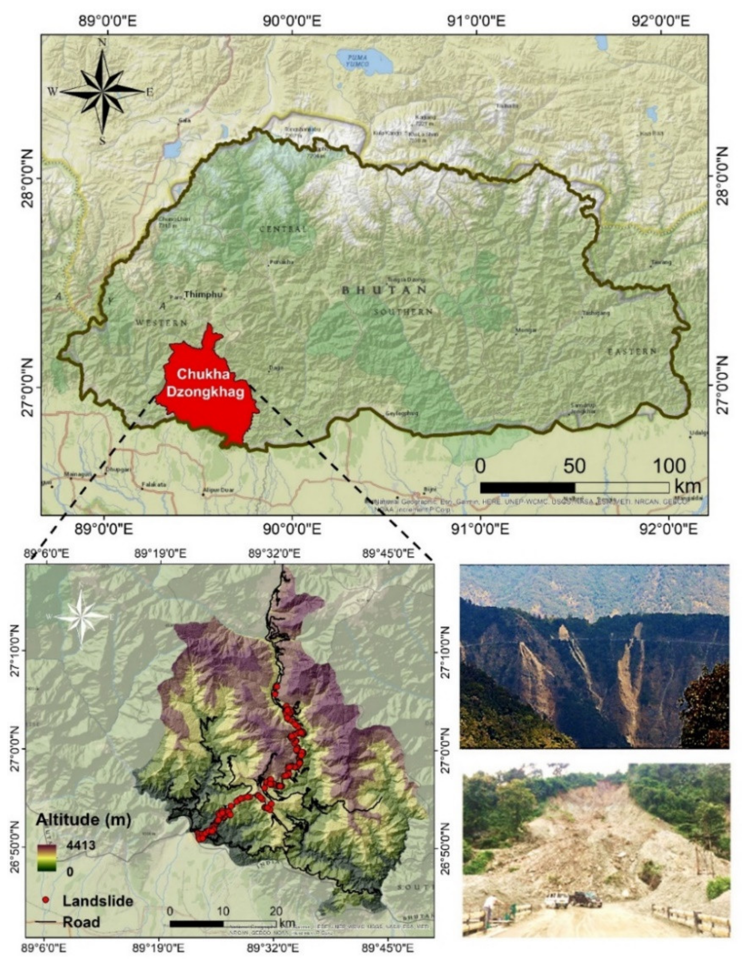
3.1. Study Area
3.2. Datasets
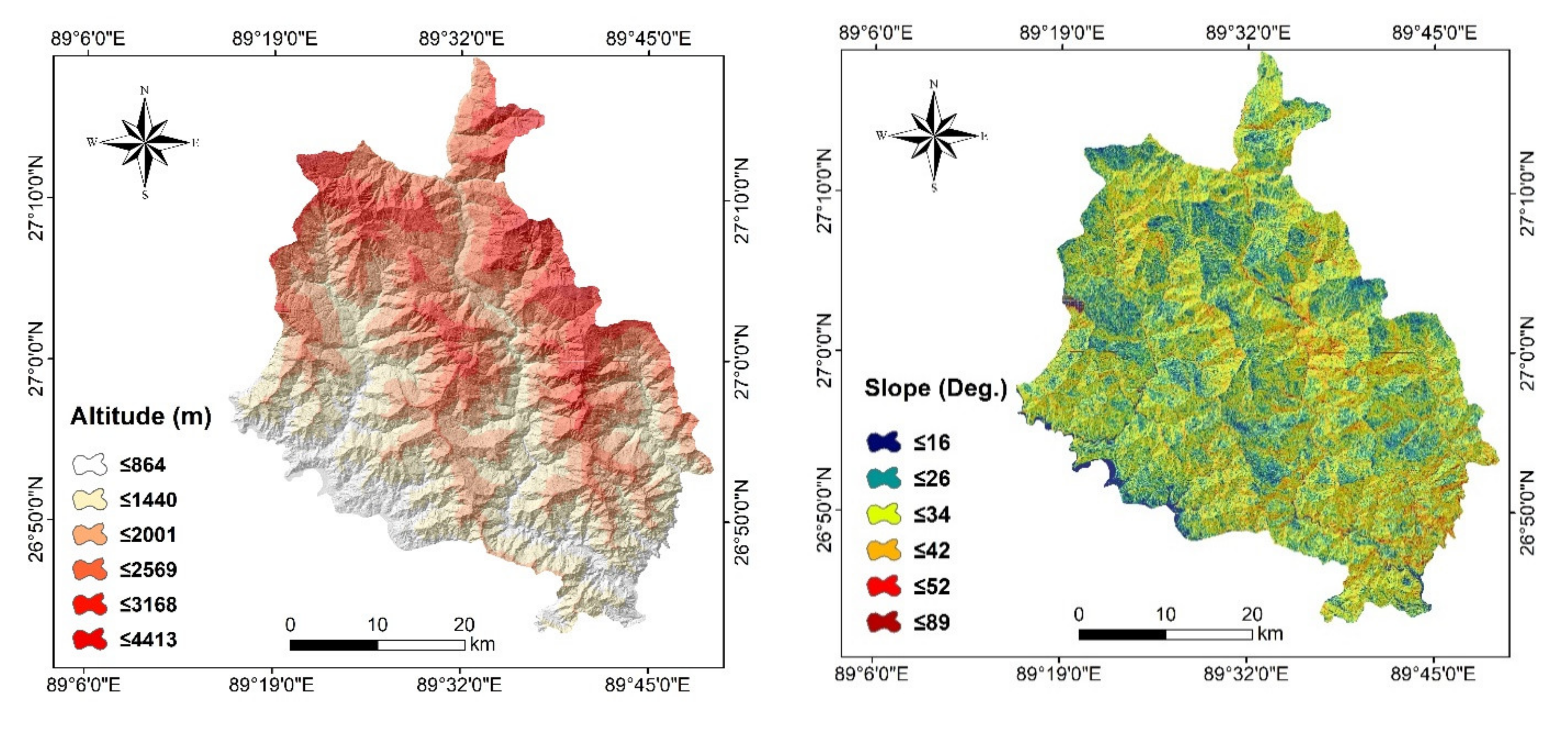
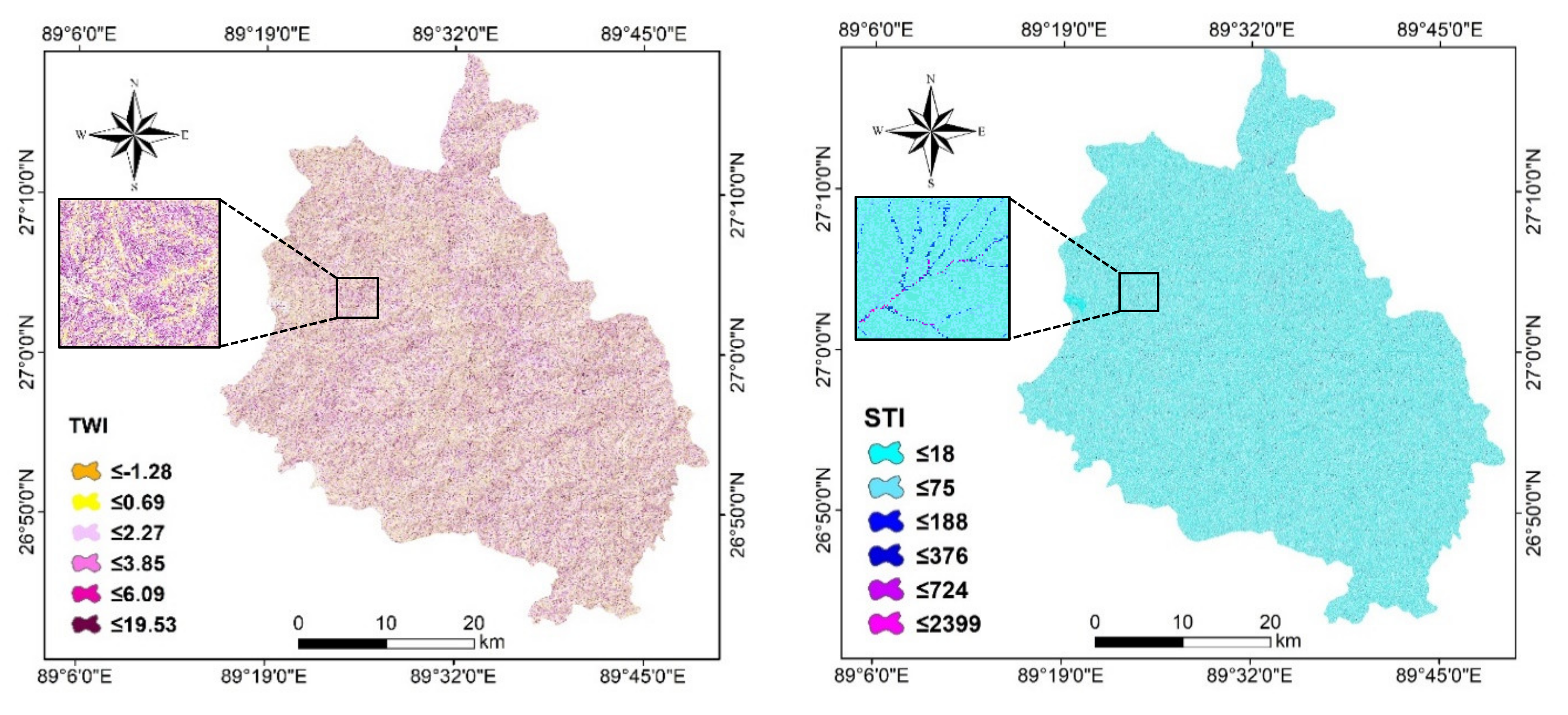
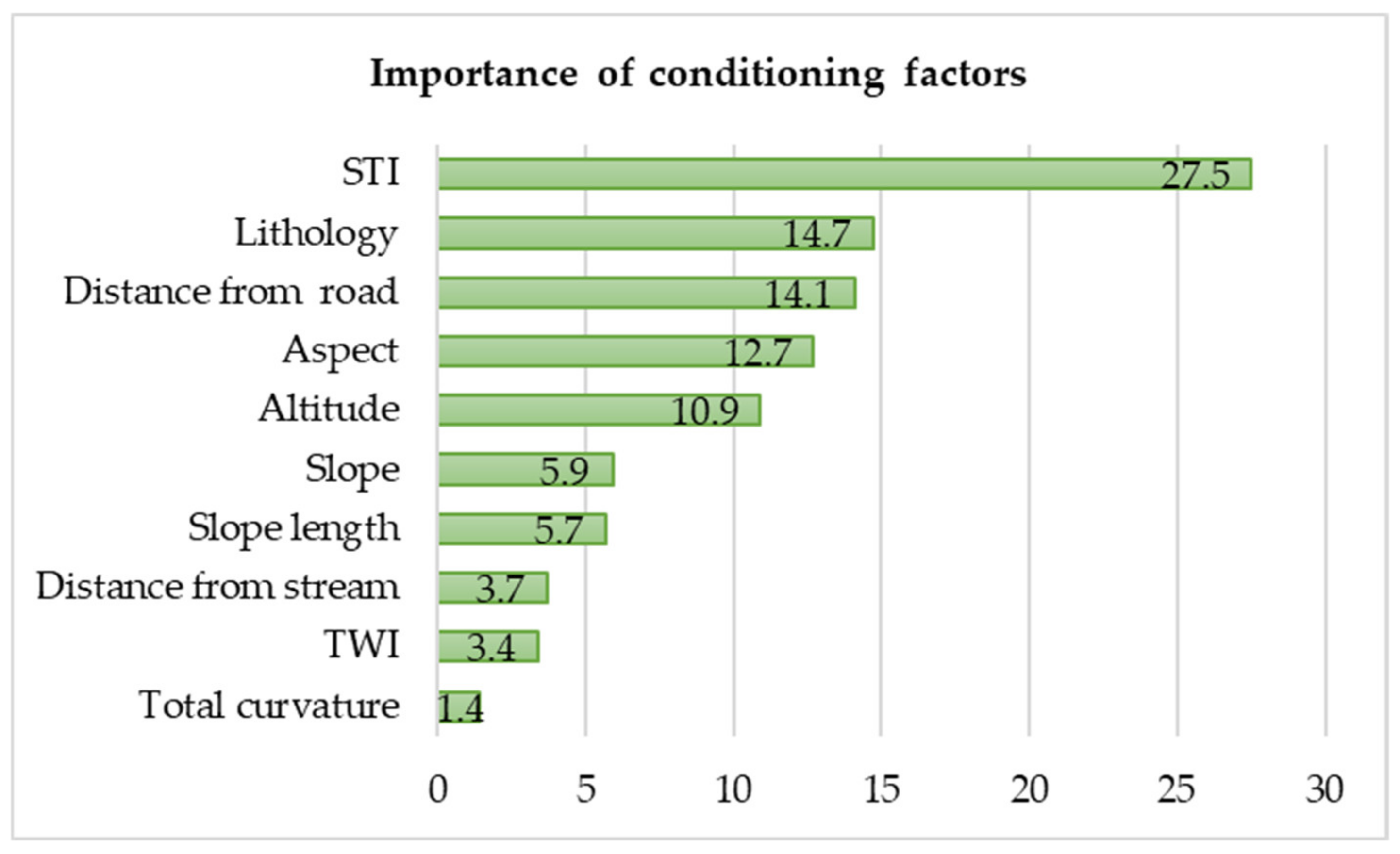
3.2.1. Geodatabase of Conditioning Factors
3.2.2. Landslide Inventory Dataset
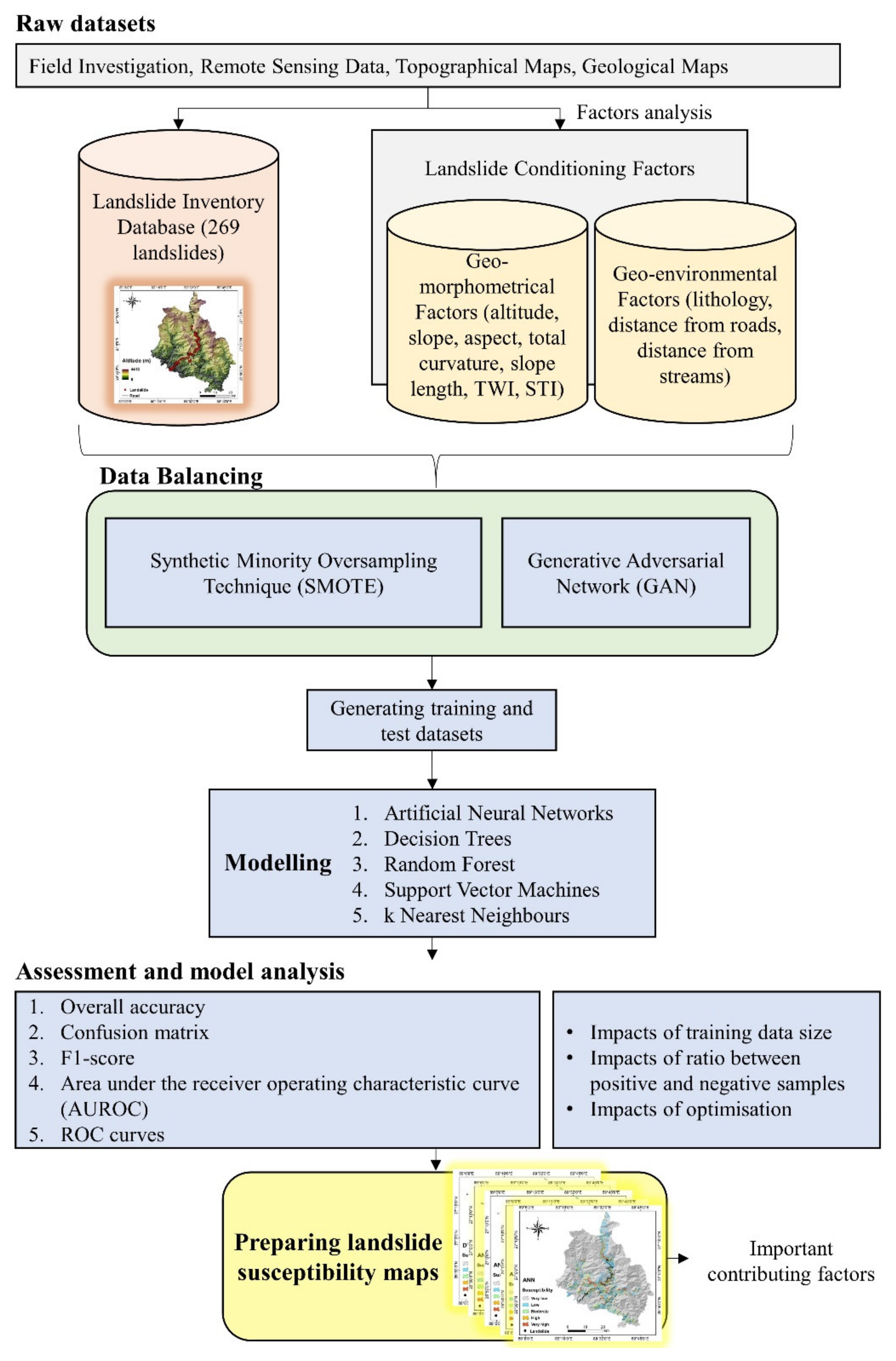
3.3. Methodology
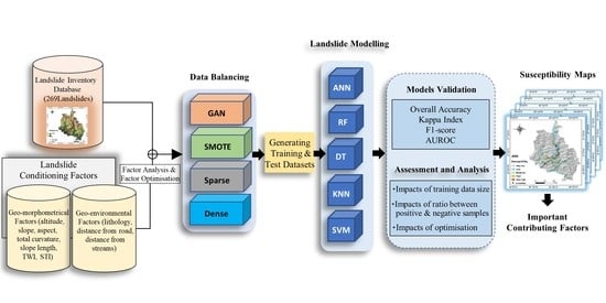
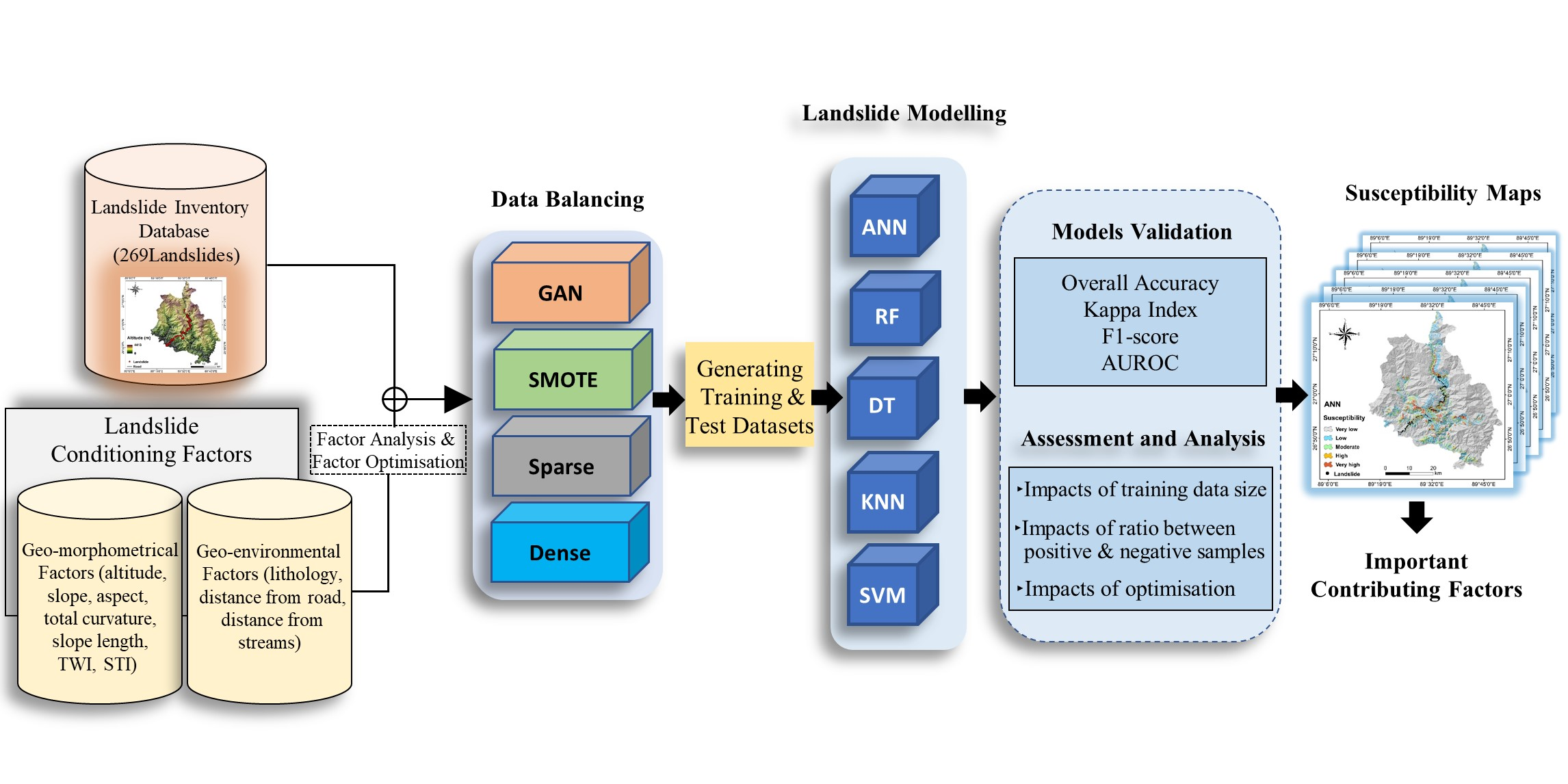
3.3.1. Overview
3.3.2. Data Balancing
- a.
- Synthetic Minority Oversampling Technique (SMOTE)
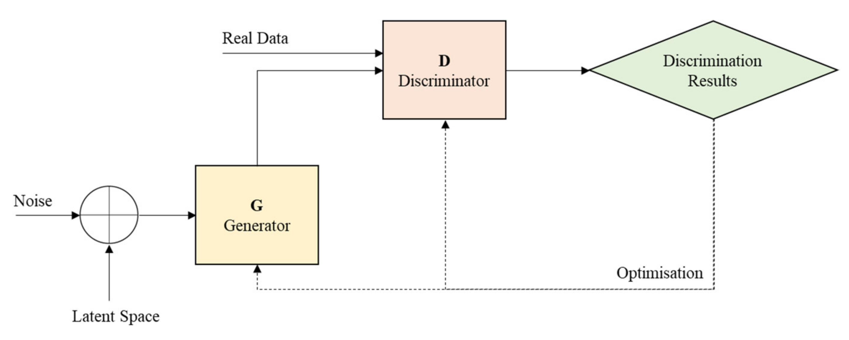
- b.
- Generative Adversarial Network (GAN)
3.3.3. Machine Learning Models
Artificial Neural Networks (ANN)
Decision Trees (DT)
Random Forests (RF)
Support Vector Machines (SVM)
k Nearest Neighbours (kNN)
3.3.4. Assessment and Model Analysis
- a.
- Accuracy metrics
- i.
- Overall accuracy (OA)
- ii.
- Confusion matrix
- iii.
- F1-score
- iv.
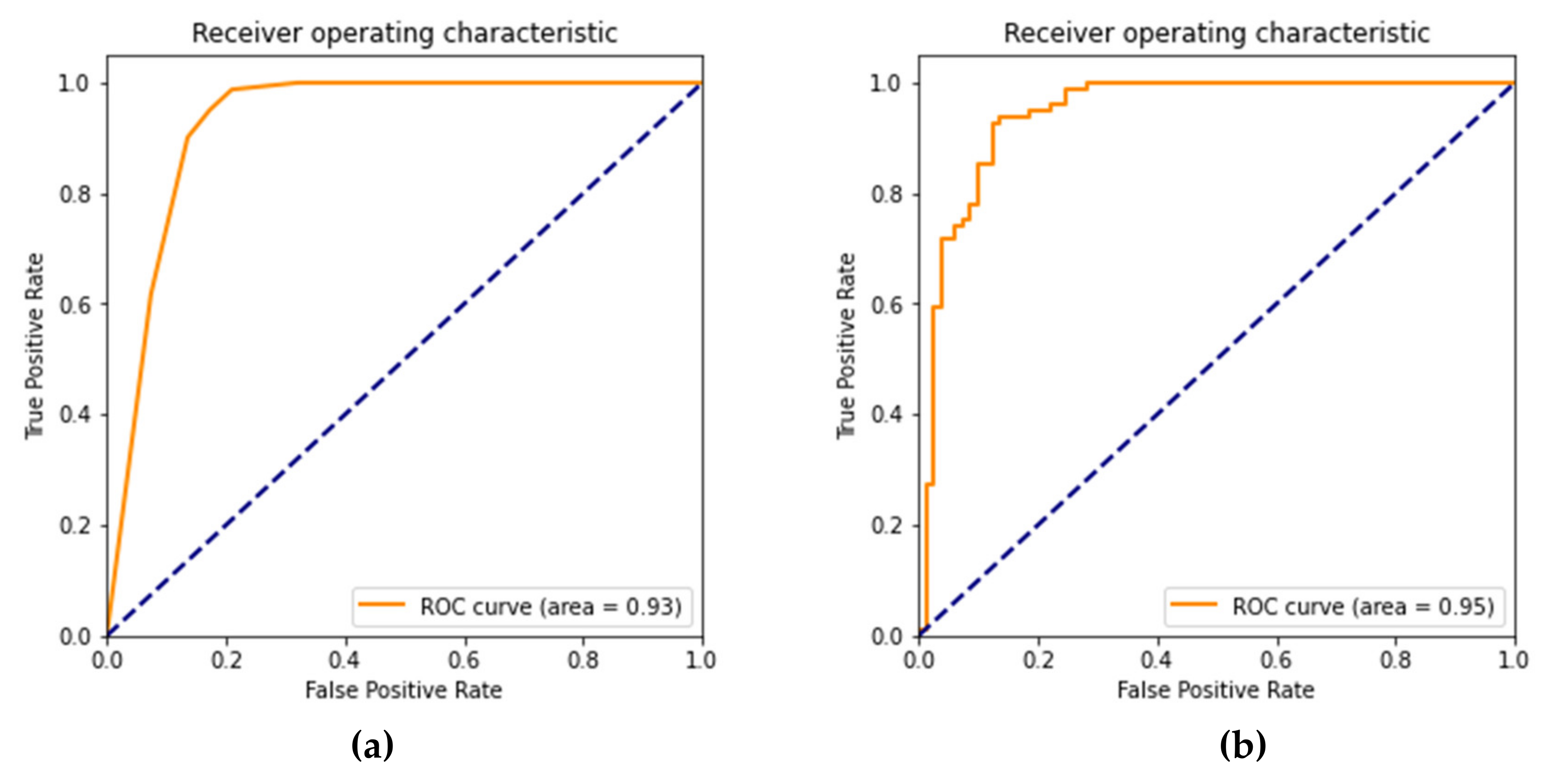
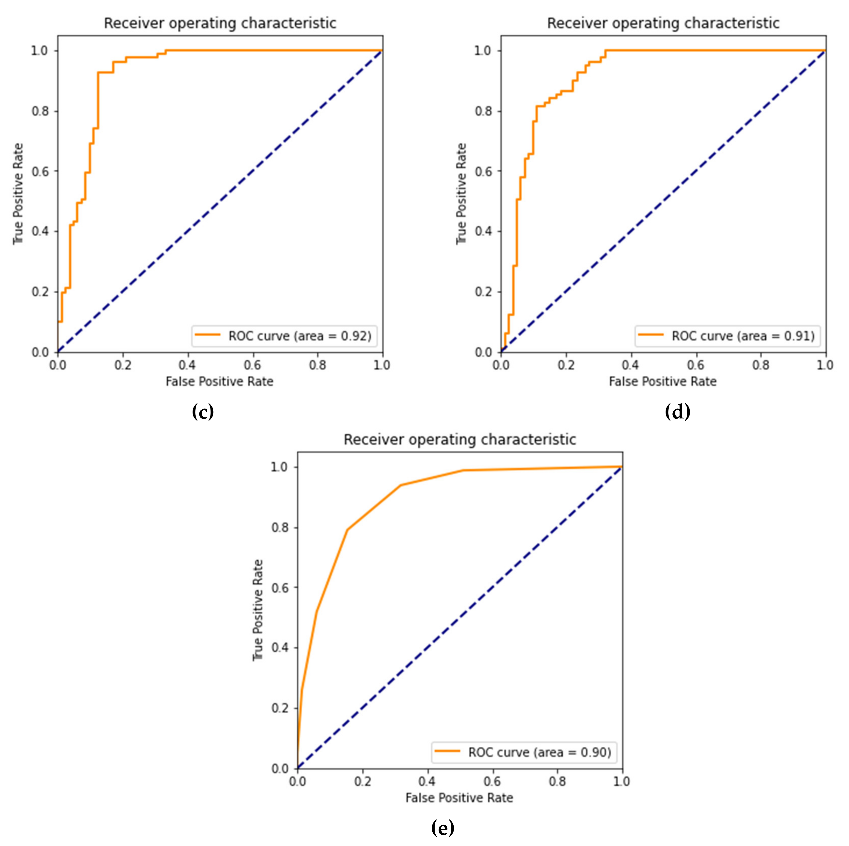
- Area under the receiver operating characteristic curve (AUROC)
- b.
- Model analysis
- Impacts of training data size: The quantity of training samples affects the machine learning models’ performance [57]. Thus, we conducted an experiment to understand how each model is impacted by the size of the training dataset. Also, this experiment was performed to understand how data balancing methods work with different sizes of training samples.
- Impacts of the ratio between positive and negative samples: The ratio between the positive and negative samples has a great impact on the machine learning models’ performance. As a result, this experiment was performed to understand how each model is impacted by the ratio between the landslide and non-landslide samples.
- Impacts of model’s optimisation: Several hyperparameters for each machine learning model were employed in this research. Those require optimisation to achieve the best performance for the model and also to improve their generalisation in unknown areas. Thus, this experiment was conducted to study the impact of model optimisation on the accuracy of the landslide susceptibility maps.
3.3.5. Preparing Landslide Susceptibility Maps
4. Results
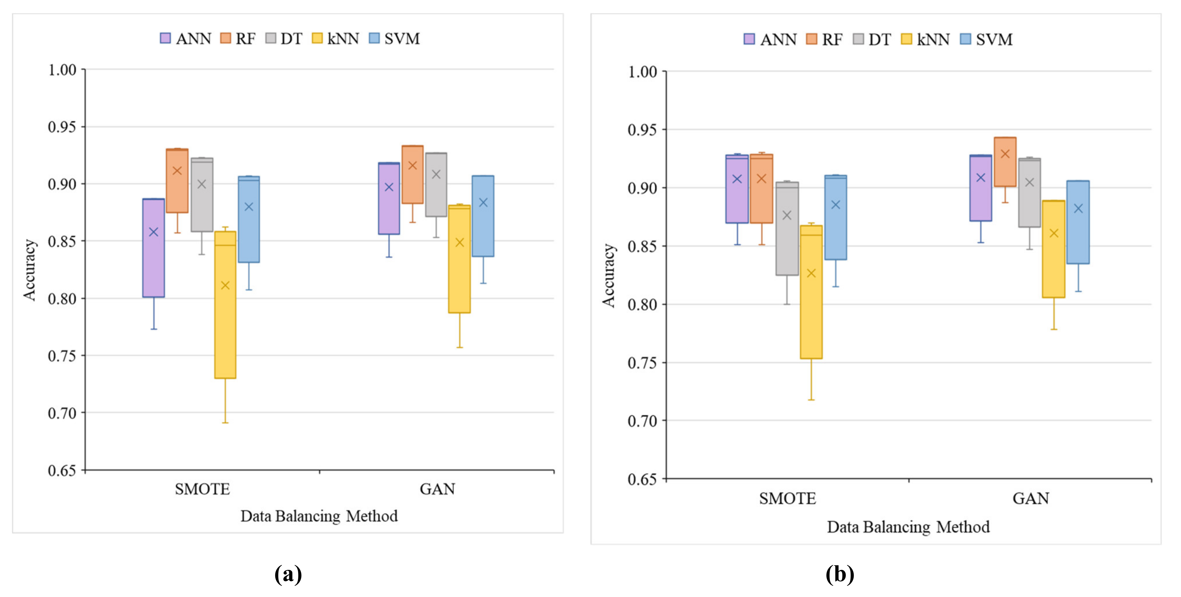
4.1. Assessing Data Balancing Methods, i.e., SMOTE and GAN
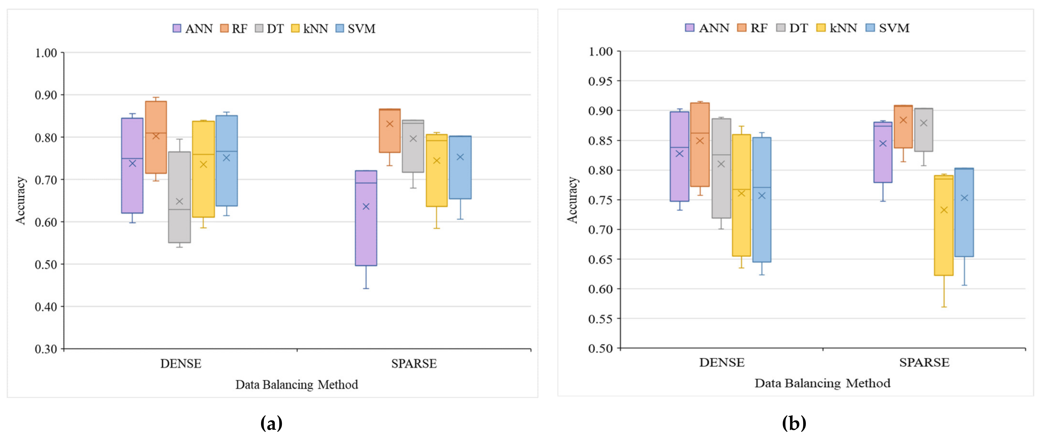
4.2. Assessment and Comparison of used Models
4.3. Model Analysis
4.3.1. Analysis of Optimisation Impact on Machine Learning Models
4.3.2. Analysis of Training Data Size Impact on Machine Learning Models
4.3.3. Analysis of Landslide to Non-Landslide Sample Ratio Impact on Machine Learning Models
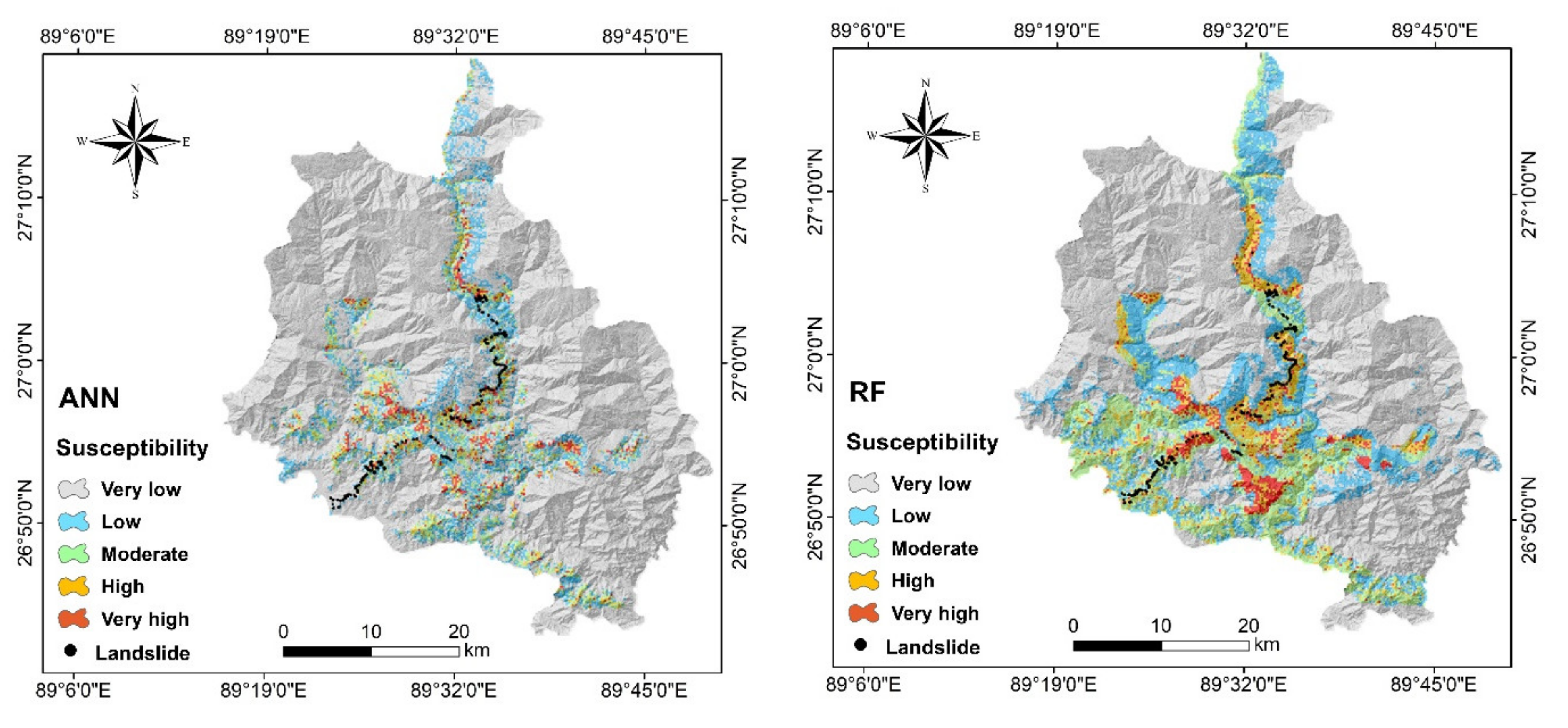
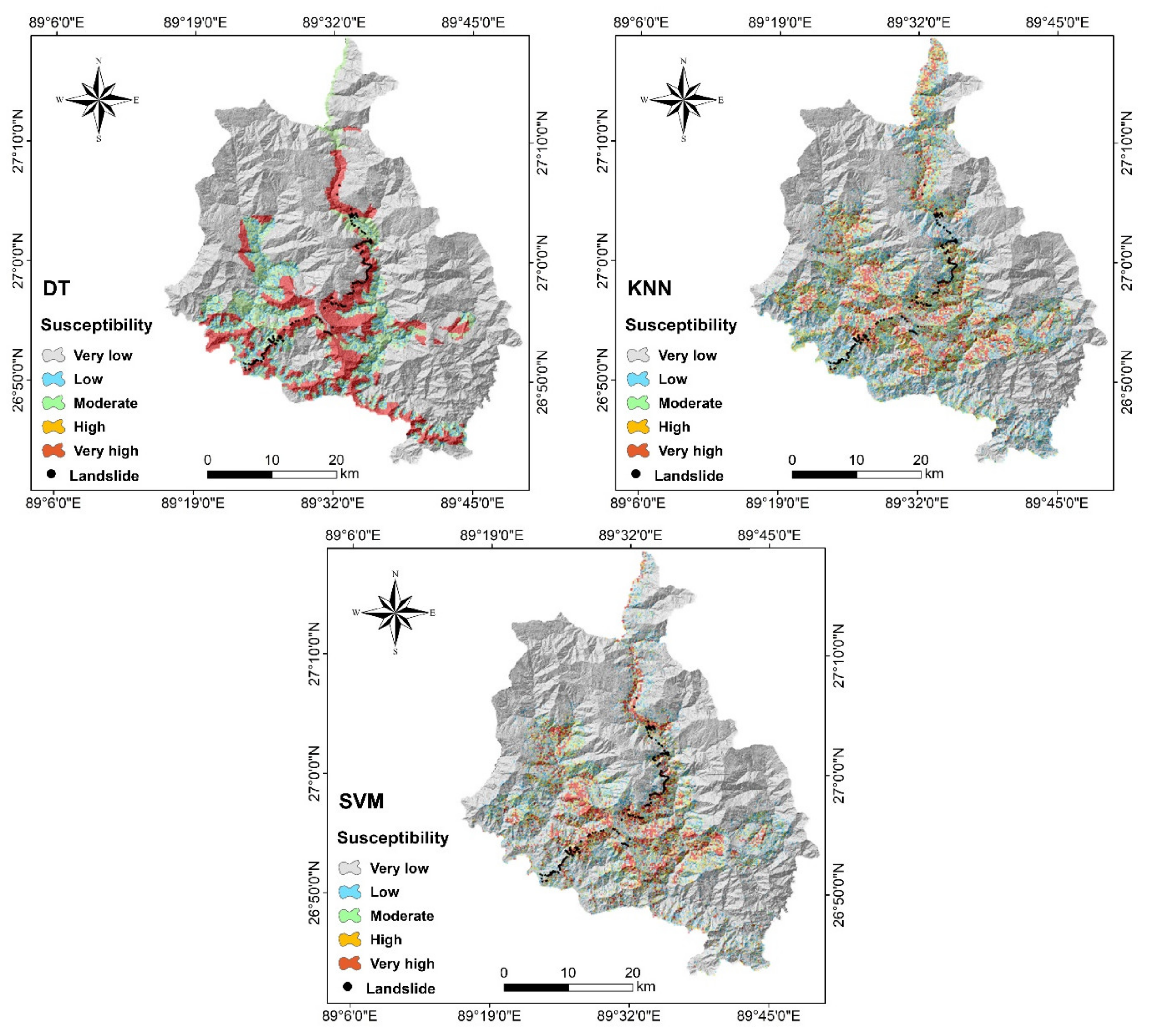
4.4. Spatial Prediction of Landslides with Machine Learning Models
5. Discussion
6. Conclusions
Author Contributions
Funding
Data Availability Statement
Acknowledgments
Conflicts of Interest
List of Abbreviations
| DI | data imbalance |
| GAN | generative adversarial networks |
| SMOTE | synthetic minority oversampling technique |
| ANN | artificial neural networks |
| RF | random forests |
| DT | decision trees |
| kNN | k-nearest neighbours |
| SVM | support vector machine |
| OA | overall accuracy |
| AUROC | area under receiver operating characteristic curves |
| TWI | topographic wetness index |
| STI | sediment transport index |
| FDA | fisher discriminant analysis |
| ADASYN | adaptive synthetic sampling approach for imbalanced learning |
| LDA | linear discriminant analysis |
| DEM | digital elevation model |
| ALOS | advanced land observing satellite |
| PALSAR | the phased array L-band synthetic aperture radar |
Appendix A

| Parameters | Model | Sampling Method | |||
|---|---|---|---|---|---|
| Dense Samples | Sparse Samples | SMOTE | GAN | ||
| Default | ANN | 0.856 | 0.721 | 0.887 | 0.918 |
| RF | 0.894 | 0.866 | 0.929 | 0.933 | |
| DT | 0.854 | 0.840 | 0.919 | 0.927 | |
| kNN | 0.840 | 0.792 | 0.846 | 0.878 | |
| SVM | 0.859 | 0.803 | 0.903 | 0.907 | |
| Optimal | ANN | 0.903 | 0.874 | 0.925 | 0.927 |
| RF | 0.908 | 0.907 | 0.925 | 0.943 | |
| DT | 0.889 | 0.903 | 0.900 | 0.923 | |
| kNN | 0.874 | 0.784 | 0.859 | 0.889 | |
| SVM | 0.863 | 0.803 | 0.908 | 0.906 | |
| Parameters | Model | Sampling Method | |||
|---|---|---|---|---|---|
| Dense Samples | Sparse Samples | SMOTE | GAN | ||
| Default | ANN | 0.597 | 0.442 | 0.773 | 0.836 |
| RF | 0.697 | 0.732 | 0.857 | 0.866 | |
| DT | 0.582 | 0.68 | 0.838 | 0.853 | |
| kNN | 0.585 | 0.584 | 0.691 | 0.757 | |
| SVM | 0.614 | 0.606 | 0.807 | 0.813 | |
| Optimal | ANN | 0.732 | 0.747 | 0.851 | 0.853 |
| RF | 0.757 | 0.814 | 0.851 | 0.887 | |
| DT | 0.701 | 0.807 | 0.800 | 0.847 | |
| kNN | 0.635 | 0.569 | 0.718 | 0.778 | |
| SVM | 0.623 | 0.606 | 0.815 | 0.811 | |
| Parameters | Model | Sampling Method | |||
|---|---|---|---|---|---|
| Dense Samples | Sparse Samples | SMOTE | GAN | ||
| Default | ANN | 0.690 | 0.661 | 0.885 | 0.916 |
| RF | 0.765 | 0.862 | 0.931 | 0.932 | |
| DT | 0.676 | 0.826 | 0.923 | 0.926 | |
| kNN | 0.690 | 0.811 | 0.862 | 0.882 | |
| SVM | 0.705 | 0.800 | 0.907 | 0.907 | |
| Optimal | ANN | 0.794 | 0.883 | 0.929 | 0.928 |
| RF | 0.817 | 0.909 | 0.930 | 0.943 | |
| DT | 0.773 | 0.904 | 0.906 | 0.926 | |
| kNN | 0.716 | 0.793 | 0.870 | 0.888 | |
| SVM | 0.712 | 0.800 | 0.911 | 0.906 | |
| Parameters | Model | Sampling Method | |||
|---|---|---|---|---|---|
| Dense Samples | Sparse Samples | SMOTE | GAN | ||
| Default | ANN | 0.809 | 0.721 | 0.887 | 0.918 |
| RF | 0.855 | 0.866 | 0.929 | 0.933 | |
| DT | 0.795 | 0.840 | 0.919 | 0.927 | |
| kNN | 0.828 | 0.792 | 0.846 | 0.878 | |
| SVM | 0.825 | 0.803 | 0.903 | 0.907 | |
| Optimal | ANN | 0.882 | 0.874 | 0.925 | 0.93 |
| RF | 0.915 | 0.907 | 0.925 | 0.95 | |
| DT | 0.878 | 0.903 | 0.900 | 0.923 | |
| kNN | 0.818 | 0.785 | 0.859 | 0.91 | |
| SVM | 0.830 | 0.803 | 0.908 | 0.906 | |
Appendix B
| Sampling | Model | Training Size | |||
|---|---|---|---|---|---|
| 0.3 | 0.5 | 0.7 | 0.9 | ||
| Dense | ANN | 0.855 | 0.903 | 0.918 | 0.894 |
| RF | 0.892 | 0.908 | 0.924 | 0.902 | |
| DT | 0.904 | 0.889 | 0.899 | 0.878 | |
| kNN | 0.832 | 0.874 | 0.872 | 0.837 | |
| SVM | 0.843 | 0.863 | 0.880 | 0.862 | |
| Sparse | ANN | 0.836 | 0.874 | 0.870 | 0.833 |
| RF | 0.881 | 0.907 | 0.914 | 0.907 | |
| DT | 0.889 | 0.903 | 0.907 | 0.907 | |
| kNN | 0.769 | 0.784 | 0.833 | 0.759 | |
| SVM | 0.780 | 0.803 | 0.852 | 0.796 | |
| SMOTE | ANN | 0.921 | 0.925 | 0.935 | 0.932 |
| RF | 0.920 | 0.925 | 0.941 | 0.948 | |
| DT | 0.900 | 0.900 | 0.899 | 0.916 | |
| kNN | 0.839 | 0.859 | 0.874 | 0.885 | |
| SVM | 0.903 | 0.908 | 0.913 | 0.911 | |
| GAN | ANN | 0.898 | 0.927 | 0.937 | 0.916 |
| RF | 0.939 | 0.943 | 0.946 | 0.942 | |
| DT | 0.929 | 0.924 | 0.934 | 0.942 | |
| kNN | 0.890 | 0.889 | 0.897 | 0.890 | |
| SVM | 0.900 | 0.906 | 0.900 | 0.880 | |
| Sampling | Model | Training Size | |||
|---|---|---|---|---|---|
| 0.3 | 0.5 | 0.7 | 0.9 | ||
| Dense | ANN | 0.579 | 0.732 | 0.766 | 0.703 |
| RF | 0.711 | 0.757 | 0.795 | 0.723 | |
| DT | 0.737 | 0.701 | 0.723 | 0.658 | |
| kNN | 0.494 | 0.635 | 0.612 | 0.512 | |
| SVM | 0.568 | 0.623 | 0.666 | 0.612 | |
| Sparse | ANN | 0.671 | 0.747 | 0.741 | 0.667 |
| RF | 0.761 | 0.814 | 0.827 | 0.815 | |
| DT | 0.783 | 0.807 | 0.815 | 0.815 | |
| kNN | 0.539 | 0.569 | 0.667 | 0.519 | |
| SVM | 0.560 | 0.606 | 0.704 | 0.593 | |
| SMOTE | ANN | 0.842 | 0.851 | 0.871 | 0.864 |
| RF | 0.839 | 0.851 | 0.881 | 0.895 | |
| DT | 0.800 | 0.800 | 0.797 | 0.833 | |
| kNN | 0.677 | 0.718 | 0.748 | 0.770 | |
| SVM | 0.806 | 0.815 | 0.825 | 0.822 | |
| GAN | ANN | 0.796 | 0.853 | 0.874 | 0.832 |
| RF | 0.879 | 0.887 | 0.892 | 0.885 | |
| DT | 0.858 | 0.847 | 0.867 | 0.885 | |
| kNN | 0.780 | 0.778 | 0.794 | 0.780 | |
| SVM | 0.799 | 0.811 | 0.801 | 0.759 | |
| Sampling | Model | Training Size | |||
|---|---|---|---|---|---|
| 0.3 | 0.5 | 0.7 | 0.9 | ||
| Dense | ANN | 0.672 | 0.794 | 0.819 | 0.772 |
| RF | 0.781 | 0.817 | 0.844 | 0.786 | |
| DT | 0.799 | 0.773 | 0.789 | 0.737 | |
| kNN | 0.600 | 0.716 | 0.693 | 0.615 | |
| SVM | 0.670 | 0.712 | 0.744 | 0.702 | |
| Sparse | ANN | 0.846 | 0.883 | 0.879 | 0.830 |
| RF | 0.887 | 0.909 | 0.916 | 0.912 | |
| DT | 0.897 | 0.904 | 0.911 | 0.909 | |
| kNN | 0.776 | 0.793 | 0.838 | 0.755 | |
| SVM | 0.774 | 0.800 | 0.852 | 0.784 | |
| SMOTE | ANN | 0.926 | 0.929 | 0.938 | 0.935 |
| RF | 0.924 | 0.930 | 0.943 | 0.950 | |
| DT | 0.908 | 0.906 | 0.905 | 0.922 | |
| kNN | 0.855 | 0.870 | 0.884 | 0.894 | |
| SVM | 0.907 | 0.911 | 0.916 | 0.913 | |
| GAN | ANN | 0.900 | 0.928 | 0.937 | 0.917 |
| RF | 0.940 | 0.943 | 0.946 | 0.942 | |
| DT | 0.931 | 0.927 | 0.936 | 0.943 | |
| kNN | 0.889 | 0.888 | 0.896 | 0.888 | |
| SVM | 0.903 | 0.906 | 0.901 | 0.883 | |
| Sampling | Model | Training Size | |||
|---|---|---|---|---|---|
| 0.3 | 0.5 | 0.7 | 0.9 | ||
| Dense | ANN | 0.791 | 0.882 | 0.890 | 0.866 |
| RF | 0.885 | 0.915 | 0.929 | 0.871 | |
| DT | 0.891 | 0.878 | 0.882 | 0.842 | |
| kNN | 0.739 | 0.818 | 0.794 | 0.749 | |
| SVM | 0.800 | 0.830 | 0.848 | 0.818 | |
| Sparse | ANN | 0.836 | 0.874 | 0.870 | 0.833 |
| RF | 0.881 | 0.907 | 0.914 | 0.907 | |
| DT | 0.889 | 0.903 | 0.907 | 0.907 | |
| kNN | 0.769 | 0.785 | 0.833 | 0.759 | |
| SVM | 0.780 | 0.803 | 0.852 | 0.796 | |
| SMOTE | ANN | 0.921 | 0.925 | 0.935 | 0.932 |
| RF | 0.920 | 0.925 | 0.941 | 0.948 | |
| DT | 0.900 | 0.900 | 0.899 | 0.917 | |
| kNN | 0.839 | 0.859 | 0.874 | 0.885 | |
| SVM | 0.903 | 0.908 | 0.913 | 0.911 | |
| GAN | ANN | 0.898 | 0.927 | 0.937 | 0.916 |
| RF | 0.939 | 0.943 | 0.946 | 0.942 | |
| DT | 0.929 | 0.923 | 0.934 | 0.942 | |
| kNN | 0.890 | 0.889 | 0.897 | 0.890 | |
| SVM | 0.900 | 0.906 | 0.900 | 0.880 | |
References
- Turner, A.K. Social and environmental impacts of landslides. Innov. Infrastruct. Solut. 2018, 3, 1–25. [Google Scholar] [CrossRef]
- Sidle, R.C. Using Weather and Climate Information for Landslide Prevention and Mitigation. Climate and Land Degradation; Springer: Berlin/Heidelberg, Germany, 2007; pp. 285–307. [Google Scholar] [CrossRef]
- Mezaal, M.R.; Pradhan, B.; Sameen, M.I.; Shafri, H.Z.M.; Yusoff, Z.M. Optimized Neural Architecture for Automatic Landslide Detection from High-Resolution Airborne Laser Scanning Data. Appl. Sci. 2017, 7, 730. [Google Scholar] [CrossRef] [Green Version]
- Froude, M.J.; Petley, D.N. Global fatal landslide occurrence from 2004 to 2016. Nat. Hazards Earth Syst. Sci. 2018, 18, 2161–2181. [Google Scholar] [CrossRef] [Green Version]
- Dikshit, A.; Sarkar, R.; Pradhan, B.; Jena, R.; Drukpa, D.; Alamri, A.M. Temporal Probability Assessment and Its Use in Landslide Susceptibility Mapping for Eastern Bhutan. Water 2020, 12, 267. [Google Scholar] [CrossRef] [Green Version]
- United Nations Department of Economic and Social Affairs. World Economic Situation and Prospects 2019. 2019. Available online: https://www.un.org/development/desa/dpad/wp-content/uploads/sites/45/WESP2019_BOOK-web.pdf (accessed on 1 September 2021).
- Lee, J.-H.; Sameen, M.I.; Pradhan, B.; Park, H.-J. Modeling landslide susceptibility in data-scarce environments using optimized data mining and statistical methods. Geomorphology 2018, 303, 284–298. [Google Scholar] [CrossRef]
- Yang, Y.; Yang, J.; Xu, C.; Xu, C.; Song, C. Local-scale landslide susceptibility mapping using the B-GeoSVC model. Landslides 2019, 16, 1301–1312. [Google Scholar] [CrossRef]
- Zhao, X.; Chen, W. Optimization of Computational Intelligence Models for Landslide Susceptibility Evaluation. Remote Sens. 2020, 12, 2180. [Google Scholar] [CrossRef]
- Kavzoglu, T.; Sahin, E.K.; Colkesen, I. Selecting optimal conditioning factors in shallow translational landslide susceptibility mapping using genetic algorithm. Eng. Geol. 2015, 192, 101–112. [Google Scholar] [CrossRef]
- Zhang, S.; Ren, W.; Zhang, X.; Liu, H. Prediction Method of Landslide Disaster in Southern China Based on Multi Attribute Group Decision Making, Proceedings of the 2016 6th International Conference on Machinery, Materials, Environment, Biotechnology and Computer; Atlantis Press: Amsterdam, The Netherlands, 2016; pp. 2078–2083. [Google Scholar]
- Hussin, H.Y.; Zumpano, V.; Reichenbach, P.; Sterlacchini, S.; Micu, M.; van Westen, C.; Bălteanu, D. Different landslide sampling strategies in a grid-based bi-variate statistical susceptibility model. Geomorphology 2016, 253, 508–523. [Google Scholar] [CrossRef]
- Lai, J.-S.; Chiang, S.-H.; Tsai, F. Exploring Influence of Sampling Strategies on Event-Based Landslide Susceptibility Modeling. ISPRS Int. J. Geo-Inf. 2019, 8, 397. [Google Scholar] [CrossRef] [Green Version]
- Zhu, A.-X.; Miao, Y.; Liu, J.; Bai, S.; Zeng, C.; Ma, T.; Hong, H. A similarity-based approach to sampling absence data for landslide susceptibility mapping using data-driven methods. Catena 2019, 183, 104188. [Google Scholar] [CrossRef]
- Pourghasemi, H.R.; Kornejady, A.; Kerle, N.; Shabani, F. Investigating the effects of different landslide positioning techniques, landslide partitioning approaches, and presence-absence balances on landslide susceptibility mapping. Catena 2020, 187, 104364. [Google Scholar] [CrossRef]
- Chowdhuri, I.; Pal, S.C.; Arabameri, A.; Ngo, P.T.T.; Chakrabortty, R.; Malik, S.; Das, B.; Roy, P. Ensemble approach to develop landslide susceptibility map in landslide dominated Sikkim Himalayan region, India. Environ. Earth Sci. 2020, 79, 1–28. [Google Scholar] [CrossRef]
- Di Napoli, M.; Carotenuto, F.; Cevasco, A.; Confuorto, P.; Di Martire, D.; Firpo, M.; Pepe, G.; Raso, E.; Calcaterra, D. Machine learning ensemble modelling as a tool to improve landslide susceptibility mapping reliability. Landslides 2020, 17, 1897–1914. [Google Scholar] [CrossRef]
- Al-Najjar, H.A.; Pradhan, B. Spatial landslide susceptibility assessment using machine learning techniques assisted by additional data created with generative adversarial networks. Geosci. Front. 2021, 12, 625–637. [Google Scholar] [CrossRef]
- Taalab, K.; Cheng, T.; Zhang, Y. Mapping landslide susceptibility and types using Random Forest. Big Earth Data 2018, 2, 159–178. [Google Scholar] [CrossRef]
- Gupta, S.K.; Jhunjhunwalla, M.; Bhardwaj, A.; Shukla, D.P. Data imbalance in landslide susceptibility zonation: Under-sampling for class-imbalance learning. Int. Arch. Photogramm. Remote Sens. Spat. Inf. Sci. 2020, XLII-3/W11, 51–57. [Google Scholar] [CrossRef] [Green Version]
- Guzzetti, F.; Reichenbach, P.; Cardinali, M.; Galli, M.; Ardizzone, F. Probabilistic landslide hazard assessment at the basin scale. Geomorphol. 2005, 72, 272–299. [Google Scholar] [CrossRef]
- Krawczyk, B. Learning from imbalanced data: Open challenges and future directions. Prog. Artif. Intell. 2016, 5, 221–232. [Google Scholar] [CrossRef] [Green Version]
- He, H.; Garcia, E.A. Learning from Imbalanced Data. IEEE Trans. Knowl. Data Eng. 2009, 21, 1263–1284. [Google Scholar] [CrossRef]
- Chawla, N.V. Data Mining for Imbalanced Datasets: An Overview. Data Min. Knowl. Discov. Handb. 2009, 2009, 875–886. [Google Scholar] [CrossRef] [Green Version]
- Galar, M.; Fernandez, A.; Barrenechea, E.; Bustince, H.; Herrera, F. A Review on Ensembles for the Class Imbalance Problem: Bagging-, Boosting-, and Hybrid-Based Approaches. IEEE Trans. Syst. Man Cybern. Part C (Appl. Rev.) 2012, 42, 463–484. [Google Scholar] [CrossRef]
- Haixiang, G.; Yijing, L.; Shang, J.; Mingyun, G.; Yuanyue, H.; Bing, G. Learning from class-imbalanced data: Review of methods and applications. Expert Syst. Appl. 2017, 73, 220–239. [Google Scholar] [CrossRef]
- Stumpf, A.; Lachiche, N.; Kerle, N.; Malet, J.-P.; Puissant, A. Adaptive spatial sampling with active random forest for object-oriented landslide mapping. In Proceedings of the 2012 IEEE International Geoscience and Remote Sensing Symposium, Munich, Germany, 22–27 July 2012; pp. 87–90. [Google Scholar] [CrossRef]
- Stumpf, A.; Lachiche, N.; Malet, J.-P.; Kerle, N.; Puissant, A. Active Learning in the Spatial Domain for Remote Sensing Image Classification. IEEE Trans. Geosci. Remote Sens. 2013, 52, 2492–2507. [Google Scholar] [CrossRef]
- Goodfellow, I.; Pouget-Abadie, J.; Mirza, M.; Xu, B.; Warde-Farley, D.; Ozair, S.; Courville, A.; Bengio, Y. Generative adversarial nets. In Proceedings of the Annual Conference on Neural Information Processing Systems, Montreal, QC, Canada, 8–13 December 2014; pp. 2672–2680. [Google Scholar]
- Chawla, N.V.; Bowyer, K.W.; Hall, L.O.; Kegelmeyer, W.P. SMOTE: Synthetic Minority Over-sampling Technique. J. Artif. Intell. Res. 2002, 16, 321–357. [Google Scholar] [CrossRef]
- Tsangaratos, P.; Ilia, I. Landslide susceptibility mapping using a modified decision tree classifier in the Xanthi Perfection, Greece. Landslides 2016, 13, 305–320. [Google Scholar] [CrossRef]
- Pyle, D. Business Modeling and Data Mining; Morgan Kaufmann Publishers: Burlington, MA, USA, 2003. [Google Scholar]
- Agrawal, K.; Baweja, Y.; Dwivedi, D.; Saha, R.; Prasad, P.; Agrawal, S.; Kapoor, S.; Chaturvedi, P.; Mali, N.; Kala, V.U.; et al. A Comparison of Class Imbalance Techniques for Real-World Landslide Predictions. In Proceedings of the 2017 International Conference on Machine Learning and Data Science (MLDS), IEEE, Noida, India, 14–15 December 2017; pp. 1–8. [Google Scholar]
- Zhao, L.; Wu, X.; Niu, R.; Wang, Y.; Zhang, K. Using the rotation and random forest models of ensemble learning to predict landslide susceptibility. Geomat. Nat. Hazards Risk 2020, 11, 1542–1564. [Google Scholar] [CrossRef]
- Braun, A.; Garcia-Urquia, E.L.; Lopez, R.M.; Yamagishi, H. Landslide Susceptibility Mapping in Tegucigalpa, Honduras, Using Data Mining Methods. In Proceedings of the IAEG/AEG Annual Meeting Proceedings, San Francisco, CA, USA, 2018, Volume 1; Springer: Cham, Switzerland, 2019; pp. 207–215. [Google Scholar] [CrossRef]
- Mutlu, A.; Goz, F. SkySlide: A Hybrid Method for Landslide Susceptibility Assessment based on Landslide-Occurring Data Only. Comput. J. 2020, 2020, bxaa063. [Google Scholar] [CrossRef]
- Zhang, S.; Yu, P. Seismic landslide susceptibility assessment based on ADASYN-LDA model. In Proceedings of the IOP Conference Series: Earth and Environmental Science, 5th International Conference on Minerals Source, Geotechnology and Civil Engineering, Guiyang, China, 17–19 April 2020; IOP Publishing: Bristol, UK, 2020; 525, p. 12087. [Google Scholar] [CrossRef]
- Song, Y.; Niu, R.; Xu, S.; Ye, R.; Peng, L.; Guo, T.; Li, S.; Chen, T. Landslide Susceptibility Mapping Based on Weighted Gradient Boosting Decision Tree in Wanzhou Section of the Three Gorges Reservoir Area (China). ISPRS Int. J. Geo-Inf. 2019, 8, 4. [Google Scholar] [CrossRef] [Green Version]
- Kuenza, K.; Dorji, Y.; Wangda, D. Landslides in Bhutan. In Proceedings of the SAARC Workshop on Landslide Risk Management in South Asia, Thimphu, Bhutan, 11–12 May 2010; UN Office for Disaster Risk Reduction (UNDRR): Geneva, Switzerland, 2010; pp. 73–80. Available online: https://www.preventionweb.net/files/14793_SAARClandslide.pdf (accessed on 1 August 2021).
- Cardarilli, M.; Lombardi, M.; Corazza, A. Landslide risk management through spatial analysis and stochastic prediction for territorial resilience evaluation. Int. J. Saf. Secur. Eng. 2019, 9, 109–120. [Google Scholar] [CrossRef] [Green Version]
- Gariano, S.L.; Sarkar, R.; Dikshit, A.; Dorji, K.; Brunetti, M.T.; Peruccacci, S.; Melillo, M. Automatic calculation of rainfall thresholds for landslide occurrence in Chukha Dzongkhag, Bhutan. Bull. Int. Assoc. Eng. Geol. Environ. 2018, 78, 4325–4332. [Google Scholar] [CrossRef]
- Gansser, A. Geology of the Bhutan Himalaya. In Denkschriften der Schweizerischen Naturforschenden Geselschaft; Birkhäuser Verlag: Basel, Switzerland, 1983; p. 181. [Google Scholar]
- Dikshit, A.; Sarkar, R.; Pradhan, B.; Acharya, S.; Dorji, K. Estimating Rainfall Thresholds for Landslide Occurrence in the Bhutan Himalayas. Water 2019, 11, 1616. [Google Scholar] [CrossRef] [Green Version]
- Sarkar, R.; Dorji, K. Determination of the Probabilities of Landslide Events—A Case Study of Bhutan. Hydrology 2019, 6, 52. [Google Scholar] [CrossRef] [Green Version]
- Gallant, J.C.; Wilson, J.P. Primary topographic attributes. In Terrain Analysis: Principles and Applications; Wilson, J.P., Gallant, J.C., Eds.; Wiley: New York, NY, USA, 2000; pp. 51–85. [Google Scholar]
- Greenwood, L.V.; Argles, T.W.; Parrish, R.R.; Harris, N.B.W.; Warren, C. The geology and tectonics of central Bhutan. J. Geol. Soc. 2016, 173, 352–369. [Google Scholar] [CrossRef] [Green Version]
- Giudici, P. Data Mining Model Comparison. In Data Mining and Knowledge Discovery Handbook; Springer: Boston, MA, USA. [CrossRef]
- Guzzetti, F.; Carrara, A.; Cardinali, M.; Reichenbach, P. Landslide hazard evaluation: A review of current techniques and their application in a multi-scale study, Central Italy. Geomorphology 1999, 31, 181–216. [Google Scholar] [CrossRef]
- Saito, H.; Nakayama, D.; Matsuyama, H. Comparison of landslide susceptibility based on a decision-tree model and actual landslide occurrence: The Akaishi Mountains, Japan. Geomorphology 2009, 109, 108–121. [Google Scholar] [CrossRef]
- Yeon, Y.-K.; Han, J.-G.; Ryu, K.H. Landslide susceptibility mapping in Injae, Korea, using a decision tree. Eng. Geol. 2010, 116, 274–283. [Google Scholar] [CrossRef]
- Breiman, L. Random Forests. Mach. Learn. 2001, 45, 5–32. [Google Scholar] [CrossRef] [Green Version]
- Schratz, P.; Muenchow, J.; Iturritxa, E.; Richter, J.; Brenning, A. Performance evaluation and hyperparameter tuning of statistical and machine-learning models using spatial data. arXiv 2018, arXiv:1803.11266. [Google Scholar]
- Vapnik, V.N. Constructing learning algorithms. In The Nature of Statistical Learning Theory; Springer: New York, NY, USA, 1995; pp. 119–166. [Google Scholar] [CrossRef]
- Marjanovic, M.; Kovačević, M.; Bajat, B.; Vozenilek, V. Landslide susceptibility assessment using SVM machine learning algorithm. Eng. Geol. 2011, 123, 225–234. [Google Scholar] [CrossRef]
- Sdao, F.; Lioi, D.S.; Pascale, S.; Caniani, D.; Mancini, I.M. Landslide susceptibility assessment by using a neuro-fuzzy model: A case study in the Rupestrian heritage rich area of Matera. Nat. Hazards Earth Syst. Sci. 2013, 13, 395–407. [Google Scholar] [CrossRef] [Green Version]
- Dang, V.-H.; Hoang, N.-D.; Nguyen, L.-M.-D.; Bui, D.T.; Samui, P. A Novel GIS-Based Random Forest Machine Algorithm for the Spatial Prediction of Shallow Landslide Susceptibility. Forests 2020, 11, 118. [Google Scholar] [CrossRef] [Green Version]
- Dikshit, A.; Pradhan, B.; Alamri, A.M. Pathways and challenges of the application of artificial intelligence to geohazards modelling. Gondwana Res. 2020. [Google Scholar] [CrossRef]
- Ayalew, L.; Yamagishi, H. The application of GIS-based logistic regression for landslide susceptibility mapping in the Kakuda-Yahiko Mountains, Central Japan. Geomorphology 2005, 65, 15–31. [Google Scholar] [CrossRef]
- Jenks, G.F. The data model concept in statistical mapping. Int. Yearb. Cartogr. 1967, 7, 186–190. [Google Scholar]
- Arabameri, A.; Saha, S.; Roy, J.; Chen, W.; Blaschke, T.; Bui, D.T. Landslide Susceptibility Evaluation and Management Using Different Machine Learning Methods in The Gallicash River Watershed, Iran. Remote Sens. 2020, 12, 475. [Google Scholar] [CrossRef] [Green Version]
- Zuba, J.A.; Magirl, C.S.; Czuba, C.R.; Grossman, E.E.; Curran, C.A.; Gendaszek, A.S.; Dinicola, R.S. Comparability of Suspended-Sediment Concentration and Total Suspended Solids DataSediment Load from Major Rivers into Puget Sound and its Adjacent Waters; USGS Fact Sheet; US Geological Survey: Tacoma, WA, USA, 2011; pp. 2011–3083.
- Peruccacci, S.; Brunetti, M.T.; Luciani, S.; Vennari, C.; Guzzetti, F. Lithological and seasonal control on rainfall thresholds for the possible initiation of landslides in central Italy. Geomorphology 2012, 139, 79–90. [Google Scholar] [CrossRef]
- Reichenbach, P.; Rossi, M.; Malamud, B.D.; Mihir, M.; Guzzetti, F. A review of statistically-based landslide susceptibility models. Earth-Sci. Rev. 2018, 180, 60–91. [Google Scholar] [CrossRef]
- El Jazouli, A.; Barakat, A.; Khellouk, R. Geotechnical studies for Landslide susceptibility in the high basin of the Oum Er Rbia river (Morocco). Geol. Ecol. Landscapes 2020, 23, 1–8. [Google Scholar] [CrossRef] [Green Version]
- Viles, H.A. Linking weathering and rock slope instability: Non-linear perspectives. Earth Surf. Process. Landf. 2013, 38, 62–70. [Google Scholar] [CrossRef]
- Frydman, S.; Talesnick, M.; Geffen, S.; Shvarzman, A. Landslides and residual strength in marl profiles in Israel. Eng. Geol. 2007, 89, 36–46. [Google Scholar] [CrossRef]
- Heshmati, M.; Arifin, A.; Shamshuddin, J.; Majid, N.; Ghaituri, M. Factors affecting landslides occurrence in agro-ecological zones in the Merek catchment, Iran. J. Arid. Environ. 2011, 75, 1072–1082. [Google Scholar] [CrossRef]
- Merghadi, A.; Yunus, A.P.; Dou, J.; Whiteley, J.; ThaiPham, B.; Bui, D.T.; Avtar, R.; Abderrahmane, B. Machine learning methods for landslide susceptibility studies: A comparative overview of algorithm performance. Earth-Sci. Rev. 2020, 207, 103225. [Google Scholar] [CrossRef]
- Zhou, C.; Yin, K.; Cao, Y.; Ahmed, B.; Li, Y.; Catani, F.; Pourghasemi, H.R. Landslide susceptibility modeling applying machine learning methods: A case study from Longju in the Three Gorges Reservoir area, China. Comput. Geosci. 2018, 112, 23–37. [Google Scholar] [CrossRef] [Green Version]
- Nhu, V.-H.; Mohammadi, A.; Shahabi, H.; Bin Ahmad, B.; Al-Ansari, N.; Shirzadi, A.; Clague, J.J.; Jaafari, A.; Chen, W.; Nguyen, H. Landslide Susceptibility Mapping Using Machine Learning Algorithms and Remote Sensing Data in a Tropical Environment. Int. J. Environ. Res. Public Heal. 2020, 17, 4933. [Google Scholar] [CrossRef]
- Singh, A.; Thakur, N.; Sharma, A. A review of supervised machine learning algorithms. 2016 3rd International Conference on Computing for Sustainable Global Development (INDIACom), New Delhi, India, 16–18 March 2016; IEEE: Piscataway, NJ, USA, 2016; pp. 1310–1315. [Google Scholar]
- Xiong, K.; Adhikari, B.R.; Stamatopoulos, C.A.; Zhan, Y.; Wu, S.; Dong, Z.; Di, B. Comparison of Different Machine Learning Methods for Debris Flow Susceptibility Mapping: A Case Study in the Sichuan Province, China. Remote Sens. 2020, 12, 295. [Google Scholar] [CrossRef] [Green Version]
- Zhang, Y.; Ge, T.; Tian, W.; Liou, Y.-A. Debris Flow Susceptibility Mapping Using Machine-Learning Techniques in Shigatse Area, China. Remote Sens. 2019, 11, 2801. [Google Scholar] [CrossRef] [Green Version]
- Bordoni, M.; Galanti, Y.; Bartelletti, C.; Persichillo, M.G.; Barsanti, M.; Giannecchini, R.; Avanzi, G.D.; Cevasco, A.; Brandolini, P.; Galve, J.P.; et al. The influence of the inventory on the determination of the rainfall-induced shallow landslides susceptibility using generalized additive models. Catena 2020, 193, 104630. [Google Scholar] [CrossRef]
- Steger, S.; Brenning, A.; Bell, R.; Glade, T. The propagation of inventory-based positional errors into statistical landslide susceptibility models. Nat. Hazards Earth Syst. Sci. 2016, 16, 2729–2745. [Google Scholar] [CrossRef] [Green Version]
- Pan, Z.; Yu, W.; Yi, X.; Khan, A.; Yuan, F.; Zheng, Y. Recent Progress on Generative Adversarial Networks (GANs): A Survey. IEEE Access 2019, 7, 36322–36333. [Google Scholar] [CrossRef]


| Factor | Calculation Method | Rationale | Data Range (Study Area) |
|---|---|---|---|
| Altitude | Extracted from digital elevation model (DEM) data with 10 m spatial resolution (DEM data from ALOS PALSAR satellite) prepared based on topographical maps. | Areas with high altitude impact loading on the slope, increasing the possibility of landslides. | 0–4413 (m) |
| Slope | Slope is commonly used in landslide studies. It is an important topographical factor that positively contributes to landslides. In other words, landslides frequency is often high on steep slopes. | 0–89 (Degree) | |
| Aspect | Aspect is an important factor for landslide studies as it affects daylight, wind, and precipitation exposure. As a result, it also impacts vegetation cover, soil thickness, and water content in the soil. | −1–360 (Degree) | |
| Total curvature | Calculated using the formula for the calculation of total curvature as [45]. | Curvature has a critical role in altering the characteristics of landforms. Thus, it is an important factor for landslide modelling. The convex surface instantly drains wetness, while for an extended duration, the concave surface keeps humidity. | −10416–0 (Convex) 0 (Flat) 0–3720 (Concave) |
| Slope length | Based on the DEM raster, for each cell, the upstream or downstream distance, or weighted distance, along the flow path was calculated. | Slope length is a factor that contributes to the increase of erosive capacity to displace and transport materials downslope. | 0–1220 (m) |
| Lithology | The various lithological units were extracted and mapped from the geology map of the study area based on the Bhutan geological map revised after [46]. | Lithological units have different impacts on landslides. For example, weathered and fine rocks are more exposed to slope failure than strong separate/disjointed ones. | [Baxa Formation, Jaishidanda, Tethyan Sedimentary Series, Paro Metasediments, Chhukha, Daling Shumar Gp, Greater Himalayan Series] |
| Distance from road | The Euclidean distance was calculated from each pixel within the raster data to the nearest source point (road data). | Shallow to deep excavations, external loads application, and vegetative cover removal are general activities throughout construction alongside main roads/highways. | 0–17,377 (m) |
| Distance from stream | The Euclidean distance was calculated from each pixel within the raster data to the nearest source point (stream data). | The irregular movement system of a hydrological circle and valleys involves eroding and saturating progressions. Consequently, causing slope failure due to a surge in pore water pressure level in zones that neighboring drainage networks. | 0–3356 (m) |
| TWI | A hydrology factor that combines upslope contributing area and slope which impacts on landslide occurrence. Higher TWI values indicate a low probability of landslide occurrence. | −14–19.5 | |
| STI | The amount of sediment transportation through the on-land streams is mainly based on the eroding of catchment evolution concepts and carrying ability limiting deposit flux. | 0–2399 |
| Sampling Method | Explanation |
|---|---|
| Dense sampling | Non-landslide samples have been generated randomly, covering the investigated area with 500 m as a minimum distance between the points. The total number of non-landslide samples was 952 compared to 269 landslide samples. The ratio between the non-landslides to landslide samples is ~3.54. |
| Sparse sampling | Non-landslide samples have been generated randomly to sparsely cover the study area. The number of non-landslide samples is the same as the landslide samples. The minimum distance allowed between the points was 500 m. The ratio is 1:1 between the non-landslides and landslide samples. |
| SMOTE | Given the original samples, which contained 952 non-landslide samples and 269 landslide samples, the SMOTE procedure was applied to generate an additional of 683 landslide samples. Thus, the ratio became 1:1 between the non-landslides and landslide samples. |
| GAN | Given the original samples, which contained 952 non-landslide samples and 269 landslide samples, the GAN model was applied to generate an additional 683 landslide samples. Thus, the ratio became 1:1 between the non-landslides and landslide samples. |
| Model (Parameters) | Search Space | Best Value | Validation Score (Std) |
|---|---|---|---|
| ANN Solver Max Iteration Learning Rate Type of Learning Rate Hidden Layer Sizes Alpha (L2) Activation Function | [LBFGS, SGD, ADAM] (10, 1000, steps:10) power(10, range(-3, 1)) [Constant, Invscaling, Adaptive] [(128,), (64,), (32,), (128, 64), (64, 32), (32, 16), (128, 64, 32), (64, 32, 16), (32, 16, 8)] power(10, range(−4, 1)) [Identity, Logistic, Tanh, ReLU] | LBFGS 650 0.1 Constant (32,) 1.0 Logistic | 0.882 (0.007) |
| RF Number of Estimators Max Depth Max Features | (10, 1000, steps:10) (2, 15, steps:1) [Auto, Sqrt, Log2] | 350 8 Log2 | 0.910 (0.027) |
| DT Max Depth | (2, 15, steps:1) | 5 | 0.910 (0.024) |
| kNN Nearest Neighbours | (3, 15, steps:1) | 6 | 0.842 (0.008) |
| SVM C Kernel Function | (1, 1000, steps:10) [Linear, RBF, Sigmoid] | 81 RBF | 0.854 (0.012) |
| Metric | ||||
|---|---|---|---|---|
| OA | Kappa | F1-Score | AUROC | |
| ANN | 0.846 | 0.691 | 0.855 | 0.846 |
| RF | 0.914 | 0.827 | 0.918 | 0.914 |
| DT | 0.901 | 0.802 | 0.904 | 0.901 |
| kNN | 0.802 | 0.605 | 0.820 | 0.802 |
| SVM | 0.852 | 0.704 | 0.852 | 0.852 |
| Sampling | Model | Metric | |||
|---|---|---|---|---|---|
| OA | Kappa | F1-Score | AUROC | ||
| ANN | 0.922 | 0.829 | 0.889 | 0.926 | |
| RF | 0.909 | 0.804 | 0.874 | 0.917 | |
| Dense | DT | 0.909 | 0.799 | 0.867 | 0.904 |
| kNN | 0.840 | 0.636 | 0.755 | 0.815 | |
| SVM | 0.860 | 0.685 | 0.790 | 0.843 | |
| ANN | 0.916 | 0.833 | 0.920 | 0.917 | |
| RF | 0.941 | 0.882 | 0.944 | 0.941 | |
| SMOTE | DT | 0.904 | 0.808 | 0.910 | 0.904 |
| kNN | 0.870 | 0.740 | 0.881 | 0.870 | |
| SVM | 0.932 | 0.864 | 0.933 | 0.932 | |
| GAN | ANN | 0.951 | 0.901 | 0.951 | 0.951 |
| RF | 0.960 | 0.920 | 0.961 | 0.960 | |
| DT | 0.935 | 0.870 | 0.938 | 0.935 | |
| kNN | 0.895 | 0.790 | 0.895 | 0.895 | |
| SVM | 0.926 | 0.852 | 0.927 | 0.926 | |
| Sampling | Model | Metric | |||
|---|---|---|---|---|---|
| OA | Kappa | F1-Score | AUROC | ||
| ANN | 0.910 | 0.773 | 0.834 | 0.907 | |
| RF | 0.932 | 0.830 | 0.876 | 0.942 | |
| Dense | DT | 0.910 | 0.770 | 0.830 | 0.899 |
| kNN | 0.895 | 0.715 | 0.785 | 0.852 | |
| SVM | 0.926 | 0.813 | 0.864 | 0.930 | |
| ANN | 0.928 | 0.856 | 0.932 | 0.928 | |
| RF | 0.944 | 0.889 | 0.947 | 0.944 | |
| SMOTE | DT | 0.922 | 0.843 | 0.927 | 0.922 |
| kNN | 0.878 | 0.757 | 0.886 | 0.878 | |
| SVM | 0.938 | 0.876 | 0.939 | 0.938 | |
| GAN | ANN | 0.951 | 0.901 | 0.950 | 0.951 |
| RF | 0.951 | 0.901 | 0.951 | 0.951 | |
| DT | 0.930 | 0.860 | 0.931 | 0.930 | |
| kNN | 0.905 | 0.810 | 0.905 | 0.905 | |
| SVM | 0.934 | 0.868 | 0.935 | 0.934 | |
| Classes | Estimate | Std. Error | Mean | +95% | −95% | p-Value | |
|---|---|---|---|---|---|---|---|
| Very Low | −0.5969524 | 0.0008443 | 0.0616 | 0.0619 | 0.0613 | *** | |
| Low | −0.3625884 | 0.0009018 | 0.2960 | 0.2967 | 0.2952 | *** | |
| Moderate | −0.1826528 | 0.0009546 | 0.4759 | 0.4768 | 0.4751 | *** | |
| High | 0.6586289 | 0.0008322 | 0.6586 | 0.6596 | 0.6575 | *** | |
| Very High | 0.1467942 | 0.0243412 | 0.8054 | 0.8084 | 0.8024 | *** |
Publisher’s Note: MDPI stays neutral with regard to jurisdictional claims in published maps and institutional affiliations. |
© 2021 by the authors. Licensee MDPI, Basel, Switzerland. This article is an open access article distributed under the terms and conditions of the Creative Commons Attribution (CC BY) license (https://creativecommons.org/licenses/by/4.0/).
Share and Cite
Al-Najjar, H.A.H.; Pradhan, B.; Sarkar, R.; Beydoun, G.; Alamri, A. A New Integrated Approach for Landslide Data Balancing and Spatial Prediction Based on Generative Adversarial Networks (GAN). Remote Sens. 2021, 13, 4011. https://0-doi-org.brum.beds.ac.uk/10.3390/rs13194011
Al-Najjar HAH, Pradhan B, Sarkar R, Beydoun G, Alamri A. A New Integrated Approach for Landslide Data Balancing and Spatial Prediction Based on Generative Adversarial Networks (GAN). Remote Sensing. 2021; 13(19):4011. https://0-doi-org.brum.beds.ac.uk/10.3390/rs13194011
Chicago/Turabian StyleAl-Najjar, Husam A. H., Biswajeet Pradhan, Raju Sarkar, Ghassan Beydoun, and Abdullah Alamri. 2021. "A New Integrated Approach for Landslide Data Balancing and Spatial Prediction Based on Generative Adversarial Networks (GAN)" Remote Sensing 13, no. 19: 4011. https://0-doi-org.brum.beds.ac.uk/10.3390/rs13194011