1. Introduction
Soil moisture is an essential component in the continental water–carbon cycle, and a key parameter for quantifying the energy and water exchange between land surface and atmosphere [
1,
2,
3,
4]. Precise soil moisture monitoring is an important foundation for achieving high yields of agriculture production. L-band microwaves have significant advantages in soil moisture remote sensing, for being little affected by clouds and atmosphere, and for its ability to penetrate vegetation. GNSS constellations can provide massive L-band signal sources for free [
5,
6,
7]; a novel microwave remote sensing approach, GNSS-R (Global Navigation Satellite System-Reflectometry) technology was proposed by M. Martin-Neira in 1993 [
8], which typically uses an up-looking antenna for receiving direct signals from GNSS satellites, and two down-looking antennas for receiving LHCP (left-hand circular polarization) and RHCP (right-hand circular polarization) reflected signals from the Earth’s surface. At first this method was mainly used for sea-states monitoring [
9], and thereafter for land parameter observations such as soil moisture [
10,
11,
12,
13]. In 2008, K. Larson developed a new method called GNSS-IR [
14], which uses a single RHCP antenna to receive both the direct and reflected signal simultaneously, with a Geodetic GNSS receiver to record the interference of the two signals in the SNR (Signal-to-Noise Ratio) file. Later, Zavorotny and Larson explained the GNSS-IR theoretically by developing a physical model of the interference mechanism together [
15]. Compared to the conventional GNSS-R technology, GNSS-IR uses off-the-shelf commercial receivers and antennas, so that it has a great merit of low-cost, which makes it easier to build large scale in situ monitoring systems for soil moisture measurement.
Nievinski studied the forward model of GPS multipath signal for near-surface reflectometry thoroughly [
16], and later built an open-source GPS multipath simulator in Matlab/Octave for demonstrating the impact of environmental observables such as soil moisture and snow density [
17]. However, as the land surface is complex and varied, simulators may not fully simulate the real situation. Chew proposed a method for determining whether SNR data are significantly corrupted by vegetation and for correcting these effects [
18]. Recently, leading GNSS-R groups are only just starting to grapple with the various complexities of land GNSS-R reflections and developing complementary models [
19,
20,
21]. In addition, there are scholars that have combined remote sensing technology and GNSS-IR technology in estimating vegetation water content [
22]. Han proposed a method to reconstruct direct and multipath signal from SNR data and then calculate the dielectric constant of soil [
23]. Ting Yang retrieved the dielectric constant from BDS (BeiDou Navigation Satellite System) SNR data by using an analytical model and verified the applicability though experimentation [
24].
R. E. Kalman introduced his famous discrete data filtering technique in 1960 [
25]. The Kalman Filter algorithm has been extensively applied in GNSS [
22], INS [
26], data assimilation [
27] and many other research fields for its ability to provide an efficient way of computing the least squares problem using a recursive method. As of recent years, the Kalman Filter has been applied in GNSS-R sea level monitoring [
28] and sea wind retrieval [
29,
30,
31], but little research has been conducted regarding soil moisture inversion.
The reflected signal of different frequency carriers has different information than the reflected surface, therefore the data fusion algorithm was introduced to GNSS-R applications. Nazi Wang proposed a Sea Level Estimation method base on GNSS dual-band carrier phase linear combinations and achieved altimetric accuracy <0.2 m. Wang et al. used a peak weighting method to fuse GPS L1 and L2 SNR for wind speed retrieval [
32]. Most of the existing GNSS-IR soil moisture retrieval methods are focused on building an empirical model and only use a single-band of GNSS signal. However, a multi-band data fusion algorithm for GNSS-IR soil moisture measurement has rarely been studied directly. Therefore, in this study we have established a Robust Kalman Filter algorithm to retrieve soil moisture and to improve the robustness and accuracy of the retrieval.
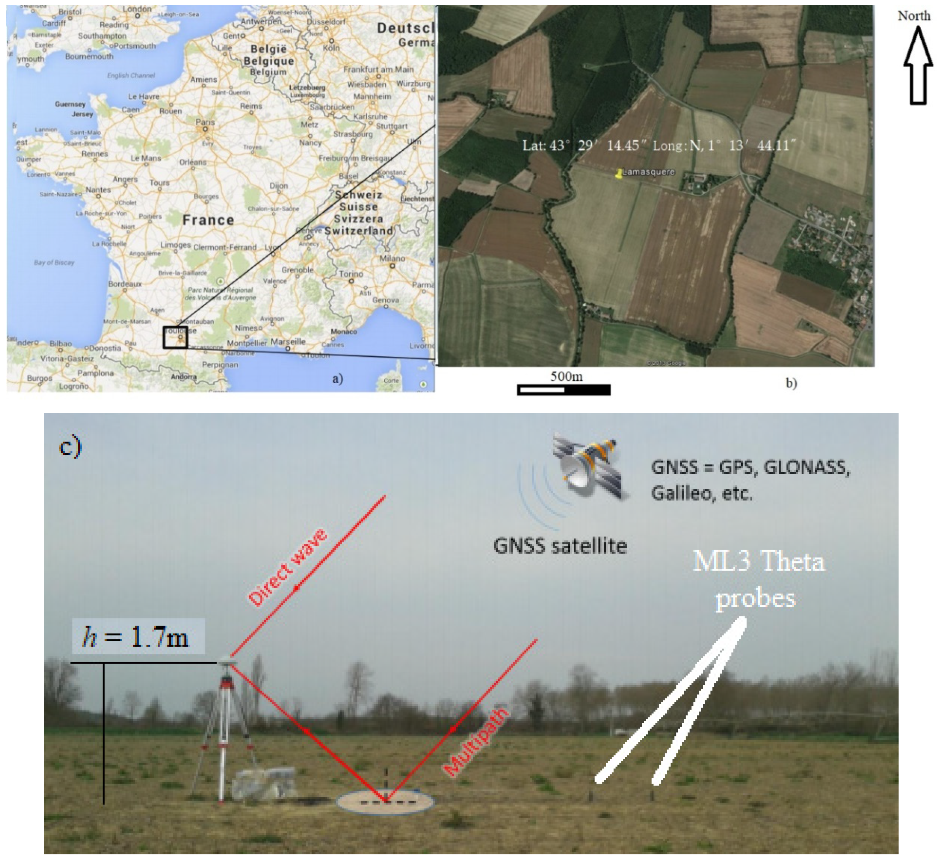
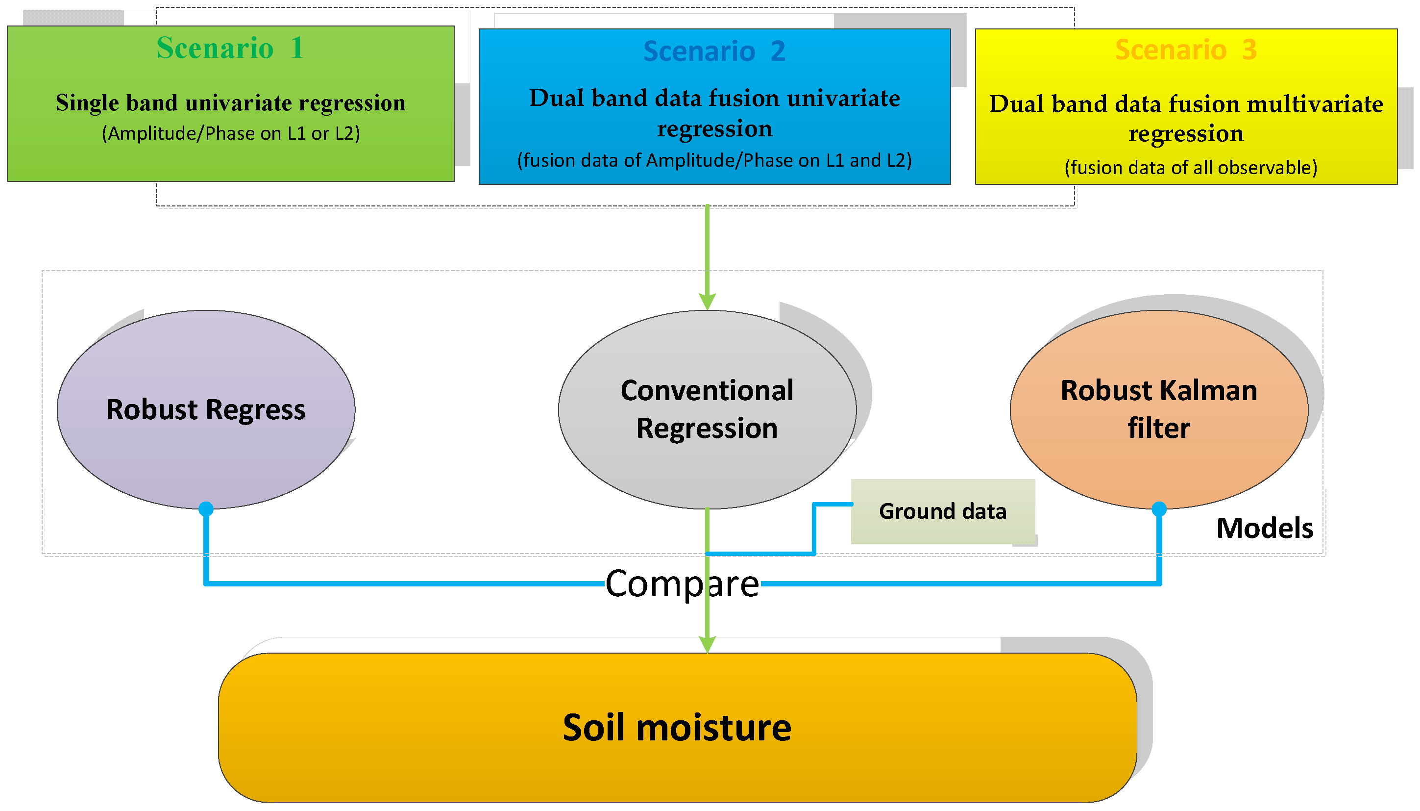
This article aims to examine and evaluate the potential of data fusion algorithms for GNSS-R applications. First, an author-proposed robust regression model will be introduced, as well as an optimized novel Robust Kalman Filter model. For validation, a dataset collected at Lamasquère (South France) will be analyzed, and the third section presents the results obtained with both robust regression model and Robust Kalman Filter model. These model retrievals are compared to (1) a classical model obtain using an empirical regression model and to (2) measurements of in situ Theta Probe ML3 sensor. The last section concludes this study by highlighting pros and cons of the different methods.
2. Methods
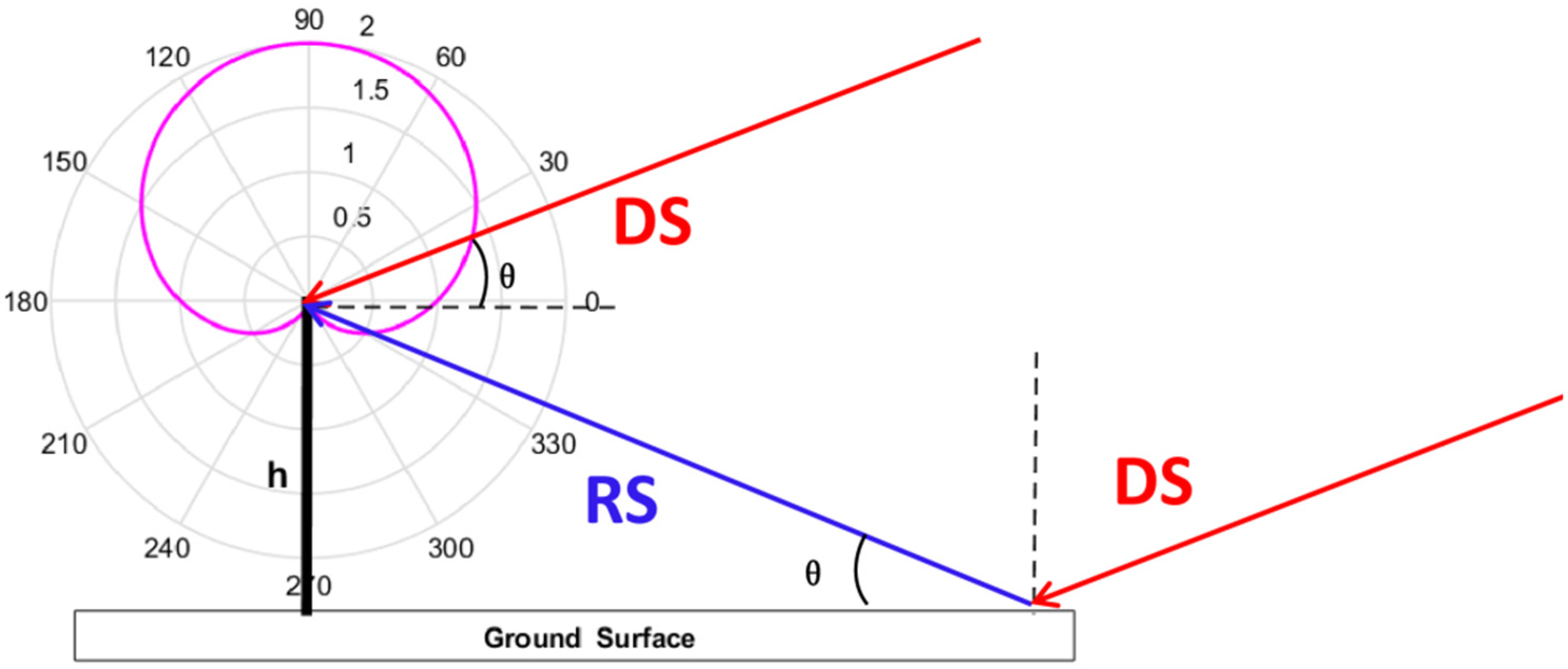
GNSS reflectometry works like Bi-static Radar systems, which consider the GNSS satellites and receiver as the radar transmitter and receiver, respectively. The main idea of GNSS-IR technology is to use a single RHCP antenna to receive both the direct and reflected signal simultaneously [
11]. In the scenario of in situ observation with low antenna height (the reflected over-path must be less than L1 C/A code wavelength ~293 m), the difference of Doppler shift between direct and reflected signal can be ignored because our application scenario is ground based measurement. If it is being used with space-borne GNSS-R receivers, the Doppler shift cannot be ignored. At the same time, if the transmit path’s difference is less than one chip, so that the two signals are coherent, then the two signals are interfering each other at the center of antenna. The scenario of interference generation is demonstrated in
Figure 1.
The reflected signal contains more RHCP component in the low elevation angle scenario, so that the interference is more significant in that case. The interference phenomenon is recorded in the SNR data stored by the geodetic GNSS receiver. Following [
16,
17], SNR can be expressed as a combination of direct and reflected signal as shown in Equation (1):
where
,
is the amplitude of direct and reflected signal, respectively,
is the phase difference between reflected and direct signal, and
is the elevation angle of GNSS satellite. When the elevation angle
changes, the phase difference
also changes, by which the oscillation in the SNR amplitude is created.
GNSS-IR technology normally utilizes geodetic receivers and antennas. In that case, the antenna’s gain pattern is designed to suppress the multipath signal coming from the bottom side for better positioning accuracy, i.e., the amplitude of SNR is mainly contributed by the direct signal (see antenna gain pattern,
Figure 1).
Supposing
is the difference between transmit paths of the reflected signal and direct signal, then
can be expressed as Equation (2):
where
is the effective height of the antenna, which refers to the distance from antenna phase center to the reflecting plane, and
is the wavelength of GNSS carrier wave.
Due to the microwave that penetrates the soil a few centimeters or decimeters (depending on the ground composition and the soil moisture) when reflected by soil surface, the reflecting plane is beneath the soil surface, so the effective antenna height varies in a range of few centimeters/decimeters with respect to the soil moisture, a key parameter in determining the penetration depth of the microwave. As the moisture usually does not change much in a few hours without precipitation, the effective antenna height can be treated as a constant to simplify the analysis.
The modified oscillation frequency can be derived by Equation (3):
For soil moisture measurement the direct signal is not of interest and typically can be removed by a second-order polynomial fitting and then derive the reflected component only, which refers to the multipath component that can be expressed by Equation (4):
where
is the dielectric constant of soil,
and
are the amplitude and phase of multipath oscillation, respectively, and
is the effective antenna height. Typical data processing method is deriving the frequency
and
by using Lomb–Scargle Spectral Analysis (LSSA), and then deriving
and
by using least mean square estimation, which corresponds to a conventional empirical model used to retrieve soil moisture.
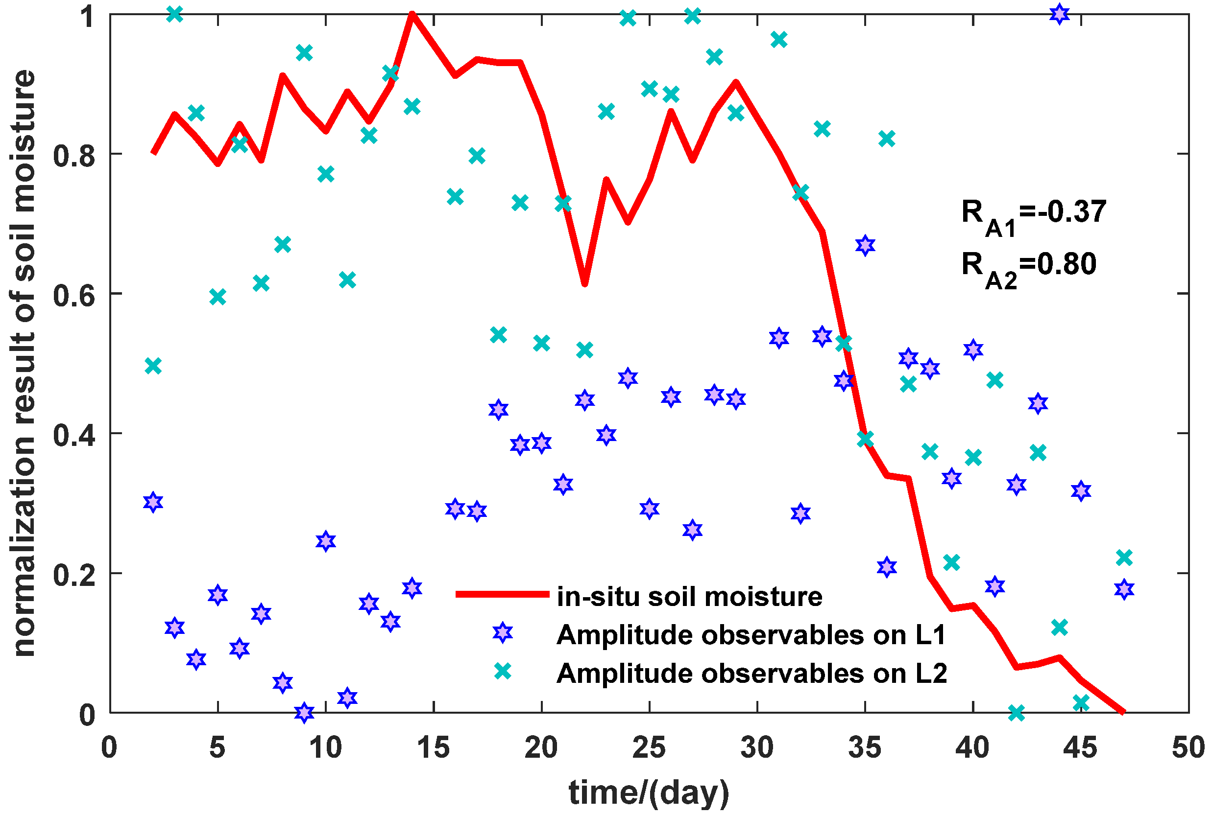
Existing studies show that normally
and
have higher correlation to soil moisture than
and
[
13,
14], so in this study we use
and
to build soil moisture inversion models. Here, we define
jth day amplitude and phase observable on L
k band as
,
(
k = (1, 2)), and then the observables’ time series vectors are
,
which are constituted by daily observables
,
, respectively. In the same way the soil moisture time series vector can be defined as
which is constituted by daily soil moisture
. In general, a GNSS-IR soil moisture retrieve model is a map function from
,
to
.
In this section, the conventional linear regression model and an author-proposed robust regression model will be introduced. Furthermore, a novel Kalman Filter model will be proposed for soil moisture inversion.
2.1. Conventional Linear Regression Soil Moisture Inversion Model
The general idea of conventional linear regression is to build a map from independent variable to dependent variable matrix, as shown as Equation (5):
where
is different coefficients being calculated for each satellite at each frequency band and
is the residual vector.
is the soil moisture time series for the whole measuring period.
is observation or its combination.
In this study we use three different strategies to make the map for GNSS-IR linear regression.
In the first strategy, we used a single-band univariate linear regression. In this case, is the single vector or . In the second strategy we used dual-bands data fusion univariate linear regression; in this case we can define two matrices , and can be either or . In the last strategy we used dual-bands data fusion multivariate linear regression. In this case we build a joint observable matrix .
In the classical process of linear regression, the least mean square method is generally used to determine and , but the disturbance of outlier noise cannot be effectively eliminated. Therefore, a robust regression model and a Robust Kalman Filter model are proposed to solve this issue.
2.2. Robust Regression Soil Moisture Inversion Model
In thesis [
33], the authors proposed a robust regression soil moisture inversion model (in Chinese). For convenience, we present now a brief description of this method in this study.
Massive studies and experimental campaigns show that the soil moisture has a near-linear relation to the observables of GNSS SNR multipath oscillation. Regression is a statistical method to build the relationship between the independent variables and the dependent variables. Robust regression is a proper algorithm to suppress the effect of the environmental noise and the thermal noise induced by GNSS receiver and antenna.
The general form of regression model is shown as Equation (5) in
Section 2.1. The residual vector
of the equation includes the constant bias of the linear regression function and also random noise.
The concept of robust regression is based on M-estimate by utilizing the Iterative Reweighed Least Squares (IRLS) method for regression coefficient estimating [
34].
A function
is defined as Equation (6):
where
is the Huber robust error function defined as Equation (7):
where
is harmonic coefficient, which generally is an empirical value. According to article [
35], when
is set to 1.345 the regression can achieve 95% efficiency with high robustness, and this value is also the default value of Matlab function robustfit, so in this study we also set
is to 1.345.
Then, the regression problem turns to an M optimization problem defined as Equation (8) for each frequency:
when
is minimalized,
, then Equation (9) is denoted:
where
, then Equation (10) is denoted:
For achieving higher robustness, a scaled estimation value
for each satellite is introduced to standardize the residuals. Following [
34], we obtain Equation (11):
where 0.6745 is median absolute deviation proposed by Hample [
36] to guarantee the unbiased estimation under normal distribution, and
is the for denoting the median absolute deviation. Therefore, we can normalize the residuals as Equation (12):
The weight of the observation on
jth day can be defined as Equation (13):
Then, we can obtain the iteration formulation of robust regression defined as Equation (14):
The main idea of the robust regression model is to assert different weights for different points depending on its residual—the smaller the residual of one point, the greater weight it will have. Then, the weights are optimized by iterating a weighted algorithm for 15 times and the first three observables are not used.
2.3. Robust Kalman Filter Soil Moisture Inversion Model
In our second model we developed a processing chain using a Kalman Filter. The idea of a Kalman Filter is to use recursion of input and output values to calculate and update by least mean square error estimation of the state. In this section we establish the state equation and observation equation. Then, we need to ameliorate the observation equation using the Huber-M estimation method. The standard Kalman Filter model assumes the true state at time
is evolved from the states at time
[
26], as shown in Equation (15). At time
, daily soil moisture
of the true state
(
,
) is made as Equation (16):
where
is the state transition matrix which is applied to the previous state
;
is the process noise with a value of zero which is assumed to be drawn from a zero-mean multivariate Gaussian distribution
, with covariance
.
is the observation model which maps the true state space into the observing space and is the observation noise which is assumed to be zero-mean Gaussian white noise with covariance .
Here is given a recursive process. We estimate the state at time j through the state at time j − 1, then calculate the error correlation matrix and Kalman gain , update the state variable, and then output . The recursive algorithm of Kalman Filter is demonstrated as follows.
First, set both the
and
to be an identity matrix as the entrance of the recursive algorithm. Then, calculate each state
at time
predicted by state
at time
defined as Equation (17):
Calculate the error covariance matrix that is between predicted and true values defined as Equation (18):
According to Equation (18), Kalman gain can be computed as Equation (19):
Equations (17) and (19) are used to calculate the estimated value of
at time
, defined as Equation (20):
Then, compute the error covariance matrix that is between estimated and true values defined as Equation (21):
where
is the identity matrix.
To obtain the optimal Kalman gain, the error covariance matrix further simplifies to Equation (22):
Normally, Kalman Filter is more effective for suppressing Gaussian distributed noise. Otherwise, the robustness will be impacted. Therefore, we try to use the Huber-M estimation described in
Section 2.2 to reconstitute the observables for improving the robustness. The relationship between state truth value
and its predicted value
at time
j is shown as Equation (23):
where
is the error of prediction. A linear regression model is constructed by combining Equation (16) as Equation (24):
Then, we define Equation (25):
Combined with Equation (2), we can define Equation (26):
By combining Equation (13), iteration
is solved as described in Equation (27):
where
is the transpose of
,
is the matrix of weight, and
is the observation for true value
.
The result of the
th iteration as Equation (28):
At the end of the iteration, the variance is obtained as Equation (29):
Introducing Equations (28) and (29) above results into the updating of the observations in Equations (20) and (22), and the Huber-M estimation Robust Kalman Filter algorithm is computed.
4. Analysis and Discussion
It has been demonstrated that GNSS-IR has the ability to retrieve land surface parameters, and especially the observable of soil moisture. After K. Larson first retrieved soil moisture from GPS SNR data [
14], massive studies have developed models for GNSS-IR soil moisture inversion. Although most studies focus on low elevation angles, in article [
37] which was mentioned above, the authors take the pseudo-dynamic of the surface into account and obtain a significantly improved and also utilized signal with high elevation angles. How to apply the Robust Kalman Filter model with signal of high elevation angles is a main interest in future work.
In the experimental campaign of Lamasquère, the land is bare soil, but how to eliminate the impact of vegetation is also important. In article [
38], the author proposed a multivariate adaptive regression spline method, considering the impact of the vegetation moisture content, with a correlation coefficient of 0.916 and a root-mean-squared error of 0.021 m
3/m
3. In article [
39], the authors performed a 15-month observation which covered an entire growing cycle by two antennas and developed an inversion model on GPS L2C and L5 SNR, achieving a precision of 0.035 m
3/m
3 for the whole meadow growing cycle, and of 0.018 m
3/m
3 after grass cutting.
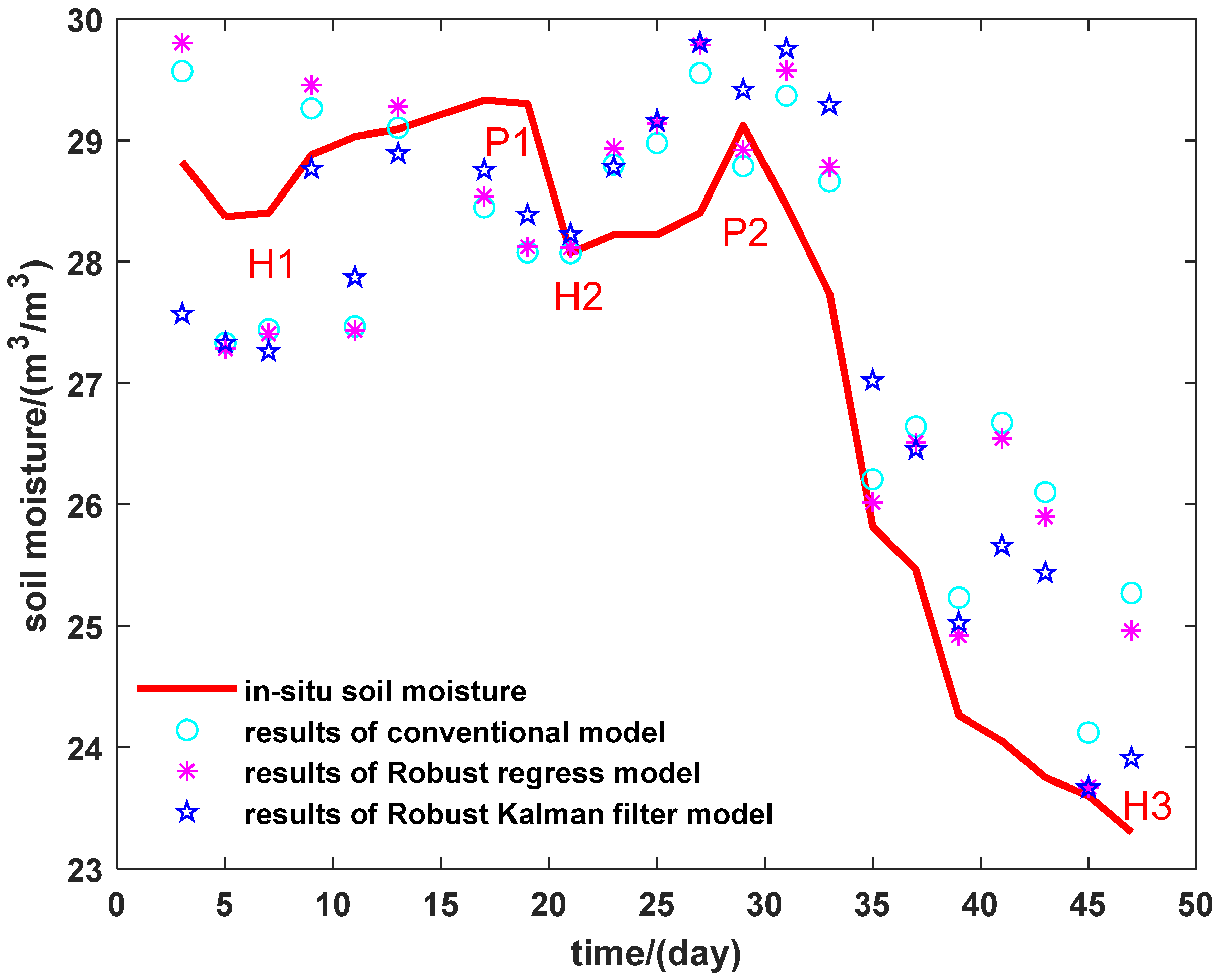
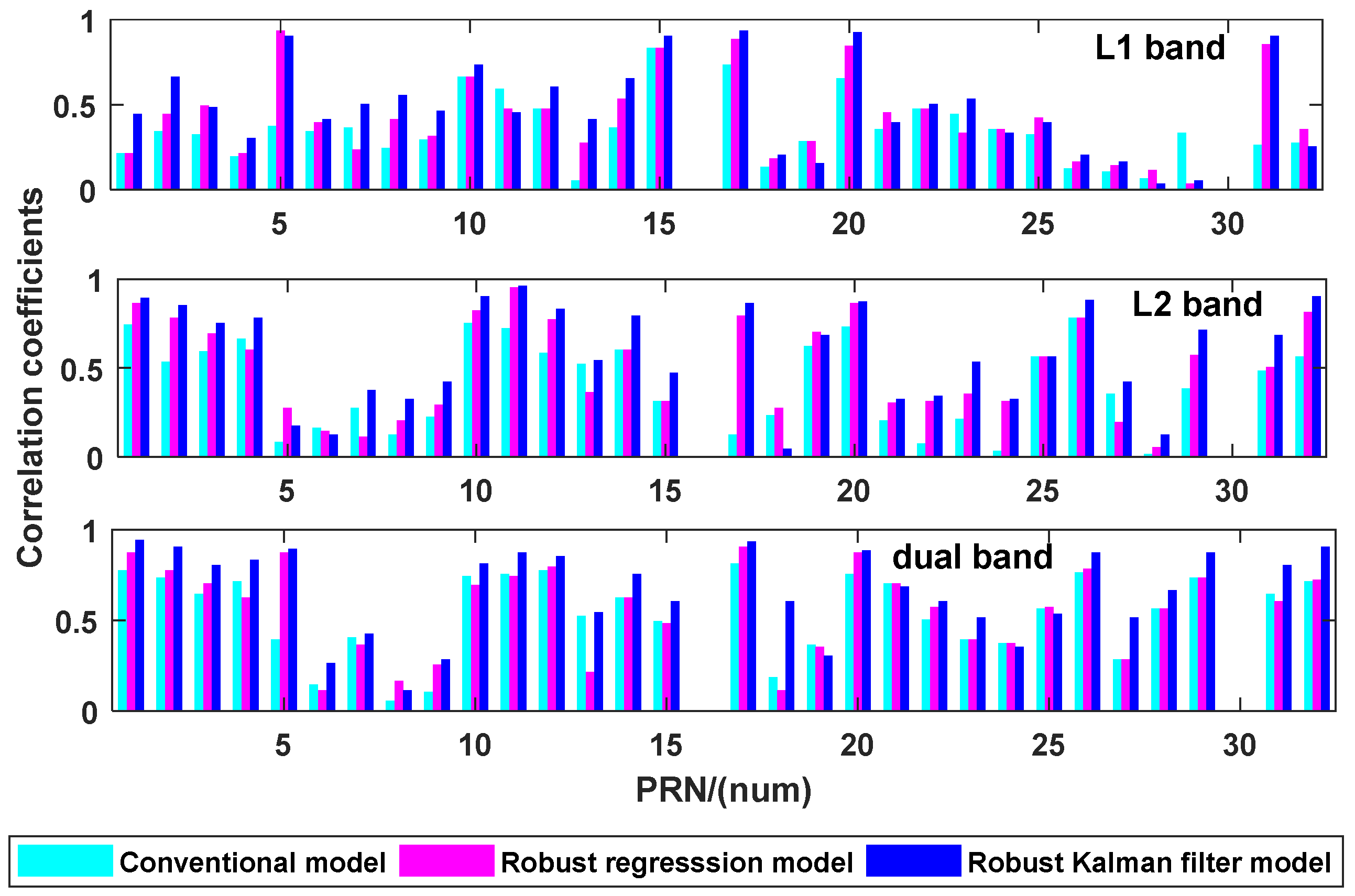
For every model, the correlation coefficients are calculated for each satellite on each band or dual-band combination as
Figure 11. Satellites in which correlation coefficients are over 0.5 are considered as effective cases.
Compared with the conventional model, the robust regression model increases on average 28.77% for L1, 18.33% for L2 and 5% for dual-band. The correlation coefficient of the Robust Kalman Filter model increases on average 32.33% for L1, 28.14% for L2 and 19.10% for dual-band. As the statistical data shows, the Robust Kalman Filter model achieves the highest precision.
The correlation coefficients of the three models show that the Robust Kalman Filter model gives a better correlation than regression models, except for satellites PRN 6, 7, 8, 9, 19 and 24, for which the correlation coefficient is very weak, reflecting a non-correlation (R < 0.5). For demonstration, we counted the number of effective satellites for all the methods, as shown in
Table 1.
There are 7 satellites for the robust regression model and 4 for conventional regression model on the L1 band, but the Robust Kalman Filter model has 13 satellites for soil moisture inversion. On the other hand, data fusion has also had a positive impact on the increase in the number of effective satellites. If we compare the results of the conventional method for dual-band and single-band, the correlation coefficient of the L1 band with an average increment is 48.66% and a maximum grow of 90.38%. Meanwhile, the correlation coefficient of L2 with an average increment is 26.93% and a maximum grow of 98.21%. For the robust regression model, the correlation coefficient of the L1 band with an average increment is 34.45% and a maximum grow of 80.36%. Meanwhile the correlation coefficient of L2 with an average increment is 14.06% and a maximum grow of 91.07%. The correlation coefficient of the Robust Kalman Filter model on the L1 band with an average increment is 34.80% and a maximum grow of 95.45%. Meanwhile, the correlation coefficient of L2 with an average increment is 18.50% and a maximum grow of 93.33%.
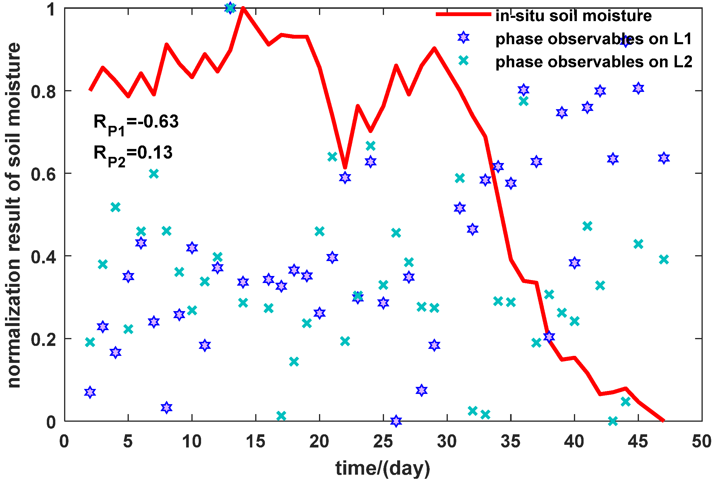
Then, we analyzed the correlation between the phase observable and in situ soil moisture as shown in
Figure 12.
The correlation of phase is not better than amplitude and there are few satellites effective for soil moisture estimation. However, we can see that there are some satellites which are not effective for conventional methods but effective for robust regression and Robust Kalman Filter method. It shows both the robust regression and Robust Kalman Filter models are capable of increasing the number of effective satellites, such as PRN5 and PRN26 for the L1 band, and PRN3 and PRN14 for the L2 band. The figure also shows that the dual-band data fusion method makes improvement of correlation between the phase observable and in situ soil moisture.
Compared with the conventional model, the robust regression model increased by an average of 24.59% for L1, 35.22% for L2 and 24.63% for dual-band. The correlation coefficient of the Robust Kalman Filter model increased by an average of 33.96% on L1, 43.92% on L2 and 35.29% for dual-band. The Robust Kalman Filter can greatly improve the inversion accuracy of the model regardless of single frequency or dual-band fusion.
If we look the precision of the three models, i.e., correlation coefficients, one can see that the Robust Kalman Filter model gives a better correlation than regression models, except for satellites PRN 6, 9, 10, 12, 18, 19, 21, 22, 23 and 29, where the correlation coefficient is very weak and reflects a non-correlation (R < 0.5). For demonstration, we counted the number of effective satellites for all the methods, as shown
Table 2.
The table shows that there are more effective satellites on the L1 band than L2 band and the dual-band data fusion also has a positive impact for increasing the number of effective satellites.
If we compare the results of the conventional method for dual-band and single-band, the correlation coefficient of the L1 band with an average increment is 25.68% and a maximum grow of 95.45%. Meanwhile, the correlation coefficient of L2 with an average increment is 36.46% for L2 and a maximum grow of 93.24%. For the robust regression model, the correlation coefficient of the L1 band with an average increment is 17.38% and a maximum grow of 93.84%. Meanwhile, the correlation coefficient of L2 with an average increment is 28.60% and a maximum grow of 98.75%. The correlation coefficient of the Robust Kalman Filter model on the L1 band with an average increment is 19.74% and a maximum grow of 98.61%. Meanwhile, the correlation coefficient of L2 with an average increment is 31.76% and a maximum grow of 97.67%.
Compared with the correlation coefficient of the amplitude observable, dual-frequency fusion has a better effect on the L2 band and a greater improvement. However, the amplitude is reversed.
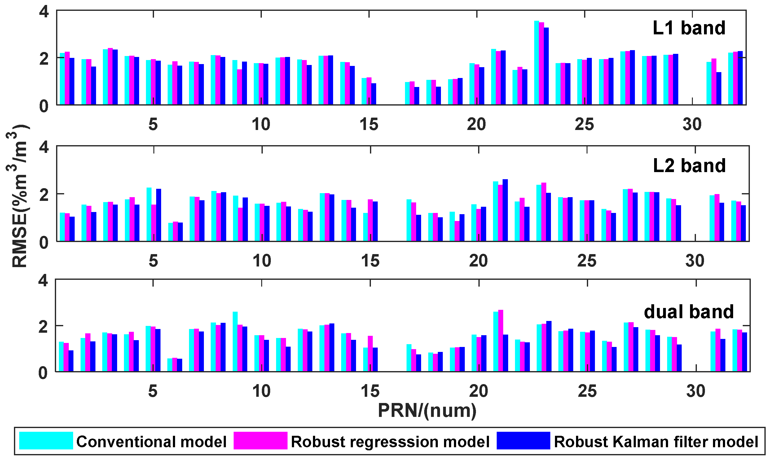
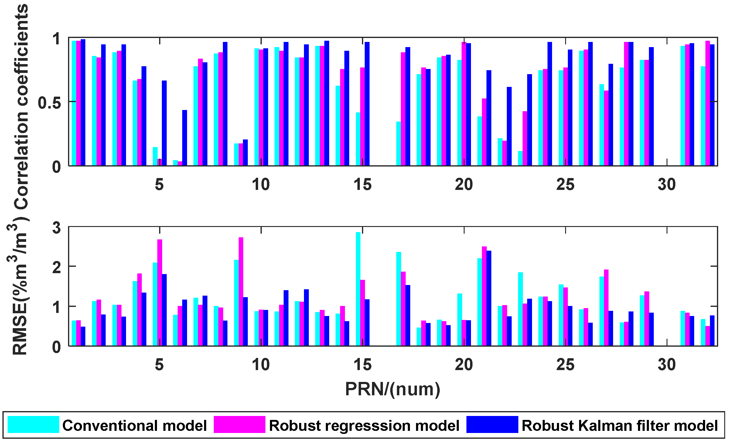
For every model, the root-mean-squared error (RMSE) is also calculated for each satellite on each band or dual band combination. The results are shown in
Figure 13 and
Figure 14. All the discussion for RMSE is based on valid satellites defined in line 498~499.
First, we discuss the results with amplitude. Compared to the conventional method, the RMSE of the robust regression model decreases by an average of 2.54% on L1 and 2.81% on L2, meanwhile the RMSE of the Robust Kalman Filter model decreases by an average of 10.19% on L1 and 12.39% on L2. Over half of the satellites’ RMSE are between 1% m3/m3 and 2% m3/m3 for the Robust Kalman Filter model.
After dual-band data fusion, the RMSE of the conventional model decreases 12.10% more than L1 and 3.46% more than L2. The RMSE of robust regression model decreases 14.30% more than L1 and 0.72% more than L2. The RMSE of the Robust Kalman Filter model decreases 18.23% more than L1 and 7.28% more than L2. As the statistical data show, the Robust Kalman Filter model demonstrates the highest precision.
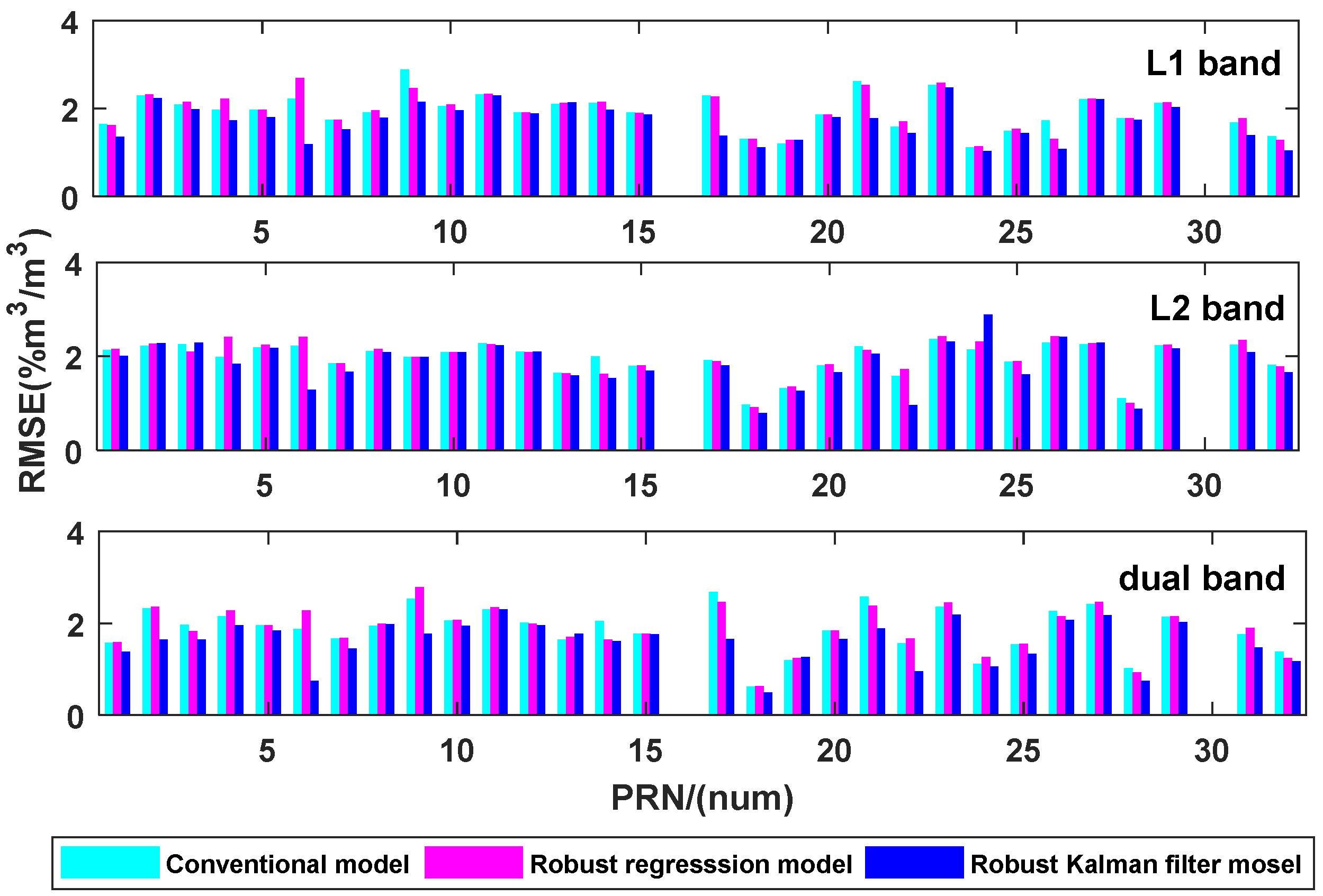
Moreover, we discuss the results with phase. Compared to the conventional method, the RMSE of the robust regression model decreases by an average of 1.32% on L1 and 6.11% on L2, meanwhile the RMSE of the Robust Kalman Filter model decreases by an average of 11.49% on L1 and 8.87% on L2. Over half of satellites’ RMSE are between 1% m3/m3 and 2% m3/m3 for the Robust Kalman Filter model.
After dual-band data fusion, the RMSE of conventional model decreases 5.45% more than L1 and 46.5% more than L2. The RMSE of the robust regression model decreases 2.08% more than L1 and 45.01% more than L2. The RMSE of the Robust Kalman Filter model decreases 1.24% more than L1 and 47.18% more than L2. As the statistical data show, the Robust Kalman Filter model demonstrates the highest precision.
In the end, we discuss dual-band multivariate data fusion models. The correlation coefficients and RMSE are shown in
Figure 15.
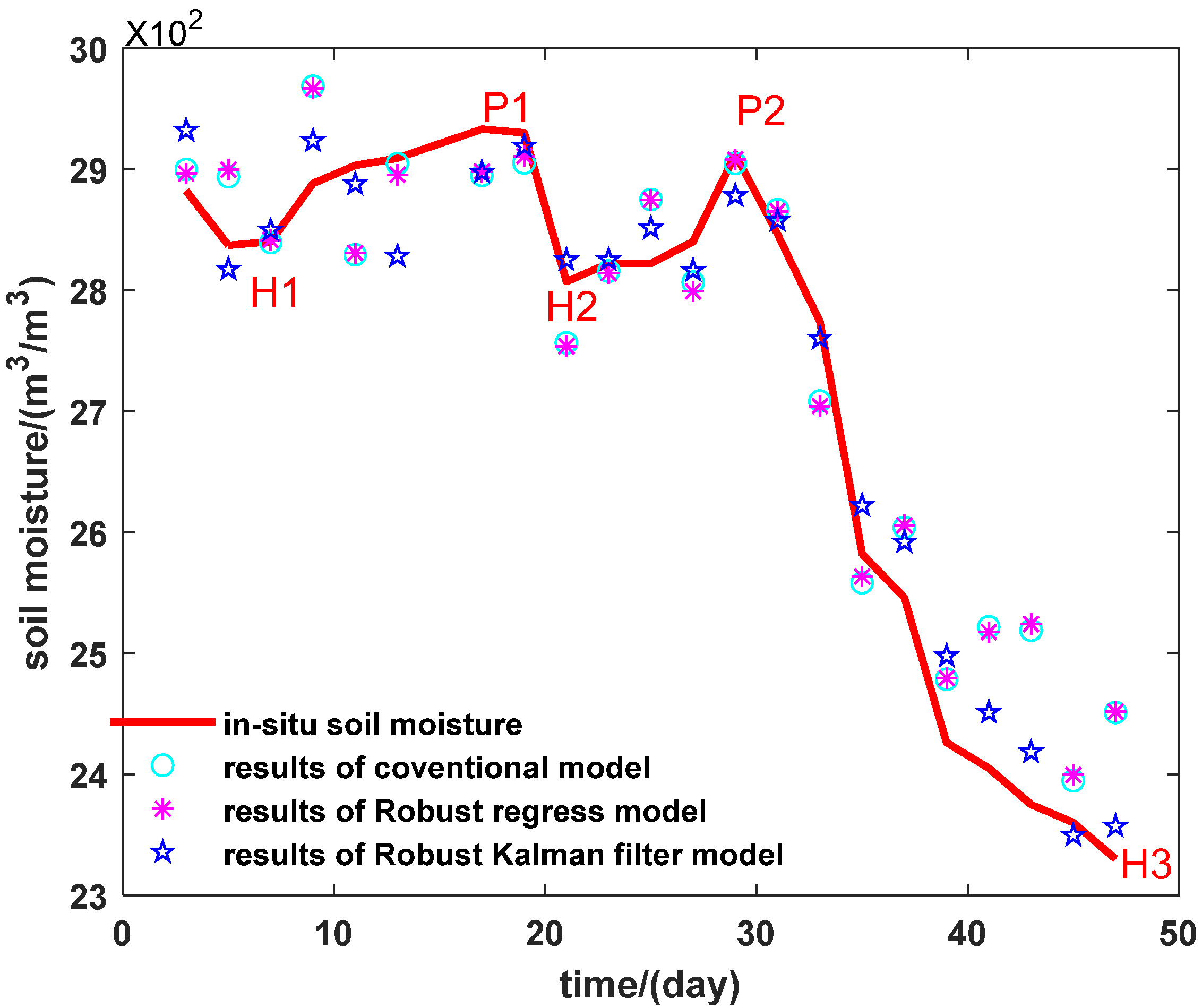
As demonstrated in
Figure 15, the correlation between the inverted and the in situ soil moisture has been significantly enhanced for all the models, regardless of single-band or dual-band data fusion approach. The conventional model has 22 effective satellites un-der the multivariate fusion scenario, while the robust regression and Robust Kalman Filter methods have 25 and 28 satellites, respectively, by which means we have more effective satellites to estimate soil moisture than univariate models.
Compared with the results of the univariate models, the correlation coefficient of dual-band data fusion multivariate conventional method self-improves for all the GPS satellites with an average increase of 44.97% for phase and an average increase of 29.43% for amplitude; meanwhile, the RMSE decreases by an average of 37.00% for amplitude. The correlation coefficient of dual-band data fusion multivariate robust regression model self-improves with an average increase of 29.43%, meanwhile the RMSE decreases for all satellites with an average reduction of 29.42% for amplitude. The correlation coefficient of dual-band data fusion multivariate Robust Kalman Filter self-improves with an average increase of 20.7%, meanwhile the RMSE decreases for all satellites with an average reduction of 31.42%.


 ,
, 


