
Direct Aerial Visual Geolocalization Using Deep Neural Networks

1
Department of Industrial Engineering, University of Arkansas, Fayetteville, AR 72701, USA
2
Department of Geosciences, University of Arkansas, Fayetteville, AR 72701, USA
*
Author to whom correspondence should be addressed.
Remote Sens. 2021, 13(19), 4017; https://0-doi-org.brum.beds.ac.uk/10.3390/rs13194017
Submission received: 31 August 2021
/
Revised: 27 September 2021
/
Accepted: 28 September 2021
/
Published: 8 October 2021
(This article belongs to the Special Issue Computer Vision and Deep Learning for Remote Sensing Applications)
Abstract
:Unmanned aerial vehicles (UAVs) must keep track of their location in order to maintain flight plans. Currently, this task is almost entirely performed by a combination of Inertial Measurement Units (IMUs) and reference to GNSS (Global Navigation Satellite System). Navigation by GNSS, however, is not always reliable, due to various causes both natural (reflection and blockage from objects, technical fault, inclement weather) and artificial (GPS spoofing and denial). In such GPS-denied situations, it is desirable to have additional methods for aerial geolocalization. One such method is visual geolocalization, where aircraft use their ground facing cameras to localize and navigate. The state of the art in many ground-level image processing tasks involve the use of Convolutional Neural Networks (CNNs). We present here a study of how effectively a modern CNN designed for visual classification can be applied to the problem of Absolute Visual Geolocalization (AVL, localization without a prior location estimate). An Xception based architecture is trained from scratch over a >1000 km2 section of Washington County, Arkansas to directly regress latitude and longitude from images from different orthorectified high-altitude survey flights. It achieves average localization accuracy on unseen image sets over the same region from different years and seasons with as low as 115 m average error, which localizes to 0.004% of the training area, or about 8% of the width of the 1.5 × 1.5 km input image. This demonstrates that CNNs are expressive enough to encode robust landscape information for geolocalization over large geographic areas. Furthermore, discussed are methods of providing uncertainty for CNN regression outputs, and future areas of potential improvement for use of deep neural networks in visual geolocalization.

1. Introduction
Pilotage or piloting is the practice of using vision to navigate an aircraft, usually by reference to terrain and landmarks. This is in contrast to flying by instrument. Modern aircraft instruments enable navigation even in the absence of vision. However, vision and visual flight remains immensely valuable to pilots when it is available, both in improving navigation quality and as a check against instrument error. Despite possessing cameras, automated drones are not currently capable of navigating using vision, even in clear weather conditions. Thus, a valuable source of navigation capability and backup instrumentation is currently not being utilized. This is of particular concern in the context of security and reliability, when external navigational aids may not always be available or reliable [1].
Navigating by sight is a complex task that requires the ability to recognize and contextualize terrain features from images under a wide variety of conditions. A recent review of the field by Couturier and Akhloufi [2] divides current approaches into two broad categories: Relative Visual Localization (RVL or frame to frame localization), which aims to update location by calculating movement when comparing one image frame to the next, and Absolute Visual Localization (AVL or frame to reference localization), which aims to determine location by comparing UAV/aircraft imagery to trusted georeferenced imagery, commonly from high-altitude survey flights or satellites. Of the two approaches, AVL has the notable advantage of being free from drift while RVL approaches tend to be more accurate than AVL approaches over short distances. Over longer distances, errors compound, as each error in estimating movement from the last frame adds to the error in estimating current location. AVL, however, can provide estimates of location that are independent of prior estimates. AVL, then, can be used as a complement to RVL. RVL provides high accuracy over short distances, while AVL provides periodic, independent estimates of location to prevent drift. This is similar to how GPS and IMUs work together, where IMUs provide high accuracy over short distances, while GPS provides periodic independent location information to prevent drift. Preventing drift is particularly important for long duration flights over large distances, typically made at high altitude. However, most prior work on AVL has focused on lower altitude flights by small UAVs, highlighting a need for investigation of AVL using higher altitude imagery.
Since AVL involves image processing, it is natural to investigate how the current state of the art in ground level image processing techniques performs when applied to this task. One of the most successful modern techniques for complex visual processing tasks is the Convolutional Neural Network (CNN). CNNs are very effective at learning complex relationships between input images and outputs. Furthermore, although the computational and memory resources needed to train a CNN are high, a fully trained model can be deployed at a considerably reduced cost, which is a desirable feature for UAVs whose computational resources may be limited.
Many frame-to-reference AVL approaches require the aerial platform to locally store reference imagery which must be retrieved during localization, meaning that storage and computational costs rapidly increase with the area of flight operation. Additionally, such AVL approaches that seek to increase accuracy/robustness by comparing to multiple reference data sets increase their storage and computational costs proportionally. In contrast, a pure neural network approach only requires the storage of the model parameters, and does not need to scale with the number of data sets used during training, and does not directly scale with the size of the ROI (larger ROIs will require larger networks with more parameters to encode information about locations in the ROI. It would take more parameters to encode a state than a county. However, because neural networks are known to be effective at efficiently encoding data (for example, in autoencoders), the size of the network needed to localize over a given ROI should not be directly proportional to the ROI’s area). Finally, although neural networks have large requirements for data and computation during training, the speed of inference on a trained neural network is quick. This makes a pure neural network approach highly desirable if it can achieve useful accuracy over a large area. This paper aims to address the question of how effectively a modern CNN architecture that has been successfully used on ground-level imagery tasks can be repurposed for AVL.
When making neural networks for tasks involving recognizing objects at the ground level, there exist many high-quality pretrained models that can be used as a starting point. Unfortunately, there do not currently exist large, pretrained deep learning models for aerial imagery feature detection. In contrast to most prior work in the field (see Related Work section for details), we fully train our own model. This requires a large and varied data set. Although large quantities of location-tagged aerial imagery exist, organizing and processing them for use in training a neural network remains an ongoing challenge. For this study, publicly available high-altitude images were used. Images are precropped and downscaled to allow for input into a CNN. Additional random crops augment the training data. One of the challenges of AVL is that the photographic properties of the input may vary considerably due to factors such as time of day, season, year, weather, and the properties of the camera used. This study therefore trains and tests on different image sources that vary by as many of these factors as possible.
Several configurations of CNNs were trained from scratch to regress latitude and longitude coordinates from high-altitude photographs (covering 1.5 × 1.5 km each) over the region of interest (ROI, the selected area within which localization was assessed), a 32.2 by 32.2 km section of Washington County encompassing urban, suburban, and rural areas. The best performing architecture, Xception [3], was investigated further. An investigation into the use of probability distribution parameters as outputs in order to quantify model uncertainty was performed. The final models were trained on 12 data sets and tested on a 13th, with a separate model being trained with each data set acting as a holdout set to act as cross-validation. Performance was robust across all cross-validation training runs, and performance was high relative to the area of the ROI and size of the input images, where average errors were as low as 0.004% of the ROI’s area and 8% of input image width, respectively. Future directions to improve CNN performance on this task, and better incorporate them into overall UAV navigation models, are discussed.
Related Works
Visual localization can be split into two broad categories: relative visual localization (RVL) or frame-to-frame localization, and absolute visual localizationn (AVL) or frame-to-reference localization. Although this paper is addressing the problem of AVL, RVL is the more mature field and the field of AVL has developed primarily out of a need to address drift in RVL approaches. Because RVL provides a location relative to the last location estimate, error inevitably compounds no matter how accurate the technique (unless the error is zero—a very high bar to cross!). Thus, even the most accurate RVL techniques have unbounded error over long enough timescales. In application, AVL is best used together with RVL, with RVL providing high accuracy over short distances and AVL preventing drift from becoming unbounded. Additionally, RVL can only provide relative position updates - it can not localize when there is no initial estimate of position, while AVL can.
The most straightforward type of RVL is visual odometry (VO) [4]. VO compares the current and prior observation, compares them, and then determines the movement of the platform based on differences. VO approaches evolved out of feature-based detection algorithms such as SIFT [5] (Scale-invariant Feature Transform), where certain features, crafted to be robust to image transformations caused by camera pose, are extracted from each image and then matched across images. The difference in the locations and orientations of these features within each image can then be used to estimate camera movement. Feature extraction and matching is computationally intensive, leading to interest in VO methods that do not use feature extraction (see [6] for an example). Additionally, some approaches now also incorporate additional information from IMUs to increase accuracy, an approach called Visual Inertial Odometry [7].
Because VO updates position from prior estimates, it is susceptible to drift over time. If the aircraft loops over prior locations (loop closure), then if the previously visited location is recognized the aircraft can reconcile its current and past location estimates, eliminating drift. This is approach taken in Simultaneous-Localization Furthermore, Matching (SLAM) [8], where a map of prior visited locations is constructed simultaneously with location estimation. However, in the absence of loop closures (such as in straight-line flight), or if it fails to recognize a prior location, SLAM is still susceptible to drift. Additionally, SLAM requires additional computational resources to store and query its map of prior locations - and this cost increases over operation time as the number of prior locations grows. Thus, although effective, SLAM does not solve the problem of location drift in all situations, highlighting the need for AVL approaches. In contrast to RVL, which updates position based on a prior estimate, AVL compares the operational imagery during flight to a trusted reference to produce a location estimate. Since each comparison to the reference is made independently, each location estimate is independent of previous estimates and is not susceptible to compounding drift.
Couturier and Akhloufi recently published an excellent review of AVL [2] which covers much of the recent publications in the field. From this review, it is seen that the most popular and currently most successful AVL methods use template or feature points matching, with only a minority opting to use deep learning techniques, and even then often only using deep learning techniques as a supplement to another matching technique. This is despite deep learning being the leading method in various ground-based tasks, including analogous problems such as self-driving cars. Neural networks are also being successfully applied to the related problem of cross-view geolocation, where ground level pictures of locations must be matched to aerial pictures of the same location (see for example Hu et al. [9]).
There are two major difficulties facing researchers attempting to leverage deep learning on aerial photographs: lack of existing models, and difficulty in obtaining sufficient train/test data. Although it is still possible to use the early layers of models trained on ground level imagery tasks, it is likely that the filters learned when training on ground level imagery are inefficient when applied to aerial imagery, especially high-altitude imagery, due to the vast difference in image scale and perspective. Nonetheless, because of the difficulties in training a deep model from scratch, most papers using them to-date have opted to fine-tune existing pre-trained ground-level models [see, e.g., [10,11,12,13]]. Unlike our approach, none of these works attempt to directly determine location using a deep model, but instead use neural networks as steps along a template or segment matching pipeline. Thus, the potential of a purely CNN based AVL procedure remains unknown.
Additionally, because of the large computational cost of matching over a large area, many models employ some level of search space reduction such as a sliding window [13] or constant registration of the current position [12]. This presents a problem if the error in the estimate of position ever becomes too large: the reduced search space may no longer include the true position. In other words, these systems can suppress small-scale drift, but are still susceptible to drift resulting from larger errors. They also can not localize without some estimate of initial position. Thus, they are susceptible to outlier estimates, system memory failure, and are unsuitable for recovering from an extended navigation blackout (e.g., flying through an extended fogbank or cloud in a GPS-denied environment).
Schleiss et al. [14] fully train a generative adversarial network, but use this to convert input images into a semantically segmented (to roads, buildings, and none) map-like image to template match to an also segmented reference map (in this case, from OpenStreetMap, OSM). They do not employ any search space reduction, but their test area is only 560 m long and 680 m wide. Because their template matching technique uses a sliding window approach, it would likely require some form of search space reduction to remain computationally feasible over a larger area. Notably, they train and test on different (though geographically nearby) regions. The ability for this technique to generalize outside of the trained area is a considerable benefit, as it means that it is not necessary to train a model over the operational area specifically. However, the fact that the model must segment the image to match to a specific reference map creates two possible issues. First, as demonstrated in the paper, the model cannot differentiate areas with limited texture of the selected semantic categories (for example, a forest with no structures or roads). Second, although one can apply this technique to regions not trained on, the technique does requires an accurate reference map segmented in the same manner as the model was trained on. In this case, the model could only be applied to where OSM has an accurate segmentation of the local terrain already available.
To our knowledge, only one other published work on AVL to-date has trained a deep CNN from scratch for direct regression AVL. Marcu et al. [15] trained a multi-stage multi-task architecture for simultaneous geolocalization and semantic segmentation. Their best approach uses a model that treats AVL as an image segmentation problem, and combines this with a simultaneous semantic segmentation that is then used to fine tune the image correspondence by matching identified roads. They also train one branch of their network for direct regression of latitude and longitude. However, the output of the direct regression branch is not the focus of their paper, and results are only reported in a single histogram (thus average error is not known). Additionally, although different train and test images are used, they appear to be from a common source and therefore have similar photographic qualities. Learning to identify locations across multiple photographic sources which may differ in time of day, season, year, and photographic platform is a considerably more difficult challenge.
2. Methods and Results
2.1. Data Choice and Processing
An effective deep learning approach to AVL should be robust to factors such as time of day, season, year, altitude, weather, angle of approach, and the camera used, maintaining accuracy under as many different conditions as possible. Producing robustness to these factors in a neural network requires large, high quality input data that includes the full range of plausible scenarios within it. Furthermore, all of these data must be georeferenced accurate to the desired scale. Unfortunately, such data is not readily available to the public in an organized form, which has hampered research efforts in this field.
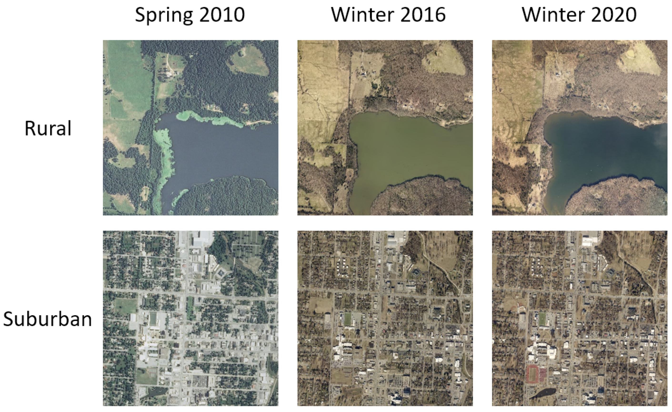
Georeferenced imagery from satellite and high-altitude survey flights, however, are readily available, and serve as a reasonable proxy to high-altitude UAV images (indeed, an increasing number of such image sets are from high-altitude UAVs). In total, 13 data sets over Washington County, Arkansas were acquired (see Appendix A for detailed information on data sets and links to source data). These data sets differ in year taken (from 2006 to 2020), season, time of day, and camera used. All image sets used are from clear weather, daytime flights due to the vast majority of georeferenced, publicly available data being of this type. The data sets are also orthorectified using a mixture of digital elevation models—some from national elevation datasets and others from elevation data produced from the aerial triangulation results. For high altitude flights this alteration is relatively minor as the photographs are already taken nearly vertical angles and the terrain effects in this area are minimal at the flown altitudes. See Figure 1 for examples of 3 × 3 km crops and how they vary between a few of the datasets.
Since the data sets did not all completely cover Washington County, a 34.2 by 34.2 km square patch included in all data sets was chosen as the ROI within which localization would be assessed. This area includes both the urban centers of Fayetteville and Springdale, as well as the suburban and rural areas around them. The presence of highly varied terrain and land use - including both developed and undeveloped areas - makes this an especially good test of our approach’s robustness to terrain character.
From each data set, 2000 3 × 3 km random crops and their locations were taken from the ROI and downsampled to 1000 × 1000 pixels for speed of image loading and manipulation. During training of the neural network, each one of these crops is randomly cropped again to 1.5 × 1.5 km and downsampled to 224 × 224 pixels. Thus, a full epoch of training exposes the network to 2000 images from each data set, each of which is at least slightly novel due to random cropping. The labels for the network are the latitude and longitude of the image centers (in implementation the upper left-hand corner location was used as the label, as this is the native format of world files. Because all images are North–South aligned, the image center is always 750 m down and to the right of the upper-left hand corner, and so determining the location of the corner also determines the location of the image center), with locations adjusted as needed during cropping, scaled first to a range between 0 and 1 using a min-max scaler. The scaling applied is such that, over the entire dataset, the minimum latitude and longitude is 0 and the maximum is 1. Since the coordinate system used during processing increases in the west–east, south–north directions, the bottom left (southwest) corner of the ROI has coordinate (0,0), and the top-right (northeast) corner has coordinate (1,1) (thus the ROI is normalized to the unit square). When adjusting labels during random crops, the flat world assumption is used, which is justified because the images are high-altitude and orthorectified vertical. This also justifies the conflation of image centers and UAV location; for a camera looking straight down they will be approximately the same. See Figure 2 for a visual overview of the image processing pipeline.
The offline initial crop and downsampling is done using bicubic interpolation, however the online resizing for loading into the neural net is done using bilinear interpolation to reduce computational time. The image crops are saved as jpegs to reduce file size. Although both resampling and jpeg compression can introduce artifacts in images, both training and test images go through the same downsampling process, so these artifacts are consistent at train and test time. Pilot runs (data not shown) showed no significant difference in final model accuracy from using different common resizing methods.
2.2. Network Architecture Selection
For initial selection of network architecture, we decided to test a variety of architectures already available in Keras [16] as built-in models (see Appendix A for detailed information on implementation and hyperparameter choice. Model references: EffNet [17], ResNet [18], VGG [19], MobileNetv2 [20], Inception [21], Xception [3]). These include many of the most successful models for various classification data sets and competitions over the last decade. Because we were only interested in comparing the models, the data set used for classification was a limited one where training and test was restricted to only one data set (ADOP2017). Furthermore, fine tuning for each architecture was minimal, so this comparison should not be taken as a final verdict on model performance. Performance is reported in mean absolute error on the x, y in the converted coordinate scheme as this test was solely intended for a preliminary model comparison. Models were given 500 epochs to train. See Appendix A for further implementation details.
Results are shown in Table 1. Based on Xception’s high performance and relatively small model size, it was selected as the model of choice for further experiments. For subsequent experiments, Xception was modified to include additional fully connected and dropout layers before the output layer in order to provide additional regularization and capacity (these modifications are similar to some of the configurations used in [3]).
2.3. Field of View Comparison
As the altitude of an aerial platform increases, the field of view, and therefore the number of features that can be seen and used to navigate, increases. However, distance also decreases the ability to resolve smaller objects, and fine features are lost. In order to investigate this tradeoff within a CNN context, different field of views for the input images were tested while holding the input size fixed at 224 × 224 pixels. At the time this experiment was performed, the data set only had 11 of the 13 data sets in it. Holdout data set was held constant as the ADOP2006 data set for comparison. Training was performed for 250 epochs.
See results in Table 2. Results are reported in normalized RMSE (NRMSE) for simple comparison. Within the range studied, it was found that increasing field of view increased performance. There is a confounding factor that due to the processing pipeline, very large fields of view had fewer unique crops (that is, cropping a greater percentage of the source image reduces the difference between crops), however, this would be expected to decrease performance due to producing less varied training data.
2.4. Loss Function Comparison
For regression tasks there are numerous loss functions available to train a neural network. Since backpropagation training of neural networks is not a straightforward optimization relative to the loss function, it is not the case that using the desired metric as a loss function will lead to the best results as measured by that metric. That is, if our desired metric is to minimize the Euclidean distance between the predicted and actual location, the loss function that produces the best model may not be the Euclidean distance itself. It is therefore necessary to investigate loss functions and empirically observe their impact on model training.
For this experiment, three loss functions were investigated. First, mean squared error, which is the most common loss function used for regression tasks. Secondly, Euclidean distance (typically, Euclidean distance is used only as a metric, however it can be used as a loss function. RMSE and Euclidean distance are of the same degree with regards to the error, and differ only by the averaging operation in RMSE. When the number of dimensions and batch size are fixed, this difference will be a constant multiplicative factor. That is, RMSE and Euclidean distance produce the same pattern of losses differing only in scale, which can be changed by altering the learning rate), which is our desired metric to minimize. Thirdly, the output layers are changed to be the mean and standard deviation of a normal distribution, and the loss function is the negative log-likelihood. This would allow the model to output a quantity related to its confidence in the prediction at a small computational cost.
Each model was trained for 500 epochs. Because of the difference in gradients due to choice of loss function, learning rate was individually tuned for each model based on pilot runs (data not shown). See Appendix A for implementation details.
Since the distribution-output model trained with negative log-likelihood trained more quickly, had a higher accuracy, and gave additional information in the form of the output distribution’s standard deviation, it was selected as the model of choice for subsequent experiments.
The results are shown in Table 3.
2.5. Training Replicability
To help estimate the effects of stochasticity during training on the final accuracy, five runs of the exact same model were trained for the same number of epochs and their accuracies compared. See Table 4. Results showed reasonably low inter-run variation, which suggests that training results are replicable.
2.6. AVL Results
The Xception-based model was trained on 12 data sets and tested on one holdout dataset. Each dataset was used as a holdout set in a separate training run to cross-validate the results. Models were trained with both independent normal and bivariate normal distributions as the final layer, with the negative log-likelihood used as training loss. On the validation step, since it was noticed that the random cropping in the data pipeline would lead to occasional sampling outside of the ROI and to undersampling of edge regions during training, the ROI was shrunk slightly by 5% on each side. Since the input images are 1.5 km a side, this shrinks the ROI to about 32.2 km a side or 1036 km2. The second cropping step during validation was always taken from the upper-left corner of the input image so that the validation input images were the same for direct comparison.
See Table 5 for results. See Figure 3 for a visual representation of error scale relative to ROI for one representative model. Results were small relative to the ROI and the input’s geographic size of 1.5 × 1.5 km. Results were largely robust to choice of holdout set. The larger error of the NAIP2009 holdout set was driven by cloud cover in part of the data set.
2.7. Uncertainty Calibration
One of the advantages of using a distribution output layer and a likelihood based log function is that the network produces an additional output related to prediction confidence: the standard error of the output normal. We did find that the standard deviation was correlated with error size for predictions. However, as model accuracy increased, standard deviations did not shrink at the same rate as the error sizes, leading to underconfidence, see Figure 4. A similar pattern of underconfidence was observed for both bivariate (bivariate confidence intervals were calculated jointly, using a Chi-square distribution, whereas the independent normal CIs were calculated independently for X and Y axes) and independent normal runs.
3. Discussion
3.1. Accuracy and Loss Function Choice
This paper sought to investigate how suitable CNNs that have been successful on ground level tasks are for the purpose of aerial AVL. Results were highly encouraging. With limited tuning, and using only 12 training data sets, we were able to train Xception to successfully localize over a >1000 km2 geographic area. Our best model was able to localize with an average error as small as 115.5 m on 1.5 × 1.5 km input images. Although the absolute size of this error is larger than many methods previously reported, the error relative to the input size of the image and the ROI is small. Moreover, we were able to include an additional measure of prediction uncertainty in the form of the output distribution’s standard error. Not only did this inclusion not reduce performance, switching to a distribution output with negative log likelihood loss actually increased accuracy while decreasing training time.
This was a surprising result, as we expected the increase in output complexity to decrease accuracy. We hypothesize that the decreased training time and increased accuracy may be due to the sharper gradient increase with error distance attributable to the likelihood loss model. That is, because likelihood scales sharply to zero with error size when using a normal distribution as the output distribution, the negative log-likelihood gradient scales enormously with error size, far more so than for MSE where it only grows quadratically. Overfitting also was observed to be less severe in the probabilistic models. Because of the potential for large gradients, it was necessary to cap gradient size whenever we trained the distribution output models, or it was extremely likely to produce NaN loss at some point due to overflow. This was especially important in bivariate models. The bivariate models, while theoretically more expressive than the models with two independent normals, were slightly less accurate overall, indicating that the gain in model expressivity was not worth the increase in model complexity. Future work may wish to investigate choice of output distribution further. Multi-modal distributions, as in mixture density networks, may be able to better encapsulate uncertainty caused by distant locations being visually similar.
Results were robust to choice of holdout set, with the caveats that the error was slightly lower for the grouping of AO datasets, likely due to the larger number of similar datasets in the training set, and a slightly worse accuracy when using the NAIP2009 dataset. Upon further investigation, the source of this increased error was traced to a cloud covered region in the NAIP2009 dataset where the model performed poorly, as it was not trained on any cloudy data sets. In future studies, it would be beneficial to try and train over a variety of weather conditions if appropriate data sets can be found or artificially generated (e.g., by randomly adding various levels of cloud cover). Another approach would be to mask clouds in the training data as a preprocessing step.
Differences in choice of image and region domain make direct comparisons between different AVL methods difficult. The absolute error of our is large compared to those reported by most prior works, while the relative error compared to the geographic size of the ROI and the input images is small. That is to say, an error of 50 m while operating at low altitudes may mean that the location estimation is entirely outside of the image field of view, and the UAV is in serious danger of becoming lost. On the other hand, an error of 50 m while operating at a height of several km may mean that the estimated location was only a few pixels away from the true center of the input image.
However, this paper is not seeking to promote this particular model as a ready-to-implement solution, but rather to see whether a very simple approach using solely CNNs and image inputs could be successful on this task. Undoubtedly, with additional tuning and training examples, the current results could be significantly improved upon. Moreover, overfitting was a large issue during training and had to be aggressively controlled with dropout and L1/L2 regularization methods. This is encouraging because it suggests that the models are not utilizing their full expressive capability. This suggests that models of Xception’s size are capable of performing AVL over a considerably larger geographic area than the ROI here. Or, alternatively, a considerably smaller model could be used without greatly affecting accuracy, saving on computation.
3.2. Uncertainty Calibration
The standard deviations produced by the model do correlate with error size. However, they are too conservative. This miscalibration tended to increase with model accuracy. Uncertainty miscalibration increasing with accuracy is a known problem with deep networks [22]. However, in classification problems models have tended to become overconfident at high accuracy, whereas here the model becomes underconfident. This may be due to the choice of a normal distribution to model the uncertainty. Since you can have visually similar regions that are geographically distant, the true uncertainty distribution should be multi-modal.
The Gaussian distribution has very thin tails that cause the likelihood of outliers to fall rapidly. In this case, if the true uncertainty has more probability mass at long distances from the mean than a Gaussian distribution can represent (which seems likely), then we should expect the standard deviations to be conservative. This is because the occurrence of occasionally large errors due to multi-modality will drive the standard deviation estimate up substantially. This explanation would also explain why the underconfidence increases with training. Notice that even in the undertrained, better-calibrated model, the error vs. SE plot shown in Figure 4d shows some >10 events–which would be virtually impossible if the error landscape was truly Gaussian and the model was correctly calibrated. The calibration of model uncertainty remains an area for future investigation.
3.3. Computational Considerations
A large issue for many current AVL techniques is computational load. In this domain, we believe deep learning offers many advantages. Although deep models take considerable computational resources to train, when put into production where they are only doing forward passes on single samples they are efficient. The Xception architecture is on the smaller end of famous architectures, weighing in at about 88 MB compared to VGG16’s 528 MB (from https://keras.io/api/applications/, accessed on 7 October 2021 This is parameter storage size, not required memory for deployment, and does not include the fully connected layers we included in our Xception model.). On a device with a GPU, which can easily be fit into larger drones, a forward pass of Xception takes under 10 milliseconds [23]. Even without a GPU, a single forward pass of Xception is only on the order of 1s or less, depending on the CPU used (from personal experience), which is still feasible for navigation use at higher altitudes where views change more slowly.
As GPUs and TPUs are increasingly being incorporated into mobile devices, even smaller drones would be able to take advantage of this speed. Xception only requires 1–2 GB of memory [23] for inference, meaning it plausible to run it on mobile devices. A larger savings comes from system memory and storage; rather than having to store an entire database of template images to match to, which may also need to be partially loaded into memory, the drone would only have to store a single trained model. Furthermore, in a production setting, techniques are available to compress/prune trained networks to greatly reduce their size while minimally impacting their performance, yielding further speed and memory improvements (see, e.g., [24] for a recent overview of pruning techniques).
3.4. Input and Output Choices
The current CNN only addresses obtaining horizontal coordinates from nadir images. The reason we chose to focus on this is because we feel this is the core challenge of AVL. Full six degree-of-freedom pose estimation is undoubtedly extremely important. However, four of those parameters (roll, pitch, and yaw angles and flying height) can be obtained from instruments directly without reference to any external systems. While it would certainly be beneficial to also have an estimate of pitch, yaw, roll, and altitude from vision, it is not as pressing since internal systems are much less susceptible to interference. You can not, for instance, spoof Earth’s gravity to deceive an accelerometer. For this reason, we focus solely on the challenge of horizontal positioning. This is the heart of visual localization, and requires more than creating better, more reliable sensors.
Similarly, we did not concern ourselves here with input images of different scales or rotational orientation. In an applied setting, this would need to be dealt with, either by training on such data, or more simply by preprocessing image inputs to the appropriate orientation and scale, which can be done if we assume that the UAV has at least a rough idea of it’s orientation, altitude, and camera position. Fortunately, as discussed above, these can all be tracked solely by internal systems such as a compass or altimeter, which are cheaply available and nonreliant on external systems. Since this preprocessing can be performed after downsampling, its computational cost would be small. It is worth noting that, although all data sets were downsampled to the same size and covered the same geographic extent, their differing initial ground sample distance (GSD) would still have an effect on the final input images. However, the model proved capable of generalizing across data sets with different initial GSDs.
A more complicated issue is that of image obliqueness. Especially at low altitudes, image features will look very different based on the angle of the object to the camera. We kept the problem as simple as possible, opting to use high-altitude orthorectified vertical imagery on a projected surface. Such imagery is also far more widely available than low-altitude imagery. For images that are not extremely oblique, orientation angle can be used to convert images to their nadir view with only some non-correctable terrain distortions (e.g., minor occlusion) remaining, standardizing the input. Addressing the additional challenges of extremely oblique input imagery that can not be converted to nadir view easily remains for future work.
The height experiment presented here suggests that the problem becomes more difficult as geographic field-of-view decreases, even though resolution increases. This is expected as a larger field of view means more opportunities to include relevant identifying features. However, the decrease in accuracy, especially at the 0.5 km and 0.25 km levels, is so extreme as to suggest other factors are also at work. Although the higher resolution of a smaller field-of-view might allow the discrimination of finer features, these smaller features are more likely to be transient (e.g., cars, shadows, foliage patterns) and therefore not robust. CNN architectures have a built-in sensitivity to features of a certain size due to their architectures. For lower altitude images, the most identifying features of a location may be quite large relative to the size of the image, and therefore difficult for CNNs optimized for detecting more local features to use. It is notable that the Xception and Inception architectures, which performed the best in the architecture comparison, are designed to include filters of multiple different sizes to detect features at varying scales.
A future experiment would be to compare increases in resolution while holding geographic field-of-view constant. However, it is difficult to compare this in a principled manner since model size increases with input size unless modifications are made, but such modifications also have implications on the model’s performance. The fact that increasing field-of-view increases AVL performance suggests that, in models capable of handling multiple scale inputs, a navigation strategy would be to raise altitude and increase field-of-view as much as possible. This is a strategy that humans also use.
3.5. Future Directions for AVL Deep Models
The current results are encouraging but also highlight the need for the development of architectures specifically suited for the problem domain. Many aspects of architectures built for ground-level classification tasks are ill-suited for AVL. A pressing example is that most such architectures specifically aim for a high level of translational invariance in their results. This is because in ground-level classification tasks the specific location of objects in location is often irrelevant (a dog remains a dog where ever in the image it is). In AVL, however, the location of features in the image is critical to precise localization. Pooling layers, which reduce the resolution of input, are known to promote translational invariance.
To illustrate the issue, consider that the Xception model has four max-pooling layers, each of which approximately halves the spatial resolution. Thus, we can roughly estimate that the spatial resolution of the model before the dense layer may be on the order of 1/16th the input resolution. Given the input resolution of 224 × 224 px for a 1.5 × 1.5 km, this would suggest a final spatial resolution on the order of 100 m for the Xception model, which our best models approach in accuracy. Although this should not be taken as a hard limit on the model’s possible accuracy, since information can combine across filters and areas, it does suggest that improving accuracy beyond this point will be more difficult for the model. Thus, reducing the level of pooling, or otherwise increasing spatial resolution, may lead to improved model performance on AVL. However, pooling layers also play an important role in reducing model size to manageable levels, and regularizing the network against overfitting on fine features that are unlikely to be robust. Model size also increase quickly with input resolution. The problem of designing architectures optimized for AVL is not a simple one, and requires additional investigation.
Secondly, a major weakness of the CNN-only method is the necessity of training directly over the area of operation. However, this is a weakness shared by many other proposed AVL techniques. Even those techniques which are based on template-matching must always have templates of their full area of operation loaded into memory in order to match. Indeed, the CNN only method can be conceptualized as an implicit template-matching method. It is matching against representations of locations contained implicitly within the model’s weights. When thought of in this way, the CNN training process is a way of efficiently encoding all location templates so that they can all be matched against quickly every time an image is presented. Notably, this approach does not require an increase in model size to incorporate additional datasets into the training process.
The issue of needing to gather data and devote computational resources to train a model for each new area of operation, however, remains a serious issue. This highlights the need for established, quality models specifically designed for AVL. If such models existed for any region, then the early layers could be used pre-trained. Adapting the model for a new region would be then be a fine-tuning task. This would greatly reduce the training time and amount of data needed for use in new areas. One of the most pressing needs right now is an established, standardized, high-quality large data set to use as a benchmark for AVL. Because publicly available image sets favor good visual conditions, finding data sets for poor visual conditions such as inclement weather or at night is especially challenging.
Finally, most prior work using deep models on this problem have combined them with other techniques. Although we do not do so here, we believe that this is a sound technique. Our approach of a pure CNN model has the advantage of not requiring any prior estimate of location to work. In an applied setting, we think that our approach would be most useful as a periodic check for drift on some other technique, or a way to initialize the position estimate. Currently, visual location techniques tend to be split into two broad categories: techniques that are precise over short distances but susceptible to drift (RVL), and techniques that are less precise but are not susceptible to drift (AVL). A hybrid approach that uses RVL over short distances while periodically checking and rebasing with AVL can combine these strengths, in a manner analogous to how IMUs and GPS work together synergistically.
4. Conclusions
A pure neural network approach was shown to be viable for AVL over a large geographic area. First, several architectures that had previously shown success at ground-based classification tasks were tested, with the Xception model showing the best performance. The Xception model was then modified to output parameters of a normal distribution describing the location estimate, training with the negative log-likelihood as the loss function. Subsequently, a modified Xception-based model achieved an average error of 166.5 m across 13 different cross-validation training runs on different holdout sets. This is good accuracy compared to the 1.5 km × 1.5 km size of the input images, and the 32.2 by 32.2 km ROI. Additionally, modifying the model to output parameters of a normal probability distribution, and training with negative log-likelihood loss, not only did not decrease performance, but increased model accuracy. The standard deviations of the resulting distributions did correlate with error variance, showing potential usefulness as a measure of estimate uncertainty, although the fully trained models were underconfident.
The direct neural network approach presented here presents several attractive properties from a computational and performance standpoint. First, the storage requirements are minimal, requiring only the trained model parameters to be onboard the platform. Second, inference is fast and consistent (every forward pass requires the same number of operations, there is never a possibility of needing to expand operations as with some other approaches that can fail to produce a match/estimate). Third, computational requirements during flight do not grow proportionally with the amount of datasets used for training, or with the area of the ROI being considered. This third property is especially important, as it means that this approach is potentially scaleable to much larger areas of operation with a proportionally minor increase in model size required.
In order to move from concept to application, more work has to be done on optimizing the neural network architecture, incorporating other techniques for fine tuning of position estimation, and, especially, the development of appropriate data sets for training and testing. This study shows that a neural network AVL models can be trained to be robust to time of day, season, camera characteristics, and even year that the data set was gathered. However, the ability of existing models to generalize across different camera angles, as well as to operate during night-time or during inclement weather, has yet to be demonstrated. To train models to attempt to solve these problems will take a substantial effort in data gathering and acquisition.
Author Contributions
Conceptualization, J.C. and C.R.; Investigation, W.H. and C.R.; Methodology, W.H., J.C. and C.R.; Software, W.H., Validation, W.H., J.C., and C.R.; Resources, J.C. and C.R., Data Curation, W.H.; Writing—Original Draft Preparation, W.H.; Writing—Review and Editing, W.H., J.C., and C.R.; Visualization, W.H.; Supervision and Project Administration, C.R. All authors have read and agreed to the published version of this manuscript.
Funding
This research received no external funding.
Institutional Review Board Statement
Not applicable.
Informed Consent Statement
Not applicable.
Data Availability Statement
Details on all data sets used in this study are available, with means of public access, in the Appendix A.
Acknowledgments
The authors would like to acknowledge CAST, the Center for Advanced Spatial Technologies, the Arkansas DART (Data Analytics that are Robust and Trusted) project, and the University of Arkansas, Fayetteville.
Conflicts of Interest
The authors declare no conflict of interest. The funders had no role in the design of the study; in the collection, analyses, or interpretation of data; in the writing of the manuscript, or in the decision to publish the results.
Abbreviations
The following abbreviations are used in this manuscript:
| MDPI | Multidisciplinary Digital Publishing Institute |
| UAV | Unmanned Aerial Vehicle |
| IMU | Inertial Measurement Units |
| GNSS | Global Navigation Satellite System |
| GPS | Global Positioning System |
| CNN | Convolutional Neural Network |
| AVL | Absolute Visual Localization |
| RVL | Relative Visual Localization |
| OSM | OpenStreetMap |
| ROI | Region Of Interest |
| VO | Visual Odometry |
| SLAM | Simultaneous-Localization Furthermore, Matching |
| GSD | Ground Sample Distance |
| RMSE | Root Mean Squared Error |
| NRMSE | Normalized Root Mean Squared Error |
| MAE | Mean Average Error |
| NMAE | Normalized Mean Average Error |
| GPU | Graphics Processing Unit |
| CPU | Central Processing Unit |
| TPU | Tensor Processing Unit |
Appendix A
Appendix A.1. Neural Network Implementation Details
Appendix A.1.1. Final AVL Runs
Both the bivariate and independent normal implementations were trained on an Xception architecture with no top layers as implemented in Keras in Tensorflow 2.4. On top of this implementation, we added global average pooling and two fully-connected layers with 4096 hidden units each, a configuration described in the Xception publication. Regularization was extremely important to prevent overfitting, so we added 3 dropout layers with dropout set to 0.5, one after the global average pooling layer and the other two after the fully connected layers.
All models were trained with the Adam optimizer with initial learning rate , with a gradient clipvalue of 5. Because the probability mass of the normal distribution falls off very rapidly with distance from the mean, NLL gradients can become exceedingly large when the model makes a large error. Thus, for the negative log-likelihood models, gradient clipping is very important. The loss function was negative log-likelihood. The validation metric was RMSE on the holdout set. l1 and l2 regularization were set to and , respectively, and applied to all eligible layers. Learning rate was decreased by a factor of 0.7 every 50 epochs, and an additional 0.7 every 70 epochs without improvement on the validation set (this rarely occurred in practice). Models were trained for 600 epochs or 3 days on a single Nvidia V100 GPU (in practice, models typically achieved about 540 epochs). The best epoch performance on the validation set was reported. Models typically had plateaued but not reached full convergence by 540 epochs, but it was decided not to commit more computational resources for possibly marginal improvements. The main bottleneck was image loading/processing for input into the model, so this training time may be greatly improvable.
Appendix A.1.2. Other Runs
The loss function experiment settings and data set was identical to the AVL experiment, except that MSE and EDL had a learning rate of , and of course had as their output simple dense layers instead of dense layers that fed into distribution layers.
The height experiment was run on an earlier form of the final data set which was unbalanced in number of samples per input data set. Most data sets had 1250 image inputs, but a few had more. Settings were identical to the AVL run except for the following: the optimizer was stochastic gradient descent with 0.9 Nesterov momentum, the initial learning rate was , except for the first 30 epochs burnin period where it was to avoid early exploding gradients as at this time no gradient clipping was used. The learning rate decayed by 0.7 every 35 epochs without improvement in the validation set RMSE. The validation set was always ADOP2006.
The stochasticity experiment was performed with the same settings as the height experiment, with the following differences: initial learning rate after the first 30 epochs for the 2 km, 3 km, and 0.25 km experiment was , and their burnin period was 20 epochs instead of 30. The other experiments in this series have a longer burnin and lower initial learning rate because they had to be restarted due to initial run attempts repeatedly ending in NaN training losses.
The architecture experiment had all architectures in their default configuration in tf-nightly version 2.3.0.dev20200611, include_top = true, except for VGG16Conv which differed from VGG16 by reducing depth and replacing max pooling layers with strided convolutions. The optimizer was stochastic gradient descent with 0.9 Nesterov momentum, initial lrate 0.001, lrate decay of 0.7 every 100 epochs, 500 epochs training time with best validation result taken as final result. As mentioned, this run was done on a benchmark data set where train and test data were both from ADOP2017 crops. In this data set, which was from a slightly differently positioned and larger square region of Washington County, there were 10,000 images. Train/test split was 80%/20%.
Appendix A.2. Data Set Characteristics
ADOP URLs: https://gis.arkansas.gov/programs/arkansas-digital-ortho-program-adop/, accessed on 7 October 2021. http://geostor-imagery.geostor.org.s3.amazonaws.com/index.html?prefix=State/ADOP/, accessed on 7 October 2021. NOTE: 2001 ADOP is false color infrared! Orthophoto ground sample distance (GSD) is 1 m for 2006; 0.3 m for 2017 2006 is three-band true-color and three-band color-infrared, 2017 is true-color. NAD83 datum and UTM Zone 15 projection.
NAIP URLs: https://www.fsa.usda.gov/programs-and-services/aerial-photography/imagery-programs/naip-imagery/, accessed on 7 October 2021. http://geostor-imagery.geostor.org.s3.amazonaws.com/index.html?prefix=State/USDA/, accessed on 7 October 2021.
This data set contains imagery from the National Agriculture Imagery Program (NAIP). NAIP acquires digital ortho imagery during the agricultural growing seasons in the continental U.S. NAIP provides four main products: 1 m ground sample distance (GSD) ortho imagery rectified to a horizontal accuracy of within +/− 5 m of reference digital ortho quarter quads (DOQQ’s) from the National Digital Ortho Program (NDOP); 2 m GSD orthoimagery rectified to within +/− 10 m of reference DOQQs; 1 m GSD ortho imagery rectified to within +/− 6 m to true ground; and, 2 m GSD ortho imagery rectified to within +/− 10 m to true ground. The tiling format of NAIP imagery is based on a 3.75’ × 3.75’ quarter quadrangle with a 300 m buffer on all four sides. NAIP quarter quads are formatted to the NAD83 datum and UTM Zone 15 projection.

Table A1.
Data set table.
| Test Set Name | Source | Foliage Season | Source GSD |
|---|---|---|---|
| ADOP2006 | Arkansas Digital Ortho Program | Spring/Summer | 1 m |
| ADOP2017 | Arkansas Digital Ortho Program | Winter/Fall | 1 m |
| NAIP2006 | National Agriculture Imagery Program | Spring/Summer | 2 m |
| NAIP2009 | National Agriculture Imagery Program | Spring/Summer | 2 m |
| NAIP2010 | National Agriculture Imagery Program | Spring/Summer | 2 m |
| NAIP2013 | National Agriculture Imagery Program | Spring/Summer | 2 m |
| NAIP2015 | National Agriculture Imagery Program | Spring/Summer | 2 m |
| CAST2008 | Center for Advanced Spatial Technologies | Mixed Foliage Summer/Fall | 0.3 m |
| AO15 | Washington County Assessor’s Office | Winter/Fall | 0.3 m |
| AO16 | Washington County Assessor’s Office | Winter/Fall | 0.15 m/0.23 m |
| AO17 | Washington County Assessor’s Office | Winter/Fall | 0.23 m |
| AO19 | Washington County Assessor’s Office | Winter/Fall | 0.15 m |
| AO20 | Washington County Assessor’s Office | Winter/Fall | 0.15 m |
CAST2008 URLs: Collected for the Washington County Assessors office by Pictometry (now EagleView). 0.30 cm GSD. This was an early collection that drove the standards for the later sets from AO. Collected July 2008. Available on request from the authors. NAD83 datum and UTM Zone 15 projection.
AO URLs: Imagery is publicly served as basemaps at: https://arcserv.co.washington.ar.us/portal/apps/webappviewer/index.html?, accessed on 7 October 2021. Inquire at Assessor’s Office about access to source rasters: https://www.washingtoncountyar.gov/government/departments-a-e/assessor, accessed on 7 October 2021.
Collected for the Washington County Assessors office by Pictometry (now EagleView). Has the following GSDs: 2015, 12in; 2016, 6/9in depending on area; 2017, 9in; 2019, 6in; 2020, 6in. NAD83 datum and UTM Zone 15 projection.
References
- Bonebrake, C.; Ross O’Neil, L. Attacks on GPS Time Reliability. IEEE Secur. Priv. 2014, 12, 82–84. [Google Scholar] [CrossRef]
- Couturier, A.; Akhloufi, M.A. A review on absolute visual localization for UAV. Robot. Auton. Syst. 2021, 135, 103666. [Google Scholar] [CrossRef]
- Chollet, F. Xception: Deep Learning with Depthwise Separable Convolutions. CoRR. 2016. Available online: https://arxiv.org/abs/1610.02357 (accessed on 7 October 2021).
- Nister, D.; Naroditsky, O.; Bergen, J. Visual odometry. In Proceedings of the 2004 IEEE Computer Society Conference on Computer Vision and Pattern Recognition, Washington, DC, USA, 27 June–2 July 2004; Volume 1, p. I. [Google Scholar] [CrossRef]
- Lowe, D.G. Distinctive image features from scale-invariant keypoints. Int. J. Comput. Vis. 2004, 60, 91–110. [Google Scholar] [CrossRef]
- Forster, C.; Pizzoli, M.; Scaramuzza, D. SVO: Fast semi-direct monocular visual odometry. In Proceedings of the 2014 IEEE International Conference on Robotics and Automation (ICRA), Hong Kong, China, 31 May–7 June 2014; pp. 15–22. [Google Scholar] [CrossRef] [Green Version]
- Leutenegger, S.; Lynen, S.; Bosse, M.; Siegwart, R.; Furgale, P. Keyframe-based visual–inertial odometry using nonlinear optimization. Int. J. Robot. Res. 2015, 34, 314–334. [Google Scholar] [CrossRef] [Green Version]
- Dissanayake, M.; Newman, P.; Clark, S.; Durrant-Whyte, H.; Csorba, M. A solution to the simultaneous localization and map building (SLAM) problem. IEEE Trans. Robot. Autom. 2001, 17, 229–241. [Google Scholar] [CrossRef] [Green Version]
- Hu, S.; Feng, M.; Nguyen, R.M.H.; Lee, G.H. CVM-Net: Cross-View Matching Network for Image-Based Ground-to-Aerial Geo-Localization. In Proceedings of the IEEE Conference on Computer Vision and Pattern Recognition (CVPR), Salt Lake City, UT, USA, 18–22 June 2018. [Google Scholar]
- Costea, D.; Leordeanu, M. Aerial image geolocalization from recognition and matching of roads and intersections. arXiv 2016, arXiv:1605.08323. [Google Scholar]
- Amer, K.; Samy, M.; ElHakim, R.; Shaker, M.; ElHelw, M. Convolutional neural network-based deep urban signatures with application to drone localization. In Proceedings of the IEEE International Conference on Computer Vision Workshops, Venice, Italy, 22–29 October 2017; pp. 2138–2145. [Google Scholar]
- Nassar, A.; Amer, K.; ElHakim, R.; ElHelw, M. A deep cnn-based framework for enhanced aerial imagery registration with applications to uav geolocalization. In Proceedings of the IEEE Conference on Computer Vision and Pattern Recognition Workshops, Salt Lake City, UT, USA, 18–22 June 2018; pp. 1513–1523. [Google Scholar]
- Goforth, H.; Lucey, S. GPS-denied UAV localization using pre-existing satellite imagery. In Proceedings of the 2019 International Conference on Robotics and Automation (ICRA), Montreal, QC, Canada, 20–24 May 2019; pp. 2974–2980. [Google Scholar]
- Schleiss, M. Translating aerial images into street-map-like representations for visual self-localization of UAVs. Int. Arch. Photogramm. Remote Sens. Spat. Inf. Sci. 2019, 2019, 575–578. [Google Scholar] [CrossRef] [Green Version]
- Marcu, A.; Costea, D.; Slusanschi, E.; Leordeanu, M. A multi-stage multi-task neural network for aerial scene interpretation and geolocalization. arXiv 2018, arXiv:1804.01322. [Google Scholar]
- Chollet, F. Keras. 2015. Available online: https://keras.io (accessed on 7 October 2021).
- Tan, M.; Le, Q.V. EfficientNet: Rethinking Model Scaling for Convolutional Neural Networks. arXiv 2020, arXiv:cs.LG/1905.11946. [Google Scholar]
- He, K.; Zhang, X.; Ren, S.; Sun, J. Identity Mappings in Deep Residual Networks. arXiv 2016, arXiv:cs.CV/1603.05027. [Google Scholar]
- Simonyan, K.; Zisserman, A. Very Deep Convolutional Networks for Large-Scale Image Recognition. arXiv 2015, arXiv:cs.CV/1409.1556. [Google Scholar]
- Sandler, M.; Howard, A.; Zhu, M.; Zhmoginov, A.; Chen, L.C. MobileNetV2: Inverted Residuals and Linear Bottlenecks. arXiv 2019, arXiv:cs.CV/1801.04381. [Google Scholar]
- Szegedy, C.; Vanhoucke, V.; Ioffe, S.; Shlens, J.; Wojna, Z. Rethinking the Inception Architecture for Computer Vision. arXiv 2015, arXiv:cs.CV/1512.00567. [Google Scholar]
- Guo, C.; Pleiss, G.; Sun, Y.; Weinberger, K.Q. On calibration of modern neural networks. In Proceedings of the 34th International Conference on Machine Learning, Sydney, Australia, 6–11 August 2017; pp. 1321–1330. [Google Scholar]
- Bianco, S.; Cadene, R.; Celona, L.; Napoletano, P. Benchmark analysis of representative deep neural network architectures. IEEE Access 2018, 6, 64270–64277. [Google Scholar] [CrossRef]
- Blalock, D.; Ortiz, J.J.G.; Frankle, J.; Guttag, J. What is the state of neural network pruning? arXiv 2020, arXiv:2003.03033. [Google Scholar]
Figure 1.
Example images from different data sets, illustrating the visual changes to two locations, one rural and one suburban, over different years and seasons.
Figure 1.
Example images from different data sets, illustrating the visual changes to two locations, one rural and one suburban, over different years and seasons.

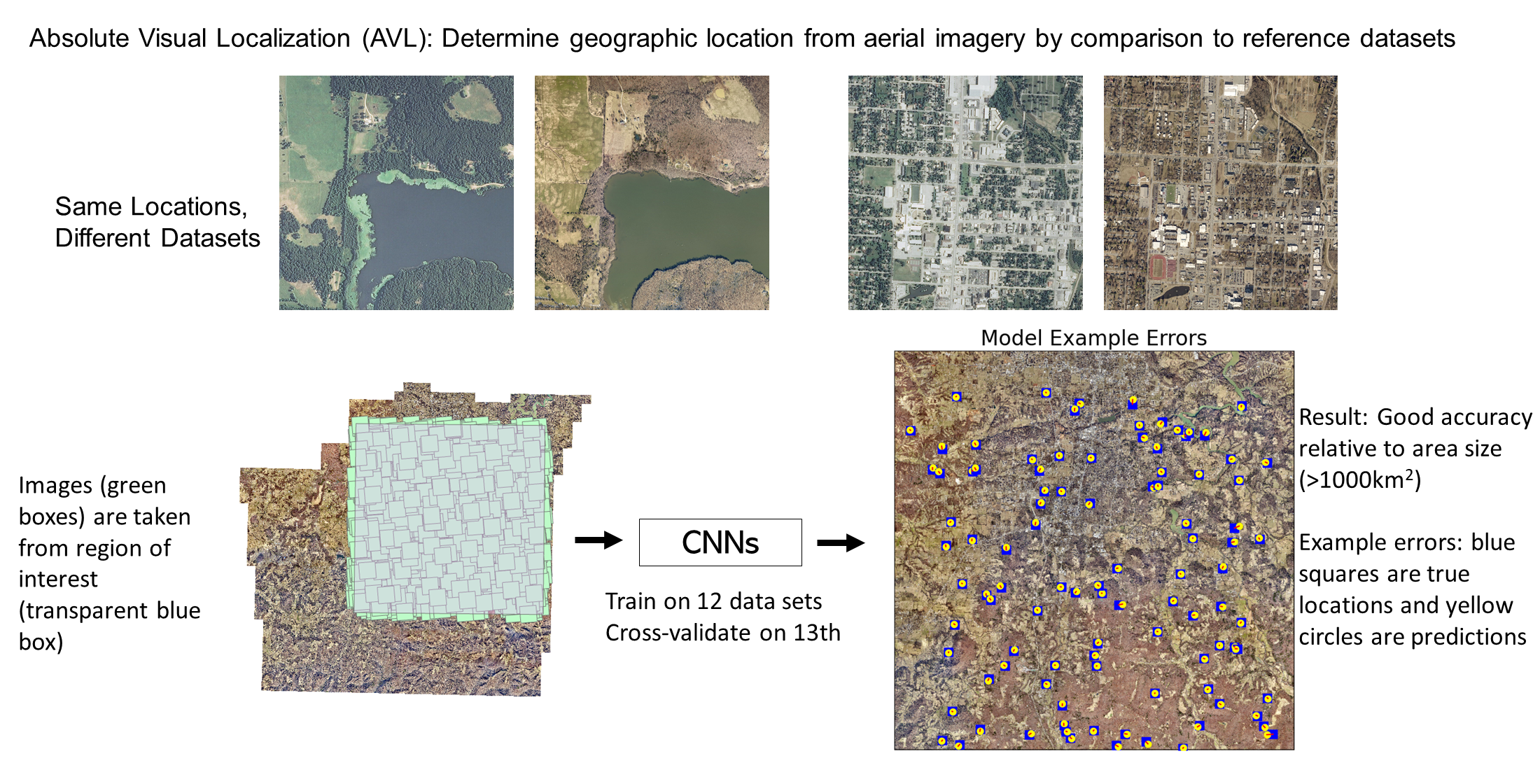
Figure 2.
Figure demonstrating cropping setup. The transparent square over the county represents the ROI. The green squares are individual 3km x 3km image chips extracted from the base data set. 2000 random chips are taken from each data set to ensure overcoverage, with different random chips for each data set. The final step before use in network training is a random crop from each chip, shown in red. Downsampling occurs at both the chipping and cropping stages. Chipping is an offline step performed once. Cropping is an online step performed during every epoch with different random crops.

Figure 3.
Figure demonstrating 100 sample errors of one of the runs (WaCo2020). Green is the true location, blue is the prediction, where predictions are connected to their true location by a red line. The background is of the holdout data set over the ROI.
Figure 3.
Figure demonstrating 100 sample errors of one of the runs (WaCo2020). Green is the true location, blue is the prediction, where predictions are connected to their true location by a red line. The background is of the holdout data set over the ROI.

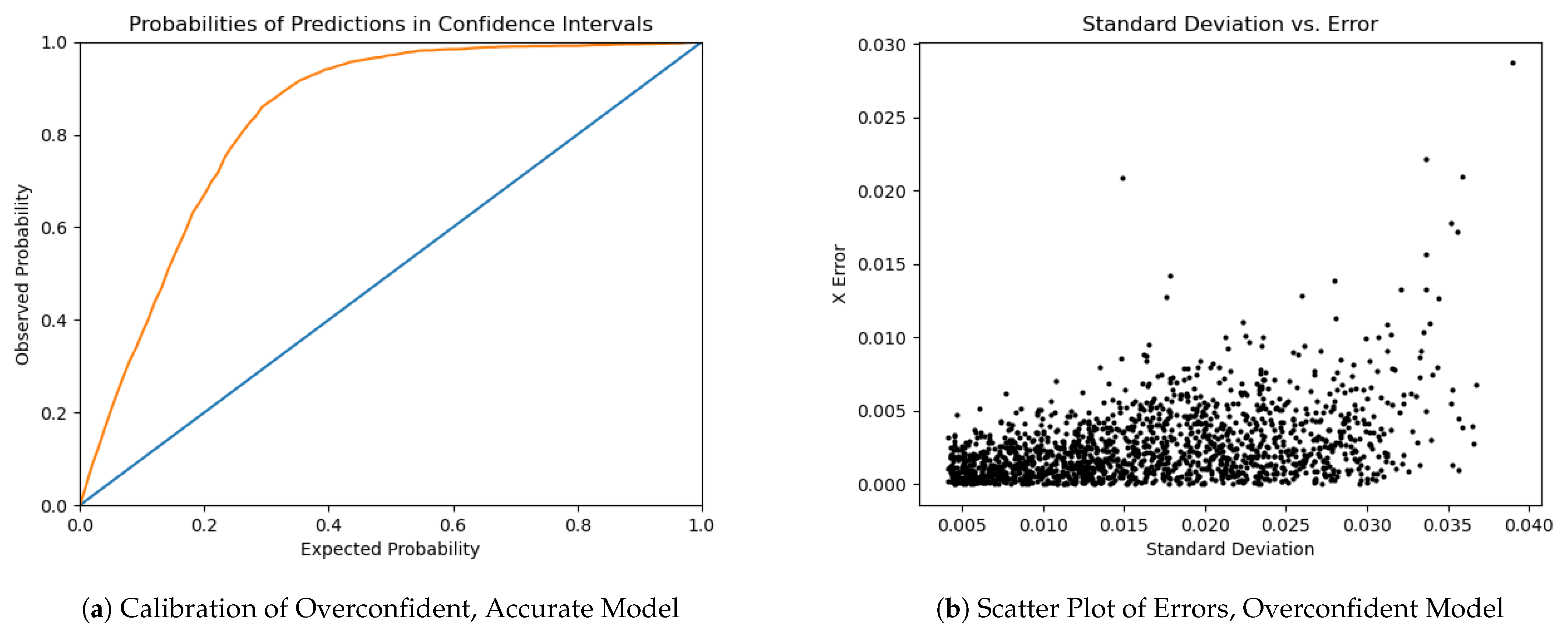
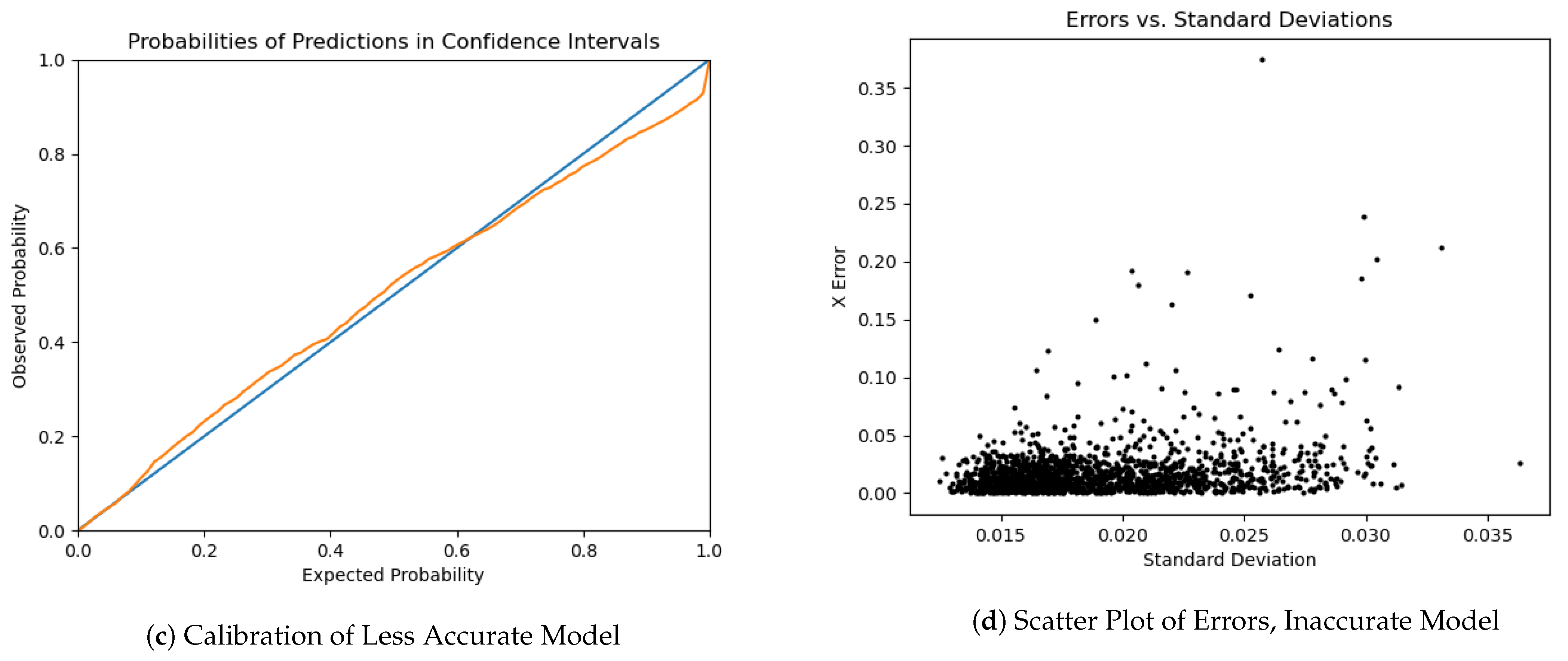
Figure 4.
Comparison of uncertainty calibration between an accurate model and a less accurate model. The units in (b,d) are normalized over the unit square ROI. The first model, shown in parts (a,b), had an average error of 149 m. It has poor uncertainty calibration; more of the true centers are contained in a given percent confidence interval than expected, meaning the model is underconfident. The second model, shown in (c,d), was incompletely trained, and only achieved an average error of 965 m. However, it showed better uncertainty calibration. Note, however, that some of the error sizes are unrealistically large given the standard errors, indicating the true uncertainty distribution is not Gaussian.


Table 1.
Model comparison for various built-in Keras models. Error is given as mean absolute error over the test set in normalized coordinates (NMAE). Note that performance should be about 0.25, the average distance to the center along either axis, if the model solely guesses (0.5, 0.5), the middle of the ROI, as an output. * EffNetB7 became overfitted extremely early in training. ** VGG16Conv was a custom modification of a smaller VGG-type architecture where pooling layers were replaced with strided convolution layers.
| Model | NMAE |
|---|---|
| EffNetB4 | 0.25 |
| EffNetB7 * | 0.25 |
| EffNetB0 | 0.18 |
| Resnet152V2 | 0.09 |
| VGG16 | 0.08 |
| VGG19 | 0.08 |
| VGG16Conv ** | 0.07 |
| Resnet152V2 | 0.07 |
| MobileNetv2 | 0.06 |
| Inception | 0.05 |
| Xception | 0.04 |
Table 2.
Field of view comparison. Absolute accuracy improved as field of view increased despite loss in visual resolution and confounding factors that favored smaller fields of view. Error is given as RMSE in normalized coordinates (NRMSE).
Table 2.
Field of view comparison. Absolute accuracy improved as field of view increased despite loss in visual resolution and confounding factors that favored smaller fields of view. Error is given as RMSE in normalized coordinates (NRMSE).
| Input Width/Height | NRMSE |
|---|---|
| 0.25 km | 0.3013 |
| 0.5 km | 0.2770 |
| 1 km | 0.0671 |
| 1.5 km | 0.0269 |
| 2 km | 0.0171 |
| 3 km | 0.0165 |
Table 3.
Loss function comparison. Holdout set was help constant as AO15. Error is the average distance error over the entire holdout set in normalized distances.
Table 3.
Loss function comparison. Holdout set was help constant as AO15. Error is the average distance error over the entire holdout set in normalized distances.
| Loss Function | Normalized Mean Euclidean Error |
|---|---|
| NegLogLikelihood | 0.0041 |
| MSE | 0.0198 |
| Euclidean Distance | 0.0232 |
Table 4.
Run replicability experiment results. Results are given in RMSE of the normalized error distances (NRMSE).
Table 4.
Run replicability experiment results. Results are given in RMSE of the normalized error distances (NRMSE).
| AO20 Run | NRMSE |
|---|---|
| 1 | 0.0556 |
| 2 | 0.0474 |
| 3 | 0.0481 |
| 4 | 0.0530 |
| 5 | 0.0541 |
Table 5.
Xception results on different holdout sets. Models were trained for 500 epochs. Error is reported in Euclidean distance.
Table 5.
Xception results on different holdout sets. Models were trained for 500 epochs. Error is reported in Euclidean distance.
| Test Set | Average Error | |
|---|---|---|
| Independent Normal | Bivariate Normal | |
| ADOP2006 | 188.2 m | 214.4 m |
| ADOP2017 | 172.7 m | 206.8 m |
| NAIP2006 | 189.2 m | 215.9 m |
| NAIP2009 | 323.8 m | 320.2 m |
| NAIP2010 | 146.4 m | 160.2 m |
| NAIP2013 | 129.9 m | 164.8 m |
| NAIP2015 | 173.4 m | 185.0 m |
| CAST2008 | 183.4 m | 251.3 m |
| AO15 | 124.3 m | 168.9 m |
| AO16 | 115.5 m | 156.5 m |
| AO17 | 127.6 m | 169.3 m |
| AO19 | 141.6 m | 174.1 m |
| AO20 | 148.7 m | 166.4 m |
Publisher’s Note: MDPI stays neutral with regard to jurisdictional claims in published maps and institutional affiliations. |
© 2021 by the authors. Licensee MDPI, Basel, Switzerland. This article is an open access article distributed under the terms and conditions of the Creative Commons Attribution (CC BY) license (https://creativecommons.org/licenses/by/4.0/).
Share and Cite
MDPI and ACS Style
Harvey, W.; Rainwater, C.; Cothren, J. Direct Aerial Visual Geolocalization Using Deep Neural Networks. Remote Sens. 2021, 13, 4017. https://0-doi-org.brum.beds.ac.uk/10.3390/rs13194017
AMA Style
Harvey W, Rainwater C, Cothren J. Direct Aerial Visual Geolocalization Using Deep Neural Networks. Remote Sensing. 2021; 13(19):4017. https://0-doi-org.brum.beds.ac.uk/10.3390/rs13194017
Chicago/Turabian StyleHarvey, Winthrop, Chase Rainwater, and Jackson Cothren. 2021. "Direct Aerial Visual Geolocalization Using Deep Neural Networks" Remote Sensing 13, no. 19: 4017. https://0-doi-org.brum.beds.ac.uk/10.3390/rs13194017
Note that from the first issue of 2016, this journal uses article numbers instead of page numbers. See further details here.