Article

Classification of Soybean Genotypes Assessed Under Different Water Availability and at Different Phenological Stages Using Leaf-Based Hyperspectral Reflectance

by
 Luis Guilherme Teixeira Crusiol
1,2,
Marcos Rafael Nanni
2,
Renato Herrig Furlanetto
2,
Rubson Natal Ribeiro Sibaldelli
3,
Everson Cezar
2,
Liang Sun
1,*,
José Salvador Simonetto Foloni
4,
Liliane Marcia Mertz-Henning
4,
Alexandre Lima Nepomuceno
4,
Norman Neumaier
4 and
José Renato Bouças Farias
4
1
Institute of Agricultural Resources and Regional Planning, Chinese Academy of Agricultural Sciences/Key Laboratory of Agricultural Remote Sensing, Ministry of Agriculture, Beijing 100081, China
2
Department of Agronomy, State University of Maringá, Maringá, PR 87020-900, Brazil
3
Londrina, Londrina, PR 86000-000, Brazil
4
Embrapa Soja (National Soybean Research Centre–Brazilian Agricultural Research Corporation), Londrina, PR 86001-970, Brazil
*
Author to whom correspondence should be addressed.
Submission received: 30 November 2020 / Revised: 29 December 2020 / Accepted: 3 January 2021 / Published: 6 January 2021
(This article belongs to the Special Issue Spectroscopic Analysis of Plants and Vegetation)

Abstract

:
Monitoring of soybean genotypes is important because of intellectual property over seed technology, better management over seed genetics, and more efficient strategies for its agricultural production process. This paper aims at spectrally classifying soybean genotypes submitted to diverse water availability levels at different phenological stages using leaf-based hyperspectral reflectance. Leaf reflectance spectra were collected using a hyperspectral proximal sensor. Two experiments were conducted as field trials: one experiment was at Embrapa Soja in the 2016/2017, 2017/2018, and 2018/2019 cropping seasons, where ten soybean genotypes were grown under four water conditions; and another experiment was in the experimental farm of Unoeste University in the 2018/2019 cropping season, where nine soybean genotypes were evaluated. The spectral data collected was divided into nine spectral datasets, comprising single and multiple cropping seasons (from 2016 to 2019), and two contrasting crop-growing environments. Principal component analysis, applied as an indicator of the explained variance of the reflectance spectra among genotypes within each spectral dataset, explained over 94% of the spectral variance in the first three principal components. Linear discriminant analysis, used to obtain a model of classification of each reflectance spectra of soybean leaves into each soybean genotype, achieved accuracy between 61% and 100% in the calibration procedure and between 50% and 100% in the validation procedure. Misclassification was observed only between genotypes from the same genetic background. The results demonstrated the great potential of the spectral classification of soybean genotypes at leaf-scale, regardless of the phenological stages or water status to which plants were submitted.

Graphical Abstract

1. Introduction

Soybean production plays a role in world crop production, with impacts on food security and financial markets. Brazil is responsible for one-third of the world’s soybean production [1,2]. Hence, precise, timely, and efficient understanding of soybean production is important for government and corporate decisions over technical issues, supply regulation, food security, financial market, and strategic planning relative to social environmental and economic policies [3,4,5,6].
Drought periods, as some of the most harmful factors that interfere in soybean production, especially when they occur in the reproductive phenological stages, have impaired around 30% of the Brazilian soybean production [7] and, in 38 years, caused financial losses of over 79 billion US$ [8]. Thus, exploring soybean genotypes with different mechanisms of drought tolerance has proven to be an essential and a necessary task to cope with water deficit periods [9,10].
In this context, accurate monitoring of soybean genotypes becomes extremely important due to the major international issue on intellectual property rights over seed technology [11,12,13,14,15,16,17]. The traditional methods for genotype identification in field conditions are laborious, time-consuming, and expensive. Hence, there is a rising need for methodologies to characterize soybean production in terms of location, extent, and genotype identification, which would facilitate royalty collection, better management of the seed genetics, and more efficient strategies over its production process.
Thus, remote sensing has great potential to provide information about soybean production areas in a less-time-consuming and non-destructive manner. Therefore, many scientists have been studying mapping soybean areas in the last years [18,19,20] and detecting plant diseases [21,22], invasive plants [23,24], nutritional deficiency [25,26,27,28], drought stress [29,30], characterizing crop phenological stages [31], and predicting grain yield [32,33,34].
The effectiveness of using leaf or canopy spectral response for genotype monitoring, identification, and classification has been demonstrated by several authors on different crop types. Aouidi et al. [35] applied mid-infrared spectral analysis from dried powdered leaf samples to discriminate five olive cultivars. Diago et al. [36] used hyperspectral imagery in laboratory to classify three grapevine varieties; Maimaitiyiming et al. [37] used canopy reflectance in field conditions to discriminate nine grapevine genotypes within two closely related species; while Gutiérrez et al. [38] used near-infrared leaf-based reflectance to classify grapevine varieties at site-specific and global modeling scales. Sinha et al. [39] differentiated twelve banana genotypes using leaf-based hyperspectral reflectance. Lin et al. [40] assessed the canopy hyperspectral response across the cropping season to monitor rice genotypes and developed their classification model at the booting stage. Ajayi et al. [41] evaluated the spectral behavior of twenty wheat genotypes with wide genetic background under irrigated and dryland conditions using hyperspectral data collected at the canopy level; while Garriga et al. [42] assessed the spectral response of 384 wheat genotypes at two phenological stages. Although much effort has been taken, there is a small number of research works addressed to discriminate and classify soybean genotypes by its spectral response [4,43,44,45] and data analysis from multiple phenological stages, cropping seasons, and water availability were not addressed.
One major issue regarding the spectral classification of soybean genotypes is the difficulty of evaluating soybean plants at the same phenological stage. In Brazil, the sowing time extends for more than a month within each region, which may impose some restrictions on the spectral classification of soybean genotypes in large areas because crops are never at the same phenological stage. Another issue is the occurrence of water deficits, which may undermine the spectral evaluation on a large scale since soybean plants are rarely under the same water status.
This research aims at spectrally classifying soybean genotypes, regardless of the phenological stage or water status to which plants are submitted, using leaf-based visible, near-infrared, and shortwave infrared hyperspectral reflectance. Our hypothesis is that soybean genotypes might present different spectral responses among them when assessed under different water availability and at different phenological stages, and our research question addresses the potential of leaf hyperspectral reflectance to distinguished and classify soybean genotypes assessed under different water availability and at different phenological stages.

2. Materials and Methods

2.1. Experimental Setup

Two experiments were conducted as field trials at two different locations (Figure 1): Londrina Municipality (as described in Section 2.1.1) and Presidente Bernardes Municipality (as described in Section 2.1.2), located in Parana State and Sao Paulo State, southern and southeast Brazil, respectively.

2.1.1. Experiment I: 2016/2017, 2017/2018, and 2018/2019 cropping seasons

This experiment (Figure 2) was undertaken in the experimental farm of the National Soybean Research Center (Embrapa Soja), a branch of the Brazilian Agricultural Research Corporation, located in Londrina Municipality, Paraná State, Southern Brazil (23°11′37′′ S, 51°11′03′′ W, 630 m above sea level), in the 2016/2017, 2017/2018, and 2018/2019 cropping seasons.
The climate of the study location is classified as Cfa according to the Köppen climate classification, i.e., subtropical climate, with mean temperature in the hottest month higher than 22 °C, with no defined dry season and rainfall concentrated in the summer months, which corresponds to the soybean cropping season [46,47]. Although dry season is not observed in the entire soybean crop season, periods of water deficit often provoke large yield losses [7].
The soil of the experimental area is characterized as Udox Oxisol [48], with the following characteristics: pH (in water): 4.9; H+Al: 3.5 cmolc dm−3; Al3+: 0.03 cmolc dm−3; Ca2+: 3.9 cmolc dm−3; Mg2+: 1.8 cmolc dm−3; K+: 0.7 cmolc dm−3; SB: 6.5; CTC: 10.0 cmolc dm−3; V%: 64.8; P: 24.2 mg dm−3; C: 15.6 g dm−3; 710 g kg−1 of clay; and 75 mm of water holding capacity (soil analysis in March 2016).
The following water condition treatments were distributed in the field plots: irrigated (IRR, receiving rainfall and irrigation when necessary, with a soil water matric potential between −0.03 and −0.05 MPa); non-irrigated (NIRR, receiving only rainfall); water deficit induced at the vegetative stages (DIV), and water deficit induced at reproductive stages (DIR). Soybean genotypes, with drought tolerance genes and different responses to water deficit, were distributed in the subplots. The collected data were analyzed following a split-plot model in a randomized complete block design, with four blocks.
To simulate water deficit, DIV and DIR plots were established under rainout shelters programmed to cover the subplots (at the vegetative or reproductive stages) when rainfalls above 0.1 mm were recorded. To prevent water lateral movement from outside into the soil, the plots had in their perimeter vertical concrete barriers (buried up to 90 cm depth). Once rainfalls had ceased, shelters automatically uncovered the plots. The DIV treatment was induced after plant establishment until the flowering period. From the flowering period to the harvesting period, the DIR treatment was induced in previously rain-watered plots. In turn, the DIV plots began to be rain watered.
In the 2017/2018 cropping season, there was no need for irrigation. Therefore, plants of IRR and NIRR treatments were under the same experimental conditions.
In the 2016/2017 cropping season, sowing was performed on 19 October 2016, the DIV treatment was induced from 25 November to 12 December 2016, and the DIR treatment was induced from 12 December 2016 until the harvesting period.
In the 2017/2018 cropping season, sowing was performed on 18 October 2017, the DIV treatment was induced from 20 November to 19 December 2017, and the DIR treatment was induced from 19 December 2017 until the harvesting period.
In the 2018/2019 cropping season, sowing was performed on 16 October 2018, the DIV treatment was induced from 26 November to 19 December 2018, and the DIR treatment was induced from 19 December 2018 to 14 January 2019 (when DIR plots began to receive rainfall again, until the harvesting period).
In 2016/2017 and 2017/2018 cropping seasons, five genotypes (‘1Ea15’, ‘2Ha11’, ‘2Ia4’, ‘BR16’, and ‘BRS 184’), named from now on, respectively, as genotypes 1, 2, 3, 4, and 5, were sown in the experimental plots mentioned above.
In the 2018/2019 cropping season, five different genotypes (‘1Ea2939’, ‘3Ma2’, ‘BRS 283’, ‘BRT18-0089’, and ‘BRT18-0201’), named from now on, respectively, as genotypes 6, 7, 8, 9, and 10, were sowed in those plots and genotypes 1, 2, 3, 4, and 5 were sowed in secondary experimental plots and subjected to the NIRR treatment, receiving only rainfall.
The spectral assessments performed in 2016/2017, 2017/2018, and 2018/2019 cropping seasons are described in Section 2.3 (Spectral data acquisition and processing).

2.1.2. Experiment II: Unoeste University Experiment

This experiment (Figure 3) was conducted in the experimental farm of the Unoeste University, located in Presidente Bernardes Municipality, São Paulo State, Southeast Brazil (22° 17′ 08” S, 51° 40′ 27” W), in the 2018/2019 cropping season.
The study area, which soil and climatic characteristics are distinct from Londrina-PR, indicating differences between their crop-growing environments [49], is located on a climate transition between Cfa and Aw (i.e., tropical climate, with mean temperature in the coolest month higher than 18 °C, with rainfall concentrated in the summer months, and less than 60 mm of rainfall in the driest month), according to the Köppen climate classification [47].
The soil of the experimental area is characterized as Udult Ultisol [48] with the following characteristics: pH (in water): 5.6; H+Al: 1.76 cmolc dm−3; Al3+: 0.0 cmolc dm−3; Ca2+: 2.95 cmolc dm−3; Mg2+: 1.6 cmolc dm−3; K+: 0.17 cmolc dm−3; SB: 4.7; CTC: 6.5 cmolc dm−3; V%: 72.8; P: 6.7 mg dm−3; C: 14.2 g dm−3; 170 g kg−1 of clay; and 55 mm of water holding capacity (soil analysis in April 2018).
Following the soybean production technologies [50], soybean genotypes 1, 2, 3, 4, 5, 6, 8, 9, and 10 were sowed in experimental plots subjected to the non-irrigated treatment, receiving only rainfall. The sowing date was 18 October 2018.
The spectral assessments performed in the Unoeste University experiment are described in Section 2.3 (Spectral data acquisition and processing).

2.2. Weather Monitoring

Weather data—air temperature, relative air humidity and rainfall—were monitored by the weather station located within the experimental areas, as described by Sibaldelli and Farias [51,52,53] and the climatic water balance was calculated according to Thornthwaite and Mather [54] for each experimental treatment of each cropping season. The calculated climate water balances are presented in Figure 4.
It is possible to observe, by the deficits of the climate water balances, the efficiency of the induced water deficit in the DIV at December 1 and 2 10-day periods (Figure 4a,e,i) and DIR treatments at December 3 and January 1, 2, and 3 10-day periods (Figure 4b,f,j) in the three cropping seasons.
The water deficit imposed on the DIR treatment was demonstrated to be more harmful than the water deficit imposed on DIV plants, because of the longer period to which plants were deprived of natural rainfall. Besides that, the water deficit in the DIR occurred during the reproductive stages of plant development, when plants are more sensitive to the water deficit since the reproductive structures and grains are being formed. During this period, the plant reaches its maximum need for water, close to 8 mm per day.
Although severe natural water deficit was not observed in the 2016/2017 cropping season (Figure 4c), the irrigation was enough to maintain plants under good conditions of water availability on November 3 and December 1 10-day periods (Figure 4d).
Severe natural water deficit was observed in the 2018/2019 cropping season (Figure 4k), both in vegetative (Figure 4i) and reproductive (Figure 4j) periods and the irrigated treatment promoted good conditions of water availability at December 1, 2, and 3, January 2, and February 2 10-day periods (Figure 4l).
The climate differences between Embrapa Soja and Unoeste University are demonstrated by the water balance of the non-irrigated treatment of both experimental areas (Figure 4h,k).

2.3. Spectral Data Acquisition and Processing

Soybean leaf reflectance was collected by the FieldSpec 3 Jr spectroradiometer (Analytical Spectral Devices, Boulder, CO, USA), with a spectral resolution of 3 nm between 350 and 1400 nm and 30 nm between 1400 and 2500 nm (Figure 5).
Each spectral reading was the average of 20 internal automatic spectral readings, and the output spectra were given in single bands of 1 nm intervals, 2151 spectral bands. To prevent illumination interferences of adjacent targets and atmospheric scattering and attenuation, we used the leaf reflectance plant probe device connected to the FieldSpec by a one-meter optical bare fiber (Figure 5c). The plant probe device has an internal 99% reflectance board (Spectralon®), used as reflectance standard, and a 1% reflectance opaque and black board, used during the spectral assessment to ensure pure leaf reflectance spectra collection, without the need for applying spectral filters for noise remove and data smooth [4,55,56,57].
The central leaflet of the fullest expanded third trifoliate leaf from the top was selected for spectral acquisition. A total of 9061 leaf reflectance samples were collected and divided into nine spectral datasets (Table 1), as described below.
1)
Embrapa 2016/2017 was comprised of spectral data of genotypes 1, 2, 3, and 4 collected in 29, 34, 45, 58, 70, 90, and 113 days after sowing (DAS) in the four experimental treatments during the 2016/2017 cropping season at Embrapa Soja, with four subsamples in each plot, resulting in 1776 leaf reflectance spectra, totaling 444 spectral samples.
2)
Embrapa 2017/2018 was comprised of the spectral data of genotypes 1, 2, 3, 4, and 5 collected in 30, 38, 43, 58, 79, 97, 107, and 113 DAS in the four experimental treatments during the 2017/2018 cropping season at Embrapa Soja, with four subsamples in each plot, resulting in 1920 leaf reflectance spectra, generating 640 spectral samples.
3)
Embrapa 2018/2019 [I] was comprised of spectral data of genotypes 1, 2, 3, 4, and 5 collected in 42, 51, 58, 65, 80, 88, 95, 102, and 108 DAS in the ‘non-irrigated’ treatment during the 2018/2019 cropping season at Embrapa Soja, totaling 900 spectral samples.
4)
Embrapa 2018/2019 [II] was comprised of spectral data of genotypes 6, 7, 8, 9, and 10 collected in 42, 51, 58, 65, 80, 88, 95, 102, and 108 DAS in the four experimental treatments during the 2018/2019 cropping season at Embrapa Soja, with four subsamples in each plot, resulting in 2880 leaf reflectance spectra and 720 spectral samples.
5)
Embrapa 2016–2019 was comprised of the ‘Embrapa 2016/2017’, ‘Embrapa 2017/2018’, and ‘Embrapa 2018/2019 [I]’ spectral datasets, adding up to 1984 spectral samples of genotypes 1, 2, 3, 4, and 5.
6)
Unoeste 2018/2019 [I] was comprised of spectral data of genotypes 1, 2, 3, 4, and 5 collected in 51, 62, 92, and 107 DAS during the 2018/2019 cropping season at the Unoeste University farm, resulting in 525 spectral samples.
7)
Unoeste 2018/2019 [II] was comprised of spectral data of genotypes 6, 8, 9, and 10 collected at 51, 62, 92, and 107 DAS during the 2018/2019 cropping season at the Unoeste University farm, totaling 420 spectral samples.
8)
Embrapa 2016–2019 + Unoeste [I] was comprised of the ‘Embrapa 2016–2019’ and ‘Unoeste 2018/2019 [I]’ spectral datasets, for a total of 2509 spectral samples of genotypes 1, 2, 3, 4, and 5.
9)
Embrapa 2018/2019 + Unoeste [II] was comprised of the ‘Embrapa 2018/2019 [II]’ and ‘Unoeste 2018/2019 [II]’ spectral datasets, summing up to 1140 spectral samples of genotypes 6, 7, 8, 9, and 10.
The statistical analysis of each spectral dataset composed by field assessments was performed, aiming at the classification of soybean genotypes by their spectral responses, comprising different phenological stages and water status to which plants were submitted. Wavelengths between 350 and 399 nm were not considered for spectral analysis because of the frequent noises observed on vegetation analysis in this spectral interval [58,59].

2.4. Statistical Analysis

2.4.1. Principal Component Analysis (PCA)

The principal component analysis (p-value <0.05) was performed by Unscrambler X software, version 10.4 (Camo Analytics), as an indicator of whether the variance of the reflectance spectra among genotypes within each spectral dataset could be explained, and how effectively soybean genotypes could be clustered.
PCA, a widely used data mining method that reduces the number of variables to be analyzed (e.g., spectral bands), promotes, by a covariance matrix composed by all spectral bands of the full reflectance spectra, the transformation of those variables into a new group of variables, called principal components (PCs). The PC can be described as the linear combination of all analyzed variables to explain their variance, and each PC has its associated score, which denotes the percentage of variance that can be explained. The first principal component (PC1) carries the most information of data variance, the second principal component carries the residual information of PC1, the third principal component carries the residual information of PC2 and so on [60,61]. According to Wang [62], when the cumulative contribution of the first several components is more than 80%, the remaining components can be omitted in further analysis.

2.4.2. Linear Discriminant Analysis (LDA)

Linear discriminant analysis (LDA), performed by the Statistical Analysis System® software (SAS Institute, Inc., Cary, NC, USA), was used to obtain a model of classification of each reflectance spectra of soybean leaves into each soybean genotype. Before the LDA, the stepwise procedure was carried out to select the wavelengths that statistically distinguish the analyzed soybean genotypes and to maximize the Mahalanobis distance among the soybean genotypes [44]. In this procedure, each variable (wavelength) is added (forward) and removed (backward) from a multilinear regression function, evaluated by the F-test and by the Wilk’s Lambda value, following the likelihood principle [27,63,64,65,66,67]. Variables with p-value <0.05 (defined a priori) were added and not removed in/from the function. The stepwise procedure was carried out until no variable could be entered or removed from the function [27,67,68]. Using the selected wavelengths, the linear discriminant analysis was carried out.
Each spectral dataset (Table 1) was randomly divided by the SAS software into two subsets: calibration and validation, containing 60% and 40% of the reflectance spectra, respectively. The LDA was carried out using the calibration subset, of which accuracy was evaluated by the replacement of each reflectance spectra (60%) in the generated linear discriminant function and the percentage of success in their classification into the correct soybean genotype. The validation subset (40%) was tested in the linear discriminant function (generated using the calibration subset) and the validation accuracy was evaluated by the replacement of each reflectance spectra (40%) in the linear discriminant function (60%) and the percentage of success in their classification into the correct soybean genotype. The LDA was repeated 50 times in the calibration and validation process to avoid a tendency in the discriminant function [69].
The results of the LDA of each spectral dataset is provided as a contingency matrix, expressed in percentages of correct classification and misclassification among all evaluated groups (soybean genotypes). The contingency matrix was transformed into graphic bars for better visual interpretation.

3. Results and Discussion

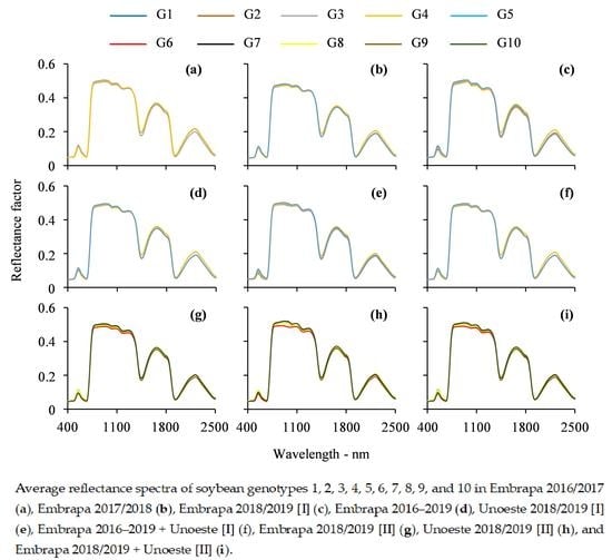
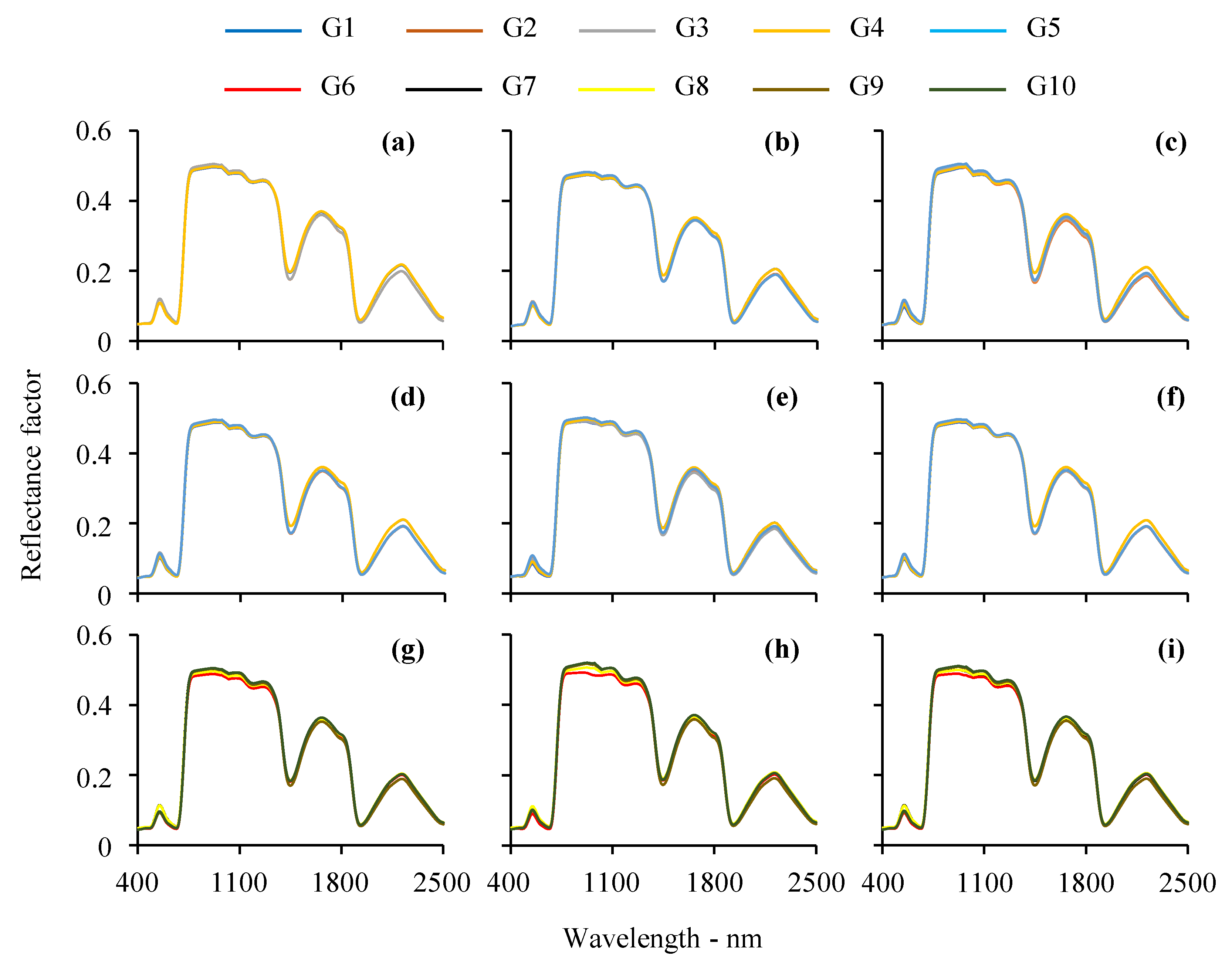
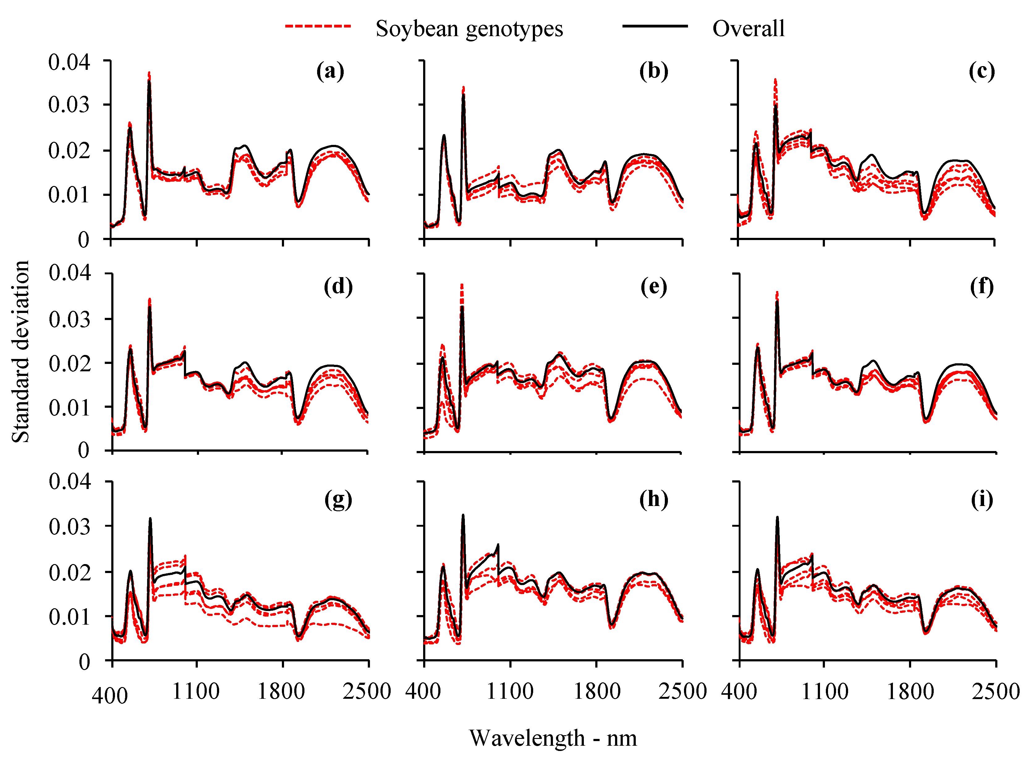
3.1. Visual Analysis of Leaf Reflectance Spectra

Figure 6 displays the average reflectance spectra of each soybean genotype in each spectral dataset (defined in Table 1), in which a very small difference among the average reflectance spectra can be observed, and the shape of the spectral curve does not vary among genotypes and spectral datasets.
In the spectral datasets composed by genotypes 1, 2, 3, 4, and 5 (Figure 6a–f), a close relation between genotypes 1 and 4 and among genotypes 2, 3, and 5 was observed around 1400 and 2220 nm. Similarly, in the spectral datasets composed by genotypes 6, 7, 8, 9, and 10 (Figure 6g–i) differences can also be observed around 1400 and 2200 nm, indicating three groups of genotypes. Such differences are due to the interaction between crop phenological stage, plant water status, and environmental conditions. However, the spectral variability among vegetation groups is not the same across the wavelengths due to leaf biochemical properties and structure [37,66,67,68,69].
Figure 7 presents the standard deviation of soybean genotypes and the overall standard deviation of each spectral dataset (defined in Table 1). The standard deviation, comprising multiple days of assessment, different levels of water availability, and distinct crop-growing environments, was lower than 0.04 in all spectral datasets. The lowest standard deviation was observed in wavelengths corresponding to the blue and red spectrum, around 450 and 670 nm. In wavelengths corresponding to the green spectrum, the standard deviation presented a peak.
Price [70], Breunig et al. [71], and Crusiol [72] have discussed the influence of crop development in the spectral reflectance. Specifically, in the visible (VIS) wavelengths (between 400 and 720 nm), associated with the photosynthetic active radiation [67,73,74,75,76,77], changes in plant phenological development result in changes in light absorption. Therefore, since plants were evaluated on different dates across cropping season, differences were expected in their reflectance at visible wavelengths. It is worth mentioning that the highest peak of standard deviation among all wavelengths was observed around 710 nm in all spectral datasets, close to the slope between red and near-infrared wavelengths.
A complete review of the interference of plant water status in crop spectra was written by Damm et al. [78], emphasizing that plants under water deficit demonstrate reflectance values higher than plants submitted to good conditions of water availability. Although the entire spectrum between 400 and 2500 nm might be affected by vegetation water status, the shortwave infrared is the one that shows the most conspicuous changes in reflectance due to changes in plant water status.
In the near-infrared (NIR, between 720 and 1300 nm), the interaction of the incident light inside the mesophyll, leading to internal scattering, can be affected by the water content [67,79,80,81]. Hence, at higher levels of water content, higher light absorption is observed, leading to lower reflectance values.
In shortwave infrared spectrum (SWIR, between 1300 and 2500 nm), spectral interval most associated to the vegetation water status [82,83,84], the standard deviation showed to be around 0.02 in both spectral datasets. Although wavelengths around 1900 nm are influenced by the leaf water content [85], the lowest standard deviation across the SWIR spectrum was observed on these wavelengths, demonstrating low variability within all datasets.

3.2. Principal Component Analysis—PCA

Figure 8 displays the results of the PCA of each spectral dataset (defined in Table 1). In each bar (spectral dataset), the first, second, and third principal components represent the percentage of the variance that can be explained (score). Among the evaluated datasets, none of them presented explained variances (score) in the first PC lower than 47% and all of them presented cumulative scores in the first and second PCs over 80%. The cumulative scores in the three first PCs of all spectral datasets showed to be over 94%. Those results indicate the possibility of discrimination of soybean genotypes within each spectral dataset.
The obtained results are in agreement with previous research findings addressing the use of PCA to demonstrate spectral differences in vegetation analysis, when the two or three first PCs explained more than 90% of the spectral variance [86,87,88,89,90]. Analyzing soybean leaf spectra of four genotypes at a single day assessment, Silva Junior et al. [4] obtained cumulative scores in the first and second PCs over 95%.
The loading correlation of each PCA, expressed in (r), was also evaluated. Defined as the correlation of each variable (wavelength) with the principal component, the loadings describe the importance of each wavelength to the PC [61,91]. This procedure was also adopted by Thenkabail et al. [64], Foster et al. [86], Guzmán et al. [87], and Lebow et al. [92]. In all spectral datasets, the first principal component was mainly influenced by SWIR wavelengths and by NIR wavelengths with lower importance. The second principal component of the spectral datasets was mainly influenced by NIR wavelengths, but also have, with lower importance, the influence of SWIR wavelengths. Only in the third principal component, VIS wavelengths were found to have loadings with (r) > 0.7. Thenkabail et al. [64], Foster et al. [86], and Clark et al. [93] also described the SWIR wavelengths to be more suitable to distinguish vegetation spectra.

3.3. Stepwise Procedure

The spectral wavelengths selected in the stepwise procedure of each spectral dataset (defined in Table 1) are represented in Figure 9.
It is possible to observe that many wavelengths are significant (p < 0.05) to differentiate the soybean genotypes within each spectral dataset. The lowest number of selected wavelengths, 16, was obtained for the ‘Embrapa 2016/2017’ spectral dataset and the maximum for the ‘Embrapa 2018/2019 + Unoeste [II]’ spectral dataset, 138. The numbers of selected wavelengths in each spectral dataset were: 75 (Embrapa 2017/2018), 96 (Embrapa 2018/2019 [I]), 118 (Embrapa 2016–2019), 81 (Unoeste 2018/2019 [I]), 127 (Embrapa 2016–2019 + Unoeste [I]), 99 (Embrapa 2018/2019 [II]), and 117 (Unoeste 2018/2019 [II]).
Compared to several research works aiming at discriminating reflectance spectra, our work studied a larger number of selected wavelengths. Some authors selected less than 10 spectral wavelengths [86,90,94], while others selected from 10 to around 25 spectral wavelengths [44,95,96,97,98]. A review of selected spectral bands for species classification can be seen in Fassnacht et al. [99].
Wavelengths selected in the stepwise procedure were well distributed in the spectral interval from 400 to 2500 nm, except for one dataset (Embrapa 2016/2017). However, it is important to emphasize the spectral gap in selected wavelengths between 700 and 1000 nm in most spectral datasets, comprising the red-edge and near-infrared spectrum. Major attention is required in those wavelengths, highlighting possible biotic and abiotic factors that may interfere in the spectral response and differentiation of genotypes [67].

3.4. Linear Discriminant Analysis–LDA

Figure 10 presents the results of the linear discriminant analysis of the Embrapa 2016/2017 (a), Embrapa 2017/2018 (b), and Embrapa 2018/2019 [I] (c) spectral datasets.
In the 2016/2017 cropping season (Figure 10a), the calibration procedure demonstrated accuracy between 61 and 67% for all genotypes. Since the validation procedure was performed using external samples, it was expected to have lower accuracy compared to the calibration procedure. Therefore, the validation procedure revealed an accuracy between 50 to 61% for all genotypes.
Figure 10b shows that in the 2017/2018 cropping season the calibration procedure had an accuracy between 79 and 87%, while the validation procedure presented accuracy from 52 to 66% for all genotypes. Higher accuracy of the calibration procedure, which was expected, was also found in the 2018/2019 cropping season (Figure 10c) when the obtained accuracy was between 90 and 92% in the calibration procedure, and between 73 and 82% in the validation procedure for all genotypes.
There was an association between genotypes 1 and 4 (red and blue bars) and between genotypes 2 and 3 (grey and yellow bars) (Figure 10a). In the 2017/2018 and 2018/2019 cropping seasons, genotypes 2 and 3 were also associated with genotype 5 (green bars) (Figure 10b,c).
Therefore, in the 2016/2017 cropping season, in the calibration procedure, genotype 1 had 28% of their spectra classified as genotype 4, and genotype 4 had 33% of their spectra classified as genotype 1. In the same context, genotype 2 had 31% of their spectra classified as genotype 3, and genotype 3 had 35% of their spectra classified as genotype 2. This association could be consistently observed in the three cropping seasons in the calibration and validation procedures.
In the 2017/2018 cropping season (Figure 10b), in the calibration procedure, genotype 2 had 11% of their spectra classified as genotype 3 and 9% classified as genotype 5. Genotype 3 had 10% of their spectra classified as genotype 2 and 11% classified as genotype 5, and genotype 5 had 8% of their spectra classified as genotype 2 and 11% classified as genotype 3.
Their genetic background explains the close relations between the genotypes 1 and 4, and among genotypes 2, 3, and 5. In the process of genetically transforming soybean with drought tolerance genes, genotype 1 was developed from genotype 4, and genotypes 2 and 3 were developed from genotype 5. Therefore, it was expected that genotypes (isolines) carrying the same genetic background of the parental genotypes, showing very similar characteristics, would result in spectral misclassification among them.
From the 2016/2017 to 2018/2019 cropping seasons, an increase in the accuracy of classifying the five soybean genotypes was observed. Such accuracy enhancement may be due to the insertion of one extra genotype (G5), from the 2016/2017 to 2017/2018 cropping season, and the higher number of spectral samples (Table 1).
Furthermore, in the 2017/2018 cropping season, spectral assessments were better distributed across the phenological stages, comprising three assessments (97, 107, and 113 DAS) in R5 stage [100], while in the 2016/2017 cropping season only two assessments (90 and 113 DAS) were performed in the R5 stage. Galvão et al. [44] and Silva Junior et al. [4] performed their soybean discrimination in the R5 phenological stage, but they did not compare different phenological stages.
Moreover, in the 2017/2018 cropping season, irrigation was not performed, which may have reduced the spectral variability within genotypes since plants under IRR and NIRR treatments were under the same water condition. The interference of water deficit in the spectral response of vegetation has been well determined by many authors [82,83,84,85].
The accuracy enhancement observed in the 2018/2019 cropping season occurred by three reasons: higher number of collected spectra per genotype (Table 1); better distribution in time of spectral assessments across the phenological stages relative to the previous cropping seasons; and because soybean plants were subjected only to the non-irrigated treatment, which reduced the spectral variance among experimental treatments.
Figure 11 displays the results of the linear discriminant analysis of the Embrapa 2016–2019 (a), Unoeste 2018/2019 [I] (b), and Embrapa 2016–2019 + Unoeste 2018/2019 [I] (c) spectral datasets.
In general, the linear discriminant analysis of the ‘Embrapa 2016–2019’ spectral dataset (performed using 1984 reflectance spectra of five soybean genotypes under variant water status and phenological stages, assessed at 24 dates, in three cropping seasons) represented an average accuracy of those cropping seasons (Figure 11a).
Therefore, the accuracy in calibration and validation subset of the LDA ranged, among soybean genotypes, from 70 to 81%, and from 58 to 71%, respectively. As discussed in each of the three cropping seasons, the close spectral relation between genotypes 1 and 4 and among genotypes 2, 3, and 5 was sustained.
Although the results achieved for the ‘Embrapa 2016–2019’ spectral dataset seemed to represent an average accuracy of three cropping seasons, it strengthens the possibility of continuous development, year by year, of the linear discriminant function on every single cropping season, which could comprise spectral information about soybean plants under different environmental conditions during the growing period.
The best results in the LDA of genotypes 1, 2, 3, 4, and 5 were obtained in the ‘Unoeste 2018/2019 [I]’ spectral dataset (Figure 11b). In the calibration procedure, the accuracy was close to the maximum, 98% for genotypes 2, 3, and 5, and 100% for genotypes 1 and 4. Good results were also obtained in the validation procedure, with accuracy ranging from 86 to 98%.
Since soybean crops are widely spread over the Brazilian territory, Embrapa Soja has grouped soybean production areas in five macro- and twenty micro-regions based on their soil and climatic characteristics to match specific maturity groups of soybean genotypes. This grouping allows for better recommendations of technical practices for soybean production [48]. Therefore, Londrina—PR and Presidente Bernardes—SP are located in distinct macro-regions, indicating differences between their crop-growing environments.
Compared to Embrapa, enhancements in the accuracy of the LDA in the ‘Unoeste 2018/2019 [I]’ spectral dataset may be related to the crop-growing environment of Unoeste University, which is more prone to drought stress, characterized by soil with lower water holding capacity, higher air temperatures, and lower rainfall. Thus, the expression of drought tolerance genes in the soybean genotypes at Unoeste University could be higher, highlighting physiological differences among soybean genotypes [9,10,101,102,103], promoting spectral differences.
Analyzing all spectral datasets containing reflectance spectra of genotypes 1, 2, 3, 4, and 5, collected in two contrasting crop-growing environments (Embrapa 2016–2019 + Unoeste 2018/2019 [I] spectral dataset) (Figure 11c), a decrease in the accuracy relative to the ‘Embrapa 2016–2019’ and ‘Unoeste 2018/2019 [I]’ spectral datasets was observed. The achieved accuracy in the calibration procedure ranged, for all genotypes, from 68 to 79% and in the validation procedure from 53 to 69%.
However, the ‘Embrapa 2016–2019 + Unoeste 2018/2019 [I]’ spectral dataset comprises 2509 reflectance spectra, collected in three cropping seasons, under four different levels of water availability, at 28 days of spectral assessment and at two locations with contrasting crop-growing environments. Therefore, regardless of the phenological stages or water status to which plants were submitted, the linear discriminant function could classify soybean genotypes with over 53% of accuracy and almost all misclassification was observed between genotypes from the same genetic background. Hence, the LDA of the ‘Embrapa 2016–2019 + Unoeste 2018/2019 [I]’ spectral dataset classified the 2509 leaf reflectance spectra into the correct group of genetic background (genotype 1 and 4; and genotypes 2, 3, and 5) with accuracy over 97% (red and blue bars summed and analyzed together; and grey, yellow, and green bars summed and analyzed together), both in the calibration and validation procedures.
To reinforce the obtained results in LDA, five different genotypes (genotype 6, 7, 8, 9, and 10) were evaluated both at Embrapa and Unoeste field experiments. Figure 12 displays the results of the linear discriminant analysis (calibration and validation subsets) of the ‘Embrapa 2018/2019 [II]’ (a), ‘Unoeste 2018/2019 [II]’ (b), and ‘Embrapa 2018/2019 [II] + Unoeste 2018/2019 [II]’ (c) spectral datasets.
In the ‘Embrapa 2018/2019 [II]’ spectral dataset (Figure 12a), in the calibration procedure, the accuracy in the classification of soybean genotypes 6, 7, 8, 9, and 10 ranged from 89% to 100%, while in the validation procedure the accuracy showed to be between 74% and 100%. It is possible to observe a close spectral relation between genotypes 7 and 8 in the calibration and validation procedure, and between genotypes 9 and 10 in the validation procedure. In soybean genetic improvement, genotype 7 was developed from genotype 8, and genotypes 9 and 10 have the same genetic background. Hence, as discussed in the previous spectral datasets, misclassification among genotypes from the same genetic background was expected.
Figure 12b presents the results of the LDA of the ‘Unoeste 2018/2019 [II]’ spectral dataset. The accuracy of LDA in the calibration procedure was 100% for all genotypes. In the validation procedure, genotypes 6 and 8 had 100% of their spectra correctly classified, while genotypes 9 and 10 had little misclassification between them, with 99% and 98% accuracy, respectively. The fact that genotype 8 achieved 100% accuracy may be due to the absence of genotype 7 in this experiment, avoiding the spectral misclassification between them.
As previously reported, the linear discriminant analysis performed using spectral data collected in Unoeste University, a crop-growing environment more prone to drought, presented higher accuracy than the LDA using spectral data collected at Embrapa. This higher accuracy can be due to genotype differential gene expression under drought conditions. Besides that, plants were subjected only to the non-irrigated water condition, decreasing the spectral variability.
The results of the LDA of the ‘Embrapa 2018/2019 [II] + Unoeste 2018/2019 [II]’ spectral dataset is displayed in Figure 12c. The accuracy in the calibration procedure ranged from 82% to 100% and in the validation procedure from 75% to 100%.
It was observed an accuracy decrease in the classification of soybean genotypes compared to the LDA performed using spectral data from Embrapa (Figure 12a) and Unoeste University (Figure 12b). These results corroborate the results found in the LDA of the ‘Embrapa 2016–2019 + Unoeste 2018/2019 [I]’ spectral dataset (Figure 11c), when spectral data collected in contrasting crop-growing environment (Embrapa and Unoeste University), led to a decrease in the accuracy of the LDA.
The linear discriminant analysis performed using genotypes 6, 7, 8, 9, and 10 achieved accuracy over 66% in the classification of soybean genotypes, regardless of the phenological stages or water status to which plants were submitted (Figure 12a–c), and misclassification was only observed between genotypes from the same genetic background.
Considering the three groups of genetic background (genotype 6; genotypes 7 and 8; and genotypes 9 and 10), the LDA classified all the 1140 leaf reflectance spectra into the correct group with an accuracy of 100% (red bars; yellow and grey bars summed and analyzed together; blue and green bars summed and analyzed together) both in the calibration and validation procedures.
Although few papers have been aimed at classifying soybean genotypes by their spectral response, the accuracy achieved in this paper was high when compared to other papers. Breunig et al. [43] stated that the accuracy may be influenced by the classification method used, ranging from 44% to 100%. However, those authors performed the pixel classification of just five soybean genotypes using only a single Hyperion scene, in a single day, precluding the application of the obtained results to long-term analyses.
In the same context, Galvão et al. [44] achieved over 89% of accuracy in the classification of three soybean genotypes using Hyperion scenes. Although those authors evaluated two cropping seasons, one scene at each, they did not analyze the two cropping seasons together, which compromises the continuous development of spectral classification models through different cropping seasons. Silva Junior et al. [4] achieved over 97% of accuracy in the spectral classification of four soybean genotypes. However, like the previously mentioned authors, they evaluated soybean plants in only one date.
Nevertheless, it should be reinforced that the spectral datasets analyzed in this paper were composed by leaf reflectance spectra acquired under variant conditions of water availability, in three cropping seasons and at different phenological stages in two contrasting crop-growing environments, demonstrating the possibility of linear discriminant functions to be applied in large areas of soybean crops.

4. Conclusions

This paper evaluated the potential of the spectral classification of soybean genotypes using hyperspectral sensor and linear discriminant analysis. A very small difference among the average reflectance spectra of soybean genotypes could be observed, and the shape of the spectral curve did not vary among genotypes.
In each dataset, the principal component analysis explained over 94% of the spectral variance of soybean genotypes in the first three PCs, with higher importance of SWIR wavelengths. The stepwise procedure selected from 16 to 138 spectral bands capable to distinguish soybean genotypes.
The linear discriminant analysis, using leaf reflectance of soybean genotypes under variant water status and at different phenological stages, achieved accuracy between 61% and 100% in the calibration procedure and between 50% and 100% in the validation procedure. Misclassification was observed between genotypes from the same genetic background. Thus, if summed and analyzed together, soybean genotypes from the same genetic background could achieve accuracy over 93%, both in calibration and validation procedure.
The obtained results demonstrate the great potential of the spectral classification of soybean genotypes at leaf-scale regardless of the phenological stages or water status to which plants were submitted.

Author Contributions

Conceptualization: L.G.T.C., M.R.N., R.H.F. and R.N.R.S. Methodology: L.G.T.C., R.H.F., M.R.N., R.N.R.S., J.S.S.F., L.M.M.-H., A.L.N., N.N. and J.R.B.F. Software, L.G.T.C., R.H.F. and E.C. Formal analysis: L.G.T.C., M.R.N., R.N.R.S., N.N. and J.R.B.F. Data curation: L.G.T.C., M.R.N. and J.R.B.F. Writing—original draft preparation: L.G.T.C. Visualization: M.R.N., J.R.B.F. and L.S. Project administration: M.R.N., J.R.B.F. and L.S. Funding acquisition: M.R.N., J.R.B.F. and L.S. All authors have read and agreed to the published version of the manuscript.

Funding

This work has been funded by the National Council for Scientific and Technological Development–CNPq; Central Public-Interest Scientific Institution Basal Research Fund [Y2020GH14] and the Talented Young Scientist Program—China Science and Technology Exchange Center [Brazil–19-004].

Data Availability Statement

The data that support the findings of this study are available from the author L.G.T.C.

Conflicts of Interest

The authors declare no conflict of interest.

References

  1. CONAB (National Company of Food Supply). Brazilian Crop Assessment–Grain, 2019/2020 Crops, Sixth Inventory Survey, March/2020. 2020. Available online: https://www.conab.gov.br/info-agro/safras/graos/boletim-da-safra-de-graos (accessed on 25 March 2020).
  2. USDA (United States Department of Agriculture). World Agricultural Production. Circular Series WAP 3-20, March 2020. 2020. Available online: https://apps.fas.usda.gov/psdonline/circulars/production.pdf (accessed on 25 March 2020).
  3. Gusso, A.; Ducati, J.R. Algorithm for soybean classification using medium resolution satellite images. Remote Sens. 2012, 4, 3127–3142. [Google Scholar] [CrossRef] [Green Version]
  4. Silva Junior, C.A.; da Nanni, M.R.; Shakir, M.; Teodoro, P.E.; de Oliveira-Júnior, J.F.; Cezar, E.; Gois, G.; de Lima, M.; Wojciechowski, J.C.; Shiratsuchi, L.S. Soybean varieties discrimination using non-imaging hyperspectral sensor. Infrared Phys. Technol. 2018, 89, 338–350. [Google Scholar] [CrossRef]
  5. Song, X.P.; Potapov, P.V.; Krylov, A.; King, L.; Di Bella, C.M.; Hudson, A.; Khan, A.; Adusei, B.; Stehman, S.V.; Hansen, M.C. National-scale soybean mapping and area estimation in the United States using medium resolution satellite imagery and field survey. Remote Sens. Environ. 2017, 190, 383–395. [Google Scholar] [CrossRef]
  6. Souza, C.H.W.; de Mercante, E.; Johann, J.A.; Lamparelli, R.A.C.; Uribe-Opazo, M.A. Mapping and discrimination of soya bean and corn crops using spectro-temporal profiles of vegetation indices. Int. J. Remote Sens. 2015, 36, 1809–1824. [Google Scholar] [CrossRef]
  7. Sentelhas, P.C.; Battisti, R.; Câmara, G.M.S.; Farias, J.R.B.; Hampf, A.C.; Nendel, C. The soybean yield gap in Brazil–magnitude, causes and possible solutions for sustainable production. J. Agric. Sci. 2015, 153, 1394–1411. [Google Scholar] [CrossRef] [Green Version]
  8. Ferreira, R.C. Quantificação das Perdas por seca na Cultura da soja o Brasil. Ph.D. Thesis, Universidade Estadual de Londrina, Londrina, Brazil, 2016. [Google Scholar]
  9. Fuganti-Pagliarini, R.; Ferreira, L.C.; Rodrigues, F.A.; Molinari, H.B.; Marin, S.R.; Molinari, M.D.C.; Marcolino-Gomes, J.; Mertz-Henning, L.M.; Farias, J.R.B.; Oliveira, M.C.N.; et al. Characterization of soybean genetically modified for drought tolerance in field conditions. Front. Plant Sci. 2017, 8, 448. [Google Scholar] [CrossRef] [Green Version]
  10. Marinho, J.P.; Kanamori, N.; Ferreira, L.C.; Fuganti-Pagliarini, R.; Carvalho, J.D.F.C.; Freitas, R.A.; Marin, S.R.R.; Rodrigues, F.A.; Mertz-Henning, L.M.; Farias, J.R.B.; et al. Characterization of molecular and physiological responses under water deficit of genetically modified soybean plants overexpressing the AtAREB1 transcription factor. Plant Mol. Biol. Rep. 2016, 34, 410–426. [Google Scholar] [CrossRef]
  11. Buttel, F.H.; Belsky, J. Biotechnology, plant breeding, and intellectual property: Social and ethical dimensions. Sci. Technol. Hum. Values 1987, 12, 31–49. [Google Scholar] [CrossRef]
  12. Goldsmith, P.; Ramos, G.; Steiger, C. Intellectual property piracy in a North–South context: Empirical evidence. Agric. Econ. 2006, 35, 335–349. [Google Scholar] [CrossRef]
  13. Jing, H.U. Prevention and Management of Bio-Piracy of Genetic Resources from the Perspective of Intellectual Property. In Proceedings of the DEStech Transactions on Social Science, Education and Human Science (icaem), Qingdao, China, 16–17 December 2017. [Google Scholar]
  14. Mascarenhas, M.; Busch, L. Seeds of change: Intellectual property rights, genetically modified soybeans and seed saving in the US. Sociol. Rural. 2006, 46, 122–138. [Google Scholar] [CrossRef]
  15. Schnepf, R. Genetically engineered soybeans: Acceptance and intellectual property rights issues in South America. In Congressional Research Service, the Library of Congress. Resources, Science, and Industry Division; Congressional Research Service: Washington, DC, USA, 2003. [Google Scholar]
  16. Stein, H. Intellectual property and genetically modified seeds: The United States, trade, and the developing world. Northwestern J. Technol. Intellect. Prop. 2005, 3, 151. [Google Scholar]
  17. Williams Junior, S.B. Protection of plant varieties and parts as intellectual property. Science 1984, 225, 18–23. [Google Scholar] [CrossRef] [PubMed]
  18. Chaves, M.; de Carvalho Alves, M.; de Oliveira, M.; Sáfadi, T. A Geostatistical Approach for Modeling Soybean Crop Area and Yield Based on Census and Remote Sensing Data. Remote Sens. 2018, 10, 680. [Google Scholar] [CrossRef] [Green Version]
  19. da Silva Junior, C.A.; Nanni, M.R.; Teodoro, P.E.; Silva, G.F.C. Vegetation indices for discrimination of soybean areas: A new approach. Agron. J. 2017, 109, 1331–1343. [Google Scholar] [CrossRef]
  20. Zhong, L.; Hu, L.; Yu, L.; Gong, P.; Biging, G.S. Automated mapping of soybean and corn using phenology. ISPRS J. Photogramm. Remote Sens. 2016, 119, 151–164. [Google Scholar] [CrossRef] [Green Version]
  21. Herrmann, I.; Vosberg, S.; Ravindran, P.; Singh, A.; Chang, H.X.; Chilvers, M.; Conley, S.P.; Townsend, P. Leaf and canopy level detection of Fusarium virguliforme(sudden death syndrome) in soybean. Remote Sens. 2018, 10, 426. [Google Scholar] [CrossRef] [Green Version]
  22. Mahlein, A.K.; Rumpf, T.; Welke, P.; Dehne, H.W.; Plümer, L.; Steiner, U.; Oerke, E.C. Development of spectral indices for detecting and identifying plant diseases. Remote Sens. Environ. 2013, 128, 21–30. [Google Scholar] [CrossRef]
  23. Fletcher, R.S.; Reddy, K.N. Random forest and leaf multispectral reflectance data to differentiate three soybean varieties from two pigweeds. Comput. Electron. Agric. 2016, 128, 199–206. [Google Scholar] [CrossRef]
  24. Samseemoung, G.; Soni, P.; Jayasuriya, H.P.; Salokhe, V.M. Application of low altitude remote sensing(LARS) platform for monitoring crop growth and weed infestation in a soybean plantation. Precis. Agric. 2012, 13, 611–627. [Google Scholar] [CrossRef]
  25. Adams, M.L.; Norvell, W.A.; Philpot, W.D.; Peverly, J.H. Spectral detection of micronutrient deficiency in ‘Bragg’ soybean. Agron. J. 2000, 92, 261–268. [Google Scholar]
  26. Adams, M.L.; Norvell, W.A.; Philpot, W.D.; Peverly, J.H. Toward the discrimination of manganese, zinc, copper, and iron deficiency in ‘Bragg’ soybean using spectral detection methods. Agron. J. 2000, 92, 268–274. [Google Scholar]
  27. Furlanetto, R.H. Sensores Multi e Hiperespectrais na Identificação e Quantificação da Deficiência de Potássio na Cultura do Milho (Zea mays). Master’s Thesis, Universidade Estadual de Maringá, Maringá, Brazil, 2018. [Google Scholar]
  28. Milton, N.M.; Eiswerth, B.A.; Ager, C.M. Effect of phosphorus deficiency on spectral reflectance and morphology of soybean plants. Remote Sens. Environ. 1991, 36, 121–127. [Google Scholar] [CrossRef]
  29. Crusiol, L.G.T.; Carvalho, J.D.F.C.; Sibaldelli, R.N.R.; Neiverth, W.; do Rio, A.; Ferreira, L.C.; de Procópio, S.O.; Mertz-Henning, L.M.; Nepomuceno, A.L.; Neumaier, N.; et al. NDVI variation according to the time of measurement, sampling size, positioning of sensor and water regime in different soybean cultivars. Precis. Agric. 2017, 18, 470–490. [Google Scholar] [CrossRef] [Green Version]
  30. Maimaitiyiming, M.; Ghulam, A.; Bozzolo, A.; Wilkins, J.L.; Kwasniewski, M.T. Early detection of plant physiological responses to different levels of water stress using reflectance spectroscopy. Remote Sens. 2017, 9, 745. [Google Scholar] [CrossRef] [Green Version]
  31. Sakamoto, T.; Wardlow, B.D.; Gitelson, A.A.; Verma, S.B.; Suyker, A.E.; Arkebauer, T.J. A two-step filtering approach for detecting maize and soybean phenology with time-series MODIS data. Remote Sens. Environ. 2010, 114, 2146–2159. [Google Scholar] [CrossRef]
  32. Bolton, D.K.; Friedl, M.A. Forecasting crop yield using remotely sensed vegetation indices and crop phenology metrics. Agric. For. Meteorol. 2013, 173, 74–84. [Google Scholar] [CrossRef]
  33. Johnson, D.M. An assessment of pre-and within-season remotely sensed variables for forecasting corn and soybean yields in the United States. Remote Sens. Environ. 2014, 141, 116–128. [Google Scholar] [CrossRef]
  34. Yu, N.; Li, L.; Schmitz, N.; Tian, L.F.; Greenberg, J.A.; Diers, B.W. Development of methods to improve soybean yield estimation and predict plant maturity with an unmanned aerial vehicle based platform. Remote Sens. Environ. 2016, 187, 91–101. [Google Scholar] [CrossRef]
  35. Aouidi, F.; Dupuy, N.; Artaud, J.; Roussos, S.; Msallem, M.; Perraud-Gaime, I.; Hamdi, M. Discrimination of five Tunisian cultivars by Mid InfraRed spectroscopy combined with chemometric analyses of olive Olea europaea leaves. Food Chem. 2012, 131, 360–366. [Google Scholar] [CrossRef]
  36. Diago, M.P.; Fernandes, A.M.; Millan, B.; Tardáguila, J.; Melo-Pinto, P. Identification of grapevine varieties using leaf spectroscopy and partial least squares. Comput. Electron. Agric. 2013, 99, 7–13. [Google Scholar] [CrossRef]
  37. Maimaitiyiming, M.; Miller, A.J.; Ghulam, A. Discriminating spectral signatures among and within two closely related grapevine species. Photogramm. Eng. Remote Sens. 2016, 82, 51–62. [Google Scholar] [CrossRef] [Green Version]
  38. Gutiérrez, S.; Tardaguila, J.; Fernández-Novales, J.; Diago, M.P. Support vector machine and artificial neural network models for the classification of grapevine varieties using a portable NIR spectrophotometer. PLoS ONE 2015, 10, e0143197. [Google Scholar] [CrossRef] [PubMed]
  39. Sinha, P.; Robson, A.; Schneider, D.; Kilic, T.; Mugera, H.K.; Ilukor, J.; Tindamanyire, J.M. The potential of in-situ hyperspectral remote sensing for differentiating 12 banana genotypes grown in Uganda. ISPRS J. Photogramm. Remote Sens. 2020, 167, 85–103. [Google Scholar] [CrossRef]
  40. Lin, W.S.; Yang, C.M.; Kuo, B.J. Classifying cultivars of rice(Oryza sativa L.) based on corrected canopy reflectance spectra data using the orthogonal projections to latent structures(O-PLS) method. Chemom. Intell. Lab. Syst. 2012, 115, 25–36. [Google Scholar] [CrossRef]
  41. Ajayi, S.; Reddy, S.K.; Gowda, P.H.; Xue, Q.; Rudd, J.C.; Pradhan, G.; Liu, B.A.; Stewart, C.; Biradar, K.E.; Jessup, K.E. Spectral reflectance models for characterizing winter wheat genotypes. J. Crop. Improv. 2016, 30, 176–195. [Google Scholar] [CrossRef]
  42. Garriga, M.; Romero-Bravo, S.; Estrada, F.; Escobar, A.; Matus, I.A.; del Pozo, A.; Astudillo, C.A.; Lobos, G.A. Assessing wheat traits by spectral reflectance: Do we really need to focus on predicted trait-values or directly identify the elite genotypes group? Front. Plant Sci. 2017, 8, 280. [Google Scholar] [CrossRef] [Green Version]
  43. Breunig, F.M.; Galvao, L.S.; Formaggio, A.R.; Epiphanio, J.C. Classification of soybean varieties using different techniques: Case study with Hyperion and sensor spectral resolution simulations. J. Appl. Remote Sens. 2011, 5, 053533. [Google Scholar] [CrossRef] [Green Version]
  44. Galvão, L.S.; Roberts, D.A.; Formaggio, A.R.; Numata, I.; Breunig, F.M. View angle effects on the discrimination of soybean varieties and on the relationships between vegetation indices and yield using off-nadir Hyperion data. Remote Sens. Environ. 2009, 113, 846–856. [Google Scholar] [CrossRef]
  45. Ghulam, A.; Fishman, J.; Maimaitiyiming, M. Spectral separability analysis of five soybean cultivars with different ozone tolerance using hyperspectral field spectroscopy. In Proceedings of the 2016 IEEE International Geoscience and Remote Sensing Symposium (IGARSS) (6312–6315), Beijing, China, 10–15 July 2016. [Google Scholar]
  46. Wrege, M.S.; Steinmetz, S.; Reiser Júnior, C.; de Almeida, I.R. Atlas climático da Região Sul do Brasil: Estados do Paraná, Santa Catarina e Rio Grande do Sul; Pelotas: Embrapa Clima Temperado, Colombo: Embrapa Florestas, Brazil, 2011. [Google Scholar]
  47. Alvares, C.A.; Stape, J.L.; Sentelhas, P.C.; de Moraes Gonçalves, J.L.; Sparovek, G. Köppen’s climate classification map for Brazil. Meteorol. Z. 2013, 22, 711–728. [Google Scholar] [CrossRef]
  48. USDA (United States Department of Agriculture)—Natural Resources Conservation Service. Soil Taxonomy: A Basic System of Soil Classification for Making and Interpreting Soil Surveys; USDA: Washington, DC, USA, 1999.
  49. Kaster, M.; Farias, J.R.B. Regionalização dos Testes de Valor de Cultivo e Uso e da Indicação de Cultivares de Soja-Terceira Aproximação; Embrapa Soja-Documentos, 2012; Londrina: Embrapa Soja, Brazil, 2012. [Google Scholar]
  50. Embrapa Soja. Tecnologias de Produção de Soja–Região Central do Brasil 2014; Londrina: Embrapa Soja, Brazil, 2013. [Google Scholar]
  51. Sibaldelli, R.N.R.; Farias, J.R.B. Boletim Agrometeorológico da Embrapa Soja, Londrina, PR–2016; Londrina: Embrapa Soja, Brazil, 2017; Available online: http://www.infoteca.cnptia.embrapa.br/infoteca/handle/doc/1067152 (accessed on 15 June 2020).
  52. Sibaldelli, R.N.R.; Farias, J.R.B. Boletim Agrometeorológico da Embrapa Soja, Londrina, PR–2017; Londrina: Embrapa Soja, Brazil, 2018; Available online: https://www.infoteca.cnptia.embrapa.br/infoteca/handle/doc/1087963 (accessed on 15 June 2020).
  53. Sibaldelli, R.N.R.; Farias, J.R.B. Boletim Agrometeorológico da Embrapa Soja, Londrina, PR–2018; Londrina: Embrapa Soja, Brazil, 2019; Available online: https://www.infoteca.cnptia.embrapa.br/infoteca/bitstream/doc/1109091/1/DOC4111.pdf (accessed on 15 June 2020).
  54. Thornthwaite, C.W.; Mather, J.R. The Water Balance; Laboratory of Climatology: Centerton, AR, USA, 1955. [Google Scholar]
  55. Rumpf, T.; Mahlein, A.K.; Steiner, U.; Oerke, E.C.; Dehne, H.W.; Plümer, L. Early detection and classification of plant diseases with support vector machines based on hyperspectral reflectance. Comput. Electron. Agric. 2010, 74, 91–99. [Google Scholar] [CrossRef]
  56. Mahlein, A.K.; Steiner, U.; Dehne, H.W.; Oerke, E.C. Spectral signatures of sugar beet leaves for the detection and differentiation of diseases. Precis. Agric. 2010, 11, 413–431. [Google Scholar] [CrossRef]
  57. Streher, A.S.; da Silva Torres, R.; Morellato, L.P.C.; Silva, T.S.F. Accuracy and limitations for spectroscopic prediction of leaf traits in seasonally dry tropical environments. Remote Sens. Environ. 2020, 244, 111828. [Google Scholar] [CrossRef]
  58. Peng, Y.; Fan, M.; Song, J.; Cui, T.; Li, R. Assessment of plant species diversity based on hyperspectral indices at a fine scale. Sci. Rep. 2018, 8, 4776. [Google Scholar] [CrossRef] [PubMed] [Green Version]
  59. Schmidt, K.S.; Skidmore, A.K. Spectral discrimination of vegetation types in a coastal wetland. Remote Sens. Environ. 2003, 85, 92–108. [Google Scholar] [CrossRef]
  60. Jolliffe, I.T.; Cadima, J. Principal component analysis: A review and recent developments. Philos. Trans. R. Soc. A Math. Phys. Eng. Sci. 2016, 374, 20150202. [Google Scholar] [CrossRef]
  61. Li, X.; He, Y.; Fang, H. Non-destructive discrimination of Chinese bayberry varieties using Vis/NIR spectroscopy. J. Food Eng. 2007, 81, 357–363. [Google Scholar] [CrossRef]
  62. Wang, H.W. Partial Least Squares Regression Method and Applications; National Defense Industry Press: Beijing, China, 1999; pp. 1–274. [Google Scholar]
  63. Karimi, Y.; Prasher, S.O.; Mcnairn, H.; Bonnell, R.B.; Dutilleul, P.; Goel, P.K. Classification accuracy of discriminant analysis, artificial neural networks, and decision trees for weed and nitrogen stress detection in corn. Trans. ASAE 2005, 48, 261–1268. [Google Scholar] [CrossRef]
  64. Thenkabail, P.S.; Enclona, E.A.; Ashton, M.S.; Van Der Meer, B. Accuracy assessments of hyperspectral waveband performance for vegetation analysis applications. Remote Sens. Environ. 2004, 91, 354–376. [Google Scholar] [CrossRef]
  65. Draper, N.R.; Smith, H. Applied Regression Analysis, 3rd ed.; John Wiley Sons: Hoboken, NJ, USA, 2014. [Google Scholar]
  66. Falcioni, R.; Moriwaki, T.; Bonato, C.M.; Souza, L.A.; de Nanni, M.R.; Antunes, W.C. Distinct growth light and gibberellin regimes alter leaf anatomy and reveal their influence on leaf optical properties. Environ. Exp. Bot. 2017, 140, 86–95. [Google Scholar] [CrossRef]
  67. Falcioni, R.; Moriwaki, T.; Pattaro, M.; Furlanetto, R.H.; Nanni, M.R.; Antunes, W.C. High resolution leaf spectral signature as a tool for foliar pigment estimation displaying potential for species differentiation. J. Plant Physiol. 2020, 249, 153161. [Google Scholar] [CrossRef]
  68. Moriwaki, T.; Falcioni, R.; Tanaka, F.A.O.; Cardoso, K.A.K.; Souza, L.A.; Benedito, E.; Nanni, M.R.; Bonato, C.M.; Antunes, W.C. Nitrogen-improved photosynthesis quantum yield is driven by increased thylakoid density, enhancing green light absorption. Plant Sci. 2019, 278, 1–11. [Google Scholar] [CrossRef] [PubMed]
  69. Nanni, M.R.; Demattê, J.A.M. Spectral reflectance methodology in comparison to traditional soil analysis. Soil Sci. Soc. Am. J. 2006, 70, 393–407. [Google Scholar] [CrossRef]
  70. Price, J.C. How unique are spectral signatures? Remote Sens. Environ. 1994, 49, 181–186. [Google Scholar] [CrossRef]
  71. Breunig, F.M.; Galvão, L.S.; Formaggio, A.R.; Epiphanio, J.C. Variation of MODIS reflectance and vegetation indices with viewing geometry and soybean development. An. Acad. Bras. Ciênc. 2012, 84, 263–274. [Google Scholar] [CrossRef] [PubMed] [Green Version]
  72. Crusiol, L.G.T. Dados Multi e Hiperespectrais da Cultura da soja(Glycine max L.) e sua Relação com doses de gesso e Calcário no Solo. Master’s Thesis, Universidade Estadual de Maringá, Maringá, Brazil, 2017. [Google Scholar]
  73. Daughtry, C.S.T.; Gallo, K.P.; Goward, S.N.; Prince, S.D.; Kustas, W.P. Spectral estimates of absorbed radiation and phytomass production in corn and soybean canopies. Remote Sens. Environ. 1992, 39, 141–152. [Google Scholar] [CrossRef]
  74. Gitelson, A.A.; Peng, Y.; Arkebauer, T.J.; Suyker, A.E. Productivity, absorbed photosynthetically active radiation, and light use efficiency in crops: Implications for remote sensing of crop primary production. J. Plant Physiol. 2015, 177, 100–109. [Google Scholar] [CrossRef] [Green Version]
  75. Gitelson, A.A. Remote estimation of fraction of radiation absorbed by photosynthetically active vegetation: Generic algorithm for maize and soybean. Remote Sens. Lett. 2019, 10, 283–291. [Google Scholar] [CrossRef]
  76. Roujean, J.L.; Breon, F.M. Estimating PAR absorbed by vegetation from bidirectional reflectance measurements. Remote Sens. Environ. 1995, 51, 375–384. [Google Scholar] [CrossRef]
  77. Singer, J.W.; Meek, D.W.; Sauer, T.J.; Prueger, J.H.; Hatfield, J.L. Variability of light interception and radiation use efficiency in maize and soybean. Field Crops Res. 2011, 121, 147–152. [Google Scholar] [CrossRef]
  78. Damm, A.; Paul-Limoges, E.; Haghighi, E.; Simmer, C.; Morsdorf, F.; Schneider, F.D.; Tol, C.V.D.; Migliavacca, M.; Rascher, U. Remote sensing of plant-water relations: An overview and future perspectives. J. Plant Physiol. 2018, 227, 3–19. [Google Scholar] [CrossRef]
  79. Gates, D.M.; Keegan, H.J.; Schleter, J.C.; Weidner, V.R. Spectral properties of plants. Appl. Opt. 1965, 4, 11–20. [Google Scholar] [CrossRef]
  80. Latimer, P. Apparent shifts of absorption bands of cell suspensions and selective light scattering. Science 1958, 127, 29–30. [Google Scholar] [CrossRef] [PubMed]
  81. Ustin, S.L.; Jacquemoud, S.; Govaerts, Y. Simulation of photon transport in a three-dimensional leaf: Implications for photosynthesis. Plant Cell Environ. 2001, 24, 1095–1103. [Google Scholar] [CrossRef] [Green Version]
  82. Gao, B.C. NDWI—A normalized difference water index for remote sensing of vegetation liquid water from space. Remote Sens. Environ. 1996, 58, 257–266. [Google Scholar] [CrossRef]
  83. Wang, L.; Qu, J.J. NMDI: A normalized multi-band drought index for monitoring soil and vegetation moisture with satellite remote sensing. Geophys. Res. Lett. 2007, 34, L20405. [Google Scholar] [CrossRef]
  84. Zhang, Z.; Tang, B.H.; Li, Z.L. Retrieval of leaf water content from remotely sensed data using a vegetation index model constructed with shortwave infrared reflectances. Int. J. Remote Sens. 2019, 40, 2313–2323. [Google Scholar] [CrossRef]
  85. Wang, J.; Xu, R.; Yang, S. Estimation of plant water content by spectral absorption features centered at 1450 nm and 1940 nm regions. Environ. Monit. Assess. 2009, 157, 459. [Google Scholar] [CrossRef] [PubMed]
  86. Foster, A.J.; Kakani, V.G.; Ge, J.; Gregory, M.; Mosali, J. Discriminant analysis of nitrogen treatments in switchgrass and high biomass sorghum using leaf and canopy-scale reflectance spectroscopy. Int. J. Remote Sens. 2016, 37, 2252–2279. [Google Scholar] [CrossRef]
  87. Guzmán, Q.; Rivard, B.; Sánchez-Azofeifa, G.A. Discrimination of liana and tree leaves from a Neotropical Dry Forest using visible-near infrared and longwave infrared reflectance spectra. Remote Sens. Environ. 2018, 219, 135–144. [Google Scholar] [CrossRef]
  88. He, Y.; Li, X.; Deng, X. Discrimination of varieties of tea using near infrared spectroscopy by principal component analysis and BP model. J. Food Eng. 2007, 79, 1238–1242. [Google Scholar] [CrossRef]
  89. He, Y.; Li, X.; Shao, Y. Fast discrimination of apple varieties using Vis/NIR spectroscopy. Int. J. Food Prop. 2007, 10, 9–18. [Google Scholar] [CrossRef]
  90. Shirzadifar, A.; Bajwa, S.; Mireei, S.A.; Howatt, K.; Nowatzki, J. Weed species discrimination based on SIMCA analysis of plant canopy spectral data. Biosyst. Eng. 2018, 171, 143–154. [Google Scholar] [CrossRef]
  91. Holden, H.; LeDrew, E. Spectral discrimination of healthy and non-healthy corals based on cluster analysis, principal components analysis, and derivative spectroscopy. Remote Sens. Environ. 1998, 65, 217–224. [Google Scholar] [CrossRef]
  92. Lebow, P.K.; Brunner, C.C.; Maristany, A.G.; Butler, D.A. Classification of wood surface features by spectral reflectance. Wood and Fiber Sci. 2007, 28, 74–90. [Google Scholar]
  93. Clark, M.L.; Roberts, D.A.; Clark, D.B. Hyperspectral discrimination of tropical rain forest tree species at leaf to crown scales. Remote Sens. Environ. 2005, 96, 375–398. [Google Scholar] [CrossRef]
  94. Bravo, C.; Moshou, D.; West, J.; McCartney, A.; Ramon, H. Early disease detection in wheat fields using spectral reflectance. Biosyst. Eng. 2003, 84, 137–145. [Google Scholar] [CrossRef]
  95. Adam, E.; Mutanga, O. Spectral discrimination of papyrus vegetation (Cyperus papyrus L.) in swamp wetlands using field spectrometry. ISPRS J. Photogramm. Remote Sens. 2009, 64, 612–620. [Google Scholar] [CrossRef]
  96. Bajwa, S.; Rupe, J.; Mason, J. Soybean disease monitoring with leaf reflectance. Remote Sens. 2017, 9, 127. [Google Scholar] [CrossRef] [Green Version]
  97. Jin, X.L.; Wang, K.R.; Xiao, C.H.; Diao, W.Y.; Wang, F.Y.; Chen, B.; Li, S.K. Comparison of two methods for estimation of leaf total chlorophyll content using remote sensing in wheat. Field Crops Res. 2012, 135, 24–29. [Google Scholar] [CrossRef]
  98. Thenkabail, P.S.; Smith, R.B.; De Pauw, E. Hyperspectral vegetation indices and their relationships with agricultural crop characteristics. Remote Sens. Environ. 2000, 71, 158–182. [Google Scholar] [CrossRef]
  99. Fassnacht, F.E.; Latifi, H.; Stereńczak, K.; Modzelewska, A.; Lefsky, M.; Waser, L.T.; Straub, C.; Ghosh, A. Review of studies on tree species classification from remotely sensed data. Remote Sens. Environ. 2016, 186, 64–87. [Google Scholar] [CrossRef]
  100. Fehr, W.R.; Caviness, C.E. Stages of Soybean Development; Special Report 80; Iowa State University of Science and Technology: Ames, IA, USA, 1977. [Google Scholar]
  101. Honna, P.T.; Fuganti-Pagliarini, R.; Ferreira, L.C.; Molinari, M.D.; Marin, S.R.; de Oliveira, M.C.; Farias, J.R.B.; Neumaier, N.; Mertz-Henning, L.M.; Kanamori, N.; et al. Molecular, physiological, and agronomical characterization, in greenhouse and in field conditions, of soybean plants genetically modified with AtGolS2 gene for drought tolerance. Mol. Breed. 2016, 36, 157. [Google Scholar] [CrossRef] [Green Version]
  102. De Paiva Rolla, A.A.; Carvalho, J.D.F.C.; Fuganti-Pagliarini, R.; Engels, C.; Do Rio, A.; Marin, S.R.R.; de Oliveira, M.C.N.; Beneventi, M.A.; Marcelino-Guimarães, F.C.; Farias, J.R.B.; et al. Phenotyping soybean plants transformed with rd29A: AtDREB1A for drought tolerance in the greenhouse and field. Transgenic Res. 2014, 23, 75–87. [Google Scholar]
  103. Stolf-Moreira, R.; Lemos, E.G.M.; Carareto-Alves, L.; Marcondes, J.; Pereira, S.S.; Rolla, A.A.P.; Pereira, R.M.; Neumaier, N.; Binneck, E.; Abdelnoor, R.V.; et al. Transcriptional profiles of roots of different soybean genotypes subjected to drought stress. Plant Mol. Biol. Rep. 2011, 29, 19–34. [Google Scholar] [CrossRef]
Figure 1. Location of Londrina and Presidente Bernardes Municipalities in the context of Parana and Sao Paulo States, Brazil and South America.
Remotesensing 13 00172 g001
Figure 2. Experimental area overview (a) and description of the weather station and treatment plots (b): irrigated (IRR), non-irrigated (NIRR), and water deficits induced at vegetative (DIV) and reproductive (DIR) stages. RGB image obtained by an UAV carrying a regular digital camera.
Remotesensing 13 00172 g002
Figure 3. The experimental area at Unoeste University.
Remotesensing 13 00172 g003
Figure 4. Climatic water balance at 10-day periods in the DIV (a), DIR (b), NIRR (c), and IRR (d) treatments on the 2016/2017 cropping season, at Embrapa Soja; DIV (e), DIR (f), and NIRR (g) treatments on the 2017/2018 cropping season, at Embrapa Soja; NIRR (h) treatment on the 2018/2019 cropping season, at Unoeste University; DIV (i), DIR (j), NIRR (k), and IRR (l) treatments on the 2018/2019 cropping season, at Embrapa Soja.
Remotesensing 13 00172 g004
Figure 5. Spectral assessment in the field (a,b) and detail of the plant probe device (c). Figure 5 (b,c): Photo by Décio de Assis—Embrapa Soja.
Remotesensing 13 00172 g005
Figure 6. Average reflectance spectra of soybean genotypes 1, 2, 3, 4, 5, 6, 7, 8, 9, and 10 in Embrapa 2016/2017 (a), Embrapa 2017/2018 (b), Embrapa 2018/2019 [I] (c), Embrapa 2016–2019 (d), Unoeste 2018/2019 [I] (e), Embrapa 2016–2019 + Unoeste [I] (f), Embrapa 2018/2019 [II] (g), Unoeste 2018/2019 [II] (h), and Embrapa 2018/2019 + Unoeste [II] (i).
Remotesensing 13 00172 g006
Figure 7. Standard deviation of soybean genotypes and overall standard deviation of Embrapa 2016/2017 (a), Embrapa 2017/2018 (b), Embrapa 2018/2019 [I] (c), Embrapa 2016–2019 (d), Unoeste 2018/2019 [I] (e), Embrapa 2016–2019 + Unoeste [I] (f), Embrapa 2018/2019 [II] (g), Unoeste 2018/2019 [II] (h), and Embrapa 2018/2019 + Unoeste [II] (i).
Remotesensing 13 00172 g007
Figure 8. Principal component analysis of each spectral dataset.
Remotesensing 13 00172 g008
Figure 9. Spectral wavelengths (black dots) selected in the stepwise procedure of each spectral dataset.
Remotesensing 13 00172 g009
Figure 10. Linear discriminant analysis of Embrapa 2016/2017 (a), Embrapa 2017/2018 (b), and Embrapa 2018/2019 [I] (c) spectral datasets: percentage of accuracy in the spectral classification of each genotype (bar) relative to all genotypes (colors within the bar) for calibration and validation approaches.
Remotesensing 13 00172 g010
Figure 11. Linear discriminant analysis of Embrapa 2016–2019 (a), Unoeste 2018/2019 [I] (b), and Embrapa 2016–2019 + Unoeste 2018/2019 [I] (c) spectral datasets: percentage of accuracy in the spectral classification of each genotype (bar) relative to all genotypes (colors within the bar) for calibration and validation approaches.
Remotesensing 13 00172 g011
Figure 12. Linear discriminant analysis of Embrapa 2018/2019 [II] (a), Unoeste 2018/2019 [II] (b), and Embrapa 2018/2019 [II] + Unoeste 2018/2019 [II] (c) spectral datasets: percentage of accuracy in the spectral classification of each genotype (bar) relative to all genotypes (colors within the bar) for calibration and validation approaches.
Remotesensing 13 00172 g012
Table 1. Description of the spectral datasets composed by field trial assessments: experimental treatments, genotypes, and the numbers of samples.
Spectral DatasetField Experimental Treatments Days of AssessmentGenotypeSamplesTotal Dataset Samples
Embrapa
2016/2017
Irrigated;
Non-irrigated;
Drought stress in vegetative and reproductive stages
7G1112444
G2108
G3112
G4112
--
Embrapa
2017/2018
Irrigated;
Non-irrigated;
Drought stress in vegetative and reproductive stages
8G1128640
G2128
G3128
G4128
G5128
Embrapa
2018/2019
[I]
Natural rainfall9G1180900
G2180
G3180
G4180
G5180
Embrapa
2018/2019
[II]
Irrigated;
Non-irrigated;
Drought stress in vegetative and reproductive stages
9G6144720
G7144
G8144
G9144
G10144
Embrapa
2016–2019
Irrigated;
Non-irrigated;
Drought stress in vegetative and reproductive stages
24G14201984
G2416
G3420
G4420
G5308

Unoeste
2018/2019
[I]
Natural rainfall4G1105525
G2105
G3105
G4105
G5105
Unoeste
2018/2019
[II]
Natural rainfall4G6105420
--
G8105
G9105
G10105
Embrapa
2016–2019
+
Unoeste
[I]
Irrigated;
Non-irrigated;
Drought stress in vegetative and reproductive stages
28G15252509
G2521
G3525
G4525
G5413
Embrapa 2018/2019
+
Unoeste
[II]
Irrigated;
Non-irrigated;
Drought stress in vegetative and reproductive stages
13G62491140
G7144
G8249
G9249
G10249
Publisher’s Note: MDPI stays neutral with regard to jurisdictional claims in published maps and institutional affiliations.

