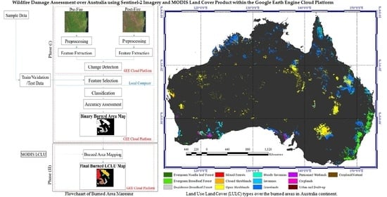
Wildfire Damage Assessment over Australia Using Sentinel-2 Imagery and MODIS Land Cover Product within the Google Earth Engine Cloud Platform


Abstract
:
1. Introduction
- (1)
- Many burned area products contain moderate spatial resolution. However, with the increasing availability of higher spatial resolution satellite imagery (e.g., Sentinel-2 with 10 (m) spatial resolution), there is potential to produce more detailed products in terms of spatial resolution.
- (2)
- Many RS methods for burned area mapping which are based on high-resolution imagery are complex and do not support the mapping of burned areas over large regions.
- (3)
- Although multi sensor-based methods for burned area mapping provide promising results, most of them are not computationally efficient.
- (4)
- A thresholding method which is applied in many research studies for discriminating burned from unburned areas does not provide accurate results for large regions, because burned areas at different regions depend on the characteristics of ecosystem and behavior of fire. Thus, a dynamic thresholding method should be developed to obtain high accuracies over different regions.
- (5)
- Many methods are based on the binary mapping (i.e., burned vs. unburned). However, estimation of the Land Use/Land Cover (LULC) over burned areas is necessary for many applications.
- (6)
- Many methods only use some specific spectral features. However, the potential of spatial features should be also comprehensively investigated to improve wildfire mapping and monitoring.
2. Materials and Methods
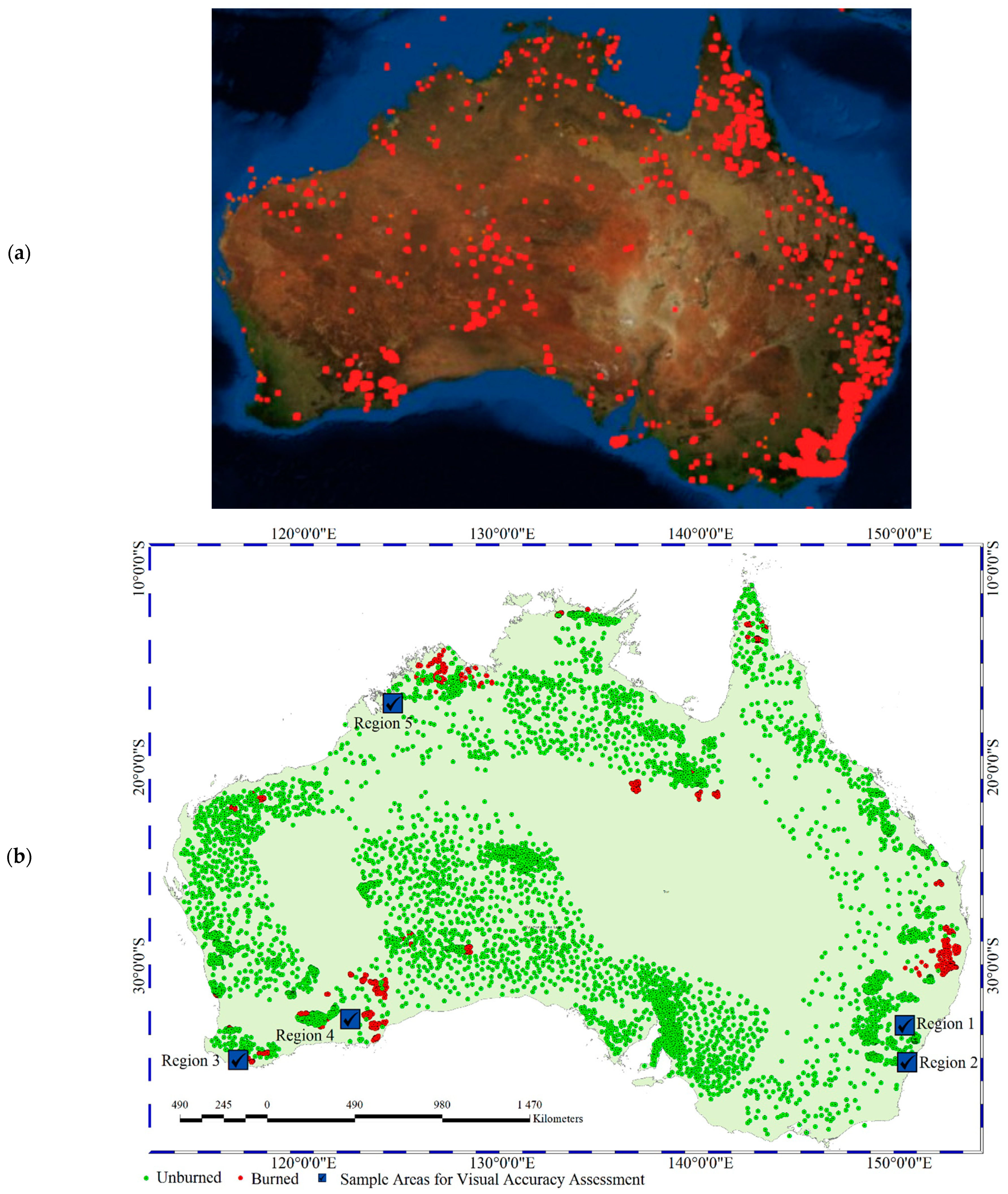
2.1. Study Area
2.2. Satellite Data
2.3. Reference Data
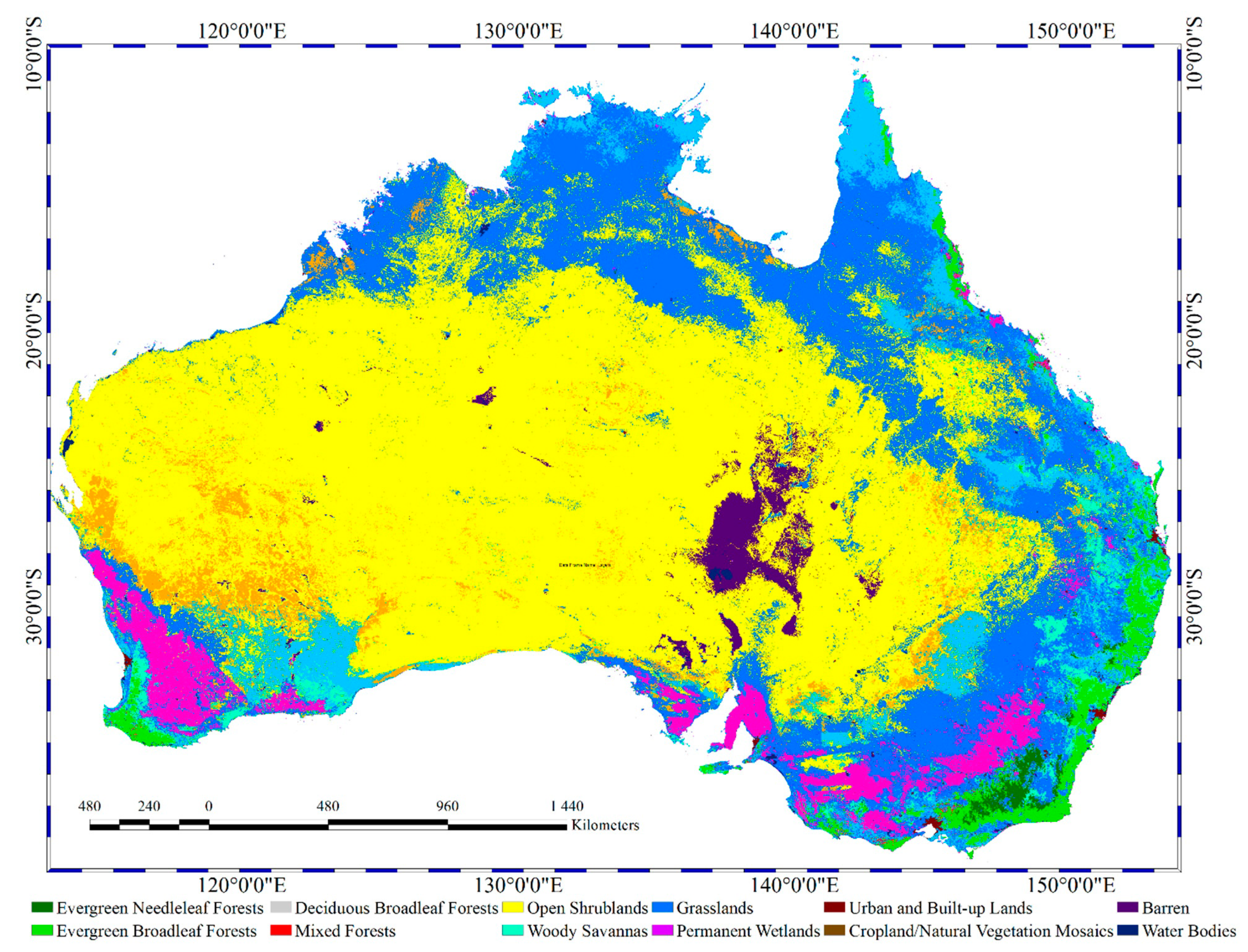
2.4. MODIS LULC Product
2.5. Landsat Burned Area Product
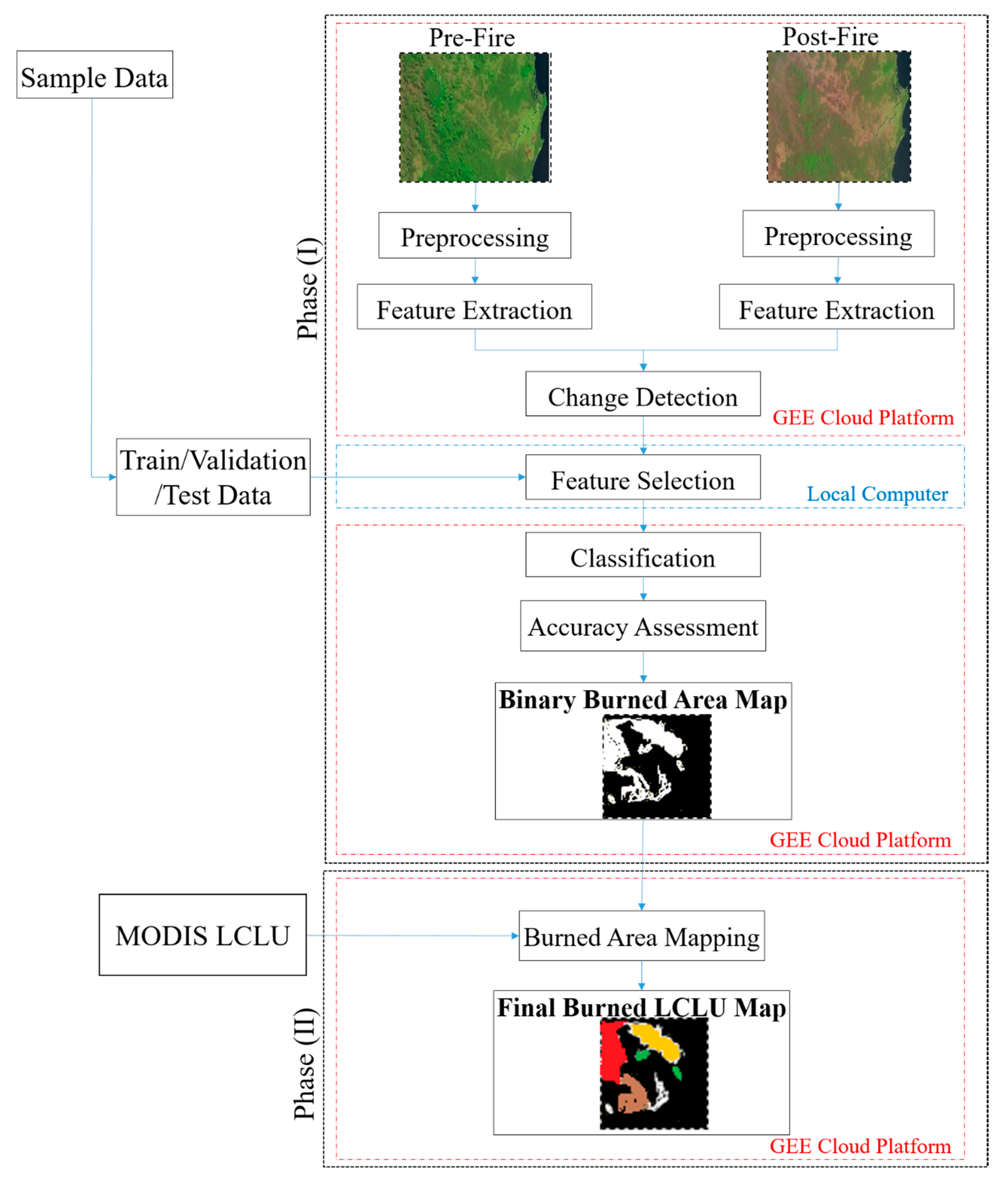
2.6. Proposed Method
2.6.1. Phase 1: Binary Burned Areas Mapping
Preprocessing
Feature Extraction
Change Detection
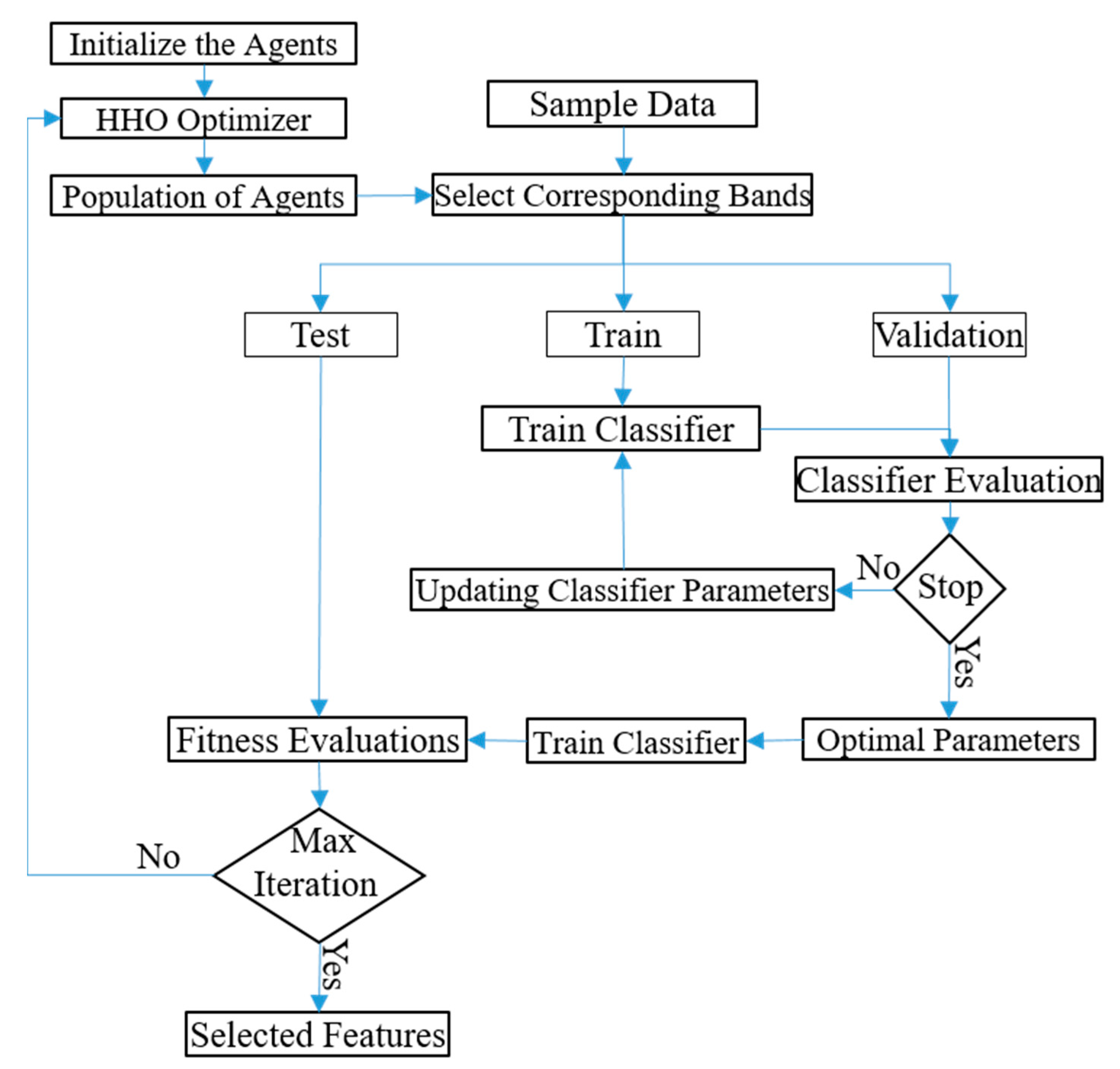
Feature Selection
Classification
RF Classifier
k-NN Classifier
SVM Classifier
Accuracy Assessment
2.6.2. Phase 2: Mapping LULC Types of Burned Areas
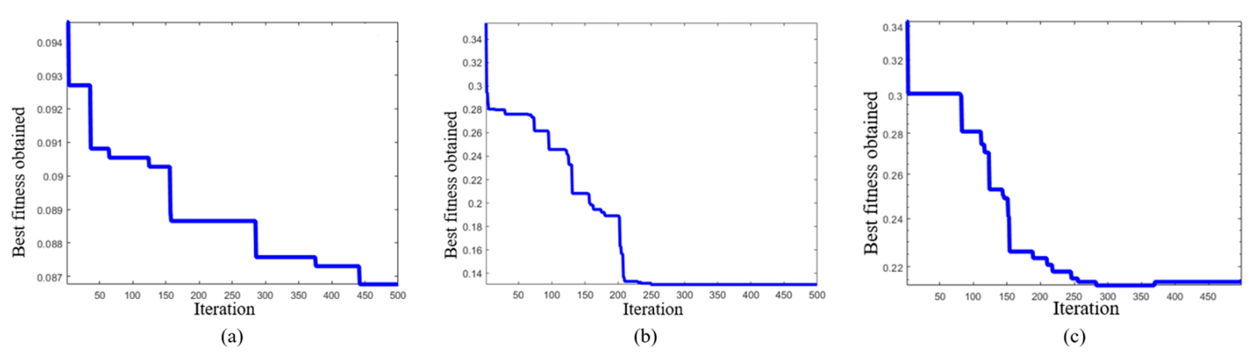
2.6.3. Parameter Setting and Feature Selection
3. Results
4. Discussion
5. Conclusions
Author Contributions
Funding
Institutional Review Board Statement
Informed Consent Statement
Data Availability Statement
Acknowledgments
Conflicts of Interest
Appendix A

| No. | Abbreviation | Index | Formula | Description | Reference |
|---|---|---|---|---|---|
| 1 | AFRI1 | Aerosol free vegetation index 1.6 | Vegetation Index | [64] | |
| 2 | AFRI2 | Aerosol free vegetation index 2.1 | Vegetation Index | [64] | |
| 3 | ARI | Anthocyanin reflectance index | Vegetation Index | [65] | |
| 4 | ARVI | Atmospherically resistant vegetation index | Vegetation Index | [66] | |
| 5 | ARVI2 | Atmospherically resistant vegetation index 2 | −0.18 + 1.17 ∗ | Vegetation Index | [66] |
| 6 | TSAVI | Adjusted transformed soil-adjusted vegetation index | Vegetation Index, a = 1.22, b = 0.03, X = 0.08 | [67] | |
| 7 | AVI | Ashburn vegetation index | Vegetation Index | [68] | |
| 8 | BNDVI | Blue-normalized difference vegetation index | Vegetation Index | [69] | |
| 9 | BRI | Browning reflectance index | Vegetation Index | [70] | |
| 10 | BWDRVI | Blue-wide dynamic range vegetation index | Vegetation Index | [71] | |
| 11 | CI | Color Index | Vegetation Index | [72] | |
| 12 | V | Vegetation | Vegetation Index | [73] | |
| 13 | CARI | Chlorophyll absorption ratio index | Vegetation Index, a = (Band5 − Band3)/150 b = B and 3 ∗ 550 ∗ a | [74] | |
| 14 | CCCI | Canopy chlorophyll content index | Vegetation Index | [75] | |
| 15 | CRI550 | Carotenoid reflectance index 550 | Vegetation Index | [76] | |
| 16 | CRI700 | Carotenoid reflectance index 700 | Vegetation Index | [76] | |
| 17 | CVI | Chlorophyll vegetation index | Vegetation Index | [77] | |
| 18 | Datt1 | Vegetation index proposed by Datt 1 | Vegetation Index | [78] | |
| 19 | Datt2 | Vegetation index proposed by Datt 2 | Vegetation Index | [79] | |
| 20 | Datt3 | Vegetation index proposed by Datt 3 | Vegetation Index | [79] | |
| 21 | DVI | Differenced vegetation index | Vegetation Index | [80] | |
| 22 | EPIcar | Eucalyptus pigment index for carotenoid | Vegetation Index | [79] | |
| 23 | EPIChla | Eucalyptus pigment index for chlorophyll a | Vegetation Index | [79] | |
| 24 | EPIChlab | Eucalyptus pigment index for chlorophyll a + b | Vegetation Index | [79] | |
| 25 | EPIChlb | Eucalyptus pigment index for chlorophyll b | Vegetation Index | [79] | |
| 26 | EVI | Enhanced vegetation index | Vegetation Index | [81] | |
| 27 | EVI2 | Enhanced vegetation index 2 | Vegetation Index | [82] | |
| 28 | EVI2.2 | Enhanced vegetation index 2.2 | Vegetation Index | [82] | |
| 29 | GARI | Green atmospherically resistant vegetation index | Vegetation Index | [83] | |
| 30 | GBNDVI | Green-Blue normalized difference vegetation index | Vegetation Index | [84] | |
| 31 | GDVI | Green difference vegetation index | Vegetation Index | [85] | |
| 32 | GEMI | Global environment monitoring index | Vegetation Index, n = | [86] | |
| 33 | GLI | Green leaf index | Vegetation Index | [87] | |
| 34 | GNDVI | Green normalized difference vegetation index | Vegetation Index | [83] | |
| 35 | GNDVI2 | Green normalized difference vegetation index 2 | Vegetation Index | [83] | |
| 36 | GOSAVI | Green optimized soil adjusted vegetation index | Vegetation Index | [88] | |
| 37 | GRNDVI | Green-Red normalized difference vegetation index | Vegetation Index | [89] | |
| 38 | GVMI | Global vegetation moisture index | Vegetation Index | [90] | |
| 39 | Hue | Hue | Vegetation Index | [91] | |
| 40 | IPVI | Infrared percentage vegetation index | Vegetation Index | [92] | |
| 41 | LCI | Leaf chlorophyll index | Vegetation Index | [78] | |
| 42 | Maccion | Vegetation index proposed by Maccioni | Vegetation Index | [93] | |
| 43 | MCARI | Modified chlorophyll absorption in reflectance index | Vegetation Index | [94] | |
| 44 | MTVI2 | Modified triangular vegetation index 2 | Vegetation Index | [95] | |
| 45 | MCARItoMTVI2 | MCARI/MTVI2 | Vegetation Index | [96] | |
| 46 | MCARItoOSAVI | MCARI/OSAVI | Vegetation Index | [95] | |
| 47 | MGVI | Green vegetation index proposed by Misra | Vegetation Index | [97] | |
| 49 | mNDVI | Modified normalized difference vegetation index | Vegetation Index | [98] | |
| 49 | MNSI | Non such index proposed by Misra | Vegetation Index | [97] | |
| 50 | MSAVI | Modified soil adjusted vegetation index | Vegetation Index | [99] | |
| 51 | MSAVI2 | Modified soil adjusted vegetation index 2 | Vegetation Index | [99] | |
| 52 | MSBI | Soil brightness index proposed by Misra | Vegetation Index | [97] | |
| 53 | MSR670 | Modified simple ratio 670/800 | Vegetation Index | [100] | |
| 54 | MSRNir/Red | Modified simple ratio NIR/red | Vegetation Index | [101] | |
| 55 | NBR | Normalized difference Nir/Swir normalized burn ratio | Vegetation Index | [102] | |
| 56 | ND774/677 | Normalized difference 774/677 | Vegetation Index | [103] | |
| 57 | NDII | Normalized difference infrared index | Vegetation Index | [104] | |
| 58 | NDRE | Normalized difference Red-edge | Vegetation Index | [105] | |
| 59 | NDSI | Normalized difference salinity index | Vegetation Index | [106] | |
| 60 | NDVI | Normalized difference vegetation index | Vegetation Index | [107] | |
| 61 | NDVI2 | Normalized difference vegetation index 2 | Vegetation Index | [85] | |
| 62 | NGRDI | Normalized green red difference index | Vegetation Index | [103] | |
| 63 | OSAVI | Optimized soil adjusted vegetation index | Vegetation Index | [108] | |
| 64 | PNDVI | Pan normalized difference vegetation index | Vegetation Index | [89] | |
| 65 | PVR | Photosynthetic vigor ratio | Vegetation Index | [109] | |
| 66 | RBNDVI | Red-Blue normalized difference vegetation index | Vegetation Index | [89] | |
| 67 | RDVI | Renormalized difference vegetation index | Vegetation Index | [110] | |
| 68 | REIP | Red-edge inflection point | 700 + 40 ∗ () | Vegetation Index | [111] |
| 69 | Rre | Reflectance at the inflexion point | Vegetation Index | [112] | |
| 70 | SAVI | Soil adjusted vegetation index | Vegetation Index | [113] | |
| 71 | SBL | Soil background line | Vegetation Index | [80] | |
| 72 | SIPI | Structure intensive pigment index | Vegetation Index | [114] | |
| 73 | SIWSI | Shortwave infrared water stress index | Vegetation Index | [115] | |
| 74 | SLAVI | Specific leaf area vegetation index | Vegetation Index | [116] | |
| 75 | TCARI | Transformed chlorophyll absorption Ratio | 3 ∗ (() − 0.2 ∗ ()()) | Vegetation Index | [94] |
| 76 | TCARItoOSAVI | TCARI/OSAVI | Vegetation Index | [108] | |
| 77 | TCI | Triangular chlorophyll index | 1.2 ∗ (() − 1.5 ∗ ()()) | Vegetation Index | [117] |
| 78 | TVI | Transformed vegetation index | Vegetation Index | [118] | |
| 79 | VARI700 | Visible atmospherically resistant index 700 | Vegetation Index | [119] | |
| 80 | VARIgreen | Visible atmospherically resistant index green | Vegetation Index | [119] | |
| 81 | VI700 | Vegetation index 700 | Vegetation Index | [120] | |
| 82 | WDRVI | Wide dynamic range vegetation index | Vegetation Index | [121] | |
| 83 | NDWI | Normalized Difference Water Index | Water Index | [122] | |
| 84 | MNDWI | Modified Normalized Difference Water Index | Water Index | [123] | |
| 85 | AWEInsh | Automated Water Extraction Index not dominant shadow | 4 ∗ () − (0.25 ∗ | Water Index | [50] |
| 86 | AWEIsh | Automated Water Extraction Index dominant shadow | + 2.5 ∗ − 1.5 ∗ () − 0.25 ∗ | Water Index | [50] |
| 87 | BI | Brightness Index | Bare Soil Index | [124] | |
| 88 | BI2 | Second Brightness Index | Bare Soil Index | [125] | |
| 89 | RI | Redness Index | Bare Soil Index | [72] | |
| 90 | BAIS2 | Burned Area Index for Sentinel-2 | ( | Burned Index | [33] |
| 91 | NBR | Normalized Burned Ratio Index | Burned Index | [102] |
Appendix B
| NO. | Abbreviation | Full Name | Formula | Description |
|---|---|---|---|---|
| 1 | ASM | Angular Second Moment | textural uniformity | |
| 2 | CONTRAST | Contrast | degree of spatial frequency | |
| 3 | CORR | Correlation | grey tone linear dependencies in the image | |
| 4 | VAR | Variance | Heterogeneity of image | |
| 5 | IDM | Inverse Difference Moment | image homogeneity | |
| 6 | SAVG | Sum Average | the mean of the gray level sum distribution of the image | |
| 7 | SVAR | Sum Variance | the dispersion of the gray level sum distribution of the image | |
| 8 | SENT | Sum Entropy | the disorder related to the gray level sum distribution of the image | |
| 9 | ENT | Entropy | Randomness of intensity distribution | |
| 10 | DVAR | Difference variance | the dispersion of the gray level difference distribution of the image | |
| 11 | DENT | Difference entropy | Degree of organization of gray level | |
| 12 | IMCORR1 | Information Measure of correlation 1 | dependency between two random variables | |
| 13 | IMCORR2 | Information Measure of correlation 2 | Linear dependence of gray level | |
| 14 | DISS | Dissimilarity | Total variation present | |
| 15 | INERTIA | Inertia | intensity contrast of image | |
| 16 | SHADE | Cluster Shade | Skewness of co-occurrence | |
| 17 | PROM | Cluster prominence | Asymmetry of image |
References
- Bokwa, A. Natural hazard. In Encyclopedia of Natural Hazards; Bobrowsky, P.T., Ed.; Springer: Dordrecht, The Netherlands, 2013; pp. 711–718. [Google Scholar] [CrossRef]
- Gibson, R.; Danaher, T.; Hehir, W.; Collins, L. A remote sensing approach to mapping fire severity in south-eastern Australia using sentinel 2 and random forest. Remote Sens. Environ. 2020, 240, 111702. [Google Scholar] [CrossRef]
- Collins, L.; McCarthy, G.; Mellor, A.; Newell, G.; Smith, L. Training data requirements for fire severity mapping using Landsat imagery and random forest. Remote Sens. Environ. 2020, 245, 111839. [Google Scholar] [CrossRef]
- Chuvieco, E.; Aguado, I.; Salas, J.; Garcia, M.; Yebra, M.; Oliva, P. Satellite Remote Sensing Contributions to Wildland Fire Science and Management. Curr. For. Rep. 2020, 6, 81–96. [Google Scholar] [CrossRef]
- Srivastava, S.; Kumar, A.S. Implications of intense biomass burning over Uttarakhand in April–May 2016. Nat. Hazards 2020, 101, 1–17. [Google Scholar] [CrossRef]
- Seydi, S.T.; Hasanlou, M. A new land-cover match-based change detection for hyperspectral imagery. Eur. J. Remote Sens. 2017, 50, 517–533. [Google Scholar] [CrossRef]
- Izadi, M.; Mohammadzadeh, A.; Haghighattalab, A. A new neuro-fuzzy approach for post-earthquake road damage assessment using GA and SVM classification from QuickBird satellite images. J. Indian Soc. Remote Sens. 2017, 45, 965–977. [Google Scholar] [CrossRef]
- Ghannadi, M.A.; SaadatSeresht, M.; Izadi, M.; Alebooye, S. Optimal texture image reconstruction method for improvement of SAR image matching. IET RadarSonar Navig. 2020, 14, 1229–1235. [Google Scholar] [CrossRef]
- Dragozi, E.; Gitas, I.Z.; Stavrakoudis, D.G.; Theocharis, J.B. Burned area mapping using support vector machines and the FuzCoC feature selection method on VHR IKONOS imagery. Remote Sens. 2014, 6, 12005–12036. [Google Scholar] [CrossRef] [Green Version]
- Oliva, P.; Schroeder, W. Assessment of VIIRS 375 m active fire detection product for direct burned area mapping. Remote Sens. Environ. 2015, 160, 144–155. [Google Scholar] [CrossRef]
- Chen, W.; Moriya, K.; Sakai, T.; Koyama, L.; Cao, C. Mapping a burned forest area from Landsat TM data by multiple methods. Geomat. Nat. Hazards Risk 2016, 7, 384–402. [Google Scholar] [CrossRef] [Green Version]
- Hawbaker, T.J.; Vanderhoof, M.K.; Beal, Y.-J.; Takacs, J.D.; Schmidt, G.L.; Falgout, J.T.; Williams, B.; Fairaux, N.M.; Caldwell, M.K.; Picotte, J.J. Mapping burned areas using dense time-series of Landsat data. Remote Sens. Environ. 2017, 198, 504–522. [Google Scholar] [CrossRef]
- Pereira, A.A.; Pereira, J.; Libonati, R.; Oom, D.; Setzer, A.W.; Morelli, F.; Machado-Silva, F.; De Carvalho, L.M.T. Burned area mapping in the Brazilian Savanna using a one-class support vector machine trained by active fires. Remote Sens. 2017, 9, 1161. [Google Scholar] [CrossRef] [Green Version]
- Roteta, E.; Bastarrika, A.; Padilla, M.; Storm, T.; Chuvieco, E. Development of a Sentinel-2 burned area algorithm: Generation of a small fire database for sub-Saharan Africa. Remote Sens. Environ. 2019, 222, 1–17. [Google Scholar] [CrossRef]
- Ba, R.; Song, W.; Li, X.; Xie, Z.; Lo, S. Integration of multiple spectral indices and a neural network for burned area mapping based on MODIS data. Remote Sens. 2019, 11, 326. [Google Scholar] [CrossRef] [Green Version]
- Woźniak, E.; Aleksandrowicz, S. Self-Adjusting Thresholding for Burnt Area Detection Based on Optical Images. Remote Sens. 2019, 11, 2669. [Google Scholar] [CrossRef] [Green Version]
- Otón, G.; Ramo, R.; Lizundia-Loiola, J.; Chuvieco, E. Global Detection of Long-Term (1982–2017) Burned Area with AVHRR-LTDR Data. Remote Sens. 2019, 11, 2079. [Google Scholar] [CrossRef] [Green Version]
- Liu, M.; Popescu, S.; Malambo, L. Feasibility of Burned Area Mapping Based on ICESAT− 2 Photon Counting Data. Remote Sens. 2020, 12, 24. [Google Scholar] [CrossRef] [Green Version]
- Gorelick, N.; Hancher, M.; Dixon, M.; Ilyushchenko, S.; Thau, D.; Moore, R. Google Earth Engine: Planetary-scale geospatial analysis for everyone. Remote Sens. Environ. 2017, 202, 18–27. [Google Scholar] [CrossRef]
- Amani, M.; Ghorbanian, A.; Ahmadi, S.A.; Kakooei, M.; Moghimi, A.; Mirmazloumi, S.M.; Moghaddam, S.H.A.; Mahdavi, S.; Ghahremanloo, M.; Parsian, S. Google earth engine cloud computing platform for remote sensing big data applications: A comprehensive review. IEEE J. Sel. Top. Appl. Earth Obs. Remote Sens. 2020. [Google Scholar] [CrossRef]
- Long, T.; Zhang, Z.; He, G.; Jiao, W.; Tang, C.; Wu, B.; Zhang, X.; Wang, G.; Yin, R. 30 m Resolution Global Annual Burned Area Mapping Based on Landsat Images and Google Earth Engine. Remote Sens. 2019, 11, 489. [Google Scholar] [CrossRef] [Green Version]
- Zhang, Z.; He, G.; Long, T.; Tang, C.; Wei, M.; Wang, W.; Wang, G. Spatial Pattern Analysis of Global Burned Area in 2005 Based on Landsat Satellite Images. In Proceedings of IOP Conference Series: Earth and Environmental Science; IOP Publishing: Philadelphia, PA, USA, 2020; p. 012078. [Google Scholar]
- Barboza Castillo, E.; Turpo Cayo, E.Y.; de Almeida, C.M.; Salas López, R.; Rojas Briceño, N.B.; Silva López, J.O.; Barrena Gurbillón, M.Á.; Oliva, M.; Espinoza-Villar, R. Monitoring Wildfires in the Northeastern Peruvian Amazon Using Landsat-8 and Sentinel-2 Imagery in the GEE Platform. ISPRS Int. J. Geo-Inf. 2020, 9, 564. [Google Scholar] [CrossRef]
- Ehsani, M.R.; Arevalo, J.; Risanto, C.B.; Javadian, M.; Devine, C.J.; Arabzadeh, A.; Venegas-Quiñones, H.L.; Dell’Oro, A.P.; Behrangi, A. 2019–2020 Australia Fire and Its Relationship to Hydroclimatological and Vegetation Variabilities. Water 2020, 12, 3067. [Google Scholar] [CrossRef]
- Available online: http://www.bom.gov.au/climate/ (accessed on 22 December 2020).
- Drusch, M.; Del Bello, U.; Carlier, S.; Colin, O.; Fernandez, V.; Gascon, F.; Hoersch, B.; Isola, C.; Laberinti, P.; Martimort, P. Sentinel-2: ESA’s optical high-resolution mission for GMES operational services. Remote Sens. Environ. 2012, 120, 25–36. [Google Scholar] [CrossRef]
- Available online: https://www.ktnv.com/ (accessed on 13 November 2020).
- Chen, Y.; Song, L.; Liu, Y.; Yang, L.; Li, D. A Review of the Artificial Neural Network Models for Water Quality Prediction. Appl. Sci. 2020, 10, 5776. [Google Scholar] [CrossRef]
- Sulla-Menashe, D.; Friedl, M.A. User Guide to Collection 6 MODIS Land Cover (MCD12Q1 and MCD12C1) Product; USGS: Reston, VA, USA, 2018; pp. 1–18.
- Available online: https://www.usgs.gov/core-science-systems/nli/landsat/landsat-burned-area (accessed on 13 November 2020).
- Xue, J.; Su, B. Significant remote sensing vegetation indices: A review of developments and applications. J. Sens. 2017, 2017, 1353691. [Google Scholar] [CrossRef] [Green Version]
- Liu, S.; Zheng, Y.; Dalponte, M.; Tong, X. A novel fire index-based burned area change detection approach using Landsat-8 OLI data. Eur. J. Remote Sens. 2020, 53, 104–112. [Google Scholar] [CrossRef] [Green Version]
- Filipponi, F. BAIS2: Burned area index for Sentinel-2. Proceedings 2018, 2, 364. [Google Scholar] [CrossRef] [Green Version]
- Conners, R.W.; Trivedi, M.M.; Harlow, C.A. Segmentation of a high-resolution urban scene using texture operators. Comput. Vis. Graph. Image Process. 1984, 25, 273–310. [Google Scholar] [CrossRef]
- Mahdavi, S.; Salehi, B.; Amani, M.; Granger, J.; Brisco, B.; Huang, W. A dynamic classification scheme for mapping spectrally similar classes: Application to wetland classification. Int. J. Appl. Earth Obs. Geoinf. 2019, 83, 101914. [Google Scholar] [CrossRef]
- Heidari, A.A.; Mirjalili, S.; Faris, H.; Aljarah, I.; Mafarja, M.; Chen, H. Harris hawks optimization: Algorithm and applications. Future Gener. Comput. Syst. 2019, 97, 849–872. [Google Scholar] [CrossRef]
- Houssein, E.H.; Hosney, M.E.; Oliva, D.; Mohamed, W.M.; Hassaballah, M. A novel hybrid Harris hawks optimization and support vector machines for drug design and discovery. Comput. Chem. Eng. 2020, 133, 106656. [Google Scholar] [CrossRef]
- Amani, M.; Mahdavi, S.; Berard, O. Supervised wetland classification using high spatial resolution optical, SAR, and LiDAR imagery. J. Appl. Remote Sens. 2020, 14, 024502. [Google Scholar] [CrossRef]
- Mahdavi, S.; Salehi, B.; Amani, M.; Granger, J.E.; Brisco, B.; Huang, W.; Hanson, A. Object-based classification of wetlands in Newfoundland and Labrador using multi-temporal PolSAR data. Can. J. Remote Sens. 2017, 43, 432–450. [Google Scholar] [CrossRef]
- Ghorbanian, A.; Kakooei, M.; Amani, M.; Mahdavi, S.; Mohammadzadeh, A.; Hasanlou, M. Improved land cover map of Iran using Sentinel imagery within Google Earth Engine and a novel automatic workflow for land cover classification using migrated training samples. ISPRS J. Photogramm. Remote Sens. 2020, 167, 276–288. [Google Scholar] [CrossRef]
- Amani, M.; Mahdavi, S.; Afshar, M.; Brisco, B.; Huang, W.; Mohammad Javad Mirzadeh, S.; White, L.; Banks, S.; Montgomery, J.; Hopkinson, C. Canadian wetland inventory using Google Earth engine: The first map and preliminary results. Remote Sens. 2019, 11, 842. [Google Scholar] [CrossRef] [Green Version]
- Liaw, A.; Wiener, M. Classification and regression by randomForest. R News 2002, 2, 18–22. [Google Scholar]
- Amani, M.; Salehi, B.; Mahdavi, S.; Granger, J.E.; Brisco, B.; Hanson, A. Wetland classification using multi-source and multi-temporal optical remote sensing data in Newfoundland and Labrador, Canada. Can. J. Remote Sens. 2017, 43, 360–373. [Google Scholar] [CrossRef]
- Fu, K.-S. Applications of Pattern Recognition; CRC Press: Boca Raton, FL, USA, 2019. [Google Scholar]
- Amani, M.; Salehi, B.; Mahdavi, S.; Brisco, B.; Shehata, M. A Multiple Classifier System to improve mapping complex land covers: A case study of wetland classification using SAR data in Newfoundland, Canada. Int. J. Remote Sens. 2018, 39, 7370–7383. [Google Scholar] [CrossRef]
- Vapnik, V. The Nature of Statistical Learning Theory; Springer Science & Business Media: Berlin/Heidelberg, Germany, 2013. [Google Scholar]
- Yekkehkhany, B.; Safari, A.; Homayouni, S.; Hasanlou, M. A comparison study of different kernel functions for SVM-based classification of multi-temporal polarimetry SAR data. Int. Arch. Photogramm. Remote Sens. Spat. Inf. Sci. 2014, 40, 281. [Google Scholar] [CrossRef] [Green Version]
- Seydi, S.T.; Hasanlou, M.; Amani, M. A New End-to-End Multi-Dimensional CNN Framework for Land Cover/Land Use Change Detection in Multi-Source Remote Sensing Datasets. Remote Sens. 2020, 12, 2010. [Google Scholar] [CrossRef]
- Wang, Q.; Yuan, Z.; Du, Q.; Li, X. GETNET: A general end-to-end 2-D CNN framework for hyperspectral image change detection. IEEE Trans. Geosci. Remote Sens. 2018, 57, 3–13. [Google Scholar] [CrossRef] [Green Version]
- Feyisa, G.L.; Meilby, H.; Fensholt, R.; Proud, S.R. Automated Water Extraction Index: A new technique for surface water mapping using Landsat imagery. Remote Sens. Environ. 2014, 140, 23–35. [Google Scholar] [CrossRef]
- Bastarrika, A.; Chuvieco, E.; Martin, M.P. Mapping burned areas from Landsat TM/ETM+ data with a two-phase algorithm: Balancing omission and commission errors. Remote Sens. Environ. 2011, 115, 1003–1012. [Google Scholar] [CrossRef]
- Fernández-Manso, A.; Quintano, C. A Synergetic Approach to Burned Area Mapping Using Maximum Entropy Modeling Trained with Hyperspectral Data and VIIRS Hotspots. Remote Sens. 2020, 12, 858. [Google Scholar] [CrossRef] [Green Version]
- Shin, J.-i.; Seo, W.-w.; Kim, T.; Park, J.; Woo, C.-s. Using UAV multispectral images for classification of forest burn severity—A case study of the 2019 Gangneung forest fire. Forests 2019, 10, 1025. [Google Scholar] [CrossRef] [Green Version]
- Fraser, R.H.; Van der Sluijs, J.; Hall, R.J. Calibrating satellite-based indices of burn severity from UAV-derived metrics of a burned boreal forest in NWT, Canada. Remote Sens. 2017, 9, 279. [Google Scholar] [CrossRef] [Green Version]
- Calin, M.A.; Parasca, S.V.; Savastru, R.; Manea, D. Characterization of burns using hyperspectral imaging technique–A preliminary study. Burns 2015, 41, 118–124. [Google Scholar] [CrossRef]
- Schepers, L.; Haest, B.; Veraverbeke, S.; Spanhove, T.; Vanden Borre, J.; Goossens, R. Burned area detection and burn severity assessment of a heathland fire in Belgium using airborne imaging spectroscopy (APEX). Remote Sens. 2014, 6, 1803–1826. [Google Scholar] [CrossRef] [Green Version]
- Yin, C.; He, B.; Yebra, M.; Quan, X.; Edwards, A.C.; Liu, X.; Liao, Z.; Luo, K. Burn Severity Estimation in Northern Australia Tropical Savannas Using Radiative Transfer Model and Sentinel-2 Data. In Proceedings of the IGARSS 2019–2019 IEEE International Geoscience and Remote Sensing Symposium, Yokohama, Japan, 28 July–2 August 2019; pp. 6712–6715. [Google Scholar]
- Santana, N.C.; de Carvalho Júnior, O.A.; Gomes, R.A.T.; Guimarães, R.F. Burned-area detection in amazonian environments using standardized time series per pixel in MODIS data. Remote Sens. 2018, 10, 1904. [Google Scholar] [CrossRef] [Green Version]
- Simon, M.; Plummer, S.; Fierens, F.; Hoelzemann, J.J.; Arino, O. Burnt area detection at global scale using ATSR-2: The GLOBSCAR products and their qualification. J. Geophys. Res. Atmos. 2004, 109. [Google Scholar] [CrossRef]
- De Araújo, F.M.; Ferreira, L.G. Satellite-based automated burned area detection: A performance assessment of the MODIS MCD45A1 in the Brazilian savanna. Int. J. Appl. Earth Obs. Geoinf. 2015, 36, 94–102. [Google Scholar] [CrossRef]
- Knopp, L.; Wieland, M.; Rättich, M.; Martinis, S. A Deep Learning Approach for Burned Area Segmentation with Sentinel-2 Data. Remote Sens. 2020, 12, 2422. [Google Scholar] [CrossRef]
- Pinto, M.M.; Libonati, R.; Trigo, R.M.; Trigo, I.F.; DaCamara, C.C. A deep learning approach for mapping and dating burned areas using temporal sequences of satellite images. ISPRS J. Photogramm. Remote Sens. 2020, 160, 260–274. [Google Scholar] [CrossRef]
- Ban, Y.; Zhang, P.; Nascetti, A.; Bevington, A.R.; Wulder, M.A. Near Real-Time Wildfire Progression Monitoring with Sentinel-1 SAR Time Series and Deep Learning. Sci. Rep. 2020, 10, 1–15. [Google Scholar] [CrossRef] [PubMed] [Green Version]
- Karnieli, A.; Kaufman, Y.J.; Remer, L.; Wald, A. AFRI—Aerosol free vegetation index. Remote Sens. Environ. 2001, 77, 10–21. [Google Scholar] [CrossRef]
- Gitelson, A.A.; Chivkunova, O.B.; Merzlyak, M.N. Nondestructive estimation of anthocyanins and chlorophylls in anthocyanic leaves. Am. J. Bot. 2009, 96, 1861–1868. [Google Scholar] [CrossRef]
- Kaufman, Y.J.; Tanre, D. Atmospherically resistant vegetation index (ARVI) for EOS-MODIS. IEEE Trans. Geosci. Remote Sens. 1992, 30, 261–270. [Google Scholar] [CrossRef]
- Baret, F.; Guyot, G. Potentials and limits of vegetation indices for LAI and APAR assessment. Remote Sens. Environ. 1991, 35, 161–173. [Google Scholar] [CrossRef]
- Ashburn, P. The vegetative index number and crop identification. In Proceedings of the Technical Sessions of the LACIE Symposium, Houston, TX, USA, 23–26 October 1978; pp. 843–855. [Google Scholar]
- Yang, C.; Everitt, J.H.; Bradford, J.M. Airborne hyperspectral imagery and linear spectral unmixing for mapping variation in crop yield. Precis. Agric. 2007, 8, 279–296. [Google Scholar] [CrossRef]
- Chivkunova, O.B.; Solovchenko, A.E.; Sokolova, S.; Merzlyak, M.N.; Reshetnikova, I.; Gitelson, A.A. Reflectance spectral features and detection of superficial scald–induced browning in storing apple fruit. Russ. J. Phytopathol. 2001, 2, 73–77. [Google Scholar]
- Hancock, D.W.; Dougherty, C.T. Relationships between blue-and red-based vegetation indices and leaf area and yield of alfalfa. Crop Sci. 2007, 47, 2547–2556. [Google Scholar] [CrossRef]
- Pouget, M.; Madeira, J.; Le Floch, E.; Kamal, S. Caracteristiques spectrales des surfaces sableuses de la region cotiere nord-ouest de l’Egypte: Application aux donnees satellitaires SPOT. In Journee de Teledetection Caractérisation et Suivi des Milieux Terrestres en Régions Arides et Tropicales; ORSTOM: Paris, France, 1990; Volume 12, pp. 27–39. [Google Scholar]
- Jordan, C.F. Derivation of leaf-area index from quality of light on the forest floor. Ecology 1969, 50, 663–666. [Google Scholar] [CrossRef]
- Kim, M.S.; Daughtry, C.; Chappelle, E.; McMurtrey, J.; Walthall, C. The use of high spectral resolution bands for estimating absorbed photosynthetically active radiation (A par). In Proceedings of the 6th International Symposium on Physical Measurements and Signatures in Remote Sensing, Phoenix, AZ, USA, 1 January 1994; CNES: Paris, France, 1994. [Google Scholar]
- El-Shikha, D.M.; Barnes, E.M.; Clarke, T.R.; Hunsaker, D.J.; Haberland, J.A.; Pinter, P., Jr.; Waller, P.M.; Thompson, T.L. Remote sensing of cotton nitrogen status using the canopy chlorophyll content index (CCCI). Trans. Asabe 2008, 51, 73–82. [Google Scholar] [CrossRef]
- Gitelson, A.A.; Merzlyak, M.N.; Chivkunova, O.B. Optical properties and nondestructive estimation of anthocyanin content in plant leaves. Photochem. Photobiol. 2001, 74, 38–45. [Google Scholar] [CrossRef]
- Hunt, E.R., Jr.; Daughtry, C.; Eitel, J.U.; Long, D.S. Remote sensing leaf chlorophyll content using a visible band index. Agron. J. 2011, 103, 1090–1099. [Google Scholar] [CrossRef] [Green Version]
- Datt, B. Remote sensing of water content in Eucalyptus leaves. Aust. J. Bot. 1999, 47, 909–923. [Google Scholar] [CrossRef]
- Datt, B. Remote sensing of chlorophyll a, chlorophyll b, chlorophyll a + b, and total carotenoid content in eucalyptus leaves. Remote Sens. Environ. 1998, 66, 111–121. [Google Scholar] [CrossRef]
- Richardson, A.J.; Wiegand, C. Distinguishing vegetation from soil background information. Photogramm. Eng. Remote Sens. 1977, 43, 1541–1552. [Google Scholar]
- Huete, A.; Didan, K.; Miura, T.; Rodriguez, E.P.; Gao, X.; Ferreira, L.G. Overview of the radiometric and biophysical performance of the MODIS vegetation indices. Remote Sens. Environ. 2002, 83, 195–213. [Google Scholar] [CrossRef]
- Miura, T.; Yoshioka, H.; Fujiwara, K.; Yamamoto, H. Inter-comparison of ASTER and MODIS surface reflectance and vegetation index products for synergistic applications to natural resource monitoring. Sensors 2008, 8, 2480–2499. [Google Scholar] [CrossRef] [Green Version]
- Gitelson, A.A.; Kaufman, Y.J.; Merzlyak, M.N. Use of a green channel in remote sensing of global vegetation from EOS-MODIS. Remote Sens. Environ. 1996, 58, 289–298. [Google Scholar] [CrossRef]
- Wang, F.; Huang, J.; Chen, L. Development of a vegetation index for estimation of leaf area index based on simulation modeling. J. Plant Nutr. 2010, 33, 328–338. [Google Scholar] [CrossRef]
- Tucker, C.J.; Elgin, J., Jr.; McMurtrey, J., III; Fan, C. Monitoring corn and soybean crop development with hand-held radiometer spectral data. Remote Sens. Environ. 1979, 8, 237–248. [Google Scholar] [CrossRef]
- Pinty, B.; Verstraete, M. GEMI: A non-linear index to monitor global vegetation from satellites. Vegetatio 1992, 101, 15–20. [Google Scholar] [CrossRef]
- Gobron, N.; Pinty, B.; Verstraete, M.M.; Widlowski, J.-L. Advanced vegetation indices optimized for up-coming sensors: Design, performance, and applications. IEEE Trans. Geosci. Remote Sens. 2000, 38, 2489–2505. [Google Scholar]
- Rondeaux, G.; Steven, M.; Baret, F. Optimization of soil-adjusted vegetation indices. Remote Sens. Environ. 1996, 55, 95–107. [Google Scholar] [CrossRef]
- Wang, F.-M.; Huang, J.-F.; Tang, Y.-L.; Wang, X.-Z. New vegetation index and its application in estimating leaf area index of rice. Rice Sci. 2007, 14, 195–203. [Google Scholar] [CrossRef]
- Glenn, E.P.; Nagler, P.L.; Huete, A.R. Vegetation index methods for estimating evapotranspiration by remote sensing. Surv. Geophys. 2010, 31, 531–555. [Google Scholar] [CrossRef]
- Escadafal, R.; Belghith, A.; Ben-Moussa, H. Indices spectraux pour la dégradation des milieux naturels en Tunisie aride. In Proceedings of the 6ème Symp. Int.“Mesures Physiques et Signatures en Télédétection”, Val d’Isere, France, 17–21 January 1994; pp. 253–259. [Google Scholar]
- Crippen, R.E. Calculating the vegetation index faster. Remote Sens. Environ. 1990, 34, 71–73. [Google Scholar] [CrossRef]
- Maccioni, A.; Agati, G.; Mazzinghi, P. New vegetation indices for remote measurement of chlorophylls based on leaf directional reflectance spectra. J. Photochem. Photobiol. B Biol. 2001, 61, 52–61. [Google Scholar] [CrossRef]
- Daughtry, C.; Walthall, C.; Kim, M.; De Colstoun, E.B.; McMurtrey, J., III. Estimating corn leaf chlorophyll concentration from leaf and canopy reflectance. Remote Sens. Environ. 2000, 74, 229–239. [Google Scholar] [CrossRef]
- Haboudane, D.; Miller, J.R.; Pattey, E.; Zarco-Tejada, P.J.; Strachan, I.B. Hyperspectral vegetation indices and novel algorithms for predicting green LAI of crop canopies: Modeling and validation in the context of precision agriculture. Remote Sens. Environ. 2004, 90, 337–352. [Google Scholar] [CrossRef]
- Eitel, J.; Long, D.; Gessler, P.; Smith, A. Using in-situ measurements to evaluate the new RapidEye™ satellite series for prediction of wheat nitrogen status. Int. J. Remote Sens. 2007, 28, 4183–4190. [Google Scholar] [CrossRef]
- Misra, P.; Wheeler, S.G.; Oliver, R.E. Kauth-Thomas brightness and greenness axes. Contract NASA 1977, 23–46. [Google Scholar]
- Main, R.; Cho, M.A.; Mathieu, R.; O’Kennedy, M.M.; Ramoelo, A.; Koch, S. An investigation into robust spectral indices for leaf chlorophyll estimation. ISPRS J. Photogramm. Remote Sens. 2011, 66, 751–761. [Google Scholar] [CrossRef]
- Qi, J.; Chehbouni, A.; Huete, A.R.; Kerr, Y.H.; Sorooshian, S. A modified soil adjusted vegetation index. Remote Sens. Environ. 1994, 48, 119–126. [Google Scholar] [CrossRef]
- Chen, J.M. Evaluation of vegetation indices and a modified simple ratio for boreal applications. Can. J. Remote Sens. 1996, 22, 229–242. [Google Scholar] [CrossRef]
- Chen, J.M.; Cihlar, J. Retrieving leaf area index of boreal conifer forests using Landsat TM images. Remote Sens. Environ. 1996, 55, 153–162. [Google Scholar] [CrossRef]
- Key, C.; Benson, N. Landscape Assessment: Ground Measure of Severity, the Composite Burn Index; and Remote Sensing of Severity, the Normalized Burn Ratio; FIREMON: Fire Effects Monitoring and Inventory System; USDA Forest Service, Rocky Mountain Research Station: Fort Collins, CO, USA, 2005; Volume 2004.
- Zarco-Tejada, P.J.; Miller, J.R.; Noland, T.L.; Mohammed, G.H.; Sampson, P.H. Scaling-up and model inversion methods with narrowband optical indices for chlorophyll content estimation in closed forest canopies with hyperspectral data. IEEE Trans. Geosci. Remote Sens. 2001, 39, 1491–1507. [Google Scholar] [CrossRef] [Green Version]
- Klemas, V.; Smart, R. The Influence of Soil Salinity, Growth Form, and Leaf Moisture on-the Spectral Radiance of. Photogramm. Eng. Remote Sens. 1983, 49, 77–83. [Google Scholar]
- Barnes, E.; Clarke, T.; Richards, S.; Colaizzi, P.; Haberland, J.; Kostrzewski, M.; Waller, P.; Choi, C.; Riley, E.; Thompson, T. Coincident detection of crop water stress, nitrogen status and canopy density using ground based multispectral data. In Proceedings of the Fifth International Conference on Precision Agriculture, Bloomington, MN, USA, 16–19 July 2000. [Google Scholar]
- Dehni, A.; Lounis, M. Remote sensing techniques for salt affected soil mapping: Application to the Oran region of Algeria. Procedia Eng. 2012, 33, 188–198. [Google Scholar] [CrossRef] [Green Version]
- Tucker, C.J. Red and photographic infrared linear combinations for monitoring vegetation. Remote Sens. Environ. 1979, 8, 127–150. [Google Scholar] [CrossRef] [Green Version]
- Haboudane, D.; Miller, J.R.; Tremblay, N.; Zarco-Tejada, P.J.; Dextraze, L. Integrated narrow-band vegetation indices for prediction of crop chlorophyll content for application to precision agriculture. Remote Sens. Environ. 2002, 81, 416–426. [Google Scholar] [CrossRef]
- Metternicht, G. Vegetation indices derived from high-resolution airborne videography for precision crop management. Int. J. Remote Sens. 2003, 24, 2855–2877. [Google Scholar] [CrossRef]
- Broge, N.H.; Leblanc, E. Comparing prediction power and stability of broadband and hyperspectral vegetation indices for estimation of green leaf area index and canopy chlorophyll density. Remote Sens. Environ. 2001, 76, 156–172. [Google Scholar] [CrossRef]
- Herrmann, I.; Pimstein, A.; Karnieli, A.; Cohen, Y.; Alchanatis, V.; Bonfil, D. LAI assessment of wheat and potato crops by VENμS and Sentinel-2 bands. Remote Sens. Environ. 2011, 115, 2141–2151. [Google Scholar] [CrossRef]
- Clevers, J.; De Jong, S.; Epema, G.; Van Der Meer, F.; Bakker, W.; Skidmore, A.; Scholte, K. Derivation of the red edge index using the MERIS standard band setting. Int. J. Remote Sens. 2002, 23, 3169–3184. [Google Scholar] [CrossRef] [Green Version]
- Huete, A.R. A soil-adjusted vegetation index (SAVI). Remote Sensing of Environment. Remote Sens. Environ. 1988, 25, 295–309. [Google Scholar] [CrossRef]
- Penuelas, J.; Baret, F.; Filella, I. Semi-empirical indices to assess carotenoids/chlorophyll a ratio from leaf spectral reflectance. Photosynthetica 1995, 31, 221–230. [Google Scholar]
- Fensholt, R.; Sandholt, I. Derivation of a shortwave infrared water stress index from MODIS near-and shortwave infrared data in a semiarid environment. Remote Sens. Environ. 2003, 87, 111–121. [Google Scholar] [CrossRef]
- Lymburner, L.; Beggs, P.J.; Jacobson, C.R. Estimation of canopy-average surface-specific leaf area using Landsat TM data. Photogramm. Eng. Remote Sens. 2000, 66, 183–192. [Google Scholar]
- Haboudane, D.; Tremblay, N.; Miller, J.R.; Vigneault, P. Remote estimation of crop chlorophyll content using spectral indices derived from hyperspectral data. IEEE Trans. Geosci. Remote Sens. 2008, 46, 423–437. [Google Scholar] [CrossRef]
- Rousel, J.; Haas, R.; Schell, J.; Deering, D. Monitoring vegetation systems in the great plains with ERTS. In Proceedings of the Third Earth Resources Technology Satellite—1 Symposium, Washington, DC, USA, 10–14 December 1973; pp. 309–317. [Google Scholar]
- Gitelson, A.A.; Merzlyak, M.; Zur, Y.; Stark, R.; Gritz, U. Non-destructive and remote sensing techniques for estimation of vegetation status. In Proceedings of the 3rd European Conference on Precision Agriculture, Montpelier, France, 18–20 June 2001. [Google Scholar]
- Gitelson, A.A.; Kaufman, Y.J.; Stark, R.; Rundquist, D. Novel algorithms for remote estimation of vegetation fraction. Remote Sens. Environ. 2002, 80, 76–87. [Google Scholar] [CrossRef] [Green Version]
- Gitelson, A.A. Wide dynamic range vegetation index for remote quantification of biophysical characteristics of vegetation. J. Plant Physiol. 2004, 161, 165–173. [Google Scholar] [CrossRef] [Green Version]
- McFeeters, S.K. The use of the Normalized Difference Water Index (NDWI) in the delineation of open water features. Int. J. Remote Sens. 1996, 17, 1425–1432. [Google Scholar] [CrossRef]
- Xu, H. Modification of normalised difference water index (NDWI) to enhance open water features in remotely sensed imagery. Int. J. Remote Sens. 2006, 27, 3025–3033. [Google Scholar] [CrossRef]
- Escadafal, R.; Bacha, S. Strategy for the dynamic study of desertification. In Surveillance des sols dans l’environnement par télédétection et systèmes d’information géogr; ORSTOM Editions: Paris, France, 1996; pp. 19–34. [Google Scholar]
- Escadafal, R. Remote sensing of arid soil surface color with Landsat thematic mapper. Adv. Space Res. 1989, 9, 159–163. [Google Scholar] [CrossRef]


| Class | Number of Samples | Training | Validation | Test |
|---|---|---|---|---|
| Burned | 5485 | 2806 | 877 | 1802 |
| Unburned | 5433 | 2654 | 870 | 1909 |
| Number | Name Class | Area (km2) | Percent (%) |
|---|---|---|---|
| 1 | Evergreen Needle leaf Forests | 22,445 | 0.41 |
| 2 | Evergreen Broadleaf Forests | 113,805 | 2.10 |
| 3 | Deciduous Needle leaf Forests | 0.2 | 0 |
| 4 | Deciduous Broadleaf Forests | 795 | 0.01 |
| 5 | Mixed Forests | 3100 | 0.05 |
| 6 | Closed Shrublands | 183,366 | 3.38 |
| 7 | Open Shrublands | 2,336,706 | 43.18 |
| 8 | Woody Savannas | 91,285 | 1.68 |
| 9 | Savannas | 474,943 | 8.77 |
| 10 | Grasslands | 1,816,831 | 33.57 |
| 11 | Permanent Wetlands | 8134 | 0.15 |
| 12 | Croplands | 162,705 | 3.00 |
| 13 | Urban and Built-up Lands | 6843 | 0.12 |
| 14 | Cropland/Natural Vegetation Mosaics | 652 | 0.01 |
| 15 | Permanent Snow and Ice | 214 | 0.003 |
| 16 | Barren | 175,241 | 3.23 |
| 17 | Water Bodies | 14,365 | 0.265 |
| Total Area = 5,411,430 (km2) | |||
| Accuracy Index | Formula |
|---|---|
| Overall Accuracy (OA) | |
| Balanced Accuracy (BA) | |
| F1-Score (FS) | |
| False Alarm (FA) | |
| Precision (PCC) | |
| Kappa Coefficient (KC) | |
| Recall | |
| Miss-Detection (MD) | |
| Specificity |
| Classifier | Evaluated Range | Optimum Value |
|---|---|---|
| RF | Number Of Trees = (30:100) Number Of Features To Split Each Node = (4, 8) | 85 8 |
| kNN | Number Of Nearest Neighbors = (1:5) | 4 |
| SVM | Penalty Coefficient = (2−10:210) Kernel Parameter = (2−10:210) | Penalty Coefficient = Kernel Parameter = |
| Classifier | Original Spectral Bands | Spatial Features | Spectral Features |
|---|---|---|---|
| RF | 9 features: , B2, B3, B4, B8A, B9, B10, B11, B12 | 9 features: CONTRAST, DISS, ENT, INERTIA, PROM, SAVG, SENT, SHADE, VAR | 42 features: ARI, ARVI2, AVI, AWEI, Bpan, BAIS2, BI, BRI, BWDRVI, CARI, CI, CRI700, CVI, DVI, EPIChla, EPIChlb, GARI, GDVI, GNDVI, GNDVI2, VARIgreen, MCARItoMTVI2, MCARItoOSAVI, MNDWI, MSAVI2, MSAVI, MSBI, MTVI2, NBR, NDSI, NDVI, NGRDI, PVR, RBNDVI, REIP, RI, SAVI, SIPI, SIWSI, SLAVI, VI, VI700 |
| SVM | 10 features: B2, B3, B4, B5, B6, B7, B8, B8A, B11, B12 | 6 features: CORR, DENT, ENT, IMCORR1, DISS, IDM | 42 features: ARVI2, BAIS2, BI, BI2, BNDVI, CI, Datt3, EPIChla, EPIChlab, EPIChlb, EPIcar, GBNDVI, GDVI, GNDVI, GOSAVI, GVMI, CRI700, IPVI, VARIgreen, MNDWI, NDVI, NDWI, MSBI, MTVI2, RBNDVI, NBR, NBR774to677, NDRE, NDSI, NGRDI, OSAVI, TCARI, VI700, WDRVI, CCCI, DVI, EPIChla, GEMI, GNDVI, NDVI2, RDVI, PVR, TCARItoOSAVI, VI |
| kNN | 13 features: , B2, B3, B4, B5, B6, B7, B8, B8A, B9, B10, B11, B12 | 4 features: DISS, IMCORR2, SVAR, SENT | 43 features: ARVI, AWEI, Bpan, BAIS2, BI, BI2, CVI, Datt1, Datt2, Datt3, EVI, GBNDVI, GEMI, GLI, GNDVI, GNDVI2, GRNDVI, CRI700, IPVI, MCARI, MSAVI, MSAVI2, MSBI, MSRNR, MTVI2, mNDVI, MGVI, NBR, NBR774to677, NDII, NDSI, NDVI2, OSAVI, RBNDVI, RDVI, Rre, SIWSI, SLAVI, TCARI, TVI, VI, VI700, WDRVI |
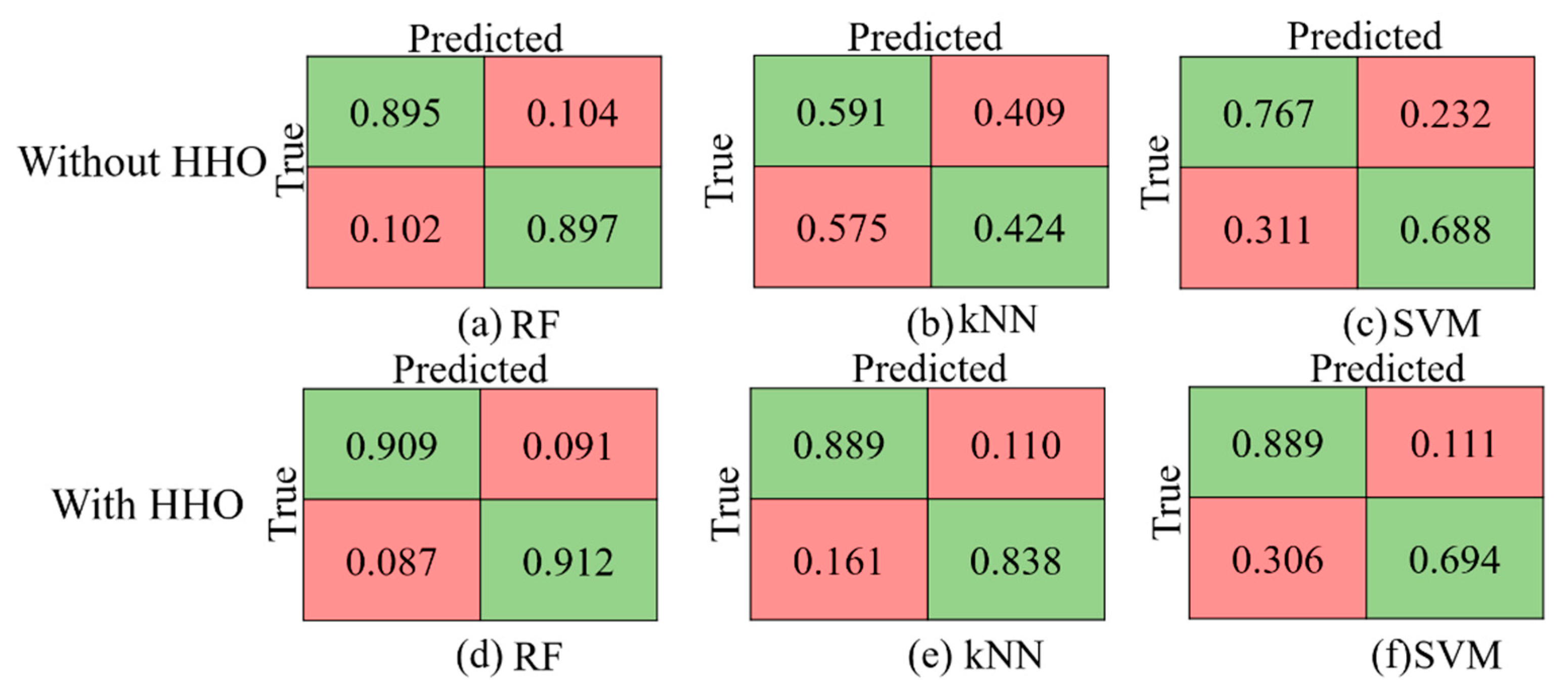
| Method | OA (%) | Precision (%) | MD (%) | FA (%) | F1-Score (%) | BA (%) | Recall (%) | Specificity (%) | KC |
|---|---|---|---|---|---|---|---|---|---|
| RF-HHO | 91.02 | 90.73 | 9.21 | 8.74 | 90.75 | 91.01 | 90.78 | 91.25 | 0.820 |
| RF | 89.65 | 89.17 | 10.43 | 10.26 | 89.36 | 89.65 | 89.56 | 89.73 | 0.793 |
| SVM-HHO | 78.87 | 73.28 | 11.08 | 30.62 | 80.35 | 79.14 | 88.92 | 69.37 | 0.579 |
| SVM | 72.67 | 69.94 | 23.26 | 31.15 | 73.18 | 72.78 | 76.73 | 68.84 | 0.454 |
| kNN-HHO | 86.34 | 83.88 | 11.04 | 16.13 | 86.34 | 86.41 | 88.95 | 83.86 | 0.727 |
| kNN | 58.13 | 56.80 | 40.89 | 42.43 | 57.92 | 58.33 | 59.10 | 57.56 | 0.166 |
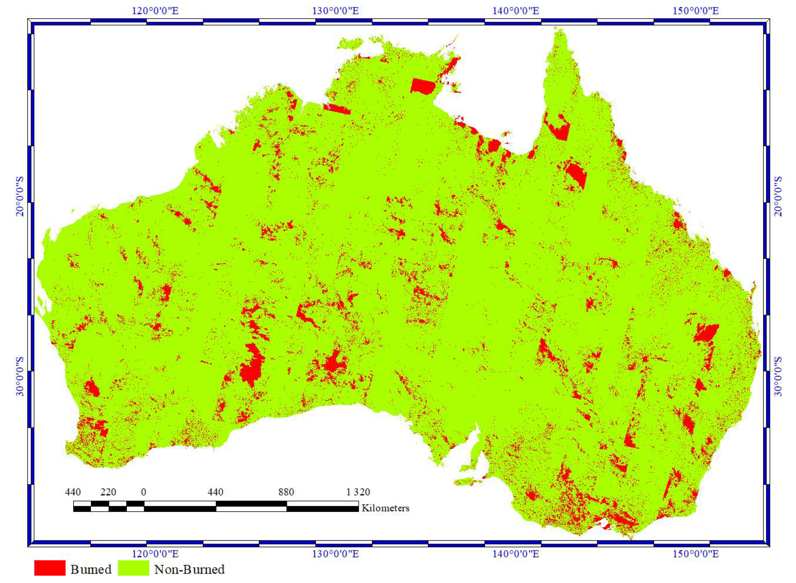
| Class | Area (km2) | Burned Percentage of Individual Class (%) |
|---|---|---|
| Evergreen Needleleaf Forests | 5629 | 25 |
| Evergreen Broadleaf Forests | 27,360 | 24 |
| Deciduous Needleleaf Forests | 0 | 0 |
| Deciduous Broadleaf Forests | 101 | 12 |
| Mixed Forests | 203 | 6 |
| Closed Shrublands | 11,160 | 6 |
| Open Shrublands | 71,511 | 5 |
| Woody Savannas | 8872 | 11 |
| Savannas | 27,878 | 9 |
| Grasslands | 91,106 | 1 |
| Permanent Wetlands | 393 | 8 |
| Croplands | 5034 | 5 |
| Urban and Built-up Lands | 87 | 2 |
| Cropland/Natural Vegetation Mosaics | 24 | 7 |
| Permanent Snow and Ice | 0 | 0 |
| Barren | 0 | 0 |
| Water Bodies | 0 | 0 |
| Total Area = 249,358 (km2) | ||
Publisher’s Note: MDPI stays neutral with regard to jurisdictional claims in published maps and institutional affiliations. |
© 2021 by the authors. Licensee MDPI, Basel, Switzerland. This article is an open access article distributed under the terms and conditions of the Creative Commons Attribution (CC BY) license (http://creativecommons.org/licenses/by/4.0/).
Share and Cite
Seydi, S.T.; Akhoondzadeh, M.; Amani, M.; Mahdavi, S. Wildfire Damage Assessment over Australia Using Sentinel-2 Imagery and MODIS Land Cover Product within the Google Earth Engine Cloud Platform. Remote Sens. 2021, 13, 220. https://0-doi-org.brum.beds.ac.uk/10.3390/rs13020220
Seydi ST, Akhoondzadeh M, Amani M, Mahdavi S. Wildfire Damage Assessment over Australia Using Sentinel-2 Imagery and MODIS Land Cover Product within the Google Earth Engine Cloud Platform. Remote Sensing. 2021; 13(2):220. https://0-doi-org.brum.beds.ac.uk/10.3390/rs13020220
Chicago/Turabian StyleSeydi, Seyd Teymoor, Mehdi Akhoondzadeh, Meisam Amani, and Sahel Mahdavi. 2021. "Wildfire Damage Assessment over Australia Using Sentinel-2 Imagery and MODIS Land Cover Product within the Google Earth Engine Cloud Platform" Remote Sensing 13, no. 2: 220. https://0-doi-org.brum.beds.ac.uk/10.3390/rs13020220