Roll Calibration for CryoSat-2: A Comprehensive Approach
by
 , , , and
Albert Garcia-Mondéjar
1,* ,
,
Michele Scagliola
2 ,
,
Noel Gourmelen
3,4,
Jerome Bouffard
5 and
Mònica Roca
1 1
isardSAT S.L., Barcelona Advanced Industry Park, 08042 Barcelona, Spain
2
Aresys SRL, 20132 Milano, Italy
3
School of GeoSciences, University of Edinburgh, Drummond Street, Edinburgh EH8 9XP, UK
4
IPGS UMR 7516, Université de Strasbourg, CNRS, 67000 Strasbourg, France
5
ESA ESRIN, 00044 Frascati, Italy
*
Author to whom correspondence should be addressed.
Remote Sens. 2021, 13(2), 302; https://0-doi-org.brum.beds.ac.uk/10.3390/rs13020302
Submission received: 29 November 2020
/
Revised: 3 January 2021
/
Accepted: 5 January 2021
/
Published: 16 January 2021
(This article belongs to the Section Ocean Remote Sensing)
Abstract
:CryoSat-2 is the first satellite mission carrying a high pulse repetition frequency radar altimeter with interferometric capability on board. Across track interferometry allows the angle to the point of closest approach to be determined by combining echoes received by two antennas and knowledge of their orientation. Accurate information of the platform mispointing angles, in particular of the roll, is crucial to determine the angle of arrival in the across-track direction with sufficient accuracy. As a consequence, different methods were designed in the CryoSat-2 calibration plan in order to estimate interferometer performance along with the mission and to assess the roll’s contribution to the accuracy of the angle of arrival. In this paper, we present the comprehensive approach used in the CryoSat-2 Mission to calibrate the roll mispointing angle, combining analysis from external calibration of both man-made targets, i.e., transponder and natural targets. The roll calibration approach for CryoSat-2 is proven to guarantee that the interferometric measurements are exceeding the expected performance.
1. Introduction
The CryoSat-2 mission was designed to measure changes in the thickness of sea and land ice fields [1]. The requirements of the system were defined in terms of the uncertainty of the perennial ice thickness change measurement caused by all contributing elements, including satellite performance and ground processing capabilities [2]. The altimeter mounted on board the CryoSat-2 satellite, namely SAR/Interferometric Radar Altimeter (SIRAL), was designed with synthetic aperture and interferometry capabilities in order to meet those requirements. It works in three operating modes: Synthetic Aperture mode (SAR), SAR Interferometric mode (SARIn) and Low-Resolution Mode (LRM). SARIn mode enables aperture synthesis, as does SAR mode, but using two antennas for phase comparison (interferometry) between the radar echoes sensed by them allows us to determine the across-track direction of the return echo. Additionally, CryoSat-2 has three Star Trackers in charge of measuring satellite orientation. The quaternions computed from them have inherent biases of ~1μrad. According to [3], the worst case error on the angle of arrival for CryoSat-2 was expected to be 411μrad. Starting from the error budget for the angle of arrival in [3], in the framework of the roll calibration, we can consider the requirement of the roll bias accuracy to be given by the sum of the instrument internal calibration accuracy and of the contribution from uncorrected thermal deformation of the star tracker-bench-antenna assembly, resulting in 176μrad.
However, different studies revealed that the mispointing angles in the early versions of the CryoSat-2 Level1b were affected by static offsets [4,5,6], which are now compensated [7]. Both the roll and pitch biases are related to inaccuracies in the rotations applied to the Star Tracker quaternions to translate them from their internal reference frame to the interferometer baseline one.
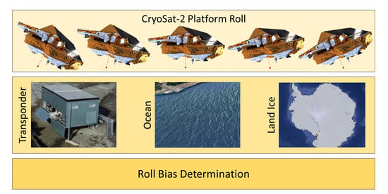
A comprehensive approach has been exploited for the calibration of the roll mispointing due to its direct impact on the accuracy of the across-track angle of arrival (AoA) retrieved by interferometric processing. Three different activities within the CryoSat-2 QWG (Quality Working Group) have been able to analyze the CryoSat-2 roll bias with three different strategies: (i) calibration over the Svalbard transponder [8], (ii) ocean roll campaigns, and (iii) analysis of CryoSat-2 swath data over land ice.
Transponder acquisitions have been used to monitor range, datation, and interferometric phase performances since the beginning of the CryoSat-2 mission. The transponder tracking is programmed twice a month, and the data is analyzed continuously providing a very useful way to detect not only drifts in the component of the instrument but also anomalies in the on-board and ground processors. Calibration campaigns have been periodically performed in order to monitor CryoSat-2 interferometer performances. The calibration strategy for the interferometer uses the open ocean as a well-known target. It is characterized by a rough uniform sloped surface. CryoSat-2 SARIn acquisitions are used to measure the slope of the surface in the across-track direction. They are compared with the a priori known slope of the ocean surface.
Analysis of the interferometric measurements from the calibration campaigns revealed that (i) the roll angle measured by the Star Trackers has a bias with respect to the measured angle of arrival, (ii) this roll bias depends on the Star Tracker being used, and (iii) the accuracy of the roll can be improved by properly correcting the mispointing angles for the aberration of light [9]. The swath processing method was not foreseen to be used for calibration purposes. Although the method was initially used with the CryoSat-2 proof of concept airborne campaigns, it was applied to CryoSat-2 data for the first time 5 years after it was launched.
By analyzing the capabilities of the three methods, the following considerations can be drawn. With the ocean roll campaigns, better precision is achieved, and errors linked to the baseline orientation knowledge can be ignored. However, it has the drawback of requiring spacecraft maneuvers, causing the suspension of science acquisitions. On the other hand, transponder calibration has the great advantage of being very frequent and can perform absolute calibration measurements with just a single pass, which can be also used to detect anomalies. However, it requires a transponder site facility, with maintenance over time. Finally, the swath processing method has the advantage of using science acquisitions available over large areas for assessing the roll bias, but a large amount of data over different regions and seasons is required.
2. Methods
2.1. Transponder Calibration
The transponder equipment used for the CryoSat-2 external calibration is located in the Svalbard archipelago. It was designed and installed in 1987, built for ERS-1 usage and refurbished for the CryoSat-2 mission.
The input data for this calibration analysis are the stack breakpoint products over the transponder location that are produced on request by the on-ground Level1 processor. These products include the individual Doppler beams that have been steered exactly to the Transponder location, providing a very good alignment and signal-to-noise ratio. With these I&Q (in-phase and quadrature signal components) focused beams, the power and phase from both receiving chains can be extracted. The phase difference (Φ (t,r)) is a vector of 1024 range bins (after a zero padding of 2) with the difference between the phase of the signal received from both chains. The angle of arrival measured by the instrument is obtained from the retracked (ri) phase difference (a single value from the 1024 is selected) with
where is the wavelength of the radar signal, 22.084 mm; B is the distance between the centres of two antennas, 1.1676 m; is the roll angle; and Φ (t,r) is the measured phase difference in radians, varying for every beam (t).
The theoretical angle of arrival is computed by geometry (as shown in Figure 1) following:
where d0 is the distance from the closest point of the ground track to the transponder position, r(t) is the distance from the transponder location to the satellite burst locations, and is the across track angle (angle between line from the satellite to the transponder position and the nadir direction).
Finally, the bias is computed as the difference between the measured and the theoretical angle of arrivals.
2.2. Roll Campaigns over Ocean
The operational calibration plan for CryoSat-2 foresees that interferometer calibration campaigns are periodically performed for calibration purposes, complementing the acquisitions over transponder. An interferometer calibration campaign consists of a sequence of SIRAL acquisitions in SARIn mode over the tropical and mid latitude oceans while the spacecraft is rolling from side to side at about ±0.4 degrees. The range of commanded roll angles was defined to be representative of the range of slopes that are expected to be experienced while acquiring over ice sheets.
During interferometer calibration campaigns, the purpose of the CryoSat-2 interferometer is to estimate the across-track slope of the ocean surface [4], so that the end-to-end error on the angle of arrival is assessed by comparison of the measured across-track slope with an a-priori known across-track slope. The acquisition geometry is represented in Figure 2. We denote the roll angle as , the across-track slope of the ocean surface as β and the angle made by the direction of first arrival (i.e., Point of Closest Approach, POCA) with antennas′ boresight direction as . It is worth recalling that the interferometer baseline is defined as the vector following the direction between antenna 1 (the transmitting/receiving antenna, left one in Figure 2) and antenna 2 phase centers (the receiving only antenna, right one in Figure 2). Since the interferometer baseline is kept in flight orthogonal to the ground track, the orientation of the interferometer baseline in the across-track plane corresponds to the roll angle . According to the acquisition geometry in Figure 2, the across-track slope of the ocean surface results in
where is a geometric factor that is given by being h, the altitude of the satellite with respect to the ellipsoid, and R is the Earth′s radius.
Recalling that the angle of first arrival in the across-track plane can be computed by evaluating the interferometric phase difference at POCA, Φ0, we found that the end-to-end error on the AoA resulted in
where is the carrier wavenumber and is the interferometer baseline length. According to the definition above, the end-to-end error is composed of three different terms: (i) the error contribution from the measured angle of arrival , which includes the SIRAL instrument noise and inaccuracies from the Level1 ground processor and interferometer calibration tool; (ii) the knowledge error on roll , which is given by the combination of the internal accuracy of Star Trackers and ground processing of downlinked quaternions; and (iii) the knowledge error on the a-priori known ocean surface slope .
According to the considerations drawn in [4], the knowledge error on the ocean surface slope is assumed to be negligibly small, while the error contribution from the measured angle of arrival results in unbiased noise. As a consequence, the end-to-end error on the AoA can be modeled as a linear function of the angle of arrival itself, and the calibration function for the CryoSat-2 interferometer finally results in
where the linear coefficient corresponds to the contribution from the phase departure [1], while the constant term is addressed to a static bias affecting the roll mispointing angle (i.e., a roll bias).
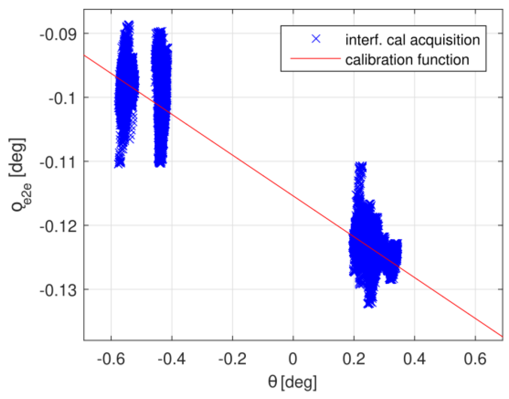
From an operative point of view, the inputs of the interferometer calibration tool are the Level 1b products for the acquisitions commanded during campaigns for the calibration of the CryoSat-2 interferometer. The 20 Hz power waveform is retracked to identify the POCA, and the angle of arrival is computed. Then, according to Equation (5), the error in the angle of arrival is obtained by knowledge of the roll mispointing angle and the ocean surface slope from the geoid. Finally, the parameters for the calibration function for the CryoSat-2 interferometer are obtained by linear regression, as depicted in Figure 3, where the end-to-end error in the angle of arrival for calibration campaign #3 as a function of the angle of arrival and the corresponding calibration function are depicted.
2.3. Swath-Based Roll
When in SARIn mode and in the presence of a suitable across-track angle, namely, typical conditions over land ice, elevation can be retrieved beyond the point-of-closest-approach (POCA), leading to a swath of elevation in the across-track direction [10,11,12]. This approach has been used to improve the spatial resolution of time-dependent elevation change across the two polar ice sheets [12,13,14,15], as well as icecaps and glaciers worldwide [16,17,18,19].
The across-track position and elevation are directly related to the roll angle and the look angle via (2). The existence of a roll bias will lead to an elevation bias between ascending and descending passes; a bias that, within a given waveform, will increase with the distance to the POCA. This elevation bias can then be used to invert the most-likely roll bias by adding a roll bias term to Equation (5) and solving for the roll bias, minimizing the difference in elevation between ascending and descending passes over a common location [12,20]. The approach has so far been implemented by subtracting a reference elevation (e.g., ground-based GPS, operation ice bridge airborne laser altimeter, ASIRAS airborne Ku-band radar altimeter) from the CryoSat-2 data and analyzing the ascending-descending elevation bias to compare the differences in elevation residuals [12,20]. This strategy limits the use of the approach to areas where collocated elevation reference campaigns have been conducted. An alternative, not used here, would be to compare swath crossovers, thus making the approach independent of the use of an accurate reference elevation.
The experiment, then, consists of running the swath processing a number of times with different values of the roll bias; in this instance, we run the experiment with increments of roll bias of 0.01°, and the discrete record is then oversampled to improve the resolution of the roll angle determination. The most likely roll bias is then determined from the width of the elevation residual distribution.
3. Results and Discussion
The results in the following were obtained comparing CryoSat-2 Level1b products from different Baselines, i.e., versions of the products generated by different versions of the Level1 processor and corresponding configuration. Limiting to the mispointing angle computation and the roll bias applied by configuration, the differences between the Baselines are listed in the following: (i) in Baseline-B, the SARIn phase difference was compensated for a 0.1054 degrees roll bias; (ii) in Baseline-C, a roll bias equal to 0.1062 degrees was compensated, and the mispointing angles were computed from the optimal Star Tracker according to an on-board selection; and (iii) in Baseline-D, the roll was compensated for a bias varying as a function of both the Mission lifetime and the Star Tracker in use, while the mispointing angles computation accounted for the aberration of light [7,9].
3.1. Transponder Calibration
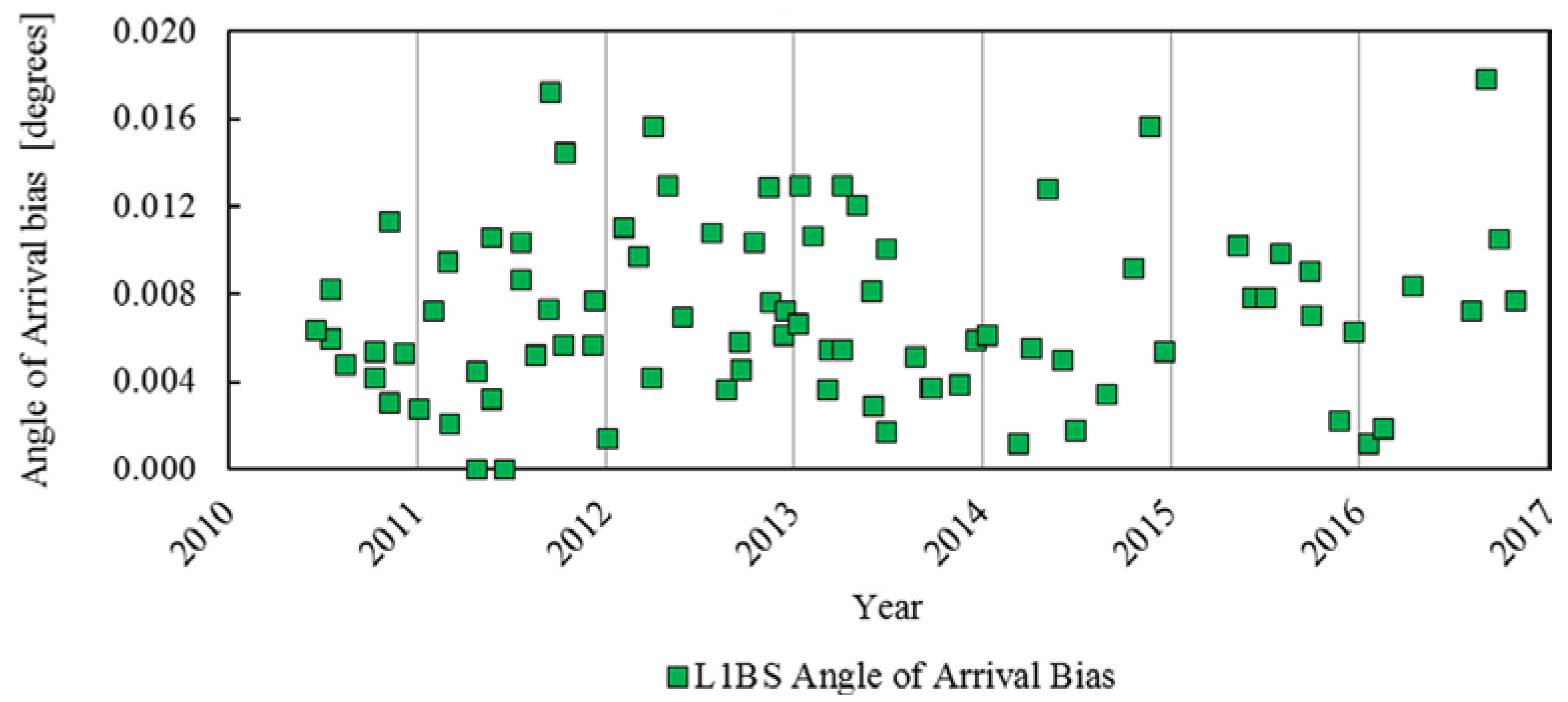
Results for the Angle of Arrival for each Transponder pass are shown in Figure 4. The overall 0.0071 degrees of bias is equivalent to a displacement in the geolocations across-track of about 87 m, and the standard deviation of 0.0040 degrees denotes an uncertainty of around 50 m. The results are slightly within the 0.0083 degrees of AoA requirement.
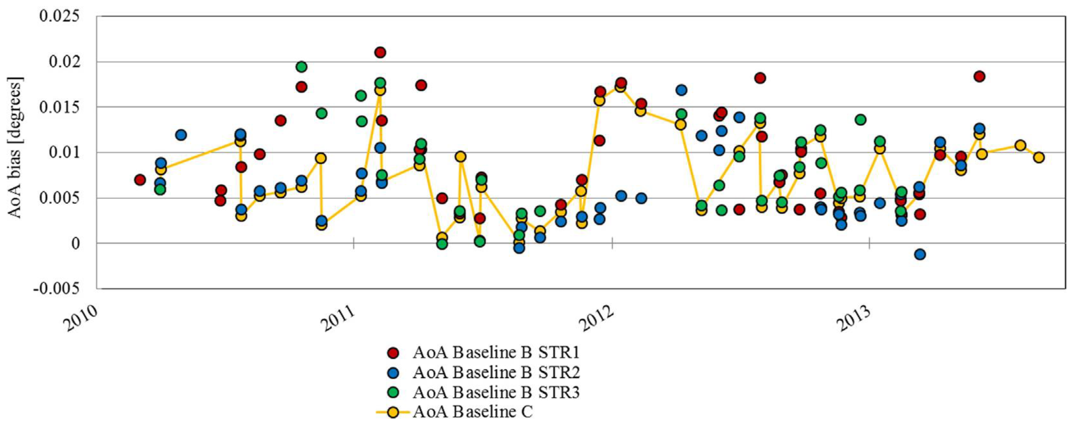
By averaging all the different errors, the AoA bias is 0.0071 degrees, bearing in mind that for each pass, different Star Trackers (STRs) with different temperature conditions have been used. The AoA pass-to-pass results variations depend mainly on the error of the estimation of the roll and are different for each STR, even if they should measure the same. So, for a single transponder pass, different AoA results can be obtained depending on which STR is used to retrieve the attitude. In the Baseline-C processor, a specific module, called an STR processor, is in charge of estimating the attitude [9]. The STR selection method was improved from Baseline-B. The previous method just selected the first available STR, while in Baseline-C, the selected STR is the one used by the Attitude and Orbital Control Systems. Additionally, the STR processor performs smoothing on the roll, pitch and yaw before writing them on the product. Although these changes improve the attitude measurements, the STR selection on board sometimes does not use the STR with the smallest error. A comparison between the AoA results from both baselines is shown in Figure 5. It can be seen that some Baseline-C results are worse than the ones available from Baseline-B. Further studies concluded with the need to implement an improved attitude solution in the Star Tracker processor (currently operational in Baseline-D products).
The links between the AoA results have tried to be related to the temperature of the spacecraft, but the sparse number of transponder passes made analysis difficult. The bending of the antenna bench due to spacecraft interface temperature can cause mispointing from the STRs nominal positions and consequent bias in the attitude measurements. These biases can be corrected by averaging the attitude measured by two opposite STRs, but only in the case where bending is symmetric. However, different illuminations of the sun can increase the attitude noise, making the ‘‘hot” STRs less precise.
3.2. Roll Campaigns over Ocean
Throughout this section, the results of the interferometer calibration analysis of the CryoSat-2 SARIn L1b products from the interferometer calibration campaigns are presented. Table 1 includes the main information for each interferometer calibration campaign.
It is worth recalling that the Star Trackers were placed on the spacecraft to have a different orientation, so that at any time at least one Star Tracker was free from sun or moon blinding (tagged “OFF” on the Table) [2]. This can be verified by inspection of Table 1, where, for each campaign, at least two Star Trackers were available (tagged “ON” on the Table).
The SARIn L1b product only contains mispointing angles computed from the optimal Star Tracker according to the rule defined on board in the attitude orbit control system. In order to include the roll mispointing angle from the Star Tracker available in the calibration analysis, we processed our own the quaternions generated by the Star Trackers using exactly the same processing functions and configuration that are used in Level1 operational processor. This way, a calibration function for each available Star Tracker was computed. It has to be remarked that in the following we present the results of the interferometer calibration obtained (i) by computing the mispointing angles on-ground by properly correcting for the aberration of light [1] and (ii) by exploiting an improved version of the interferometer calibration tool, where the accuracy of the a-priori known across-track ocean slope was increased.
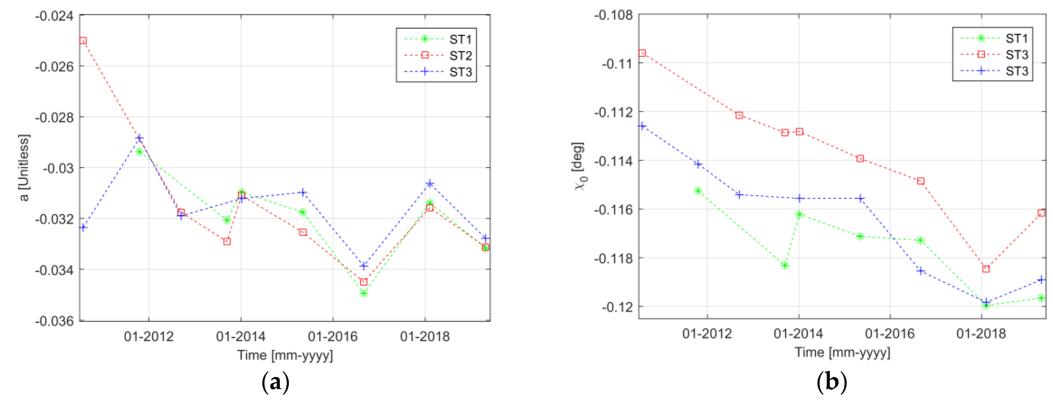
In Figure 6, we plotted the calibration function parameters that were obtained for the different interferometer calibration campaigns and for each available Star Tracker by processing Baseline-C L1b products. By inspection of Figure 6a, where the linear coefficient for the interferometer calibration function is reported, it can be noticed that similar values are obtained from the available Star Trackers for each campaign. This behavior was expected since the parameter a is a function of sea surface roughness only. By inspection of Figure 6b, where the estimated roll bias is reported, it can be noticed that exhibits a dependence on the Star Tracker. This suggests that a different roll bias is present depending on the rotation between each Star Tracker frame and the interferometer baseline. Additionally, a decreasing trend can be observed, at least up to 2018.
It has to be remarked that in Figure 6b the total uncorrected roll bias is presented. Recalling that a roll bias equal to 0.1062 degrees was compensated in Baseline-C, an average residual roll bias of 0.0097 degrees with a standard deviation of 0.0019 degrees is finally obtained. It is worth noticing that the average residual roll bias in Baseline-C was already compliant with the requirement for the roll bias given in Section 1.
As an outcome of the roll calibration exploiting the interferometer calibration campaign over ocean, we decided to apply a different roll bias as function of the Star Tracker and variable as a function of the mission lifetime for the reprocessed products in Baseline-D [20]. By processing Baseline-D products from the interferometer calibration campaigns, the residual roll bias for each Star Tracker shown in Figure 7 was obtained. By inspection of Figure 7, it can be noticed that the residual roll bias in Baseline-D is steadily around zero, independently of the Star Tracker and of the campaign, resulting in an average roll bias of 0.0006 degrees with a standard deviation of 0.0009 degrees.
In the framework of this analysis, the roll bias was subsequently addressed, and the existence of an antenna bench bending for SIRAL was investigated together with its impact on interferometric acquisitions. As detailed in [2], the rigid bench where antennas are mounted is expected to undergo convex or concave flexing when subject to a thermal gradient. To minimize the effect of this bending, antenna feeds are decoupled from the antenna bench while the Star Trackers are coupled with the antenna bench. As a consequence, a bending of the antenna bench can affect the roll measured by the Star Trackers so that the measured roll does not correspond to the real direction of the interferometer antenna baseline. Aiming to evaluate the in-flight flexing of the bench, the difference of the roll measured by each Star Tracker pair was computed. If a difference far from zero is observed for two Star Trackers on opposite sides of the bench, it can be due to its bending, under the assumption of the exact roll computed by Star Trackers and by on-ground processing.
In Figure 8 shows the roll difference for each Star Tracker pair from the beginning of the mission up to 2017. It can be noticed that roll differences between Star Trackers on the same side of the antenna bench are nearly zero, as expected. On the other hand, the roll differences between Star Trackers on the opposite side of the antenna bench is larger than zero in absolute value and varies as a function of mission lifetime.
Under the assumption that the roll difference of Star Tracker pairs at different sides of the antenna bench is due to bending and that the bending is symmetrical with respect to the center of the antenna bench, the error in the angle of arrival due to bench bending can be modeled as equal to half the roll difference. Considering the whole mission, the average error in the angle on arrival due to bench bending at 1Hz is equal to 0.0020 degrees with a standard deviation equal to 0.0112 degrees.
3.3. Swath-Based Roll
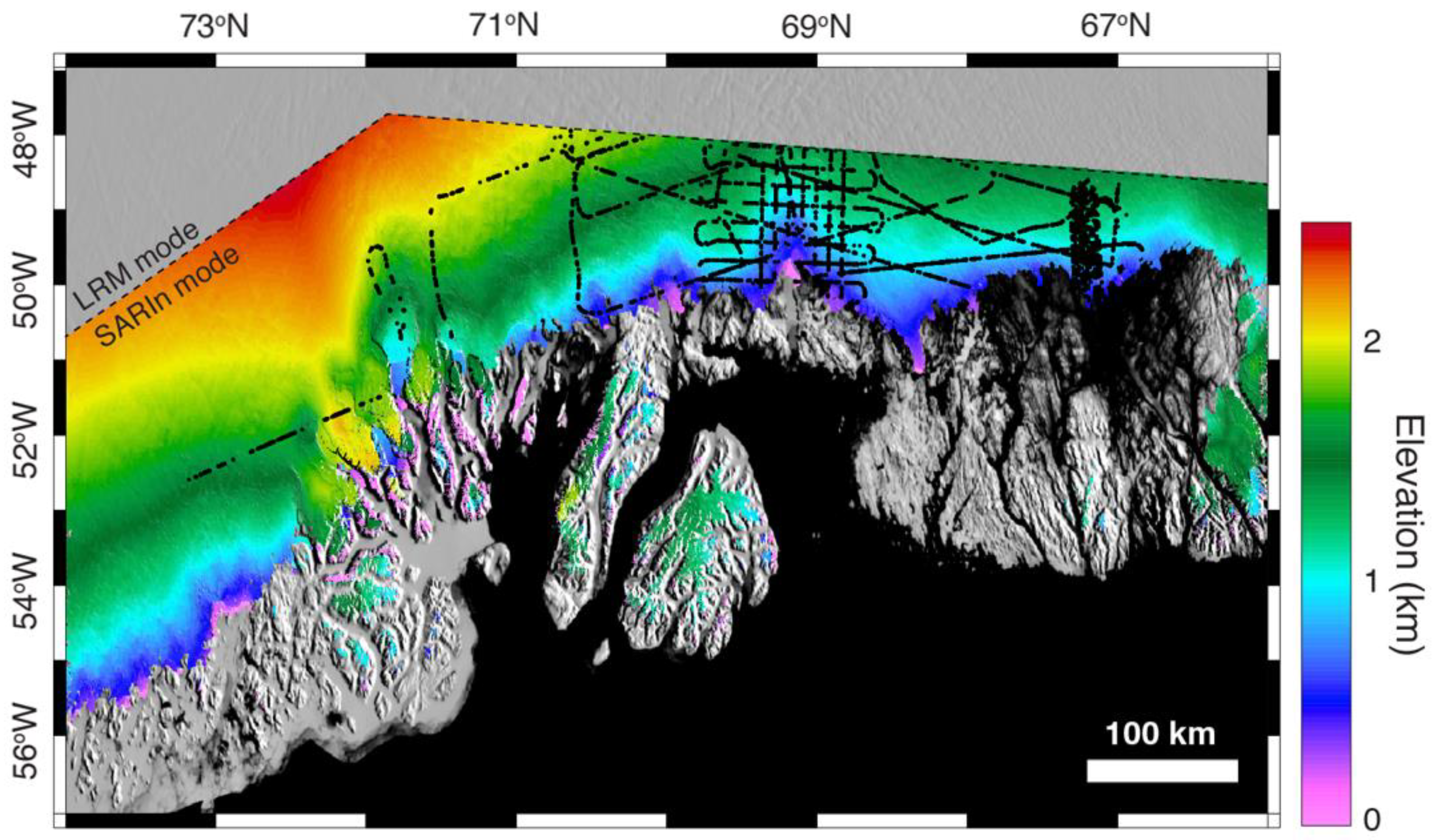
This approach has been applied over the Greenland Ice Sheet, where OIB (Operation Ice Bridge) [21] surveys have been conducted yearly during the CryoSat-2 period (Figure 9). To limit the chance of elevation difference occurring due to temporal change and surface slopes, each CryoSat-2 height record has been matched with the closest OIB elevation, setting a maximum spatial distance of 50 m and temporal separation of 10 days. The elevation difference between OIB and CryoSat-2 due to their different positions is further corrected using arcticDEM [22] as reference topography.
From the CryoSat-2 and the OIB datasets covering the month of April 2011, we obtained over 50,000 collocated measurements equally split between ascending and descending orbits.
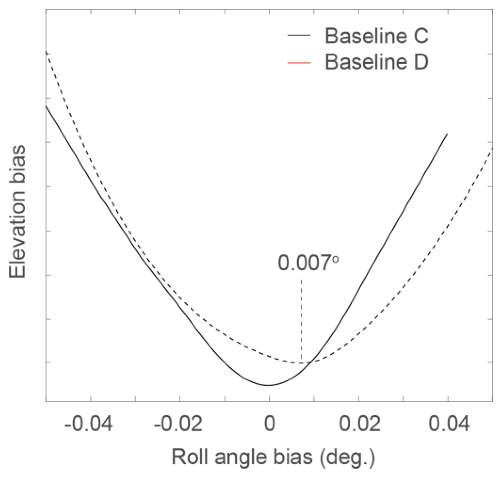
Analysis of the Baseline-C dataset reveals a clear minimum elevation bias found for a roll bias of ~0.007°, a value in agreement with the alternative methods described alongside the swath method, as seen in Figure 10. The same analysis of Baseline-D data again shows a clear minimum, but this time it is centered on ~0°, an expected outcome since Baseline-D data incorporate the improved attitude. We also note that the width of the minimization is reduced for Baseline-D case compared with Baseline-C, suggesting that the attitude correction performed on Baseline-D data has addressed some of the variability in the roll error seen in Baseline-C data.
The chosen strategy of using a reference elevation, in this case, OIB airborne laser, limits the use of this approach to areas where collocated elevation reference campaigns have been conducted. An alternative approach would be to extract point-to-point elevation difference from ascending and descending passes. This latter approach would allow us to exploit more of the CryoSat-2 datasets and analyze the roll bias as a function of orbit position and time to assess external forcings in the roll-bias variation.
This approach could also lead to continuous platform attitude assessment and correction as no particular campaign needs to be programmed. This would potentially reduce some of the largest errors related to uncertainty in the Angle of Arrival and subsequent errors in geophysical variables extracted from Interferometric Radar Altimeters.
4. Conclusions
Three different methods have been used to determine roll stability during the CryoSat-2 mission. Analysis with transponder acquisitions provided a very accurate and uniform solution thanks to the good knowledge of the target and the frequency of the acquisitions (twice a month uninterruptedly). However, it was difficult to measure seasonal distortions related to the bench bending and to disregard an error due to phase difference from errors due to antenna baseline orientation knowledge. Analysis of the roll campaign data over ocean increased the number of records analyzed compared with single target measurements over the transponders. However, the complexity of the roll campaign only allowed for 9 campaigns, compared with the 87 transponder passes. The swath method provided a very good approach, with the ability to use science data directly over a specific land ice region, but it required the use of an additional instrument to measure the reference elevation, which limited the use of the method to areas where collocated elevation reference campaigns had been conducted. Alternatively, swath crossovers could be used, which would not rely on such reference elevation. A comparison of the roll bias results for each of the methods is listed in Table 2 in the case of Baseline-C.
Author Contributions
The contributions of this reported work can be listed as follows: writing-original draft preparation, A.G.-M.; writing—review and editing A.G.-M. Transponder analysis M.R., A.G.-M.; roll campaigns over ocean M.S.; Swath-based analysis N.G.; supervision and final revision M.R., J.B. All authors have read and agreed to the published version of the manuscript.
Funding
This work has been developed in the framework of ESA/ESTEC (Contracts No. C18318/05/NL and 4200022114/08/NL/JA), ESA/ESRIN (Contracts No. 4000104810/11/I-NB and 4000111597/14/I-AM and 4000111474/14/I-NB and 4000107394/12/I-NB and 4000116874/16/I-NB).
Data Availability Statement
The input data used in this manuscript can be freely downloaded from ESA portal. Transponder and Land Ice data from the CryoSat-2 Science Server (https://science-pds.cryosat.esa.int/) and the roll campaigns from its specific portal (https://earth.esa.int/web/guest/missions/esa-eo-missions/cryosat/roll-campaigns).
Acknowledgments
We would like to thank the participants of the ESA CryoSat-2 Quality Working Group for the interesting exchanges and discussions.
Conflicts of Interest
The authors declare no conflict of interest.
References
- Wingham, D.J.; Phalippou, L.; Mavrocordatos, C.; Wallis, D. The mean echo and echo cross product from a beamforming interferometric altimeter and their application to elevation measurement. IEEE Trans. Geosci. Rem. Sens. 2004, 42, 2305–2323. [Google Scholar] [CrossRef]
- ESA Team. CryoSat Mission and Data Description; Report no. CS-RP-ESA-SY-0059; ESTEC: Noordwijk, The Netherlands, 2007; Available online: http://esamultimedia.esa.int/docs/Cryosat/Mission_and_Data_Descrip.pdf (accessed on 15 January 2021).
- Wingham, D.J.; Francis, C.R.; Baker, S.; Bouzinac, C.; Brockley, D.; Cullen, R.; de Chateau-Thierry, P.; Laxon, S.W.; Mallow, U.; Mavrocordatos, C.; et al. CryoSat: A mission to determine the fluctuations in Earth’s land and marine ice fields. Adv. Space Res. 2006, 37, 841–871. [Google Scholar] [CrossRef]
- Galin, N.; Wingham, D.J.; Cullen, R.; Fornari, M.; Smith, W.H.F.; Abdalla, S. Calibration of the CryoSat-2 Interferometer and Measurement of Across-Track Ocean Slope. IEEE Trans. Geosci. Remote Sens. 2012, 51, 57–72. [Google Scholar] [CrossRef]
- Galin, N.; Wingham, D.J.; Cullen, R.; Francis, R.; Lawrence, I. Measuring the Pitch of CryoSat-2 Using the SAR Mode of the SIRAL Altimeter. IEEE Geosci. Remote Sens. Lett. 2014, 11, 1399–1403. [Google Scholar] [CrossRef]
- Scagliola, M.; Fornari, M.; Tagliani, N. Pitch Estimation for CryoSat by Analysis of Stacks of Single-Look Echoes. IEEE Geosci. Remote Sens. Lett. 2015, 12, 1561–1565. [Google Scholar] [CrossRef]
- Meloni, M.; Bouffard, J.; Parrinello, T.; Dawson, G.; Garnier, F.; Helm, V.; Di Bella, A.; Hendricks, S.; Ricker, R.; Webb, E.; et al. CryoSat Ice Baseline-D validation and evolutions. Cryosphere 2020, 14, 1889–1907. [Google Scholar] [CrossRef]
- Garcia-Mondéjar, A.; Fornari, M.; Bouffard, J.; Féménias, P.; Roca, M. CryoSat-2 range, datation and interferometer calibration with Svalbard transponder. Adv. Space Res. 2018, 62, 1589–1609. [Google Scholar] [CrossRef]
- Scagliola, M.; Fornari, M.; Bouffard, J.; Parrinello, T. The CryoSat interferometer: End-to-end calibration and achievable performance. Adv. Space Res. 2018, 62, 1516–1525. [Google Scholar] [CrossRef]
- Hawley, R.L.; Shepherd, A.; Cullen, R.; Helm, V.; Wingham, D.J. Ice-sheet elevations from across-track processing of airborne interferometric radar altimetry. Geophys. Res. Lett. 2009, 36, L22501. [Google Scholar] [CrossRef] [Green Version]
- Gray, L.; Burgess, D.; Copland, L.; Cullen, R.; Galin, N.; Hawley, R.; Helm, V. Interferometric swath processing of Cryosat-2 data for glacial ice topography. Cryosphere Discuss. 2013, 7, 3133–3162. [Google Scholar] [CrossRef]
- Gourmelen, N.; Escorihuela, M.J.; Shepherd, A.; Foresta, L.; Muir, A.; Garcia-Mondejar, A.; Drinkwater, M.R. CryoSat-2 swath interferometric altimetry for mapping ice elevation and elevation change. Adv. Space Res. 2018, 62, 1226–1242. [Google Scholar] [CrossRef] [Green Version]
- Gourmelen, N.; Goldberg, D.; Snow, K.; Henley, S.; Bingham, R.; Kimura, S.; Hogg, A.; Shepherd, A.; Mouginot, J.; Lenearts, J.; et al. Channelized melting drives thinning under a rapidly melting Antarctic ice shelf. Geophys. Res. Lett. 2017, 44, 9796–9804. [Google Scholar] [CrossRef]
- Gray, L.; Burgess, D.; Copland, L.; Langley, K.; Gogineni, P.; Paden, J.; Smith, B. Measuring height change around the periphery of the Greenland Ice Sheet with radar altimetry. Front. Earth Sci. 2019, 7, 146. [Google Scholar] [CrossRef]
- Shepherd, A.; Ivins, E.; Rignot, E.; Smith, B.; van Den Broeke, M.; Velicogna, I.; Whitehouse, P.; Briggs, K.; Joughin, I.; Krinner, G.; et al. Mass balance of the Greenland Ice Sheet from 1992 to 2018. Nature 2020, 579, 233–239. [Google Scholar]
- Gray, L.; Burgess, D.; Copland, L.; Demuth, M.N.; Dunse, T.; Langley, K.; Schuler, T.V. CryoSat-2 delivers monthly and inter-annual surface elevation change for Arctic ice caps. Cryosphere 2015, 9, 1895–1913. [Google Scholar] [CrossRef] [Green Version]
- Foresta, L.; Gourmelen, N.; Pálsson, F.; Nienow, P.; Björnsson, H.; Shepherd, A. Surface elevation change and mass balance of Icelandic ice caps derived from swath mode CryoSat-2 altimetry. Geophys. Res. Lett. 2016, 43, 12138–12145. [Google Scholar] [CrossRef] [Green Version]
- Foresta, L.; Gourmelen, N.; Weissgerber, F.; Nienow, P.; Williams, J.; Shepherd, A.; Drinkwater, M.R.; Plummer, S. Heterogeneous and rapid ice loss over the Patagonian Ice Fields revealed by CryoSat-2 swath radar altimetry. Remote Sens. Environ. 2018, 211, 441–455. [Google Scholar] [CrossRef]
- Jakob, L.; Gourmelen, N.; Ewart, M.; Plummer, S. Ice loss in High Mountain Asia and the Gulf of Alaska observed by CryoSat-2 swath altimetry between 2010 and 2019. Cryosphere 2020. [Google Scholar] [CrossRef]
- Gray, L.; Burgess, D.; Copland, L.; Dunse, T.; Langley, K.; Moholdt, G. A revised calibration of the interferometric mode of the CryoSat-2 radar altimeter improves ice height and height change measurements in western Greenland. Cryosphere 2017, 11, 1041–1058. [Google Scholar] [CrossRef] [Green Version]
- Studinger, M.; Koenig, L.; Martin, S.; Sonntag, J. Operation icebridge: Using instrumented aircraft to bridge the observational gap between Icesat and Icesat-2. IEEE Inter. Geosci. Remote Sens. Symp. 2010. [Google Scholar] [CrossRef]
- Morin, P.; Porter, C.; Cloutier, M.; Howat, I.; Noh, M.J.; Willis, M.; Bates, B.; Williamson, C.; Peterman, K. ArcticDEM; A publically available, high resolution elevation model of the Arctic. In Proceedings of the EGUGA 2016, Vienna, Austria, 17–22 April 2016. EPSC2016-8396. [Google Scholar]
- Haran, T.; Bohlander, J.; Scambos, T.; Fahnestock, M. Modis Mosaic of Greenland (Mog) Image Map; NSIDC—National Snow and Ice Data Center: Boulder, CO, USA, 2013. [Google Scholar]
- Howat, I.M.; Negrete, A.; Smith, B.E. The Greenland Ice Mapping Project (GIMP) land classification and surface elevation data sets. Cryosphere 2014, 8, 1509–1518. [Google Scholar] [CrossRef] [Green Version]
Figure 1.
Geometry of the angle of arrival with transponder (TRP) measurements. CryoSat-2 sends and receives pulses to the transponder location along the overpass. Figure taken from [8].
Figure 1.
Geometry of the angle of arrival with transponder (TRP) measurements. CryoSat-2 sends and receives pulses to the transponder location along the overpass. Figure taken from [8].

Figure 2.
Roll campaigns: acquisition geometry in the across-track plane (angles exaggerated for clarity). β represents the ocean across the track slope and the platform roll angle. Figure taken from [9].
Figure 2.
Roll campaigns: acquisition geometry in the across-track plane (angles exaggerated for clarity). β represents the ocean across the track slope and the platform roll angle. Figure taken from [9].

Figure 3.
End-to-end error in the angle of arrival for calibration campaign #3 as a function of the angle of arrival and the corresponding calibration function. The blue points represent the individual interferometric measurements and the red line the linear regression over them. Figure taken from [9].

Figure 4.
Angle of Arrival (AoA) calibration with transponder results. Each point represents the retrieval for a single transponder pass. Figure taken from [8].
Figure 4.
Angle of Arrival (AoA) calibration with transponder results. Each point represents the retrieval for a single transponder pass. Figure taken from [8].

Figure 5.
Baseline-B and Baseline-C AoA results. Read, blue and green points represent the individual AoA retrievals for Star Trackers (STRs) 1, 2 and 3. Yellow dots represent the retrieval of the STR selected by the STR processor. Figure taken from [8].
Figure 5.
Baseline-B and Baseline-C AoA results. Read, blue and green points represent the individual AoA retrievals for Star Trackers (STRs) 1, 2 and 3. Yellow dots represent the retrieval of the STR selected by the STR processor. Figure taken from [8].

Figure 6.
Calibration function parameters from Baseline-C L1b products: (a) linear coefficient a and (b) constant term .
Figure 6.
Calibration function parameters from Baseline-C L1b products: (a) linear coefficient a and (b) constant term .

Figure 7.
Residual roll bias from Baseline-C and Baseline-D acquisitions.

Figure 8.
Roll difference for each Star Tracker pair. Blue represents differences between ST1 and ST3, yellow between ST2 and ST3, and red between ST1 and ST2.
Figure 8.
Roll difference for each Star Tracker pair. Blue represents differences between ST1 and ST3, yellow between ST2 and ST3, and red between ST1 and ST2.

Figure 9.
Location of the collocated swath-OIB (Operation Ice Bridge) measurements. EOLIS (Elevation Over Land Ice from Swath) DEM along the west coast of the Greenland Ice Sheet overlaid over the MEaSUREs MODIS (Moderate Resolution Imaging Spectroradiometer) Mosaic of Greenland [23]. The inland limit of the DEM corresponds to the CryoSat-2′s SARIn mode mask (dashed line); elsewhere the ice mask is in accordance with the Greenland Ice Mapping Project (GIMP) dataset [24]. Ice Bridge elevation acquired in March, April and May 2011 (black). Figure taken from [12].

Figure 10.
Elevation bias between ascending and descending CryoSat-2 passes as a function of roll angle bias. The roll bias that minimizes the dispersion of the elevation difference for Baseline-C data is found at 0.007°. The same exercise using Baseline-D data shows a minimum elevation dispersion with no significant roll angle bias. Figure taken from [12].


Table 1.
Interferometer calibration campaigns.
| Campaign | Dates | L1b Products | ST1 | ST2 | ST3 |
|---|---|---|---|---|---|
| #1 | 27–28 July 2010 | 6 | OFF | ON | ON |
| #2 | 17–18 October 2011 | 9 | ON | OFF | ON |
| #3 | 11–12 September 2012 | 8 | OFF | ON | ON |
| #4 | 10–12 October 2013 | 8 | ON | ON | OFF |
| #5 | 4–5 January 2014 | 8 | ON | ON | ON |
| #6 | 6 May 2015 | 8 | ON | ON | ON |
| #7 | 31 August–1 September 2016 | 8 | ON | ON | ON |
| #8 | 6 February 2018 | 8 | ON | ON | ON |
| #9 | 25 April 2019 | 8 | ON | ON | ON |
Table 2.
Comparison of the roll bias results for Baseline-C.
| Method | Bias | Standard Deviation |
|---|---|---|
| Transponder | 0.0071 degrees | 0.0040 degrees |
| Ocean Roll | 0.0097 degrees | 0.0019 degrees |
| Swath | 0.0070 degrees | - |
Aiming at taking advantage of the capabilities and advantages of each of the methods, the comprehensive approach for roll calibration that has been exploited in the CryoSat-2 Mission foresees that (i) absolute roll bias is evaluated using the campaign data over ocean; (ii) the stability of the roll mispointing is continuously monitored, exploiting the transponder acquisitions; and (iii) the performance from a user perspective is assessed using swath data analysis. Following the approach above, it was possible to refine the roll bias correction in Baseline-D, and this in turn was proven to reduce the residual roll bias with a direct impact on the quality of interferometric measurements.
Publisher’s Note: MDPI stays neutral with regard to jurisdictional claims in published maps and institutional affiliations. |
© 2021 by the authors. Licensee MDPI, Basel, Switzerland. This article is an open access article distributed under the terms and conditions of the Creative Commons Attribution (CC BY) license (http://creativecommons.org/licenses/by/4.0/).
Share and Cite
MDPI and ACS Style
Garcia-Mondéjar, A.; Scagliola, M.; Gourmelen, N.; Bouffard, J.; Roca, M. Roll Calibration for CryoSat-2: A Comprehensive Approach. Remote Sens. 2021, 13, 302. https://0-doi-org.brum.beds.ac.uk/10.3390/rs13020302
AMA Style
Garcia-Mondéjar A, Scagliola M, Gourmelen N, Bouffard J, Roca M. Roll Calibration for CryoSat-2: A Comprehensive Approach. Remote Sensing. 2021; 13(2):302. https://0-doi-org.brum.beds.ac.uk/10.3390/rs13020302
Chicago/Turabian StyleGarcia-Mondéjar, Albert, Michele Scagliola, Noel Gourmelen, Jerome Bouffard, and Mònica Roca. 2021. "Roll Calibration for CryoSat-2: A Comprehensive Approach" Remote Sensing 13, no. 2: 302. https://0-doi-org.brum.beds.ac.uk/10.3390/rs13020302
Note that from the first issue of 2016, this journal uses article numbers instead of page numbers. See further details here.