Article

Error Correction of Multi-Source Weighted-Ensemble Precipitation (MSWEP) over the Lancang-Mekong River Basin

1
State Key Laboratory of Hydrology-Water Resources and Hydraulic Engineering, Nanjing 210098, China
2
Nanjing Hydraulic Research Institute, Nanjing 210029, China
3
Research Center for Climate Change, Ministry of Water Resources, Nanjing 210029, China
*
Author to whom correspondence should be addressed.
Submission received: 18 December 2020 / Revised: 12 January 2021 / Accepted: 15 January 2021 / Published: 18 January 2021
(This article belongs to the Special Issue Remote Sensing in Hydrology and Water Resources Management)

Abstract

:
The demand for accurate long-term precipitation data is increasing, especially in the Lancang-Mekong River Basin (LMRB), where ground-based data are mostly unavailable and inaccessible in a timely manner. Remote sensing and reanalysis quantitative precipitation products provide unprecedented observations to support water-related research, but these products are inevitably subject to errors. In this study, we propose a novel error correction framework that combines products from various institutions. The NASA Modern-Era Retrospective Analysis for Research and Applications (AgMERRA), the Asian Precipitation Highly-Resolved Observational Data Integration Towards Evaluation of Water Resources (APHRODITE), the Climate Hazards group InfraRed Precipitation with Stations (CHIRPS), the Multi-Source Weighted-Ensemble Precipitation Version 1.0 (MSWEP), and the Precipitation Estimation from Remotely Sensed Information using Artificial Neural Networks-Climate Data Records (PERSIANN) were used. Ground-based precipitation data from 1998 to 2007 were used to select precipitation products for correction, and the remaining 1979–1997 and 2008–2014 observe data were used for validation. The resulting precipitation products MSWEP-QM derived from quantile mapping (QM) and MSWEP-LS derived from linear scaling (LS) are evaluated by statistical indicators and hydrological simulation across the LMRB. Results show that the MSWEP-QM and MSWEP-LS can better capture major annual precipitation centers, have excellent simulation results, and reduce the mean BIAS and mean absolute BIAS at most gauges across the LMRB. The two corrected products presented in this study constitute improved climatological precipitation data sources, both time and space, outperforming the five raw gridded precipitation products. Among the two corrected products, in terms of mean BIAS, MSWEP-LS was slightly better than MSWEP-QM at grid-scale, point scale, and regional scale, and it also had better simulation results at all stations except Strung Treng. During the validation period, the average absolute value BIAS of MSWEP-LS and MSWEP-QM decreased by 3.51% and 3.4%, respectively. Therefore, we recommend that MSWEP-LS be used for water-related scientific research in the LMRB.

Graphical Abstract

1. Introduction

Precipitation is a key element associated with terrestrial–atmospheric circulation. Thus, it governs terrestrial renewable water resources that affect urban development, ecological water storage, and agricultural irrigation [1,2]. On the other hand, precipitation is a complex natural phenomenon affected by various natural and anthropogenic factors, and its characteristics have significant variability both on a spatial and temporal scale. Thus, it is essential to obtain more accurate precipitation with a higher temporal and spatial resolution for various purposes, such as climate change research [3], analysis of temporal and spatial evolution of precipitation [4], and streamflow simulation [5]. For an extended period until the launch of the Tropical Rainfall Measuring Mission satellite in 1997, gauge observation was the only means to obtain actual precipitation values with a point scale. However, traditional gauge observation is often limited by sparse gauge distribution and poor spatial and temporal representation [6,7].
Benefitting from the development of remote sensing and computer technology in today’s era, an increasing number of satellite-based precipitation products and reanalysis precipitation products have been developed, which have provided unprecedented data support for global and regional hydrometeorological research. To some extent, the development of remote sensing has also made up for the shortcomings of insufficient spatial and temporal gauge observation data, especially for areas without long series observations [8]. An increasing number of satellite-based and reanalysis precipitation products are now available with an extended period, daily or sub-daily scale, such as the Tropical Rainfall Measuring Mission 3B42 (TMPA) [9], Multi-Source Weighted-Ensemble Precipitation (MSWEP) [10], Precipitation Estimation from Remotely Sensed Information using Artificial Neural Networks-Climate Data Record (PERSIANN-CDR) [11], and the Asian Precipitation Highly-Resolved Observational Data Integration Towards Evaluation of Water Resources (APHRODITE) [12]. Unfortunately, due to the fact of satellite sampling errors, indirect measurement, and data fusion technology deviations, these products inevitably have specific errors compared with gauge observations [13,14]. Furthermore, as pointed out by Worqlul et al. [15], error correction processes or data fusion technology based on gauge observations should be conducted before using remote sensing precipitation for hydrological simulations. Therefore, error correction of long-term satellite-based or reanalysis precipitation products is vital before conducting hydrometeorological-related research.
Bias correction methods are often used to correct precipitation of global climate models (GCMs) and satellite-based or reanalysis estimates. An increasing number of bias correction methodologies have proven to improve the accuracy of raw remotely sensed effectively or reanalysis precipitation products [16,17,18,19]. In general, there are two commonly used correction mechanisms, one is global average correction, and the other is the more widely used method, that is, a local correction method that considers the accuracy of the temporal and spatial performance of precipitation estimation [20]. In the set of local correction methods, the more commonly used methods include objective analysis (OA) [21], optimal interpolation method (OI) [22], distribution fitting (DF) [20], geographically weighted regression (GWR) [23], linear scaling (LS) [24], and quantile mapping (QM) [25]. Among the methods mentioned above, the LS and the QM methods are widely used because they do not require the available time series of collected gauged observations to be completely consistent with the remote sensed or reanalysis precipitation estimates. Liu et al. [26] indicated that the linear regression model improves satellite precipitation accuracy at both monthly and annual scales over China. Ghimire et al. [18] also concluded that quantile mapping could significantly improve the hydrological simulation performance. However, these bias correction methods often require precipitation observation data of the same sequence length as remote sensing precipitation as a baseline. For regions with insufficient data observed, such as the Lancang-Mekong River, these methods often have certain limitations. Therefore, a new bias correction framework that requires a short series of observational precipitation as a reference needs to be proposed and verified.
The Lancang-Mekong River Basin (LMRB) is located on the Indo-China Peninsula. Its biodiversity and floodplains feed more than 60 million people. Its climate ranges from the upper temperate plateau to the lower tropical monsoon climate, resulting in significant spatial and temporal variability of precipitation within the basin [3,27]. Meanwhile, the LMRB flows through six countries, making the collection and unified management of gauge observation data challenging within the basin [7,28,29]. In the past decade, increasing studies have focused on the evaluation and error correction of multiple satellite-based and reanalysis precipitation products over the LMRB [3,6,7,28,30,31,32,33]. Among these studies, Tang et al. [3] used statistical analysis and hydrological simulations to assess the accuracy of the AgMRRA, MSWEP, PERSIANN, and TMPA (Tropical Rainfall Measuring Mission 3B42 Version7) compared with gauge observations from 1998 to 2007 over the LMRB. They concluded that the MSWEP and TMPA have good performance with a higher correlation coefficient (CC = 0.86) and lower mean error (ME is –0.32 mm/day and –0.01 mm/day, respectively) in terms of watershed average precipitation; for each gauge in different spaces, the four products show different pros and cons. For example, PERSIANN has the relative smallmean error (ME = 0.25 mm/day) but does not have a high correlation coefficient (CC = 0.81); the MSWEP has the opposite performance in some stations, it has a high correlation but with a higher mean error. Chen et al. [31] compared and evaluated TMPA, PERSIANN, MERRA2 (Modern-Era Retrospective Analysis for Research and Applications), ERA-Interim (European Centre for Medium-Range Weather Forecasts Interim Reanalysis), and CFSR (Climate Forecast System Reanalysis) with APHRODITE, which was developed based on gauge observations over the LMRB, and they found that both PERSIANN and TMPA have high reliability. In terms of error correction of satellite-based precipitation in LMRB, Chen et al. [33] used APHRODITE with 0.25 degree resolution as a reference and then reconstructed the CMORPH (CPC MORPHing technique) with 0.05 degree resolution; finally, they obtained daily-scale precipitation with a 0.05 degree resolution over the whole LMRB. However, the results of Lauri et al. [28], Tang et al. [13], and Chen et al. [33] show that although the APHRODITE has a high correlation coefficient compared with gauge observations, there is a severe underestimation of precipitation in the lower LMRB. On the other hand, since APHRODITE only provides daily precipitation from 1951 to 2007, this also significantly limits its application. According to our literature search, the current research on precipitation bias correction in the LMRB is mainly focused on downscaling remotely sensed precipitation at a larger spatial scale to higher-precision precipitation data based on certain auxiliary data (such as terrain data, Normalized Difference Vegetation Index (NDVI)). Li et al. [23] used the GWR method, taking the Lancang River Basin as the study area, combined with the relationship between precipitation and NDVI, land surface temperature (LST), and digital elevation model (DEM) to spatially downscale the Tropical Rainfall Measuring Mission (TMPA) 3B43 Version 7 precipitation product (2001–2015) with a resolution of 0.25° to 1 km. It was found that the downscaled TMPA precipitation had a better performance than the original TMPA data. Zhang et al. [34] selected the LMRB as the study area, used the random forest regression method, combined with the correlation between precipitation and longitude, latitude, elevation, NDVI, etc., to downscale the TMPA and PERSIANN products with a spatial resolution of 0.25° in 2001 (wet year), 2005 (normal year), and 2009 (dry year) to 1 km. They found that in terms of the mean square error (RMSE) and the mean absolute error (MAE), the downscaled precipitation performed better than the original products. In general, the current precipitation bias correction in the LMRB is concentrated in the shorter available time series (limited by the length of the available observation data series); however, for research related to climate change, it is necessary to provide meteorological data for at least 30 years according to the recommendation of the World Meteorological Organization. At present, there is currently relatively little literature focusing on improving the accuracy of these precipitation products with long available time series in LMRB. To fill this research gap, in this study, we proposed a novel correction frame to improve the accuracy of long-term daily satellite-based precipitation, and we expect this frame can be used in other ungauged or poorly gauged areas. This framework first evaluates the prediction accuracy of five sets of precipitation products on whether rainfall event occurs or not, selects the precipitation product with higher accuracy as the benchmark, then the mean error (ME) between each grid point of the five sets of precipitation products and the observed precipitation after interpolation is evaluated at monthly scale, the product with the smallest ME in each grid is used as the “true” precipitation value, and then the error correction is performed on the benchmark precipitation product. Therefore, this study focuses on improving long-term daily satellite-based precipitation in LMRB, where there is a lack of sufficient gauge observations. This study’s primary objective is to use limited gauge precipitation observations to combine the advantages of five precipitation products (i.e., AgMERRA, APHRODITE, CHIRPS, MSWEP, and PERSIANN) in both time and space. Additionally, the precipitation data will be used to generate long-term daily precipitation data with high accuracy that is suitable for the LMRB.

2. Study Area and Data Sets

2.1. Study Area

The Lancang-Mekong River (LMRB) originates from the northeast slope of the Tanggula Mountains on the Tibetan Plateau in China, with an approximate total catchment area of 795,000 km2, with elevation ranges from –5 to 5580 m. It flows 4909 km in length through six countries from north to south (i.e., China, Myanmar, Thailand, Lao PDR, Cambodia, and Vietnam), and then empties into the South China Sea in Ho Chi Minh City, Vietnam. The river is generally called Lancang River (LRB) in China, which is ~2140 km length (~43.5% of the total length), has a catchment area of ~195,000 km2 (~24.5% of the total catchment area), and flows through China’s Qinghai Province, Tibet Autonomous Region, and Yunnan Province. After flowing out of China, it is called the Mekong River (MRB), is ~2709 km in length (~56.5% of the total length), and has a catchment area of ~600,000 km2 (~75.5% of the total catchment area) (Figure 1).
The LMRB consists of seven different natural geographical areas with diverse topography, drainage patterns, and landforms, of which the Tibet Plateau (TP), Three River Area (TRA), and Lancang Basin (LB) form the Lancang River Basin in China. The other four areas include the Northern Highlands (NHs), Khorat Plateau (KP), Tonle Sap Lake Basin (TSLB), and Mekong Delta Basin (MDB) that make up the Mekong River Basin. The temperature climate of the LRB and the tropical monsoon climate of the MRB together lead to extremely uneven spatial and temporal distributions of precipitation in the LMRB, which also divide the precipitation and streamflow processes into the wet season (from May to October) and dry season (from November to April) [35]. The annual precipitation in the upper LRB can be as little as 600 mm, while in some mountainous areas of the lower MRB, the annual precipitation even exceeds 3000 mm [36,37].

2.2. Data

2.2.1. Precipitation Products

In this study, two reanalysis precipitation products include AgMERRA [38] and APHRODITE [12], three satellite-based precipitation products, namely, CHIRPS [39], MSWEP [10], and PERSIANN [40] were used. The main reasons we chose these five precipitation products were as follows: (1) they all have the same spatial resolution (0.25 degree), which can avoid the additional errors caused by resampling; (2) they all provide more than 30 years of daily records to make them more representative for precipitation prediction; (3) according to the results of published research [3,13,28,33], these five products have different optimal performance across the LMRB; some have high correlation coefficients and a large mean error against gauge observations, while some have a small mean error but with low correlation coefficients. This section will briefly introduce these five precipitation products, and the necessary information for these five precipitation products is presented in Table 1.
The AgMERRA precipitation estimates were developed at the National Aeronautics and Space Administration (NASA) as one meteorological element of the Agricultural Model Inter-comparison and Improvement Project (AgMIP) to provide daily-scale, consistent time series [41]. This product incorporates the MERRA-Land product, which has significantly improve the spatial resolution of daily precipitation and the accuracy of extreme precipitation compared with other climate forcing data sets. It provides daily precipitation with a 0.25° (~25 km) horizontal resolution from 1980 to 2010 [42,43].
The APHRODITE data sets are provided at a 0.25 resolution with the Asia coverage (extends Himalayas, South, and Southeast Asia, and mountainous areas in Middle Asia) and daily precipitation values from 1951 to 2007 [12,44]. The APHRODITE was developed by the Japan Meteorological Agency (JMA) [13]. This product was developed based on the daily precipitation data provided by dense surface rainfall stations (between 5000 and 12,000) in Asia. The results of published studies in the Lancang-Mekong River Basin show that the APHRODITE has a high correlation coefficient, but the amount of precipitation is underestimated in the lower Mekong Basin [28,33].
The CHIRPS product provides land-only daily precipitation with a high resolution (0.05˚ × 0.05˚ and 0.25˚ × 0.25˚) from 1980 to the present. This data set incorporates monthly precipitation climatology from Climate Hazards Group Precipitation Climatology (CHPClim) from Tropical Rainfall Measuring Mission’s 3B42 product (TRMM 3b42). In addition, ground gauge precipitation observations from various sources from global and regional meteorological systems amd atmospheric model precipitation fields from NOAA (National Oceanic and Atmospheric Administration) [6,39] were added to the data set.
The MSWEP version 1.1 precipitation estimates provide daily time series from 1979 to 2015 with a 0.25 degree resolution developed by Beck et al. [10]. The monthly data set of CHPClim and gauge observations were used to calculate the long-term mean of MSWEP. Basin-scale average precipitation inferred from streamflow observations at 13,762 stations across the globe were used to remove the orographic effects and gauge under-catch. A weighted average of seven satellite/reanalysis precipitation data sets was used to correct the temporal variability of MSWEP, which included CMORPH, GsMAP-MVK, CPC Unified, GPCC, TMPA 3B42RT, ERA-Interim, and JRA-55 [3,10].
The PERSIANN is a multi-satellite-based precipitation data set that provides a near-global (60°S to 60°N) daily precipitation estimate, with a 0.25-degree spatial resolution from 1983 to near present [40,45]. The PERSIANN algorithm was used to develop the daily precipitation estimate. The hourly precipitation data from the National Centers for Environmental Prediction (NCEP) stage IV was used to train the artificial neural network. Finally, the Global Precipitation Climatology Project’s (GPCP) monthly products were used to adjust the daily estimate.
As baseline data, we collected daily precipitation data from 267 stations within or around the LMRB. These stations are mainly run and maintained by the China Meteorological Administration and the Mekong River Commission. To access the precipitation data provided by the China Meteorological Administration (CMA), we needed to register an account first, and then apply to download the data set the data managed by the downstream Mekong River Commission (MRC) can be downloaded on its official website or one can refer to the supplementary data provided by Wang et al. [7]. It should be noted that the most extended sequence of these observations is from 1979 to 2014; that is, these gauges have different series lengths. Since the spatial resolution of the remote sensing and reanalysis precipitation products collected in this study are all 0.25 degrees, for the case where there are multiple gauges in a 0.25° × 0.25° grid, we use the arithmetic mean of several gauges as the observed values within this grid. The available period of these gauges is shown in Figure 2. As shown in Figure 2, the precipitation data provided by most stations were from 1991 to 2007. Few stations provided recent observational precipitation data, which is one of the reasons we implemented this study.

2.2.2. Auxiliary Data

The construction of the SWAT (Soil and Water Assessment Tool) model required daily-scale meteorological forcing data (daily maximum and minimum temperatures, daily relative humidity, daily wind speeds, and daily solar radiation). In addition, topographical data (digital elevation model), soil data, land-use data, and daily-scale discharge data were required for calibration.
The NCEP-CFSR reanalysis data provided by NCEP (National Centers for Environmental Prediction) were also used in this study for hydrological modeling. The NCEP-CFSR reanalysis data assimilated a 6 h grid point statistical interpolation system (GSI) using the GEOS-5 (Goddard Earth Observing System) model and data assimilation system [46,47]. This reanalysis data had a 38 km spatial resolution. It has been applied to the Mekong River Basin [3] and the Lancang River basin [13] with excellent simulation results (with a Nash–Sutcliffe Efficiency coefficient (NSE) greater than 0.75).
The Digital Elevation Model (DEM) database with a 90 m resolution used in this study was downloaded from the NASA Shuttle Radar Topographical Mission (SRTM) (http://srtm.csi.cgiar.org/). The soil database with a ~1 km resolution was collected from the Food and Agriculture Organization (FAO) of the United Nations (http://www.fao.org/land-water/databases-and-software/hwsd/en/), and it contained two soil layers. The land use database was obtained from the Global Land Cover 2000 Project (GLC 2000), and it also had a 1 km spatial resolution (https://ec.europa.eu/jrc/en/scientific-tool/global-land-cover).
The daily streamflow data of six hydrological stations on the Mekong mainstream were collected from the Information Center of the Ministry of Water Resources of China (ICMWR) and the Mekong River Commission (MRC) to calibrate the model with the available period from 1998 to 2007. These hydrological data are subject to strict quality control by both departments. The selected six stations were Yunjinghong (China), Chiang Saen (Thailand), Luang Prabang (Laos), Mukdahan (Thailand), Pakse (Laos), and Stung Treng (Cambodia). The basic information on the six hydrological stations is shown in Table 2.

3. Methodology

3.1. Statistical Criteria of Performance Comparison

Before the error correction, we first compared the precipitation products (i.e., AgMERRA, APHRODITE, CHIRPS, MSWEP, and PERSIANN) with the site-observed precipitation pixel scale (point to pixel). An evaluation was conducted at a daily scale covering the period from 1979 to 2014, following Zhu et al. [46], Gumindoga et al. [20], and Tang et al. [3] who conducted a point-pixel evaluation in multiple basins worldwide. To qualitatively evaluate the performance of precipitation products with gauged precipitation observations, the following statistical indices were used: the correlation coefficient (CC), mean error (ME), relative bias (BIAS), and the probability of precipitation detection (POD01). These equations were calculated as shown in Equations (1)–(4).
CC = i n ( P o , i P ¯ o , i ) ( P s , i P ¯ s , i ) i n ( P o , i P ¯ o , i ) 2 i n ( P s , i P ¯ s , i ) 2  
ME   =   i n ( P s , i P o , i ) n    
BIAS   =   i n P s , i i n P o , i i n P o , i   × 100 %            
POD 01   =   H 00 + H 11 n
where P o , i and P - o , i are the individual and averages observed precipitation provided by ground gauges, respectively. P s , i and P - s , i are, respectively, the daily and averages of precipitation products, and n is the total number of data series. The H 00 represents the number of days when no precipitation occurred both in the observation data and the remote sensed or reanalysis precipitation product, while H 11 represents the total number of days when precipitation occurred both in the observation data and the remote sensed or reanalysis precipitation product.

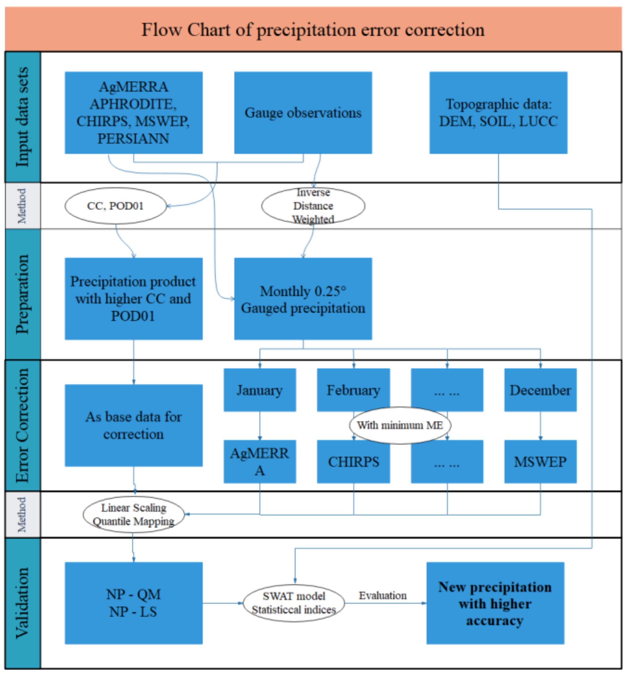
3.2. Framework of Precipitation Error Correction

In the proposed frame, the process of error correction for long-term satellite-based precipitation over poorly gauged areas can be divided into three steps, and the flow chart of this framework is shown in Figure 3. First, collect multiple sets of precipitation products with a long available period. Then, select a set of precipitation products with a high correlation coefficient and POD01 compared with gauged precipitation observation of all ground stations. The second step compares the IDW-interpolated (Inverse Distance Weighted) gauged precipitation observations with all precipitation products at each grid point, select the smallest ME product as the benchmark, and corrects the precipitation product selected the first step. The last step is to validate the corrected precipitation products using the remaining gauge observations. The detailed steps for error correction of daily precipitation are shown below:
(1)
Select multiple sets of long-term daily-scale precipitation products with high resolution.
(2)
Compare precipitation products with observed precipitation from all gauge stations, and select a set of precipitation products with a higher correlation coefficient and POD01 for correction.
(3)
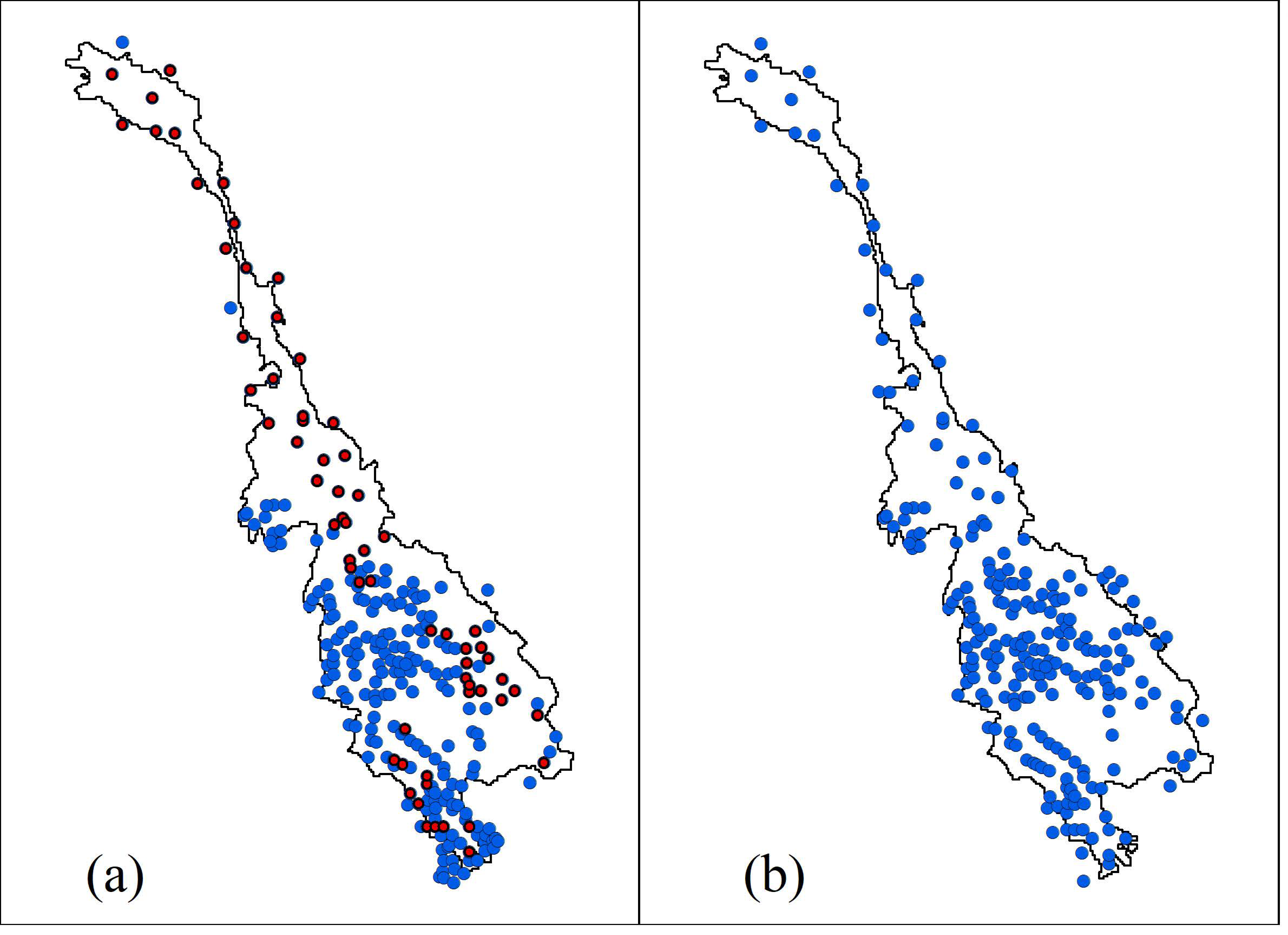
Select gauged precipitation data with a certain period (1998 to 2007 in this study) containing more stations (Figure 4), and these gauges should have better spatial representation. Then monthly grid-scale precipitation data with the same spatial resolution as the precipitation products are obtained through IDW interpolation.
(4)
Compare the IDW monthly scale precipitation data with monthly scale gauged precipitation. The precipitation product with the smallest ME at each grid point in each month is obtained as the actual rainfall value for correction.
(5)
The precipitation data obtained in the fourth step are used to correct the product selected in the second step at each grid point every month. Then the daily-scale rainfall products with higher accuracy are obtained.
(6)
Statistical indicators and hydrological simulation are used to assess the accuracy of the corrected precipitation product. In this study, the SWAT model was used for streamflow simulation.
In this study, two error correction techniques were used to remove the satellite-based precipitation product’s bias. The first technique was nonparametric empirical quantile mapping (QM) (Equation (5)) and the another was linear scaling (LS) (Equation (6)). These two techniques were used because they are easy to implement and have been proven to effectively correct daily-scale precipitation data [18,20,48]. It should be noted that the corrections in this study were performed on a monthly scale, which means that we needed to perform 12 corrections for each grid point. Following the study of Reiter et al. [49], which evaluated the rainfall corrections at multiple time scales, they found that corrections at a monthly scale were most effective in removing daily-scale precipitation bias. The calculation formulas for the two correction methods are shown below:
P r a w   =   F r a w 1   ( F c o r r ( P c o r r ) )                  
P c o r r =   P r a w   × S c a l e                     S c a l e = m e a n p e r m e a n r a w        
where P c o r r , P r a w , mean p e r and mean r a w mean precipitation of corrected, precipitation products selected in step 2, the mean value of precipitation product selected in step 4, and the mean value of precipitation product selected in step 2, respectively. F c o r r is the cumulative distribution function (CDF) of P c o r r , and F r a w 1 is the inverse CDF (or quantile function) corresponding to P r a w .

3.3. Brief Description of the SWAT Model

The SWAT is a semi-distributed hydrological model developed by the the Agricultural Research Service of the United States Department of Agriculture (USDA-ARS). It has been widely applied in various watersheds associated with climate change assessment, soil erosion, and non-point pollution [3,46,50,51]. The SWAT version 2012, coupled with the ArcGIS interface, was used in this study to evaluate the precipitation products’ performance. This model first divides the study area into several sub-basins based on the topography data sets (i.e., DEM data, mask data). Each sub-basin was discretized into multiple hydrological response units (HRUs), which are the most fundamental computational unit according to the soil type, land use data, and slope data [50,52]. The water cycle calculated by the model was simulated on each HRU. This production flow then converged to the corresponding sub-basin. Finally, the total streamflow of the study area was calculated from the output of each sub-basin. The calibration of the SWAT model was done using a separate software named SWAT-CUP (SWAT Calibration and Uncertainty Program), which can be used for calibration, validation, and uncertainty analysis of the model [52,53,54]. The SUFI-2 (Sequential Uncertainty Fitting Version 2) within the SWAT-CUP was used in this study to calibrate the model [55].
In order to evaluate the performance of the model, the Nash–Sutcliffe Efficiency coefficient (NSE) and relative bias (BIAS) (Equation (3)) were used [56]. The NSE calculation formula is shown below:
NSE   =   1     i n ( Q o i Q s i ) 2 i n ( Q o i Q ¯ o ) 2
where Q o i and Q s i represent the observed and simulated streamflow, respectively. Q ¯ o means the average of observed streamflow, and n is the total number of streamflow data.

4. Results

4.1. Evaluation of Five Precipitation Products with Gauged Observations

Spatial distributions and boxplots of the correlation coefficient for AgMERRA, APHRODITE, CHIRPS, MSWEP, and PERSIANN compared with gauged observations at a daily scale over the LMRB are shown in Figure 5. Overall, for the whole basin, APHRODITE had the best linear correlation with the gauged observations compared with the other four precipitation products (0.61 in the whole basin), followed by the MSWEP (0.49) and AgMERRA (0.39). In contrast, the CHIRPS and PERSIANN had the smallest CC (0.35). There were 204 gauges for APHRODITE with CCs more significant than 0.5, while MSWEP, AgMERRA, PERSIANN, and CHIRPS had 107, 48, 10, and 9 gauges with CC exceeding 0.5, the highest CCs for CHIRPS and PERSIANN products among all gauges were 0.54 and 0.59, respectively. In terms of the spatial distribution, gauges in China (i.e., within the Lancang River Basin) generally have higher CCs than those located in the lower LMRB. This also indicates that these five sets of precipitation products included more observation information from the gauges in the upper LRMB when they were developed.
Figure 6 shows the POD01 of five precipitation products compared with gauged observations on a daily scale. Consistent with the CC results, CHIRPS also had the smallest POD01 coefficient than the other four products. From the boxplots’ results, we can see that MSWEP was the best performing product with the highest POD01, which means that this product can most accurately predict precipitation over the LMRB. From the perspective of spatial distribution, MSWEP had the largest POD01 (higher than 0.9) in the entire LMRB, and the performance of the APHRODITE product was slightly lower than MSWEP. In contrast to the spatial performance of correlation coefficients, the POD01 of stations in the upper LMRB were lower than those in the lower LMRB, which may be affected by the complex terrain of the Qinghai–Tibet Plateau.
Figure 5 and Figure 6 show that APHRODITE and MSWEP had higher CCs and POD01 over the entire LMRB. At the same time, the prediction of precipitation occurrence was worse than MSWEP. However, considering that APHRODITE only provides daily-scale data until 2007, and Lauri et al. [28] pointed out that although APHRDOTE had a high correlation coefficient in the Mekong River Basin, there is still an underestimation of precipitation in the downstream regions. Therefore, this study chose MSWEP as the corrected precipitation product because it had a relatively high correlation coefficient compared with gauge observations and can best predict precipitation occurrence.
Figure 7 shows the spatial distribution of five precipitation products compared with IDW interpolation monthly with the smallest ME from 1998 to 2007. It can be seen from Figure 7 that no particular product can perform well in all 12 months. In general, MSWEP in the upper Qinghai–Tibet Plateau region had a better performance from January to March, May, and June. The PERSIANN performed well in April and from June to November in the middle region of the river basin. While in the downstream region, AGMERRA had a better performance from March to September. For other months and regions, no one product performed significantly better than other products. Table 3 presents the number of grids for the five precipitation products with the smallest ME over the whole basin compared with IDW-derived gauge observations at a monthly scale. We can see that from March to September, which included the rainy season of the study area, APHRODITE had the fewest grids with the smallest ME. This also means that although APHRODITE had the most massive CC compared to the other for products, its estimation of precipitation in the whole basin was not accurate. Compared with the other four products, MSWEP had the most grids with the smallest ME in February, from May to July, November, and December. In other months, AgMERRA, APHRODITE, CHIRPS, and PERSIANN performed better in September and October, January, April, and August, respectively.

4.2. Grid-Scale Evaluation of Corrected Precipitation with Gauge Observations from 1998 to 2007

Based on the results in Section 4.1 and the correction mechanism introduced in Section 3.2, we selected daily-scale MSWEP from 1979 to 2014 as the product to be corrected and used the QM and LS methods to correct the MSWEP grid by grid and month to month. The corrected precipitation is called MSWEP-QM and MSWEP-LS, respectively.
Figure 8 shows the spatial distribution of annual average precipitation derived from gauge observation, AgMERRA, APHRODITE, CHIRPS, MSWEP, PERSIANN, and two corrected products (i.e., MSWEP-QM, MSWEP-LS) from 1998 to 2007. In general, the corrected precipitation (MSWEP-QM and MSWEP-LS) can correctly represent the spatial distribution of annual-scale precipitation in the entire LMRB compared with gauge observations. The corrected products can better predict the precipitation centers of the LMRB (including the Khorat Plateau in northeastern Thailand and The Northern Highlands downstream), which is influenced by the Indian Ocean monsoon and southeast monsoon. From the spatial distribution perspective, in the upper Qinghai–Tibet Plateau, all products except PERSIANN performed well, while AgMERRA and APHRODITE underestimated annual precipitation in the middle area. In the downstream area of the LMRB, CHIRPS, MSWEP, and PERSIANN overestimated the precipitation compared to the gauge observations. For corrected precipitation, we can see that both MSWEP-QM and MSWEP-LS can better remove the precipitation error on the multi-year average scale.
Figure 9 shows the scatterplots of annual precipitation comparisons for the whole LMRB between AgMERRA, APHRODITE, CHIRPS, MSWEP, PERSIANN, MSWEP-QM, MSWEP-LS, and gauges. As shown in Figure 9, annual MSWEP-QM and MSWEP-LS agree well with gauge observations over the entire LMRB (CC = 0.97 and 0.98, respectively). Generally, for the five raw precipitation products before correction, APHRODITE underestimated the precipitation (with BIAS equals –19.01%) but had the highest CC (0.91). The CC of CHIRPS and MSWEP were also very satisfying (0.85 and 0.87, respectively) but slightly overestimated the precipitation (with BIAS equals 2.44% and 1.98%, respectively). The PERSIANN had the smallest CC, the phenomenon of overestimating the light precipitation and underestimating the heavy one existed. It should be pointed out that the original five sets of precipitation products all had a certain number of grid points that had a tendency to underestimate (overestimate) the precipitation compared with gauge observations, while the corrected precipitation products (MSWEP-QM and MSWEP-LS) effectively reduced these anomalies point (Figure 9). In conclusion, the correction mechanism proposed in this study can effectively remove the precipitation error at an annual scale, and MSWEP-QM performed slightly better than MSWEP-LS.

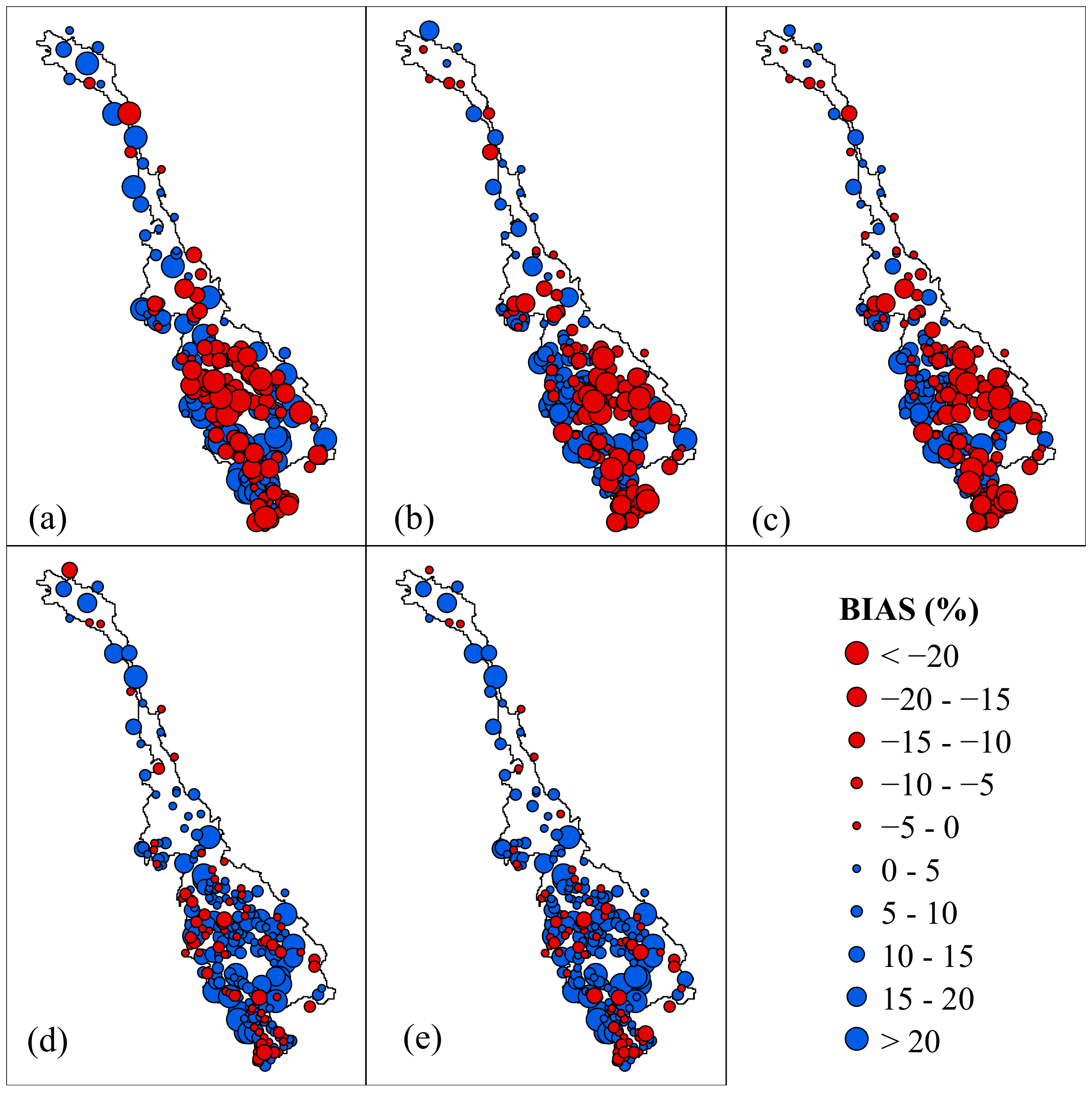
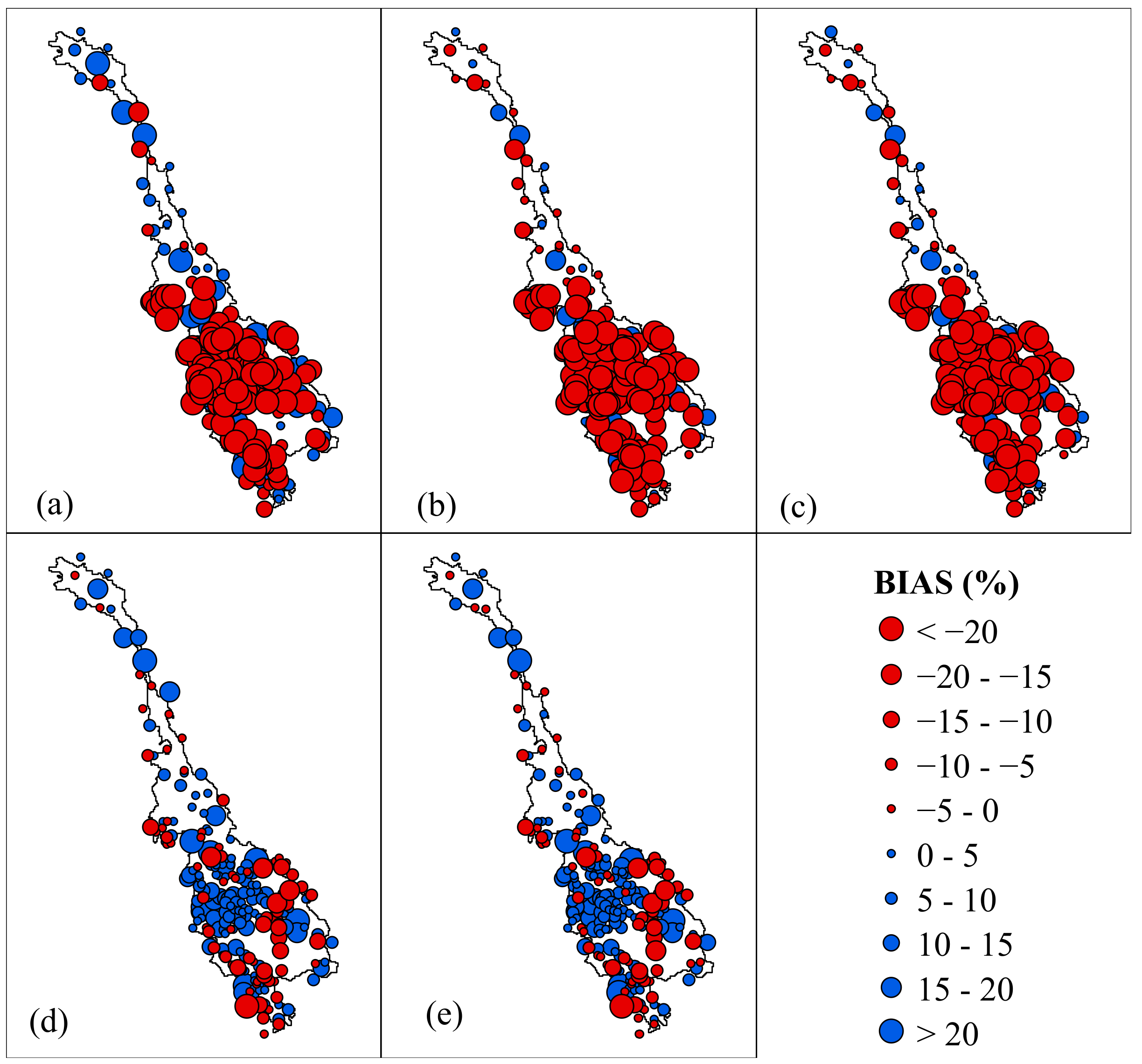
4.3. Point-Scale Evaluation of Corrected Precipitation with Gauge Observations from 1998 to 2007

In this section, we first compare the performance of two corrected precipitation products (i.e., MSWEP-QM and MSWEP-LS) with MSWEP on a daily scale from 1998 to 2007. Then the accuracy of all precipitation products with gauge observations at basin scale is conducted. Figure 10 illustrates the BIAS of (a) MSWEP, (b) MSWEP-QM, and (c) MSWEP-LS. From these three sub-figures, in general, the two corrected precipitation can effectively remove the BIAS at a daily scale in the entire LMRB. However, there is still relatively large BIAS in high-altitude areas in the southeast of the basin and the Mekong Delta region; this may be due to the short data sequence of the gauges in these two regions to some errors in the IDW interpolation precipitation. By comparing the two corrected rainfall products, we can see that MSWEP-LS performed slightly better than MSWEP-QM in the upper Qinghai–Tibet Plateau and performed exceptionally well in other parts the river basin. Among 246 evaluated gauges, MSWEP-LS and MSWEP-QM had 214 and 211 gauges with BIAS between –20% and 20%, while MSWEP had 183 gauges. Figure 10d,e show the changes in the BIAS of MSWEP-QM and MSWEP-LS compared to MSWEP products. The MSWEP-QM and MSWEP-LS products had 165 and 171 gauges of BIAS, showing a decreasing trend, respectively. For the remaining stations, the amount of BIAS change was also less than 10%. From the average BIAS of all gauges, the average BIAS of MSWEP-QM and MSWEP-LS reached 0.17% and –0.5%, respectively, which significantly reduced the average BIAS of MSWEP (2.48%). The average absolute BIAS of all gauges of MSWEP-QM and MSWEP-LS also decreased from 16.57% to 11.21% and 10.69%. Generally, the corrected precipitation products can perform better than MSWEP at most stations, and MSWEP-LS performs slightly better than MSWEP-QM.
Figure 11 shows scatterplots of precipitation estimate comparisons for the entire LMRB at a daily scale between AgMERRA, APHRODITE, CHIRPS, MSWEP, PERSIANN, MSWEP-QM, MSWEP-LS, and gauge observations from 1998 to 2007. Precipitation values were calculated from the arithmetic mean of the precipitation at the grid points that contain those stations, and gauge observations over the LMRB at a daily scale, respectively. As shown in Figure 11, APHRODITE has the largest correlation coefficient than gauge observations. However, it also has the most extensive BIAS (–15.5%), consistent with the results shown in Figure 8 and Figure 9. The PERSIANN had the smallest CC (0.79) and R-Square (0.62), and relatively large BIAS (10.44%), which is also consistent with the results in Figure 5 and Table 3, which means that there are a relatively large number of grids points for accurate precipitation estimation. For corrected precipitation products, MSWEP-QM had a smaller BIAS and almost equal CC and R-Square than MSWEP, and MSWEP-LS had slightly larger CC and R-Square than MSWEP. However, the absolute value of its BIAS increased slightly. The higher BIAS was probably caused by the cancelation of positive and negative values. Overall, the corrected precipitation products can slightly increase the CC and reduce the BIAS at the whole river basin scale.

4.4. Hydrological and Regional Evaluation of Corrected Precipitation from 1998 to 2007

Hydrological and regional evaluations are conducted in this section to evaluate the performance of corrected precipitation products. We first used the gauge observations from 1998 to 2007 to calibrate the SWAT model, and then the calibrated model was used to assess the accuracy of all precipitation products. The regional evaluation was conducted in seven zones which were divided into six hydrological stations (Figure 1), namely, Y (above Yunjinghong station), YC (from Yunjinghong to Chiang Saen), CL (from Chiang Saen to Luang Prabang), LM (from Luang Prabang to Mukdahan), MP (from Mukdahan to Pakse), PS (from Pakse to Stung Treng). and SD (from Stung Treng to Mekong Delta).
Table 4 shows the SWAT model’s simulation results at six selected hydrological stations with all eight precipitation inputs (including gauge observations). The results indicate that this model has good adaptability in the entire LMRB. For the five precipitation products, in general, the simulation results at the Yunjinghong station were the worst compared to other stations. Even though the NSE coefficient of MSWEP product reached 0.8, it had a relatively large BIAS (15.07%). For the other five stations, APHRODITE mostly underestimated the streamflow (except the Luang Prabang station), which was also consistent with the results presented in Figure 8 and Figure 11. The AgMERRA, CHIRPS, MSWEP, and PERSIANN all had large negative BIAS at the Mukdahan station. Through Figure 8, we can see that these four products all underestimated the precipitation. As for the corrected precipitation products, we can see that the MSWEP-LS showed better performance than the MSWEP product in five of the six stations, while MSWEP-QM had better simulation results than MSWEP in just two stations. In summary, the corrected MSWEP-LS product can better simulate the daily streamflow processes in the entire LMRB (with all NSE greater than 0.8 and all BIAS lower than 11.4). To further explain the simulation results presented in Table 4 and evaluate the corrected rainfall product’s accuracy, the regional evaluation was conducted next.
Table 5 shows the BIAS of five precipitation products (i.e., AgMERRA, APHRODITE, CHIRPS, MSWEP, and PERSIANN) and two corrected precipitation products (MSWEP-QM and MSWEP-LS) against gauge observations over seven sub-regions at a daily scale from 1998 to 2007. Overall, the BIAS of the two corrected precipitation products is within ±9%, which means that the framework proposed in this study can effectively remove the precipitation errors on a sub-regional scale. From a spatial perspective, the two corrected products all have smaller BIAS in Y, YC, PS, and SD regions than the original five precipitation products. In contrast, in the other two regions, the BIAS was slightly larger than the MSWEP product. From the performance of different rainfall products and their impact on hydrological simulation results, we can see that APHRODITE underestimates the precipitation in all seven sub-regions. The underestimation of precipitation led to the underestimated flow process of this product’s hydrological simulation results (Table 4). The PERSAINN had a 20.99% precipitation error in the Y region, resulting in a larger BIAS (49.51%) for its streamflow simulation. In general, the two corrected products showed a smaller BIAS in the four sub-regions (Y, YC, PS, and SD) than the original five rainfall products, while the BIAS in the other three sub-regions shows a small increase. This may be related to the offset of the positive and negative BIAS values at different gauges. The results in Figure 10 indicate that the corrected precipitation data decreased BIAS at most gauges.

4.5. Validation of Corrected Precipitation with Gauge Observations from 1979 to 1997 and 2008 to 2014

In the previous sections, we evaluated the corrected precipitation products at the point scale and grid-scale from 1998 to 2007. This section evaluates the corrected precipitation products on the remaining observations (i.e., from 1979 to 1997 and 2008 to 2014) to assess the performance of the bias correction framework proposed in this study.
Figure 12a–c show the BIAS of MSWEP, MSWEP-QM, and MSWEP-LS compared with gauge observation on a daily scale from 1979 to 1997 and 2008 to 2014. From these three subfigures, we can see that the two sets of corrected precipitation products have smaller BIAS compared to MSWEP in the upper Mekong River Basin. However, most stations downstream still showed a tendency to underestimate precipitation. The cause of this phenomenon may be that these sets of precipitation products only contained information on the limited ground observation gauges in the downstream area during the generation process. We further compared the BIAS changes at a daily scale between the MSWEP-QM (d), MSWEP-LS (e), and MSWEP. The results showed that the corrected precipitation products can effectively reduce BIAS at most stations, especially in the upstream and middle reaches. However, BIAS in some high-altitude areas in the southeast of the basin and some Mekong Delta stations showed a larger trend. The average absolute BIAS of MSWEP was 21.4%, and the corrected MSWEP-QM and MSWEP-LS were 17.98% and 17.87%, which were reduced by 3.4% and 3.51%, respectively.

5. Discussion

5.1. Performance of Different Precipitation Products

In this study, before error correction of the precipitation products, we first evaluated five precipitation products (i.e., AgMERRA, APHRODITE, CHIRPS, MSWEP, and PERSIANN). Then, we compared them with gauge observations in the Lancang-Mekong River Basin mainly from three aspects (correlation coefficient, probability of detection, and mean error of each month). We found that APHRODITE had the largest correlation coefficient among the five products (followed by MSWEP, AgMERRA, PERSIANN, and CHIRPS) in the LMRB (Figure 5), and this conclusion is consistent with the previous research results of the LMRB [28,33]. However, at the same time, we also found that APHRODITE had severely underestimated precipitation (Figure 8 and Figure 11), especially in the lower LMRB. The underestimated precipitation also led to underestimating the hydrological simulation of the runoff processes (Table 5), and this conclusion was rarely mentioned in published studies. Although the development of the APHRODITE precipitation product included 5000–12,000 verification stations in Asia, the monthly precipitation data in this study area only included ground gauges in Thailand and the Lancang River area in China [44]. This may be one of the reasons for its poor performance in the downstream area of LMRB. On the other hand, Figure 6 in the original article published on the development of the APHRODITE [44] compared the annual average precipitation of APHRODITE and Global Precipitation Climatology Centre (GPCC) from 1961 to 2004, and the result also indicates that the precipitation in the lower LMRB was underestimated. However, due to the fact tjat surface observation data in the LMRB are scarce and difficult to collect, the APHRODITE has always been selected as the actual precipitation values in many published studies without considering its errors [28,31]. As these References [46,57] have shown, any small precipitation error may be amplified by hydrological simulations and affect the entire water resource allocation, sustainable development strategy formulation, etc. For the accuracy of precipitation event detection (including precipitation equal to 0), we can see that MSWEP had the best performance over the other four products, followed by APHRODITE. This is because the MSWEP product uses a weighted average of seven rainfall products (i.e., CPC Unified, GPCC, CMORPH, GSMaP-MVK, TMPA 3B42V7, ERA-Interim, and JRA-55) during the development process [10]. It also uses the average precipitation and streamflow of 13,762 watersheds worldwide to remove the impact of terrain on precipitation. The AgMERRA mainly uses data sets of MERRA-Land and wet days of CRU to correct the precipitation days [42,58]. Whereas CHIRPS uses the CHPclim model to integrate the FAO and Global Historical Climate Network (GHCN) stations, remote sensing data TMPA and CMORPH [59]. The PERSIANN mainly uses GPCP monthly average precipitation to correct its product [40]. That means that the MSWEP incorporates more information about precipitation products and ground stations, which may be an important reason for its more accurate detection of rainfall events. We understand why MSWEP has the most grids in more months (February, May, June, July, November, and December) to estimate precipitation more accurately than the other four products (Table 3). However, as shown in Figure 7 and Figure 8, MSWEP still has large errors in some areas of the LMRB. Therefore, in this study, we propose a bias correction mechanism based on various remote sensing and reanalysis precipitation products, hoping to provide a set of long-range precipitation products with high accuracy for the LMRB.

5.2. Applicability of the Error Correction Framework

The error correction framework proposed in this study using Quantile Mapping (QM) and Linear Scaling (LS) both fit quite well with smaller ME and BIAS in most stations, and it can also better spatially predict the precipitation in the entire LMRB (Figure 6 and Figure 7). Because we first select the precipitation product based on the CC and rainfall events estimates (POD01), and then further corrects the precipitation errors. Therefore, after correction, we use BIAS, which focuses on its estimation of quantity for the precipitation assessment. From the corrected rainfall products’ evaluation results, MSWEP-LS is slightly better than MSWEP-QM, mainly due to the two correction methods’ different internal mechanisms. Because the QM method uses the cumulative precipitation distribution function (CDF) to correct the selected product (MSWEP in this study) by one percentile. However, in this study, we selected the precipitation product with the smallest ME at each grid point in each month as the benchmark. There may be errors between the cumulative distribution curve and those of station observations. The LS method only uses a scaling factor to correct the precipitation. MSWEP has a higher correlation coefficient than the site-observed precipitation in the LMRB, which may be one reason why the MSWEP-LS method performs slightly better than MSWEP-QM. Ghimire et al. [18] compared and analyzed the effects of LS and QM methods on streamflow simulation after global climate models (GCMs) precipitation product bias correction, and they found that the LS method showed better performance than QM. As shown in Figure 9, the BIAS of MSWEP-QM was slightly smaller than that of MSWEP-LS. However, the results shown in Figure 8 indicate that the BIAS of MSWEP-LS had more stations showing a decreasing trend, which is probably caused by the cancelation of positive and negative values [60]. We have not achieved perfect results in LM (from Luang Prabang to Mukdahan) and MP (from Mukdahan to Pakse) regions from the regional evaluation results. This setback is partly due to the shorter available data length of the stations we collected in these two regions, which led to our IDW interpolation results in these areas may be insufficient. In general, although this study was conducted in the Lancang-Mekong River Basin, the proposed framework could also be applicable in other areas, especially for those with limited gauge observations.

5.3. Limitations and Future Directions of This Study

Although the framework proposed in this study can effectively remove the BIAS of precipitation on a daily scale over the entire LMRB (Figure 8, Figure 10 and Figure 12), there are also limitations. In this study, the IDW interpolation method was used to obtain the grid-scale (0.25°) monthly precipitation with observed precipitation from 1998 to 2007. However, there is no doubt that interpolation will bring some errors [33], especially in the lower LMRB where the gauges have shorter data sequences available. In future research, we should collect more ground radar and gauge observation data to reduce further the errors caused by interpolation. Second, due to the difficulty of collecting the observation data of LMRB and the available data series are always short, in this study, the product with the smallest mean error was selected as the actual value at each grid point each month, in other words, the accuracy of the remote sensed or reanalysis precipitation product at a specific grid point has a greater contribution to the accuracy of the corrected precipitation than the gauge observations. However, it is clear that each product inevitably has specific errors compared to gauge observations [8,61], making it impossible for us to remove the precipitation error using the available data we collected. Third, the correction result is also related to the spatial distribution of the collected rainfall stations. From the Figure 8, we can see that in the eastern mountainous area of the lower reaches of the LMRB, the corrected precipitation products can better present the annual rainfall distribution of the basin compared with the gauge observations, but in the lower reaches of Cambodia, the observation data we collected by the ground rainfall stations in this area is very limited, therefore, there may still be some uncertainty in the corrected precipitation in this area (Figure 8). In the last aspect, our study used mean error as the unique indicator to select the precipitation products as the actual value; as concluded by Wang et al. [62], extreme precipitation is more meaningful for the prediction of water-related disasters and the sustainable use of water resources in the watershed. Therefore, in the next research, we should consider extreme precipitation indicators when selecting precipitation products. However, as we have shown in our introduction and results, our proposed framework can reduce the BIAS of MSWEP at most gauges. According to Figure 10, Figure 11 and Figure 12, both the MSWEP-QM and MSWEP-LS performed better than the raw precipitation products (i.e., AgMERRA, APHRODITE, CHIRPS, MSWEP, and PERSIANN), of which MSWEP-LS performs better. Therefore, we recommend that MSWEP-LS be used for related studies such as hydrological simulation in the Lancang-Mekong River Basin.

6. Conclusions

In this study, we proposed and implemented a novel daily-scale precipitation bias correction framework based on multiple long-term remote sensing and reanalysis precipitation products in Lancang-Mekong River Basin, which also can be used in other poorly gauged areas. We first compared the five rainfall products (i.e., AgMERRA, APHRODITE, CHIRPS, MSWEP, and PERSIANN) with the observed precipitation. The resulting precipitation products MSWEP-QM derived from quantile mapping and MSWEP-LS derived from linear scaling were evaluated in calibration (from 1998 to 2007) and validation (1979 to 1997 and 2008 to 2014) periods. The main conclusions are summarized in the following points:
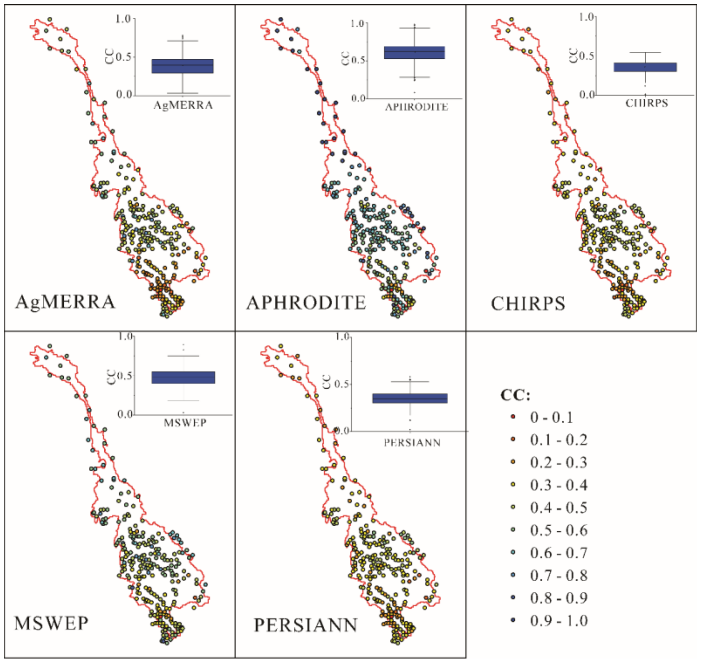
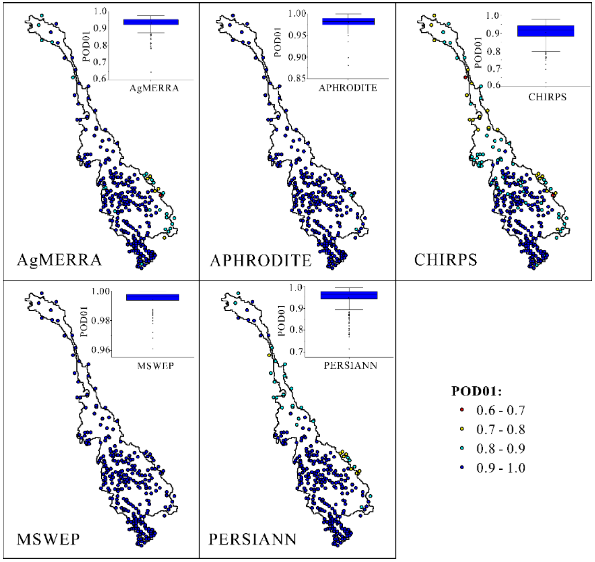
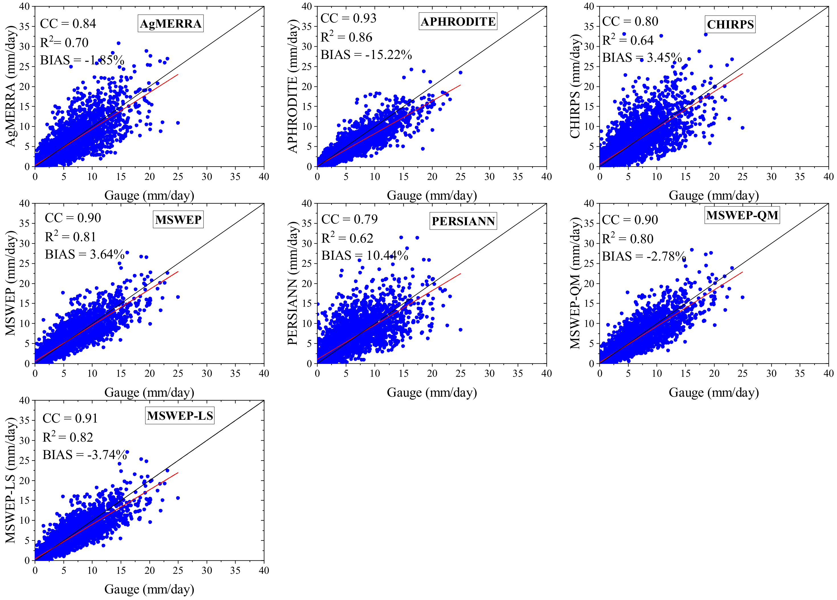
  • The APHRODITE showed the highest CC (0.61) with gauge observations at a daily scale but greatly underestimated the precipitation (with BIAS equals –15.5%), especially in the downstream areas. This means that we should carefully choose APHRODITE as the actual value of the LMRB for related research. The average probability of precipitation detection (POD01) estimated by MSWEP was 0.99, which was the highest among the five raw precipitation products.
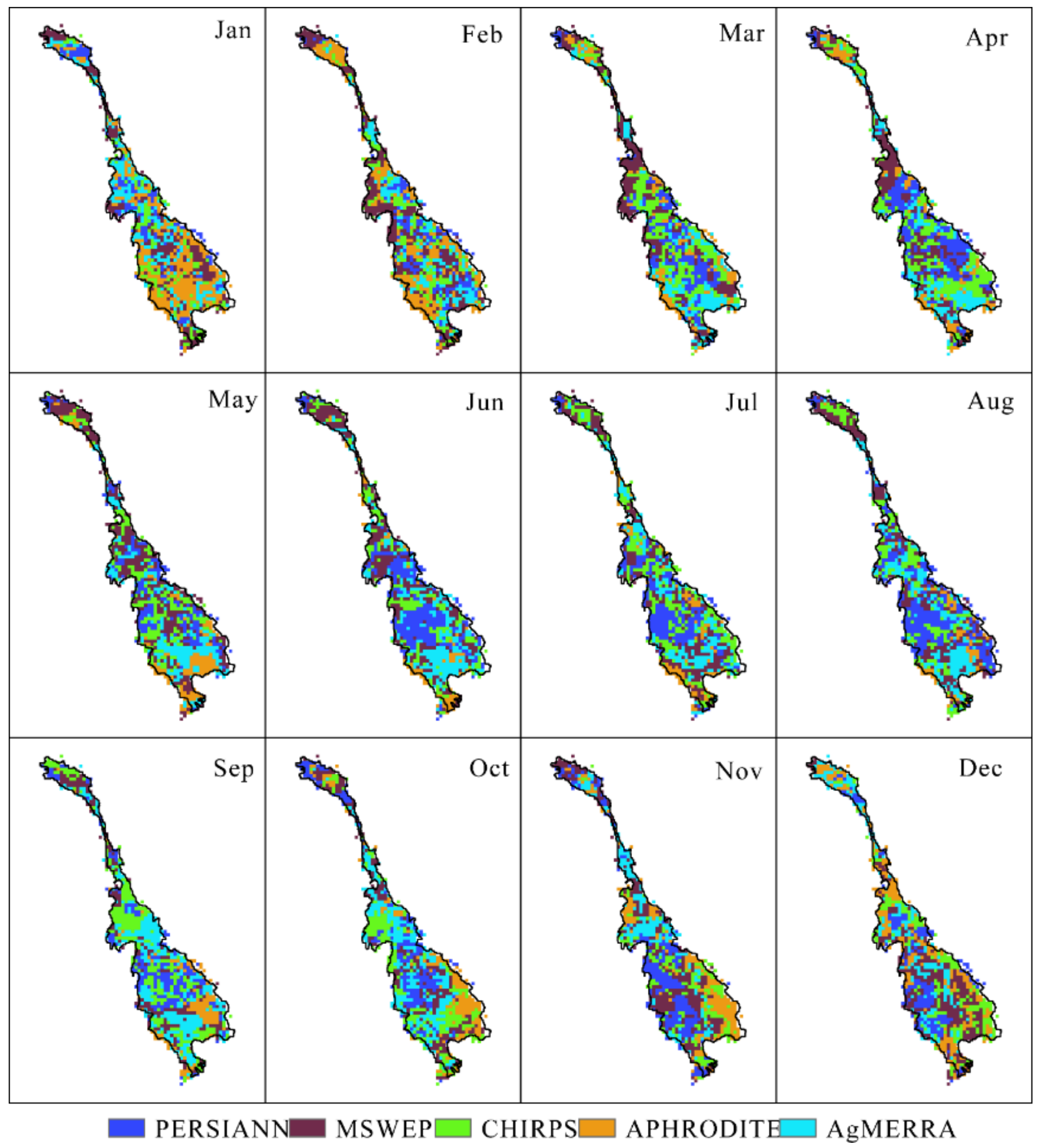
  • The monthly grid-scale evaluation results showed that most grids of MSWEP had the smallest ME in February, from May to July, November, and December. The AgMERRA, APHRODITE, CHIRPS, and PERSIANN had the most grids with the smallest ME in September and October, January, April, and August, respectively. The variation of five precipitation products’ performance over the entire LMRB was associated with the data sources included in their respective development processes and the different algorithms they adopt.
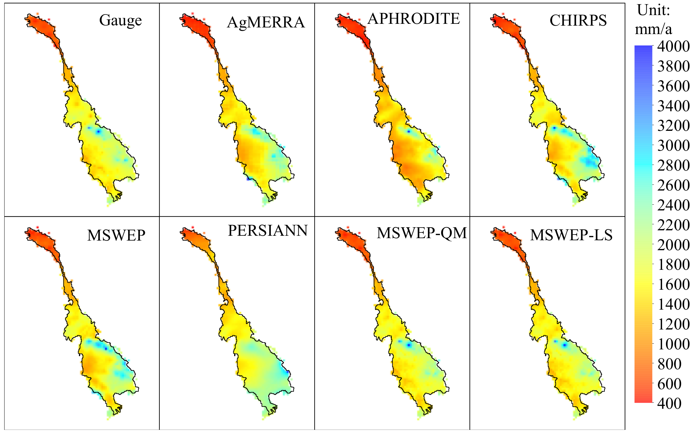
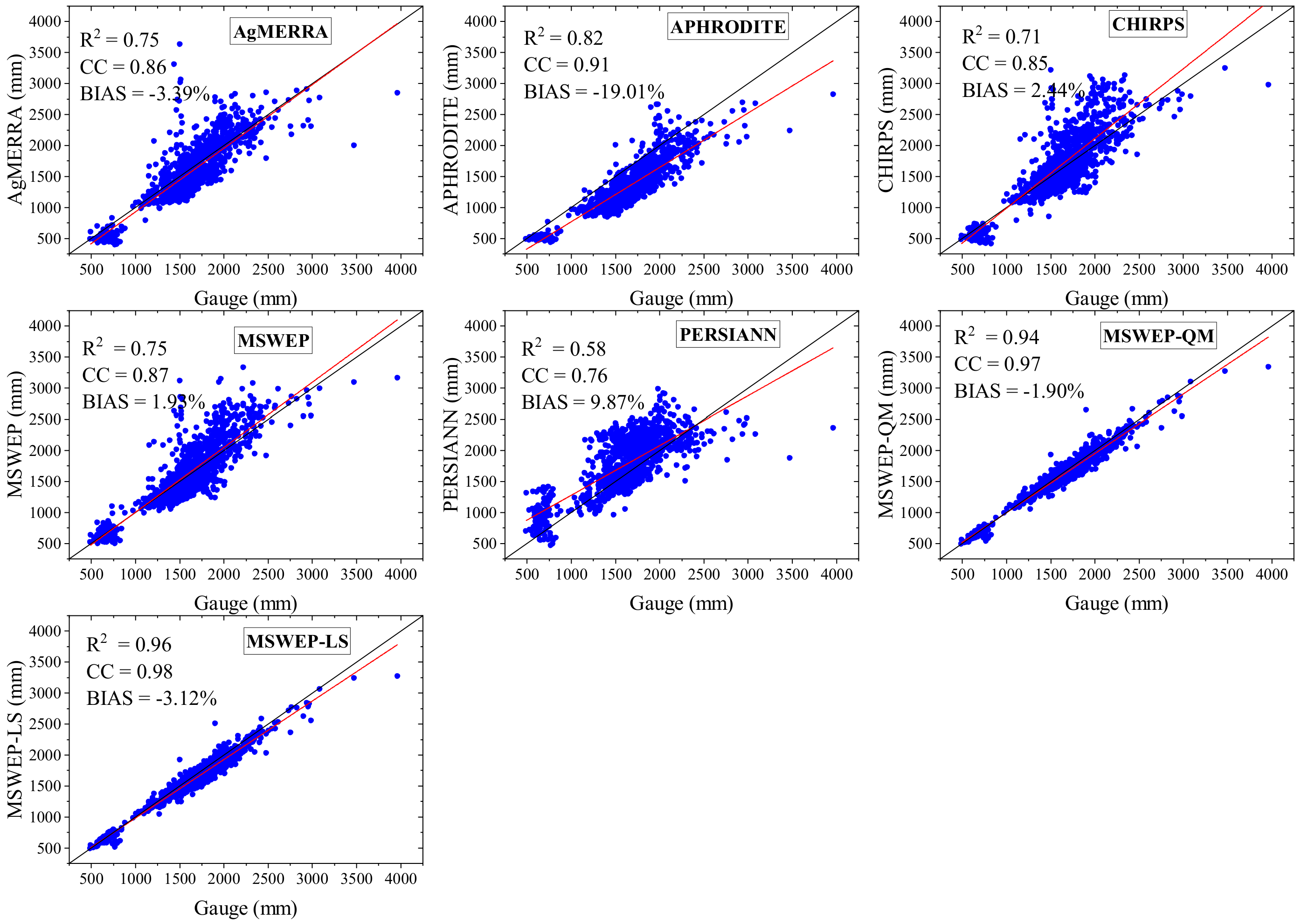
  • Grid-scale evaluation shows that two resulting precipitation products both can capture the spatial variability of multi-year average precipitation across the entire LMRB in the calibration period. The MSWEP-QM (0.97) and MSWEP-LS (0.98) have higher CC than AgMRRA (0.86), APHRODITE (0.91), CHIRPS (0.86), MSWEP (0.87), PERSIANN (0.76). The point-scale evaluation results indicate that the BIAS of MSWEP-QM (165 in 246), and MSWEP-LS (171 in 246) have more gauges showing a downward trend.
  • Hydrological and regional revaluation shows that MSWEP-LS and MSWEP-QM achieved better simulation results in five regions (i.e., Y, YC, CL, LM, and MP regions) compared to the two regions derived from MSWEP (LM and MP). The BIAS of MSWEP-QM and MSWEP-LS in seven sub-regions all reach within ±9% on a daily scale. They also had smaller BIAS in Y, YC, PS, and SA regions than the five raw precipitation products.
  • Validation results indicated that the average absolute BIAS of MSWEP-QM and MSWEP-LS reduced by 3.4% and 3.51%, respectively, compared to MSWEP. The BIAS of MSWEP-QM and MSWEP-LS had 141 and 142 gauges showing a decreasing trend than MSWEP.
In general, the novel precipitation bias-correction framework proposed in this study is considered to provide a viable study for blending five selected precipitation products in regions with limited gauge observations. We also recommend that the MSWEP-LS can be used for further water-related research in LMRB.

Author Contributions

Conceptualization, X.T. and G.W.; methodology, X.T.; writing—original draft preparation, X.T.; writing—review and editing, G.B.R., J.Z., Z.B., Y.L., C.L., and J.J. All authors have read and agreed to the published version of the manuscript.

Funding

This study was funded by the National Key Research and Development Plan of China (grant number: 2016YFA0601501), the National Natural Science Foundation of China (grant number: 41830863) and the National Key Research and Development Plan of China (grant number: 2017YFC0405604).

Institutional Review Board Statement

Not applicable.

Informed Consent Statement

Not applicable.

Data Availability Statement

The data presented in this study are available on request from the corresponding author.

Acknowledgments

The authors are very grateful to all anonymous reviewers, chief editors and associate editors for their valuable comments and suggestions, which not only greatly improved the quality of this paper but also have immense value for our future research.

Conflicts of Interest

The authors declare no competing interests.

References

  1. Duan, Z.; Bastiaanssen, W. First results from Version 7 TRMM 3B43 precipitation product in combination with a new downscaling-calibration procedure. Remote Sens. Environ. 2013, 131, 1–13. [Google Scholar] [CrossRef]
  2. Gao, C.; Booij, M.J.; Xu, Y.P. Impacts of climate change on characteristics of daily-scale rainfall events based on nine selected GCMs under four CMIP5 RCP scenarios in Qu River basin, east China. Int. J. Climatol. 2020, 40, 887–907. [Google Scholar] [CrossRef]
  3. Zhu, Q.; Hsu, K.l.; Xu, Y.P.; Yang, T. Evaluation of a new satellite-based precipitation data set for climate studies in the Xiang River basin, southern China. Int. J. Climatol. 2017, 37, 4561–4575. [Google Scholar] [CrossRef]
  4. Tang, G.; Long, D.; Hong, Y.; Gao, J.; Wan, W. Documentation of multifactorial relationships between precipitation and topography of the Tibetan Plateau using spaceborne precipitation radars. Remote Sens. Environ. 2018, 208, 82–96. [Google Scholar] [CrossRef]
  5. Tang, X.; Zhang, J.; Gao, C.; Ruben, G.B.; Wang, G. Assessing the Uncertainties of Four Precipitation Products for Swat Modeling in Mekong River Basin. Remote Sens. 2019, 11, 304. [Google Scholar] [CrossRef] [Green Version]
  6. Luo, X.; Wu, W.; He, D.; Li, Y.; Ji, X. Hydrological Simulation Using TRMM and CHIRPS Precipitation Estimates in the Lower Lancang-Mekong River Basin. Chin. Geogr. Sci. 2019, 29, 13–25. [Google Scholar] [CrossRef] [Green Version]
  7. Wang, W.; Lu, H.; Yang, D.; Khem, S.; Yang, J.; Gao, B.; Peng, X.; Pang, Z. Modelling Hydrologic Processes in the Mekong River Basin Using a Distributed Model Driven by Satellite Precipitation and Rain Gauge Observations. PLoS ONE 2016, 11, e0152229. [Google Scholar] [CrossRef] [Green Version]
  8. Yong, B.; Chen, B.; Gourley, J.J.; Ren, L.; Hong, Y.; Chen, X.; Wang, W.; Chen, S.; Gong, L. Intercomparison of the Version-6 and Version-7 TMPA precipitation products over high and low latitudes basins with independent gauge networks: Is the newer version better in both real-time and post-real-time analysis for water resources and hydrologic extremes? J. Hydrol. 2014, 508, 77–87. [Google Scholar] [CrossRef]
  9. Huffman, G.J.; Bolvin, D.T.; Nelkin, E.J.; Wolff, D.B.; Adler, R.F.; Gu, G.; Hong, Y.; Bowman, K.P.; Stocker, E.F. The TRMM multisatellite precipitation analysis (TMPA): Quasi-global, multiyear, combined-sensor precipitation estimates at fine scales. J. Hydrometeorol. 2007, 8, 38–55. [Google Scholar] [CrossRef]
  10. Beck, H.E.; Van Dijk, A.I.J.M.; Levizzani, V.; Schellekens, J.; Miralles, D.G.; Martens, B.; De Roo, A. MSWEP: 3-hourly 0.25° global gridded precipitation (1979–2015) by merging gauge, satellite, and reanalysis data. Hydrol. Earth Syst. Sci. 2016, 21, 1–38. [Google Scholar] [CrossRef] [Green Version]
  11. Mazzoleni, M.; Brandimarte, L.; Amaranto, A. Evaluating precipitation datasets for large-scale distributed hydrological modelling. J. Hydrol. 2019, 578, 124076. [Google Scholar] [CrossRef] [Green Version]
  12. Yatagai, A.; Kamiguchi, K.; Arakawa, O.; Hamada, A.; Yasutomi, N.; Kitoh, A. APHRODITE: Constructing a Long-Term Daily Gridded Precipitation Dataset for Asia Based on a Dense Network of Rain Gauges. Bull. Am. Meteorol. Soc. 2012, 93, 1401–1415. [Google Scholar] [CrossRef]
  13. Tang, X.; Zhang, J.; Wang, G.; Yang, Q.; Yang, Y.; Guan, T.; Liu, C.; Jin, J.; Liu, Y.; Bao, Z. Evaluating Suitability of Multiple Precipitation Products for the Lancang River Basin. Chin. Geogr. Sci. 2019, 29, 37–57. [Google Scholar] [CrossRef] [Green Version]
  14. Ma, Y.; Hong, Y.; Chen, Y.; Yang, Y.; Tang, G.; Yao, Y.; Long, D.; Li, C.; Han, Z.; Liu, R. Performance of optimally merged multisatellite precipitation products using the dynamic Bayesian model averaging scheme over the Tibetan Plateau. J. Geophys. Res. Atmos. 2018, 123, 814–834. [Google Scholar] [CrossRef]
  15. Worqlul, A.W.; Ayana, E.K.; Maathuis, B.H.P.; Macalister, C.; Philpot, W.D.; Leyton, J.M.O.; Steenhuis, T.S. Performance of bias corrected MPEG rainfall estimate for rainfall-runoff simulation in the upper Blue Nile Basin, Ethiopia. J. Hydrol. 2017, 556, S0022169417300689. [Google Scholar] [CrossRef]
  16. Gutjahr, O.; Heinemann, G. Comparing precipitation bias correction methods for high-resolution regional climate simulations using COSMO-CLM. Theor. Appl. Clim. 2013, 114, 511–529. [Google Scholar] [CrossRef]
  17. Gudmundsson, L.; Bremnes, J.; Haugen, J.; Engen-Skaugen, T. Downscaling RCM precipitation to the station scale using statistical transformations—A comparison of methods. Hydrol. Earth Syst. Sci. 2012, 16, 3383–3390. [Google Scholar] [CrossRef] [Green Version]
  18. Ghimire, U.; Srinivasan, G.; Agarwal, A. Assessment of rainfall bias correction techniques for improved hydrological simulation. Int. J. Climatol. 2019, 39, 2386–2399. [Google Scholar] [CrossRef]
  19. Habib, E.; Haile, A.; Sazib, N.; Zhang, Y.; Rientjes, T. Effect of Bias Correction of Satellite-Rainfall Estimates on Runoff Simulations at the Source of the Upper Blue Nile. Remote Sens. 2014, 6, 6688–6708. [Google Scholar] [CrossRef] [Green Version]
  20. Gumindoga, W.; Rientjes, T.H.; Haile, A.T.; Makurira, H.; Reggiani, P. Performance of bias-correction schemes for CMORPH rainfall estimates in the Zambezi River basin. Hydrol. Earth Syst. Sci. 2019, 23, 2915–2938. [Google Scholar] [CrossRef] [Green Version]
  21. Boushaki, F.I.; Hsu, K.-L.; Sorooshian, S.; Park, G.-H.; Mahani, S.; Shi, W. Bias adjustment of satellite precipitation estimation using ground-based measurement: A case study evaluation over the southwestern United States. J. Hydrometeorol. 2009, 10, 1231–1242. [Google Scholar] [CrossRef]
  22. Xie, P.; Xiong, A.Y. A conceptual model for constructing high-resolution gauge-satellite merged precipitation analyses. J. Geophys. Res. Atmos. 2011, 116. [Google Scholar] [CrossRef]
  23. Li, Y.; Zhang, Y.; He, D.; Luo, X.; Ji, X. Spatial downscaling of the tropical rainfall measuring mission precipitation using geographically weighted regression Kriging over the Lancang River Basin, China. Chin. Geogr. Sci. 2019, 29, 446–462. [Google Scholar] [CrossRef] [Green Version]
  24. Mahmood, R.; Jia, S.; Tripathi, N.K.; Shrestha, S. Precipitation extended linear scaling method for correcting GCM precipitation and its evaluation and implication in the transboundary Jhelum River basin. Atmosphere 2018, 9, 160. [Google Scholar] [CrossRef] [Green Version]
  25. Maraun, D. Bias correction, quantile mapping, and downscaling: Revisiting the inflation issue. J. Clim. 2013, 26, 2137–2143. [Google Scholar] [CrossRef] [Green Version]
  26. Liu, S.; Yan, D.; Qin, T.; Weng, B.; Li, M. Correction of TRMM 3B42V7 based on linear regression models over China. Adv. Meteorol. 2016, 2016. [Google Scholar] [CrossRef]
  27. Hecht, J.S.; Lacombe, G.; Arias, M.E.; Dang, T.D.; Piman, T. Hydropower dams of the Mekong River basin: A review of their hydrological impacts. J. Hydrol. 2018, 568, 285–300. [Google Scholar] [CrossRef]
  28. Lauri, H.; Räsänen, T.A.; Kummu, M. Using Reanalysis and Remotely Sensed Temperature and Precipitation Data for Hydrological Modeling in Monsoon Climate: Mekong River Case Study. J. Hydrometeorol. 2014, 15, 1532–1545. [Google Scholar] [CrossRef]
  29. Winemiller, K.O.; Mcintyre, P.B.; Castello, L.; Fluetchouinard, E.; Giarrizzo, T.; Nam, S.; Baird, I.G.; Darwall, W.; Lujan, N.K.; Harrison, I. Development and environment. Balancing hydropower and biodiversity in the Amazon, Congo, and Mekong. Science 2016, 351, 128. [Google Scholar] [CrossRef] [Green Version]
  30. Ohara, N.; Chen, Z.; Kavvas, M.; Fukami, K.; Inomata, H. Reconstruction of historical atmospheric data by a hydroclimate model for the Mekong River basin. J. Hydrol. Eng. 2010, 16, 1030–1039. [Google Scholar] [CrossRef]
  31. Chen, A.; Chen, D.; Azorin-Molina, C. Assessing reliability of precipitation data over the Mekong River Basin: A comparison of ground-based, satellite, and reanalysis datasets. Int. J. Climatol. 2018, 38, 4314–4334. [Google Scholar] [CrossRef]
  32. Chen, C.; Jayasekera, D.; Senarath, S. Assessing Uncertainty in Precipitation and Hydrological Modeling in the Mekong. In Proceedings of the World Environmental and Water Resources Congress, Austin, TX, USA, 17–21 May 2015; pp. 2510–2519. [Google Scholar]
  33. Chen, C.J.; Senarath, S.U.S.; Dima-West, I.M.; Marcella, M.P. Evaluation and restructuring of gridded precipitation data over the Greater Mekong Subregion. Int. J. Climatol. 2016, 37, 180–196. [Google Scholar] [CrossRef]
  34. Zhang, J.; Fan, H.; He, D.; Chen, J. Integrating precipitation zoning with random forest regression for the spatial downscaling of satellite-based precipitation: A case study of the Lancang-Mekong River basin. Int. J. Climatol. 2019, 39, 3947–3961. [Google Scholar] [CrossRef]
  35. Jacobs, J.W. The Mekong River Commission: Transboundary Water Resources Planning and Regional Security. Geogr. J. 2002, 168, 354–364. [Google Scholar] [CrossRef] [PubMed]
  36. Han, Z.; Long, D.; Fang, Y.; Hou, A.; Hong, Y. Impacts of climate change and human activities on the flow regime of the dammed Lancang River in Southwest China. J. Hydrol. 2019, 570, 96–105. [Google Scholar] [CrossRef]
  37. Li, D.; Long, D.; Zhao, J.; Lu, H.; Hong, Y. Observed changes in flow regimes in the Mekong River basin. J. Hydrol. 2017, 551, 217–232. [Google Scholar] [CrossRef]
  38. Ruane, A.C.; Goldberg, R.; Chryssanthacopoulos, J. Climate forcing datasets for agricultural modeling: Merged products for gap-filling and historical climate series estimation. Agric. For. Meteorol. 2015, 200, 233–248. [Google Scholar] [CrossRef] [Green Version]
  39. Retalis, A.; Tymvios, F.; Katsanos, D.; Michaelides, S. Downscaling CHIRPS precipitation data: An artificial neural network modelling approach. Int. J. Remote Sens. 2017, 38, 3943–3959. [Google Scholar] [CrossRef]
  40. Faridzad, M.; Yang, T.; Hsu, K.; Sorooshian, S.; Xiao, C. Rainfall Frequency Analysis for Ungauged Regions using Remotely Sensed Precipitation Information. J. Hydrol. 2018, 563, 123–142. [Google Scholar] [CrossRef] [Green Version]
  41. Reichle, R.H.; Koster, R.D.; De Lannoy, G.J.M.; Forman, B.A.; Liu, Q.; Mahanama, S.P.P.; Touré, A. Assessment and Enhancement of MERRA Land Surface Hydrology Estimates. J. Clim. 2011, 24, 6322–6338. [Google Scholar] [CrossRef] [Green Version]
  42. Rienecker, M.M.; Suarez, M.J.; Gelaro, R.; Todling, R.; Bacmeister, J.; Liu, E.; Bosilovich, M.G.; Schubert, S.D.; Takacs, L.; Kim, G.K. MERRA: NASA’s Modern-Era Retrospective Analysis for Research and Applications. J. Clim. 2011, 24, 3624–3648. [Google Scholar] [CrossRef]
  43. Rienecker, M.M.; Suarez, M.J.; Todling, R.; Bacmeister, J.; Takacs, L.; Liu, H.; Gu, W.; Sienkiewicz, M.; Koster, R.D.; Gelaro, R. The GEOS-5 Data Assimilation System—Documentation of Versions 5.0.1, 5.1.0, and 5.2.0. 2008. Available online: https://gmao.gsfc.nasa.gov/pubs/docs/GEOS-5.0.1_Documentation_r3.pdf (accessed on 18 January 2021).
  44. Yatagai, A.; Arakawa, O.; Kamiguchi, K.; Kawamoto, H.; Nodzu, M.I.; Hamada, A. A 44Year Daily Gridded Precipitation Dataset for Asia Based on a Dense Network of Rain Gauges. Sci. Online Lett. Atmos. Sola 2009, 5, 137–140. [Google Scholar] [CrossRef] [Green Version]
  45. Ashouri, H.; Hsu, K.L.; Sorooshian, S.; Braithwaite, D.K.; Knapp, K.R.; Cecil, L.D.; Nelson, B.R.; Prat, O.P. PERSIANN-CDR: Daily Precipitation Climate Data Record from Multisatellite Observations for Hydrological and Climate Studies. Bull. Am. Meteorol. Soc. 2014, 96, 197–210. [Google Scholar] [CrossRef] [Green Version]
  46. Zhu, Q.; Xuan, W.; Liu, L.; Xu, Y.P. Evaluation and hydrological application of precipitation estimates derived from PERSIANN-CDR, TRMM 3B42V7, and NCEP-CFSR over humid regions in China. Hydrol. Process. 2016, 30, 3061–3083. [Google Scholar] [CrossRef]
  47. Saha, S.; Moorthi, S.; Pan, H.L.; Wu, X.R.; Wang, J.D.; Nadiga, S.; Tripp, P.; Kistler, R.; Woollen, J.; Behringer, D. The NCEP climate forecast system reanalysis. Bull. Am. Meteorol. Soc. 2010, 91, 1015–1057. [Google Scholar] [CrossRef]
  48. Potter, N.J.; Chiew, F.H.; Charles, S.P.; Fu, G.; Zheng, H.; Zhang, L. Bias in Downscaled Rainfall Characteristics. Available online: https://hess.copernicus.org/preprints/hess-2019-139/hess-2019-139.pdf (accessed on 18 January 2021).
  49. Reiter, P.; Gutjahr, O.; Schefczyk, L.; Heinemann, G.; Casper, M. Does applying quantile mapping to subsamples improve the bias correction of daily precipitation? Int. J. Climatol. 2018, 38, 1623–1633. [Google Scholar] [CrossRef]
  50. Arnold, J.G.; Srinivasan, R.; Muttiah, R.S.; Williams, J.R. Large area hydrologic modeling and assessment part I: Model development. JAWRA J. 1998, 34, 73–89. [Google Scholar] [CrossRef]
  51. Abbaspour, K.C.; Vaghefi, S.A.; Srinivasan, R. A Guideline for Successful Calibration and Uncertainty Analysis for Soil and Water Assessment: A Review of Papers from the 2016 International SWAT Conference. Water 2017, 10, 6. [Google Scholar] [CrossRef] [Green Version]
  52. Arnold, J.G.; Kiniry, J.R.; Srinivasan, R.; Williams, J.R.; Haney, E.B.; Neitsch, S.L. Soil & Water Assessment Tool: Input/Output Documentation. Version 2012; Texas Water Resources Institute: College Station, TX, USA, 2012; pp. 1–650.
  53. Abbaspour, K.C.; Vejdani, M.; Haghighat, S. SWAT-CUP calibration and uncertainty programs for SWAT. Modsim Int. Congr. Model. Simul. Land Water Environ. Manag. Integr. Syst. Sustain. 2007, 364, 1603–1609. [Google Scholar] [CrossRef]
  54. Abbaspour, K.C.; Yang, J.; Maximov, I.; Siber, R.; Bogner, K.; Mieleitner, J.; Zobrist, J.; Srinivasan, R. Modelling hydrology and water quality in the pre-alpine/alpine Thur watershed using SWAT. J. Hydrol. 2007, 333, 413–430. [Google Scholar] [CrossRef]
  55. Abbaspour, K.C.; Johnson, C.A.; Genuchten, M.T.V. Estimating Uncertain Flow and Transport Parameters Using a Sequential Uncertainty Fitting Procedure. Vadose Zone J. 2004, 3, 1340–1352. [Google Scholar] [CrossRef]
  56. Nash, J.E.; Sutcliffe, J.V. River flow forecasting through conceptual models part I—A discussion of principles. J. Hydrol. 1970, 10, 282–290. [Google Scholar] [CrossRef]
  57. Zhao, F.; Wu, Y.; Qiu, L.; Sun, Y.; Sun, L.; Li, Q.; Niu, J.; Wang, G. Parameter uncertainty analysis of the SWAT model in a mountain-loess transitional watershed on the Chinese Loess Plateau. Water 2018, 10, 690. [Google Scholar] [CrossRef] [Green Version]
  58. Molod, A.; Takacs, L.; Suarez, M.; Bacmeister, J. Development of the GEOS-5 atmospheric general circulation model: Evolution from MERRA to MERRA2. Geosci. Model Dev. 2015, 7, 1339–1356. [Google Scholar] [CrossRef] [Green Version]
  59. Funk, C.; Peterson, P.; Landsfeld, M.; Pedreros, D.; Verdin, J.; Shukla, S.; Husak, G.; Rowland, J.; Harrison, L.; Hoell, A. The climate hazards infrared precipitation with stations—A new environmental record for monitoring extremes. Sci. Data 2015, 2, 150066. [Google Scholar] [CrossRef] [PubMed] [Green Version]
  60. Tang, G.; Ma, Y.; Long, D.; Zhong, L.; Hong, Y. Evaluation of GPM Day-1 IMERG and TMPA Version-7 legacy products over Mainland China at multiple spatiotemporal scales. J. Hydrol. 2016, 533, 152–167. [Google Scholar] [CrossRef]
  61. Sun, Q.; Miao, C.; Duan, Q.; Ashouri, H.; Sorooshian, S.; Hsu, K.L. A review of global precipitation datasets: Data sources, estimation, and intercomparisons. Rev. Geophys. 2017, 56, 79–107. [Google Scholar] [CrossRef] [Green Version]
  62. Wang, G.; Wang, D.; Trenberth, K.E.; Erfanian, A.; Yu, M.; Bosilovich, M.G.; Parr, D.T. The peak structure and future changes of the relationships between extreme precipitation and temperature. Nat. Clim. Chang. 2017, 7, 268. [Google Scholar] [CrossRef]
Figure 1. Location of the Lancang-Mekong− River in Asia and its topographical map. Distribution of rainfall gauge stations and six hydrological stations: from north to south, the hydrological stations are Yunjinghong, Chiang Saen, Luang Prabang, Mukdahan, Pakse, and Stung Treng).
Remotesensing 13 00312 g001
Figure 2. Station numbers of available data from 1979 to 2014.
Remotesensing 13 00312 g002
Figure 3. Flow chart of precipitation error correction for this study (CC: correlation coefficient, POD01: the probability of detection for precipitation and without precipitation, SWAT: Soil and Water Assessment Tool, NP: new precipitation products, QM: quantile mapping, LS: linear scaling).
Remotesensing 13 00312 g003
Figure 4. (a) The spatial distribution of precipitation stations with observation data from 1998 to 2007, and the red point means that there were no missing observation data at this station. (b) The spatial distribution of precipitation stations with observation data from 1979 to 1997 and 2008 to 2014.
Remotesensing 13 00312 g004
Figure 5. Correlation coefficient (CC) of five precipitation products against gauged observations at the daily scale. The boxplot of the correlation coefficients for all stations are shown in the upper right corner of the picture.
Remotesensing 13 00312 g005
Figure 6. Same as Figure 5 but for POD01.
Remotesensing 13 00312 g006
Figure 7. Monthly minimum ME for five precipitation products against inverse distance weighted (IDW)-derived gauge observation during 1998 to 2007.
Remotesensing 13 00312 g007
Figure 8. Spatial patterns of annual average precipitation derived from gauge observation, AgMERRA, APHRODITE, CHIRPS, MSWEP, PERSIANN, MSWEP-QM, and MSWEP-LS from 1998 to 2007.
Remotesensing 13 00312 g008
Figure 9. Scatterplot of annual average precipitation of gauge observations against AgMERRA, APHRODITE, CHIRPS, MSWEP, PERSIANN, MSWEP-QM, and MSWEP-LS from 1998 to 2007. The diagonal line is black, and the best linear fit line is red which using the least squares method.
Remotesensing 13 00312 g009
Figure 10. BIAS of MSWEP (a), MSWEP-QM (b), MSWEP-LS (c) compared with gauge observations from 1998 to 2007 at daily scale; the second line shows the change in BIAS between MSWEP-QM (d), MSWEP-LS (e), and MSWEP, in which blue points mean BIAS decreased, and red means the opposite.
Remotesensing 13 00312 g010
Figure 11. Scatterplots of precipitation comparisons for the entire Lancang-Mekong River Basin at daily scale between AgMERRA, APHRODITE, CHIRPS, MSWEP, PERSIANN, MSWEP-QM, MSWEP-LS, and gauge observations from 1998 to 2007. (The diagonal line is black, and the best linear fit line is red which uses the least squares method).
Remotesensing 13 00312 g011
Figure 12. BIAS of MSWEP (a), MSWEP-QM (b), MSWEP-LS (c) compared with gauge observations from 1979 to 1997 and 2008 to 2014 at daily scale; the second line shows the change in BIAS between MSWEP-QM (d), MSWEP-LS (e), and MSWEP, in which the blue points mean BIAS decreased, and red means the opposite.
Remotesensing 13 00312 g012
Table 1. Characteristics of the precipitation products used in this study. CMA = China Meteorological Administration; MRC = Mekong River Commission.
PrecipitationTemporal ResolutionSpatial ResolutionDateDate Sources
GaugeDailyPoint1979–2014CMA and MRC
AgMERRADaily0.25°1980–2010https://data.giss.nasa.gov/impacts/agmipcf/agmerra/
APHRODITEDaily0.25°1951–2007http://www.chikyu.ac.jp/precip/english/products.html
CHIRPSDaily0.25°1981–presenthttps://chc.ucsb.edu/data/chirps
MSWEPDaily0.25°1979–2016https://platform.princetonclimate.com/PCA_Platform/index.html
PERSIANNDaily0.25°1983–presenthttps://climatedataguide.ucar.edu/climate-data/persiann-cdr-precipitation-estimation-remotely-sensed-information-using-artificial
(AgMERRA: NASA Modern-Era Retrospective Analysis for Research and Applications, APHRODITE: Asian Precipitation Highly-Resolved Observational Data Integration Towards Evaluation of Water Resources, CHIRPS: Climate Hazards group InfraRed Precipitation with Stations, MSWEP: Multi-Source Weighted-Ensemble Precipitation, PERSIANN: Precipitation Estimation from Remotely Sensed Information using Artificial Neural Networks-Climate Data Records).
Table 2. Basic information on the six hydrological stations used in this study.
StationCountryLatitude
(Degree)
Longitude
(Degree)
Elevation
(Meter)
Period
YunjinghongChina100.7822.035921998–2007
Chiang SaenMyanmar100.0820.273721998–2007
Luang PrabangLaos102.1419.893161998–2007
MukdahanThailand104.7416.541331998–2007
PakeLaos105.815.121021998–2007
Stung TrengCambodia106.0213.55511998–2007
Table 3. The number of grid points over the whole basin that had the smallest ME compared with the IDW-interpolated precipitation at a monthly scale.
ProductJanFebMarAprMayJunJulAugSepOctNovDec
AgMERRA241205202200229268220252313 *292 *194177 #
APHRODITE382 *300156 #125 #143 #87 #110 #79 #121 #156 #217286
CHIRPS150172288 *281 *222196282209307258172 #203
MSWEP239322 *288274364 *307 *283 *287192235313 *295 *
PERSIANN127 #140 #205259181281244312 *206198243178
(Jan: January, Feb: February, Mar: March, Apr: April, Jun: June, Jul: July, Aug: August, Sep: September, Oct: October, Nov: November, Dec: December. The maximum number are marked with “*” and the minimum number are marked with “#”).
Table 4. Streamflow simulation results of six hydrological stations: NSE and BIAS (%).
StationGaugeAgMERRAAPHRODITECHIRPS
NSEBIASNSEBIASNSEBIASNSEBIAS
Yunjinghong0.831.940.72−10.660.52−23.580.519.92
Chiang Saen0.883.340.9−2.80.87−11.570.768.31
Luang Prabang0.8916.960.8810.660.94.890.8218.25
Mukdahan0.936.610.87−17.490.76−27.730.80−19.58
Pakse0.977.790.95−7.240.92−14.470.95−4.88
Stungtreng0.98−0.940.96−2.670.96−8.830.962.27
StationMSWEPPERSIANNMSWEP-QMMSWEP-LS
NSEBIASNSEBIASNSEBIASNSEBIAS
Yunjinghong0.815.070.5449.510.7916.220.837.32
Chiang Saen0.891.750.82−3.330.883.350.89−0.4
Luangprabang0.8912.50.868.90.8816.990.8911.4
Mukdahan0.87−17.60.86−17.80.91−11.810.9−10.33
Pakse0.95−7.930.969.320.974.830.973.41
StungTreng0.97−2.80.96−2.010.97−6.20.96−7.75
(Performance of corrected precipitation products which are better than MSWEP are shown in bold).
Table 5. BIAS (%) of five precipitation products and two corrected precipitation products against gauge observations over seven sub-regions at daily scale.
RegionAgMERRAAPHRODITECHIRPSMSWEPPERSIANNMSWEP-QMMSWEP-LS
Y−2.10−7.783.139.4120.992.351.22
YC−5.20−11.594.201.28−8.320.88−0.81
CL−1.57−12.73−2.61−0.720.88−0.96−2.39
LM−11.49−24.63−9.79−7.12−3.39−8.46−8.91
MP−9.70−24.50−5.36−4.245.73−7.77−8.18
PS−1.67−14.4512.207.495.29−4.86−5.12
SD8.89−20.1613.3110.1442.16−0.16−1.88
(where Y, YC, CL, LM, MP, PS, and SD means region over Yunjinghong station, the region between Yunjinghong station and Chiang Saen station, the region between Chiang Saen station and Luang Prabang station, the region between Luang Prabang station and Mukdahan station, the region between Mukdahan station and Pakse station, the region between Pakse station and Stung Treng station, the region between Stung Treng station and Mekong Delta Region, respectively; product with the smallest BIAS in each region are shown in bold)
Publisher’s Note: MDPI stays neutral with regard to jurisdictional claims in published maps and institutional affiliations.

