Hazardous Noxious Substance Detection Based on Ground Experiment and Hyperspectral Remote Sensing

 , , , and
Abstract
:1. Introduction
2. Data and Methods
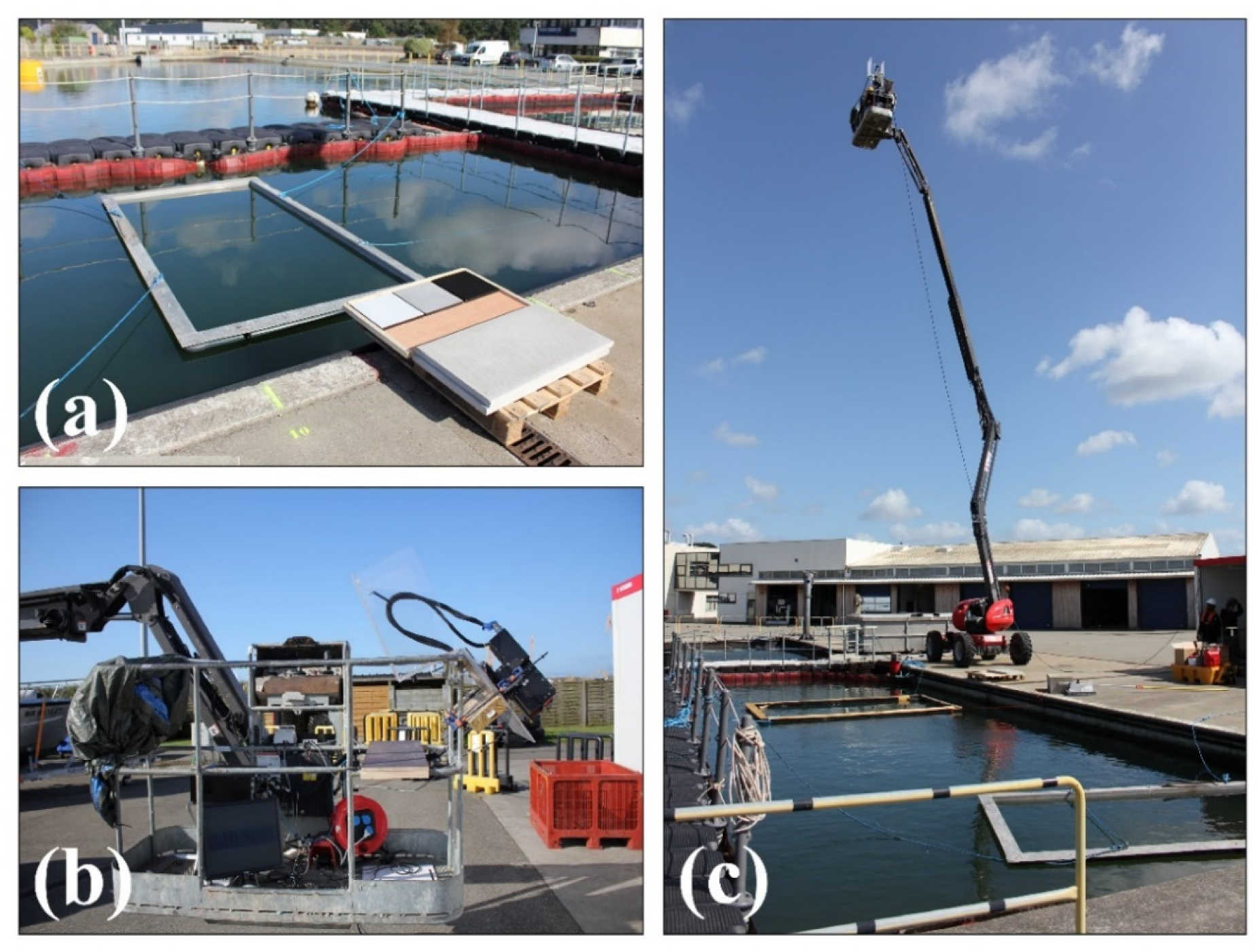
2.1. Ground Experiment of HNS
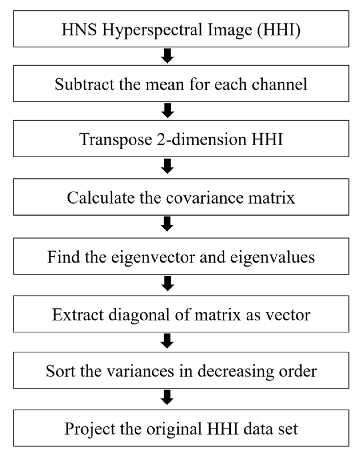
2.2. Dimension Reduction of HNS Hyperspectral Image
2.3. Hyperspectral Mixture Algorithm for HNS Detection
2.4. Hyperspectral Matching Algorithm
3. Results
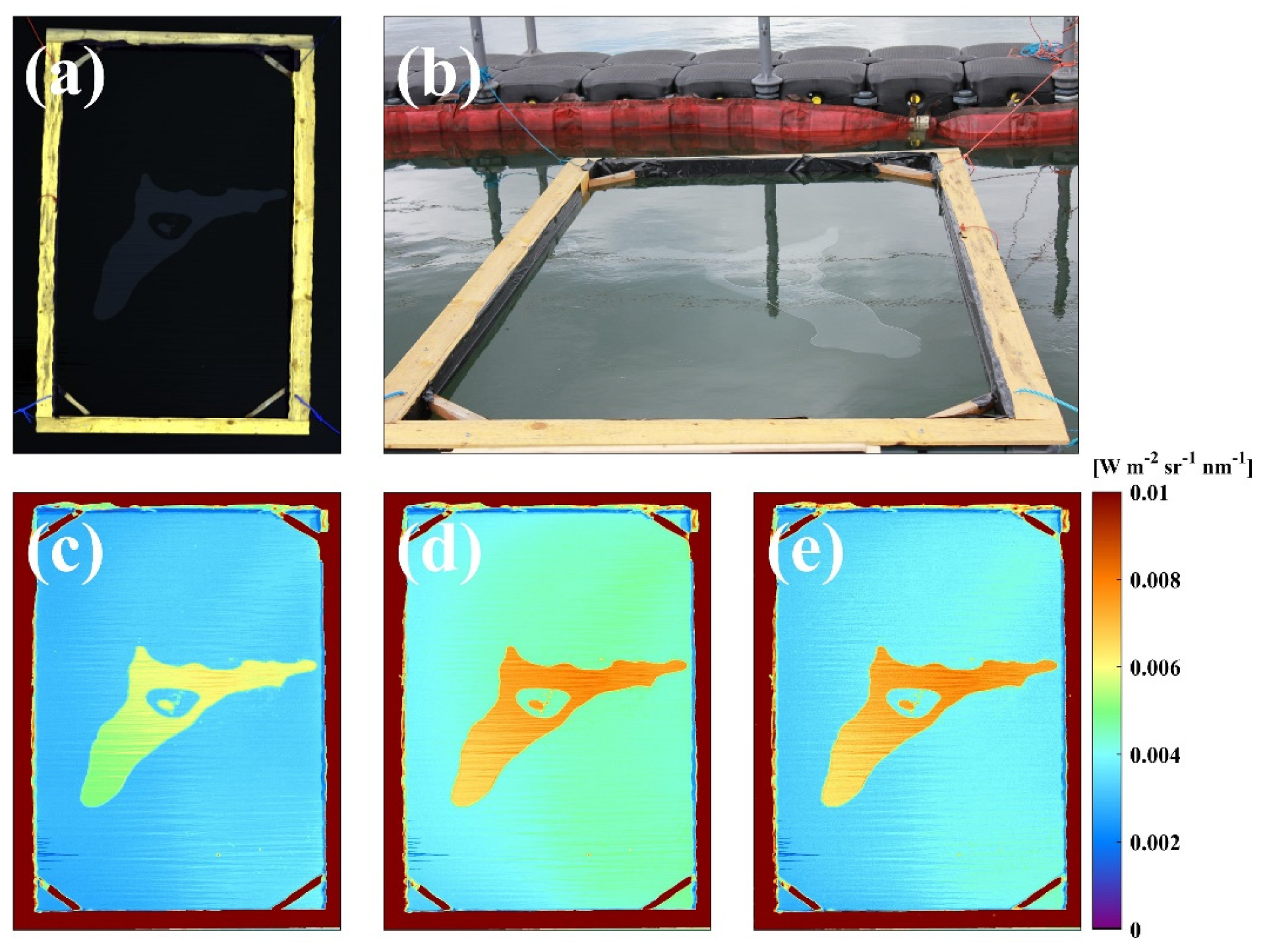
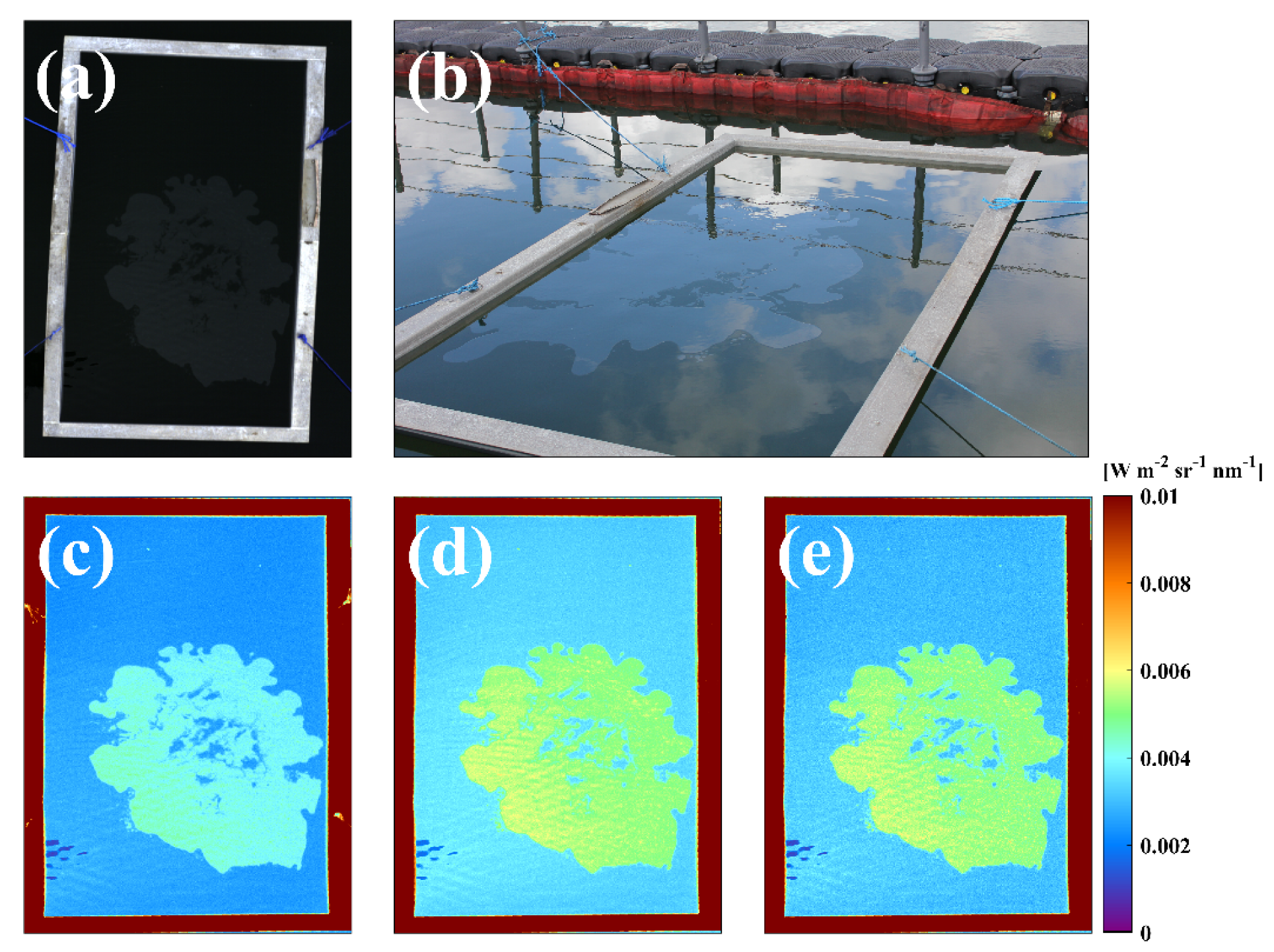
3.1. RGB Composite
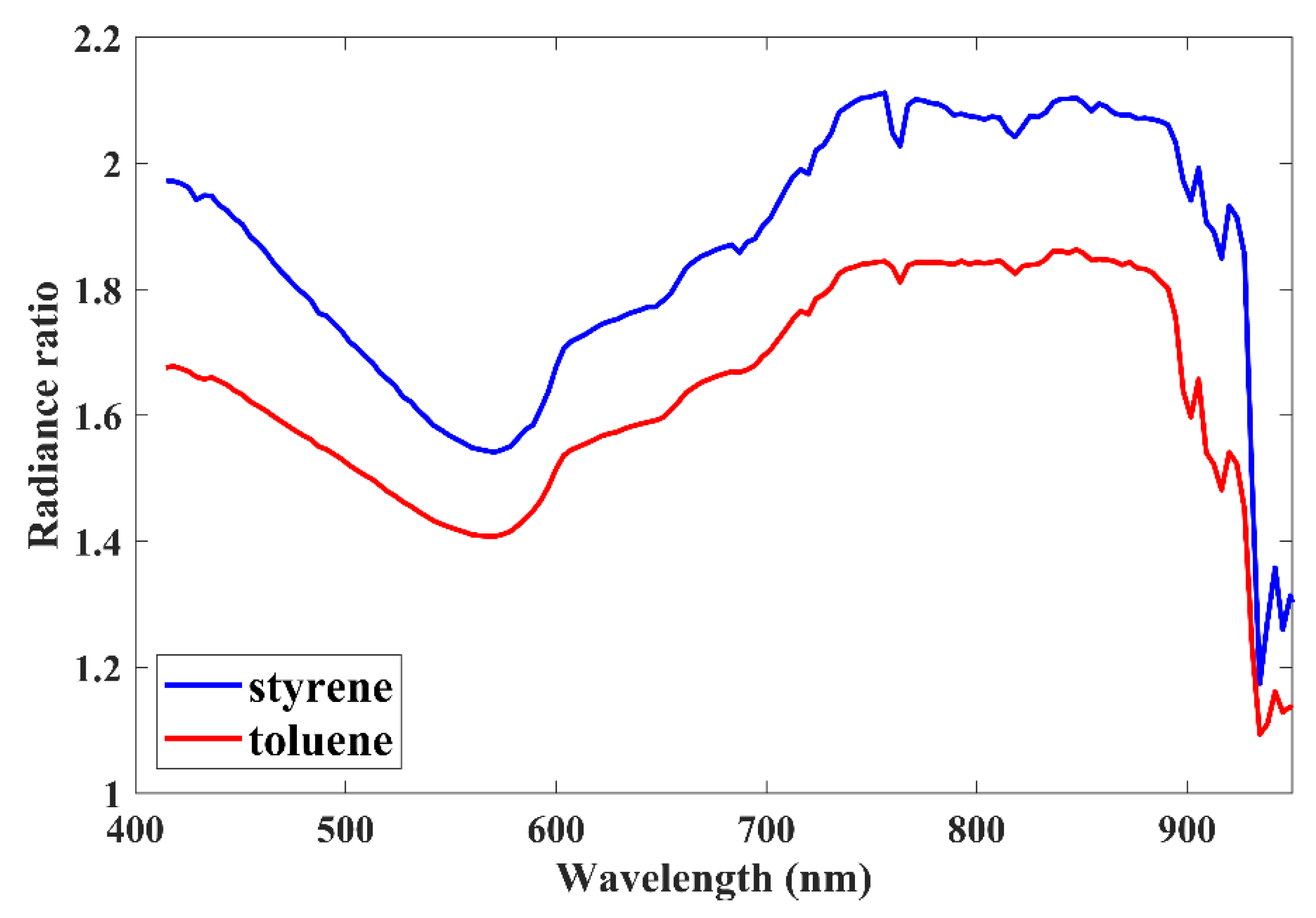
3.2. Characteristics of HNS Spectra at VNIR Wavelengths
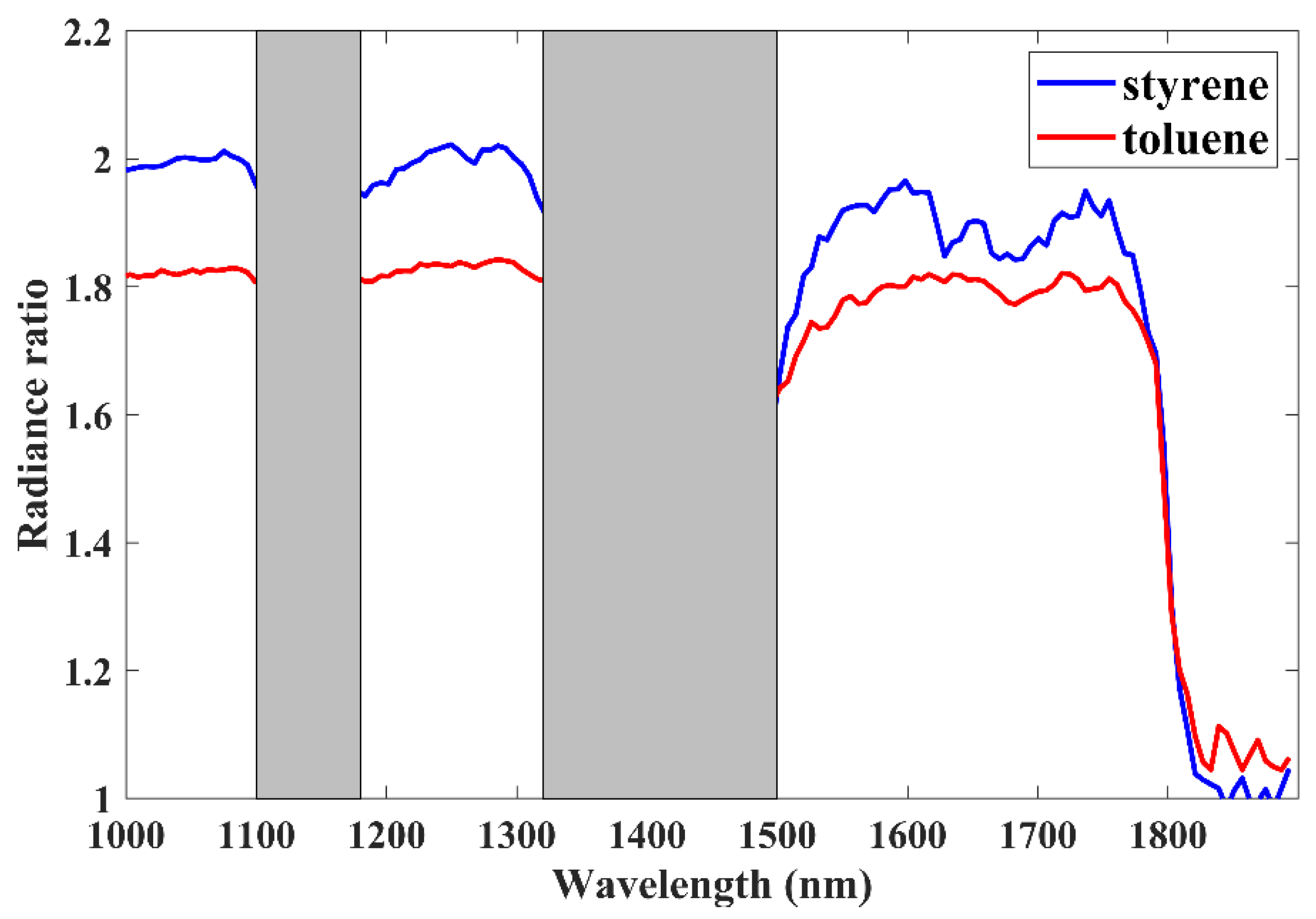
3.3. Characteristics of HNS Spectra at SWIR Wavelengths
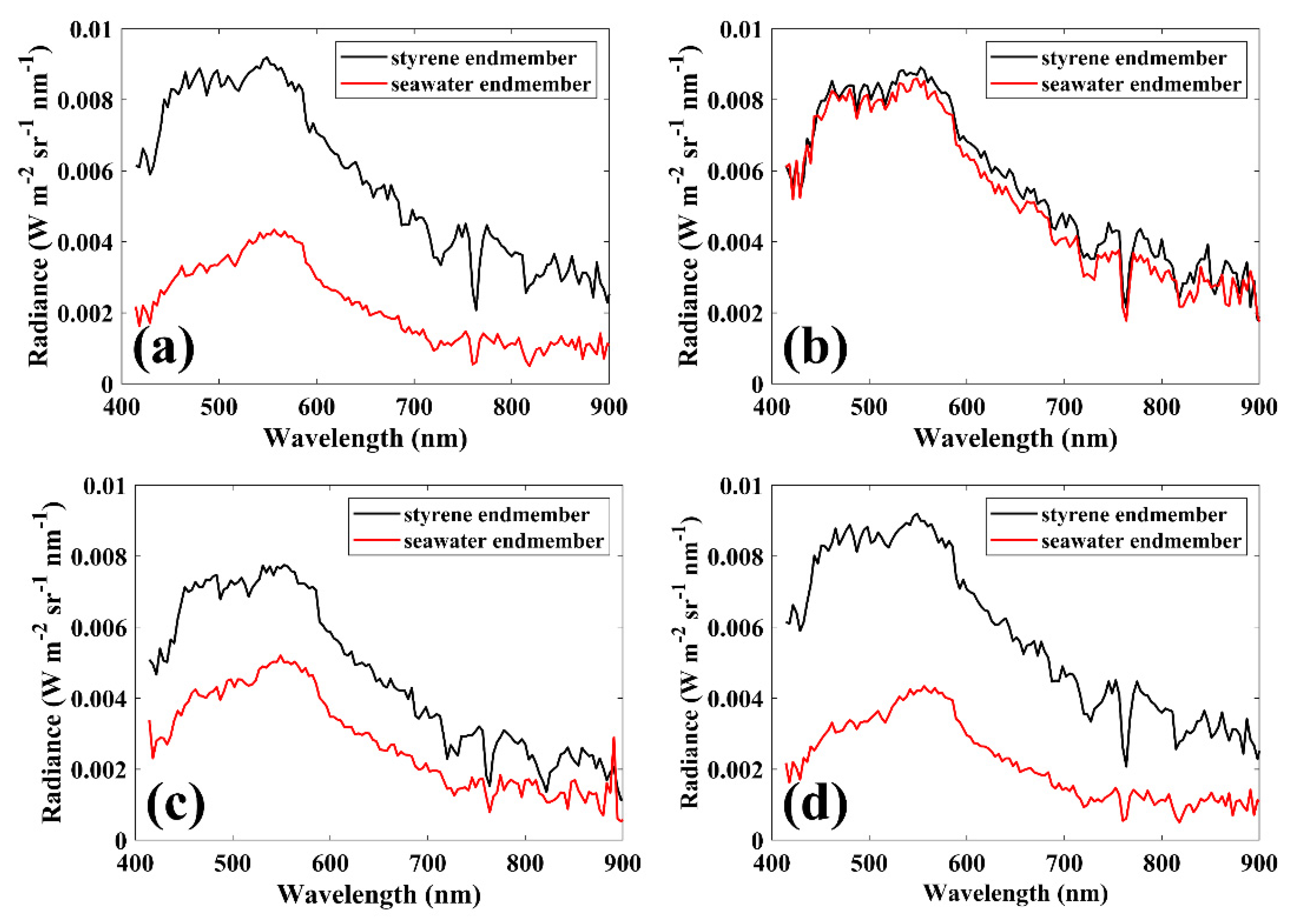
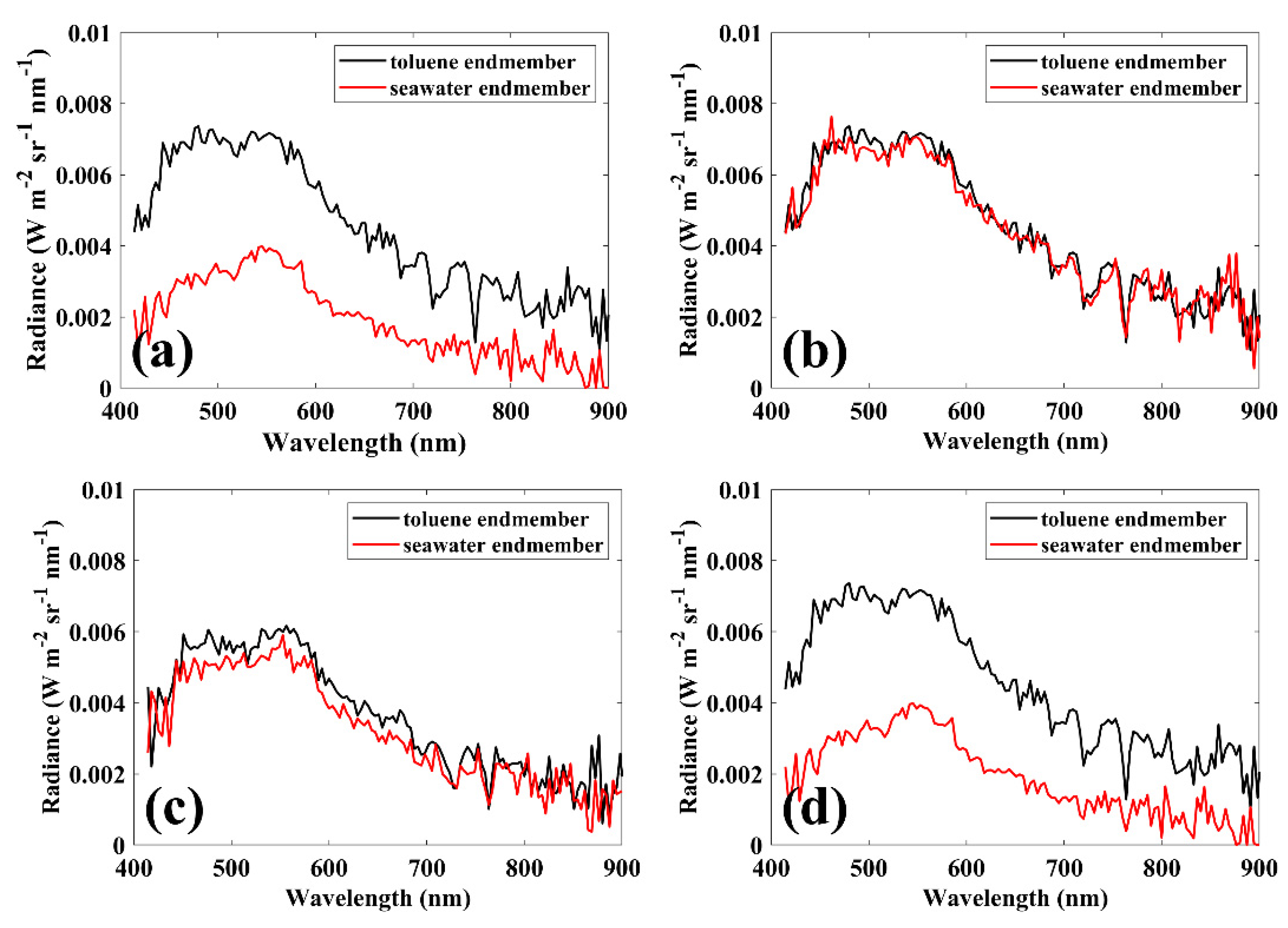
3.4. Comparison of Hyperspectral Mixture Algorithms
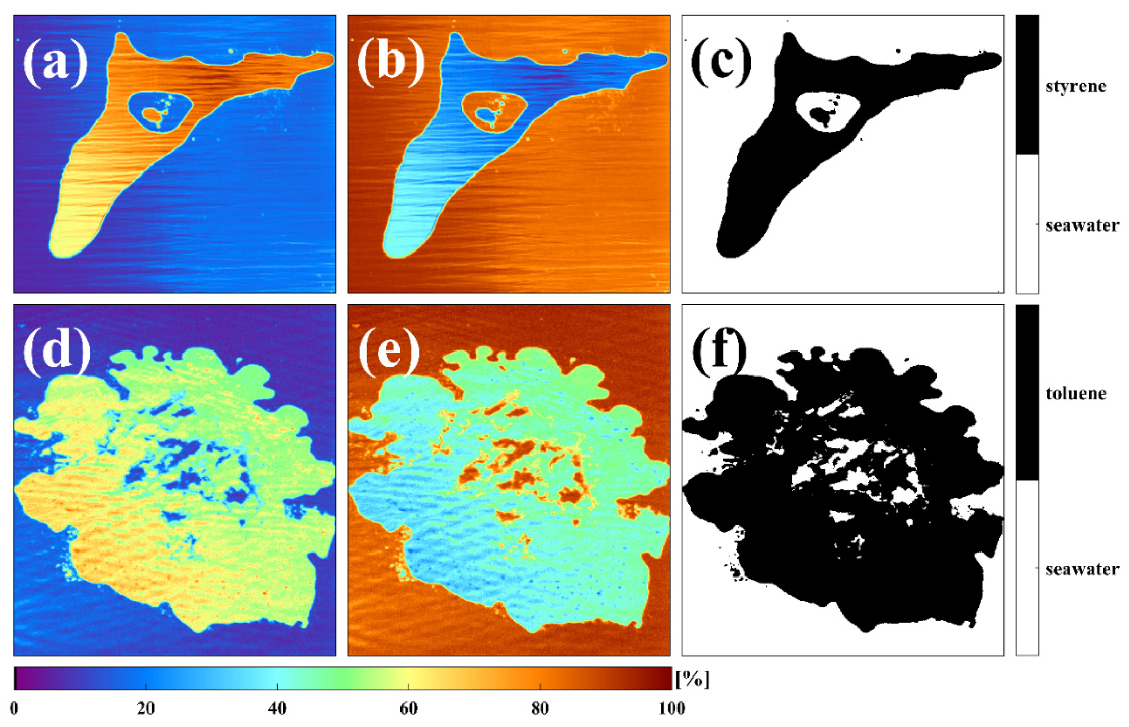
3.5. Abundance Fraction of HNS
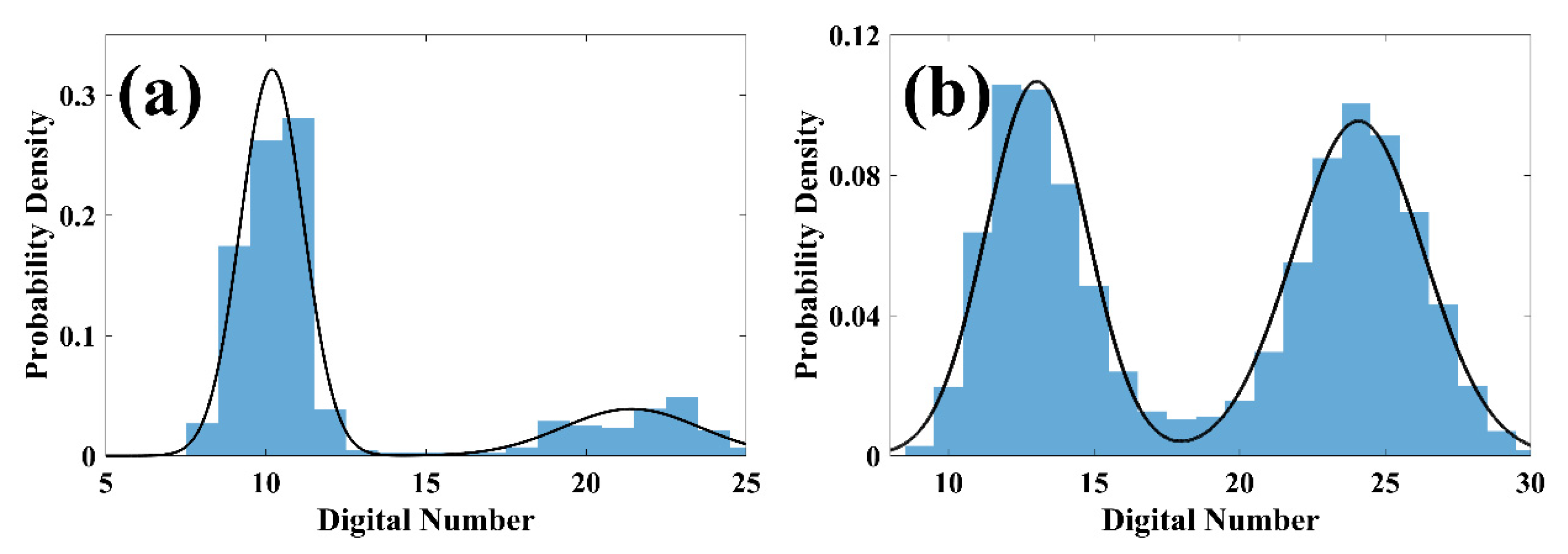
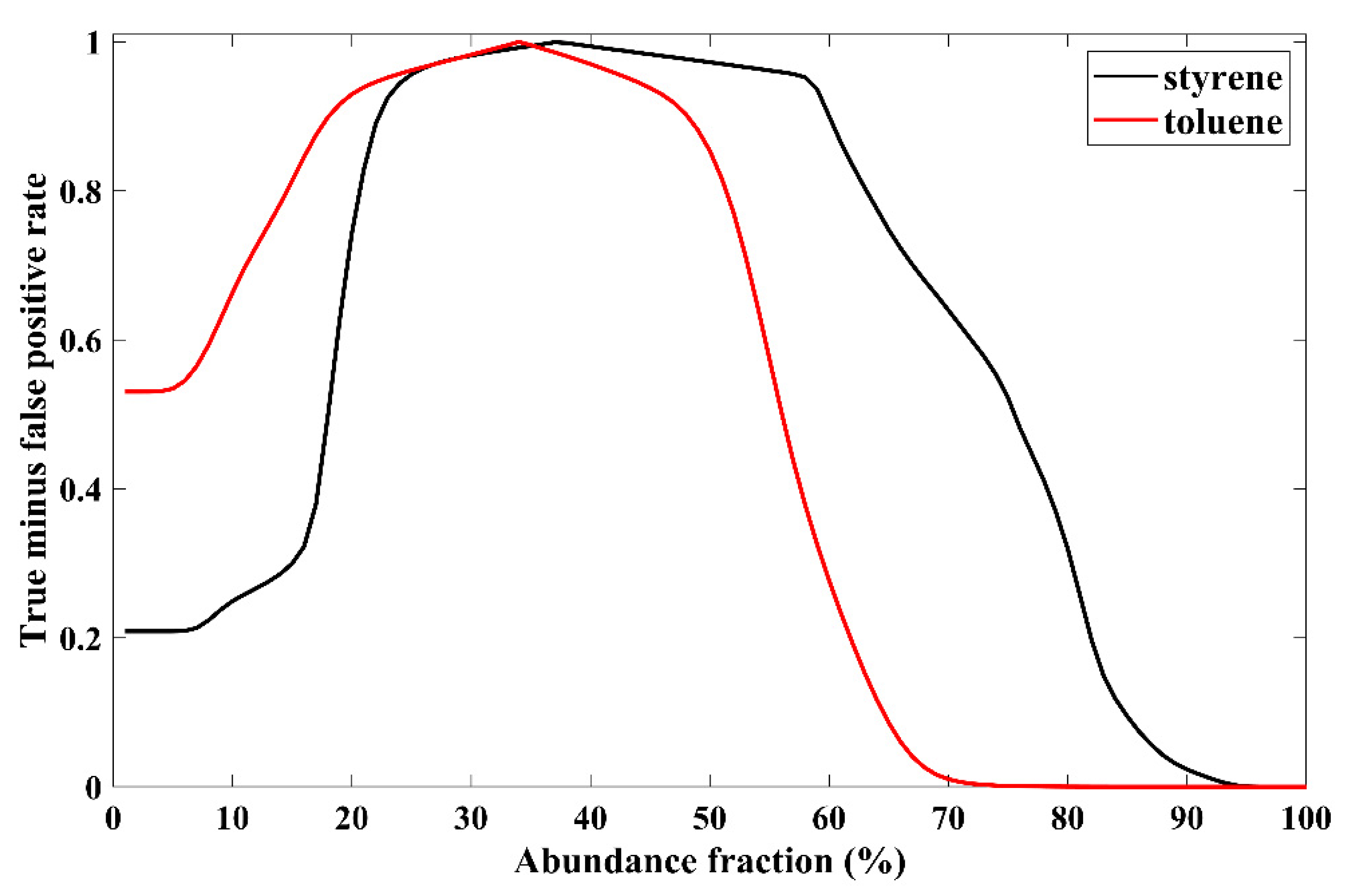
3.6. Determination of Optimal Threshold for HNS Detection
4. Discussion
5. Conclusions
Author Contributions
Funding
Institutional Review Board Statement
Informed Consent Statement
Data Availability Statement
Conflicts of Interest
References
- Chen, J.; Zhang, W.; Wan, Z.; Li, S.; Huang, T.; Fei, Y. Oil spills from global tankers: Status review and future governance. J. Clean. Prod. 2019, 227, 20–32. [Google Scholar] [CrossRef]
- Davenport, J. Oil and planktonic ecosystems. Philos. Trans. R. Soc. B 1982, 297, 369–384. [Google Scholar]
- Abbriano, R.M.; CARRANzA, M.M.; Hogle, S.L.; Levin, R.A.; Netburn, A.N.; Seto, K.L.; Franks, P.J. Deepwater Horizon oil spill: A review of the planktonic response. Oceanography 2011, 24, 294–301. [Google Scholar] [CrossRef]
- Felder, D.L.; Thoma, B.P.; Schmidt, W.E.; Sauvage, T.; Self-Krayesky, S.L.; Chistoserdov, A.; Fredericq, S. Seaweeds and decapod crustaceans on Gulf deep banks after the Macondo Oil Spill. Bioscience 2014, 64, 808–819. [Google Scholar] [CrossRef] [Green Version]
- Cheong, S.M. Fishing and tourism impacts in the aftermath of the Hebei-Spirit oil spill. J. Coast. Res. 2012, 28, 1648–1653. [Google Scholar] [CrossRef]
- Kim, T.S.; Park, K.A.; Li, X.; Lee, M.; Hong, S.; Lyu, S.J.; Nam, S. Detection of the Hebei Spirit oil spill on SAR imagery and its temporal evolution in a coastal region of the Yellow Sea. Adv. Space Res 2015, 56, 1079–1093. [Google Scholar] [CrossRef]
- Lee, M.S.; Park, K.A.; Lee, H.R.; Park, J.J.; Kang, C.K.; Lee, M. Detection and dispersion of thick and film-like oil spills in a coastal bay using satellite optical images. IEEE J. Sel. Top. Appl. Earth Obs. Remote Sens. 2016, 9, 5139–5150. [Google Scholar] [CrossRef]
- Loh, A.; Yim, U.H.; Ha, S.Y.; An, J.G.; Kim, M. Contamination and human health risk assessment of polycyclic aromatic hydrocarbons (PAHs) in oysters after the Wu Yi san oil spill in Korea. Arch. Environ. Contam. Toxicol. 2017, 73, 103–117. [Google Scholar] [CrossRef]
- Lee, M.; Jung, J.Y. Risk assessment and national measure plan for oil and HNS spill accidents near Korea. Mar. Pollut. Bull. 2013, 73, 339–344. [Google Scholar] [CrossRef]
- Harold, P.D.; De Souza, A.S.; Louchart, P.; Russell, D.; Brunt, H. Development of a risk-based prioritisation methodology to inform public health emergency planning and preparedness in case of accidental spill at sea of hazardous and noxious substances (HNS). Environ. Int. 2014, 72, 157–163. [Google Scholar] [CrossRef]
- Kim, Y.R.; Lee, M.; Jung, J.Y.; Kim, T.W.; Kim, D. Initial environmental risk assessment of hazardous and noxious substances (HNS) spill accidents to mitigate its damages. Mar. Pollut. Bull. 2019, 139, 205–213. [Google Scholar] [CrossRef] [PubMed]
- Li, Y.; Yu, H.; Wang, Z.Y.; Li, Y.; Pan, Q.Q.; Meng, S.J.; Guo, K.X. The forecasting and analysis of oil spill drift trajectory during the Sanchi collision accident, East China Sea. Ocean Eng. 2019, 187, 106231. [Google Scholar] [CrossRef]
- Chen, J.; Di, Z.; Shi, J.; Shu, Y.; Wan, Z.; Song, L.; Zhang, W. Marine oil spill pollution causes and governance: A case study of Sanchi tanker collision and explosion. J. Clean. Prod. 2020, 273, 122978. [Google Scholar] [CrossRef]
- Angelliaume, S.; Minchew, B.; Chataing, S.; Martineau, P.; Miegebielle, V. Multifrequency radar imagery and characterization of hazardous and noxious substances at sea. IEEE Trans. Geosci. Remote Sens. 2017, 55, 3051–3066. [Google Scholar] [CrossRef]
- Huang, H.; Liu, S.; Wang, C.; Xia, K.; Zhang, D.; Wang, H.; Li, X. On-site visualized classification of transparent hazards and noxious substances on a water surface by multispectral techniques. Appl. Opt. 2019, 58, 4458–4466. [Google Scholar] [CrossRef]
- Huang, H.; Wang, C.; Liu, S.; Sun, Z.; Zhang, D.; Liu, C.; Xu, R. Single spectral imagery and faster R-CNN to identify hazardous and noxious substances spills. Environ. Pollut. 2020, 258, 113688. [Google Scholar] [CrossRef]
- Zhan, S.; Wang, C.; Liu, S.; Xia, K.; Huang, H.; Li, X.; Xu, R. Floating Xylene Spill Segmentation from Ultraviolet Images via Target Enhancement. Remote Sens. 2019, 11, 1142. [Google Scholar] [CrossRef] [Green Version]
- Luo, G.; Chen, G.; Tian, L.; Qin, K.; Qian, S.E. Minimum noise fraction versus principal component analysis as a preprocessing step for hyperspectral imagery denoising. Can. J. Remote Sens. 2016, 42, 106–116. [Google Scholar] [CrossRef]
- Rodarmel, C.; Shan, J. Principal component analysis for hyperspectral image classification. Surv. Land Inf. Sci. 2002, 62, 115–122. [Google Scholar]
- Koonsanit, K.; Jaruskulchai, C.; Eiumnoh, A. Band selection for dimension reduction in hyper spectral image using integrated information gain and principal components analysis technique. Int. J. Mach. Learn. Comput. 2012, 2, 248. [Google Scholar] [CrossRef]
- Du, Q.; Fowler, J.E. Low-complexity principal component analysis for hyperspectral image compression. Int. J. High Perform. Comput. Appl. 2008, 22, 438–448. [Google Scholar] [CrossRef] [Green Version]
- Somers, B.; Asner, G.P.; Tits, L.; Coppin, P. Endmember variability in spectral mixture analysis: A review. Remote Sens. Environ. 2011, 115, 1603–1616. [Google Scholar] [CrossRef]
- Winter, M.E. N-FINDR: An Algorithm for Fast Autonomous Spectral End-Member Determination in Hyperspectral Data; Descour, M.R., Shen, S.S., Eds.; Imaging Spectrometry V.: Denver, CO, USA, 1999; Volume 3753, pp. 266–275. [Google Scholar]
- Chang, C.I.; Wu, C.C.; Tsai, C.T. Random N-finder (N-FINDR) endmember extraction algorithms for hyperspectral imagery. IEEE Trans. Image Process 2010, 20, 641–656. [Google Scholar] [CrossRef] [PubMed] [Green Version]
- Chang, C.I.; Plaza, A. A fast iterative algorithm for implementation of pixel purity index. IEEE Geosci Remote Sens Lett. 2006, 3, 63–67. [Google Scholar] [CrossRef]
- Wang, J.; Chang, C.I. Independent component analysis-based dimensionality reduction with applications in hyperspectral image analysis. IEEE Trans. Geosci. Remote Sens. 2006, 44, 1586–1600. [Google Scholar] [CrossRef]
- Dalla Mura, M.; Villa, A.; Benediktsson, J.A.; Chanussot, J.; Bruzzone, L. Classification of hyperspectral images by using extended morphological attribute profiles and independent component analysis. IEEE Geosci. Remote Sens. Lett. 2010, 8, 542–546. [Google Scholar] [CrossRef] [Green Version]
- Wang, J.; Chang, C.I. Applications of independent component analysis in endmember extraction and abundance quantification for hyperspectral imagery. IEEE Trans. Geosci. Remote Sens. 2006, 44, 2601–2616. [Google Scholar] [CrossRef]
- Nascimento, J.M.; Dias, J.M. Vertex component analysis: A fast algorithm to unmix hyperspectral data. IEEE Trans. Geosci. Remote Sens. 2005, 43, 898–910. [Google Scholar] [CrossRef] [Green Version]
- Lopez, S.; Horstrand, P.; Callico, G.M.; Lopez, J.F.; Sarmiento, R. A low-computational-complexity algorithm for hyperspectral endmember extraction: Modified vertex component analysis. IEEE Geosci. Remote Sens. Lett. 2011, 9, 502–506. [Google Scholar] [CrossRef]
- Heinz, D.C. Fully constrained least squares linear spectral mixture analysis method for material quantification in hyperspectral imagery. IEEE Trans. Geosci. Remote Sens. 2001, 39, 529–545. [Google Scholar] [CrossRef] [Green Version]
- Homayouni, S.; Roux, M. Hyperspectral image analysis for material mapping using spectral matching. In Proceedings of the ISPRS Congress, Istanbul, Turkey, 12–23 July 2004. [Google Scholar]
- Kumar, A.S.; Keerthi, V.; Manjunath, A.S.; van der Werff, H.; van der Meer, F. Hyperspectral image classification by a variable interval spectral average and spectral curve matching combined algorithm. Int. J. Appl. Earth Obs. Geoinf. 2010, 12, 261–269. [Google Scholar] [CrossRef]
- Sweet, J.N. The spectral similarity scale and its application to the classification of hyperspectral remote sensing data. In Proceedings of the Advances in Techniques for Analysis of Remotely Sensed Data, Greenbelt, MD, USA, 27–28 October 2003. [Google Scholar]
- Schwarz, J.; Staenz, K. Adaptive threshold for spectral matching of hyperspectral data. Can. J. Remote Sens. 2001, 27, 216–224. [Google Scholar] [CrossRef]
- Foucher, P.-Y.; Poutier, L.; Déliot, P.; Puckrin, E.; Chataing, S. Hazardous and Noxious Substance detection by hyperspectral imagery for marine pollution application. In Proceedings of the 2016 IEEE International Geoscience and Remote Sensing Symposium (IGARSS), Beijing, China, 10–15 July 2016; pp. 7694–7697. [Google Scholar]
- Park, J.J.; Kim, T.S.; Park, K.; Oh, S.; Lee, M.; Foucher, P.Y. Application of Spectral Mixture Analysis to Vessel Monitoring Using Airborne Hyperspectral Data. Remote Sens. 2020, 12, 2968. [Google Scholar] [CrossRef]
- Fingas, M. Weather Effects on Oil Spill Countermeasures. In Oil Spill Science and Technology; Gulf Professional Publishing: Oxford, UK, 2011; Volume 13, pp. 339–426. [Google Scholar]


| Characteristics | HySpex VNIR-1600 | HySpex SWIR-1800 |
|---|---|---|
| Acquisition process | Push broom | Push broom |
| Spatial pixels number | 1600 | 320 |
| Spectral pixels number | 160 | 256 |
| Field of view | 17° | 14° |
| Spectral domain | 400–1000 nm | 1000–2500 mm |
| Spectral width | 3.7 nm | 6 nm |
| Ground sample distance (row direction) | 2 mm | 6 mm |
| Ground sample distance (line direction) | 4 mm | 8 mm |
| HNS | Method | SDS | SCS | SSV | SAM |
|---|---|---|---|---|---|
| Styrene | N-FINDR | 0.9833 | 0.9853 | 0.9834 | 0.0395 |
| PPI | 0.7635 | 0.5860 | 0.8685 | 0.0491 | |
| ICA | 0.1522 | 0.8520 | 0.2123 | 0.0317 | |
| VCA | 0.9833 | 0.9853 | 0.9834 | 0.0395 | |
| Toluene | N-FINDR | 1.0173 | 0.6460 | 1.0771 | 0.1330 |
| PPI | 0.6087 | 0.0249 | 1.1495 | 0.0637 | |
| ICA | 0.5075 | 0.1936 | 0.9528 | 0.0715 | |
| VCA | 1.0173 | 0.6460 | 1.0771 | 0.1330 |
Publisher’s Note: MDPI stays neutral with regard to jurisdictional claims in published maps and institutional affiliations. |
© 2021 by the authors. Licensee MDPI, Basel, Switzerland. This article is an open access article distributed under the terms and conditions of the Creative Commons Attribution (CC BY) license (http://creativecommons.org/licenses/by/4.0/).
Share and Cite
Park, J.-J.; Park, K.-A.; Foucher, P.-Y.; Deliot, P.; Floch, S.L.; Kim, T.-S.; Oh, S.; Lee, M. Hazardous Noxious Substance Detection Based on Ground Experiment and Hyperspectral Remote Sensing. Remote Sens. 2021, 13, 318. https://0-doi-org.brum.beds.ac.uk/10.3390/rs13020318
Park J-J, Park K-A, Foucher P-Y, Deliot P, Floch SL, Kim T-S, Oh S, Lee M. Hazardous Noxious Substance Detection Based on Ground Experiment and Hyperspectral Remote Sensing. Remote Sensing. 2021; 13(2):318. https://0-doi-org.brum.beds.ac.uk/10.3390/rs13020318
Chicago/Turabian StylePark, Jae-Jin, Kyung-Ae Park, Pierre-Yves Foucher, Philippe Deliot, Stephane Le Floch, Tae-Sung Kim, Sangwoo Oh, and Moonjin Lee. 2021. "Hazardous Noxious Substance Detection Based on Ground Experiment and Hyperspectral Remote Sensing" Remote Sensing 13, no. 2: 318. https://0-doi-org.brum.beds.ac.uk/10.3390/rs13020318