Seasonal Variations of Daytime Land Surface Temperature and Their Underlying Drivers over Wuhan, China

1
Key Laboratory for Environment and Disaster Monitoring and Evaluation of Hubei, Innovation Academy for Precision Measurement Science and Technology, Chinese Academy of Sciences, Wuhan 430077, China
2
University of Chinese Academy of Sciences, Beijing 100049, China
*
Author to whom correspondence should be addressed.
Remote Sens. 2021, 13(2), 323; https://0-doi-org.brum.beds.ac.uk/10.3390/rs13020323
Submission received: 11 December 2020
/
Revised: 11 January 2021
/
Accepted: 14 January 2021
/
Published: 19 January 2021
(This article belongs to the Special Issue Feature Paper Special Issue: Large Spatial Scale Analysis and Intensive Data Use in Urban Social, Ecological, Economic, or Environmental System)
Abstract
:Rapid urbanization greatly alters land surface vegetation cover and heat distribution, leading to the development of the urban heat island (UHI) effect and seriously affecting the healthy development of cities and the comfort of living. As an indicator of urban health and livability, monitoring the distribution of land surface temperature (LST) and discovering its main impacting factors are receiving increasing attention in the effort to develop cities more sustainably. In this study, we analyzed the spatial distribution patterns of LST of the city of Wuhan, China, from 2013 to 2019. We detected hot and cold poles in four seasons through clustering and outlier analysis (based on Anselin local Moran’s I) of LST. Furthermore, we introduced the geographical detector model to quantify the impact of six physical and socio-economic factors, including the digital elevation model (DEM), index-based built-up index (IBI), modified normalized difference water index (MNDWI), normalized difference vegetation index (NDVI), population, and Gross Domestic Product (GDP) on the LST distribution of Wuhan. Finally, to identify the influence of land cover on temperature, the LST of croplands, woodlands, grasslands, and built-up areas was analyzed. The results showed that low temperatures are mainly distributed over water and woodland areas, followed by grasslands; high temperatures are mainly concentrated over built-up areas. The maximum temperature difference between land covers occurs in spring and summer, while this difference can be ignored in winter. MNDWI, IBI, and NDVI are the key driving factors of the thermal values change in Wuhan, especially of their interaction. We found that the temperature of water area and urban green space (woodlands and grasslands) tends to be 5.4 °C and 2.6 °C lower than that of built-up areas. Our research results can contribute to the urban planning and urban greening of Wuhan and promote the healthy and sustainable development of the city.

1. Introduction
Cities are gathering places for human activities and survival. With the development of cities and their population growth, urban management and planning have to confront an increasing number of issues, including significant urban climate effects. The urban heat island (UHI) is one of the most significant urban climate effects. It refers to the phenomenon that causes the atmospheric and surface temperatures in urban areas to be higher than in the surrounding rural areas [1,2]. The UHI effect has been linked to a series of negative impacts of cities, including the deterioration of air and water quality, indirect economic losses, reduced comfort, and increased mortality rate [3,4,5]. It has become a research hotspot in urban meteorology, urban planning, urban geography, and urban ecology [6].
UHI can be divided into “surface” and “air” (or “atmospheric”) UHIs based on the ways and heights that they are formed [7]. Air UHI refers to UHI effects in the canopy (CLHI) or boundary (BLHI) layer [8]. The CLHI is usually measured by in situ sensors mounted on fixed meteorological stations or traverses of vehicles [9,10,11,12], while more special platforms such as tall towers, radiosondes, and aircraft are needed to measure the BLHI [13]. The development and installation of these measurement devices are usually very time-consuming and expensive, and thus, they are only available in a few large cities worldwide to date [14]. Due to limited monitoring stations, the measured air UHIs usually fail to provide sufficient spatial details for urban land-use planning and climate change research [15,16,17,18]. In contrast, the surface UHI (SUHI), which represents the radiative temperature difference between urban and non-urban surfaces, is primarily measured by land surface temperature (LST) derived from thermal infrared (TIR) remote sensors [1]. TIR remote sensing can provide consistent and repeatable observations of the Earth’s surface, which offers the ability to study the urban thermal environment at various spatial (from local to global scales) and temporal (diurnal, seasonal, and inter-annual) scales with high accuracy and low cost [18,19,20]. SUHI has generally the opposite basic characteristics compared to atmospheric UHI: SUHI is most intense during the day (when the sun is shining) and in the summer season and shows more spatial and temporal variation than air UHI [2,21,22]. The challenge involves identifying spatial patterns and hotspots of LST in order to provide a scientific basis for better management of these heat poles in metropolitan cities. Geographical information system (GIS) mapping techniques can help to identify hotspots visually but not statistically [23]. The local Moran’s I index seems to be the most popularly used for hotspot or spatial cluster identification [24]. It has been successfully applied in hotspot identification of urban climate [25], economics [26], environmental monitoring [27], as well as in disease investigation [28].
At present, there are many effective remote sensors for estimating LST [29]. Indeed, since Rao [30] reported the first satellite-based observations of the SUHI phenomenon in the eastern United States in 1972, numerous studies of the UHI effect have been carried out using large-scale satellite LST datasets, such as the Advanced Very High Resolution Radiometer (AVHRR) data of the National Oceanic and Atmospheric Administration (NOAA) satellites [31,32] and the Moderate-Resolution Imaging Spectroradiometer (MODIS) data of the Terra/Aqua satellites [33,34]. However, the spatial resolution of these data is not sufficiently high to detect the LST variations of urban green spaces [29]. LST products with high spatial resolution are crucial for urban temperature mapping. For this reason, Landsat 8 Operational Land Imager and Thermal Infrared Sensor (Landsat 8 OLI/TIRS) data are widely used for the monitoring and retrieval of urban LST at the relatively fine spatial resolution of 30 m. For example, Guha [35] studied the relationship of LST with normalized difference vegetation index (NDVI) and normalized difference built-up index (NDBI) for the cities of Florence and Naples in Italy by using Landsat 8 data. Nurwanda [36] used Landsat 8 images to predict urban expansion and LST in Bogor City (Indonesia). These studies concerned the underlying structure of the city, especially the degree of weakening of the UHI by the allocation of urban green space [37,38,39,40].
The distribution of LST varies seasonally and is not only affected by land use/land cover but also by other driving factors, such as altitude, Gross Domestic Product (GDP) level, and population density [41,42,43]. However, in current studies, the driving forces of LST distribution are rarely explored comprehensively from the combined perspective of physical and socio-economic factors and interaction between driving factors [32,37,38,39,40]. Establishing a comprehensive driving factor system, determining the leading influencing factors of LST, and clarifying the action mechanisms of the driving factors have important scientific research significance and application value.
As a traditional industrial city in China and one of the national central cities planned for construction [44,45], Wuhan ranks among the highest in the country in terms of urbanization and problems related to the urban thermal environment [46,47]. Wuhan needs to face the inevitable challenge of how to best coordinate urban construction and development with environmental protection. At present, some studies have focused on the SUHI effect of Wuhan City and carried out the research on LST variations and its driving factors by using LST retrieval from TIR measures. For instance, Cao et al. [48] examined the effect impervious surfaces (IS) spatial patterns have on LST in Wuhan, China. They clarified the dynamic urbanization process of Wuhan and found that urbanization had a positive effect on LST but a negative effect on Enhanced Vegetation Index (EVI) [49]. Huang et al. [50] analyzed summer spatial temporal negative relationships of LST with NDVI, VF (vegetation fraction), and ISF (impervious surface fraction) and found a consistently strong negative relationship between LST and NDVI, as well as VF, and a positive relationship between LST and ISF. Shen et al. [46] generated high spatial resolution summer LST data for Wuhan for 1988–2013 and observed a decline in high temperature areas in the old city area and inter-annually stable relationships between distributions and land cover types. Huang et al. [47] proposed an indicator called Land Contribution Index (LCI) to better quantify the relationship between urban land-use types and UHI effect. Li et al. [51] obtained the land covers and LST maps of Wuhan from Landsat-5 images in 2000, 2002, 2005, and 2009, discussed the distribution of land-use/cover change and LST variation, and analyzed the correlation between population distribution and LST values in residential regions. Selecting Wuhan as a case study, Wang et al. [52] explored the climatic effect of landscape patterns and found that temperature contrast between surrounding landscape patches has a major influence on LST.
Although these studies focused on the effects of geographic environmental factors and human activity on LST variations, there is still a lack of studies that comprehensively compare factors and combinations of variables. In addition, most studies used correlation or regression analysis and focused little on quantitative analysis of multi-factors and their interactions. In comparison, the geodetector method can reveal the driving force behind a geographic phenomenon by detecting its spatial stratified heterogeneity. This method has been extensively used in the social sciences [53] and human health research [54] and is being popularized in natural [55] and environmental [56] sciences. The core assumption is that if a certain independent variable has a significant impact on a certain dependable variable, then there is relatively good agreement between the spatial distribution patterns of the independent and dependent variables [57]. Therefore, in this study, we conducted a multi-factor attribution analysis of LST variations in Wuhan using the geodetector method, with the seasonal spatial distribution of Wuhan’s LST derived from Landsat 8 OLI/TIRS.
The present research aims to analyze the seasonal spatial distribution of Wuhan’s LST by retrieving Landsat 8 images and identify the main driving factors affecting its cold and hot poles and their interactions. Furthermore, the differences in LST among cultivated lands, forest areas, grasslands and buil-up lands were quantitatively analyzed. The results of our study can provide a reference and scientific guidance to formulate urban development plans and effective mitigation of the UHI of Wuhan.
2. Study Area
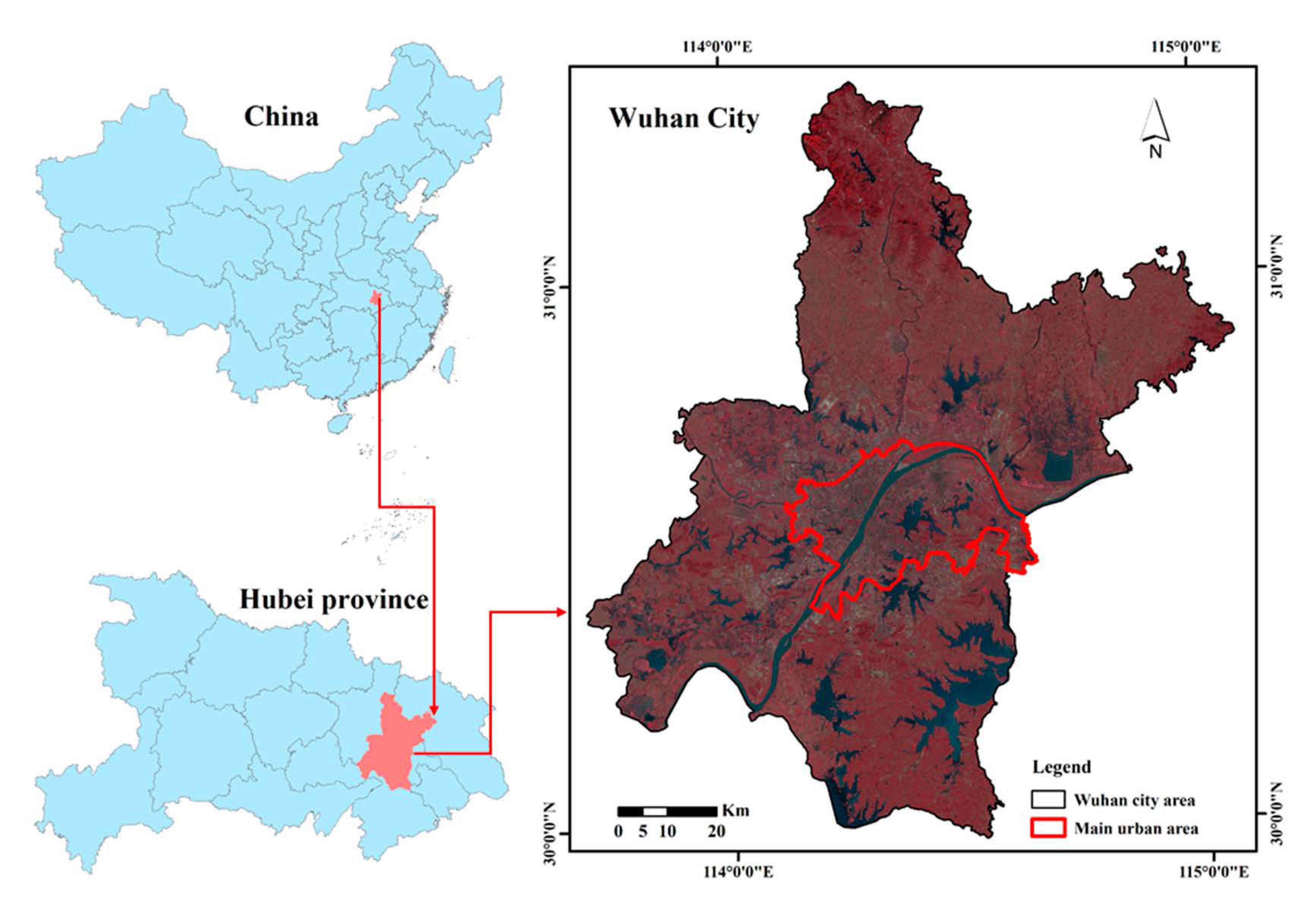
Wuhan City (113°41′–115°05′ E, 29°58′–31°22′ N) is the capital of Hubei Province and is located east of the Jianghan Plain and the middle reaches of the Yangtze River. It is a metropolitan city in the central China area, and it is also a significant transport interchange [42]. The Yangtze River and its largest tributary, the Hanjiang River, converge in the city. The rivers in the city are intertwined with lakes and ports. Wuhan is called “a city with 100 lakes”, as the water area accounts for almost a quarter of the city’s total area [58]. The study area belongs to a subtropical humid climate with an average annual temperature of 15.8–17.5 °C according to Köppen climate classification [42]. By the end of 2019, Wuhan had 13 districts with a total area of 8569.15 km2, a permanent resident population of about 11.21 million, and a regional GDP of 1.62 trillion yuan [59]. Seven adjacent central districts constitute its main urban area and account for 11.2% of the total area (Figure 1). Similar to Shanghai, Beijing, and Guangzhou, Wuhan has witnessed rapid urbanization in the past 30 years. Wuhan is recognized as one of the hottest “stove cities” in China [46,60,61]. Especially in summer, its daytime LST ranks at the top among China’s major cities, seriously affecting people’s living comfort. Therefore, it is urgent to monitor the LST in Wuhan and find its driving factors to improve its thermal comfort.
3. Data and Methods
3.1. LST Retrieval from Landsat Images
There are several algorithms for retrieving LST, including the radiative transfer equation (RTE) method [62], the single channel algorithm [63,64], and the split window algorithm [63,65]. However, these methods rely on near-real-time atmospheric profile data for when the satellites pass through the study area, which are hard to obtain. Therefore, similar to many other UHI studies [46,66], we employed a method in which only the NDVI and the Top of the Atmosphere (TOA) spectral radiance are needed. The parameter information in the header file can help acquire the TOA spectral radiance and reflectance of the Landsat-8 OLI/TIRS data. Adopting the conversion formula, the spectral radiance values of the Landsat thermal infrared bands were converted to at-sensor brightness temperatures under the assumption of uniform emissivity [67]:
where is the effective at-sensor brightness temperature in kelvin (K), is the TOA spectral radiance in W/(m2·sr·μm), and and are the calibration constants. For Landsat-8 TIRS, is 774.89 W/(m2·sr·μm) and is 1321.08 K for band 10 (http://landsat.usgs.gov/Landsat8_Using_Product.php).
The Tsensor values obtained above were referenced to a black body, which is quite different to the properties of real objects. Therefore, it was necessary to correct the spectral emissivity, and the LST based on satellite brightness temperature (Tsensor) was computed by the following equation [68]:
where is the LST in K; is the black body temperature, and also the satellite brightness temperature, in K; is the wavelength of the emitted radiance in meters; = 1.438 × 10⁻² mK; and is the surface emissivity.
For , water, (NDVI < 0) was assigned a value of 0.9925, urban impervious areas and bare soil (0 = <NDVI < 0.15) were assigned a value of 0.923 [69], and vegetation (NDVI > 0.727) was assigned a value of 0.986 [70]. Otherwise, there was a modeling relationship with the NDVI values through the following equation [71]:
NDVI was derived as follows:
where is the red band and is the near-infrared band.
Considering that the atmospheric environment is different between urban and rural areas [72,73], and in order to obtain accurate NDVI data, atmospheric correction is necessary to convert the TOA reflectance to surface reflectance [46,74]. In this study, we used the MODTRAN (Moderate Spectral Resolution Atmospheric Transmittance Algorighm And Computer Model) based FLAASH (Fast Line-of-sight Atmospheric Analysis of Spectral Hypercubes) model embedded in ENVI software for the atmospheric correction [46,75].
3.2. Landsat Images
We obtained all the available Landsat 8 OLI/TIRS images over Wuhan City during 2013–2019 with a maximum of 10% cloud cover (Table A1). All the Landsat 8 data were downloaded from the United State Geological Survey Earth Explorer website (http://earthexplorer.usgs.gov/); each set of Landsat data included three adjacent paths (path/row: 122/39, 123/38 and 123/39). The time of data acquisition was approximately 10:50 a.m. Greenwich Mean Time (GMT) in Wuhan.
3.3. Spatial Analysis of LST
3.3.1. Spatial Pattern analysis
Spatial autocorrelation means that the value of a variable at one location is correlated with the values of the same variable at its neighboring locations [76]. Spatial autocorrelation can be used to test whether the spatial distribution of LST presents clustering or discrete characteristics [76]. Cluster analysis can be used to find high and low temperature clusters, allowing study of the location and distribution characteristics of Wuhan’s hot and cold poles. Spatial autocorrelation is usually measured by Moran’s I, which includes the global and Anselin Local Moran’s I [27]. The Anselin Local Moran’s I calculates each sampling location to reveal its degree of spatial autocorrelation, and it is characterized by identifying spatial clusters of elements with high or low values, as well as identifying spatial outliers, which was described as follows [24]:
where is the value of the variable at location ; is the average value of with the sample number of n; is the value of the variable at all the other locations (where ); is the variance of variable ; and is a weight that can be defined as the inverse of the distance among locations and . The weight can also be determined using a distance band: samples within a distance band are given the same weight, while those outside the distance band are given the weight of 0.
Anselin Local Moran’s I statistic distinguishes between a statistically significant (0.05 level) cluster of high values (high–high clusters), cluster of low values (low–low clusters), outlier in which a high value is surrounded primarily by low values (high–low outliers), and outlier in which a low value is surrounded primarily by high values (low–high outliers) [23]. For this study, we employed the Anselin Local Moran’s I statistic to identify the spatial clusters and spatial outliers of Wuhan’s LST at the significance level of p < 0.05 in the four seasons of a year with the Cluster and Outlier Analysis tool in ArcMap 10.2 [77].
3.3.2. Geodetector Analysis
Geodetector is a new spatial statistical method mainly applied to identify the impact factors of spatial heterogeneity and the mechanisms through which they act [78,79,80]. It contains four detectors: a factor detector, risk detector, interaction detector, and ecological detector [57,81]. This study mainly used the factor detection and interaction detection of the geodetector to detect the driving mechanism of LST changes in Wuhan, and it quantified the impact of various factors on its change.
Factor detector detects the spatial heterogeneity of the dependent variable and the power of the determinant of the independent variables on the dependent variable. Factor detector is measured by q [78,80]:
where h = 1, …, L is the layer of independent variable X, and Nh and N are the number of sample units in layer h and the total region, respectively. and are the variance in the h layer and the variance in the region. SSW is the sum of the spatial variance of each layer, SST is the total variance of Y in the region, L is the layer number of factor X. The q lies in the range [0, 1], and q = 1 indicates that Y is completely determined by X, while q = 0 indicates there is no association between Y and X [57,80]. A larger q indicates a stronger explanatory power of the independent variable X to attribute Y.
The interaction detector is used to identify the interaction between influencing factors [57,82], that is, to evaluate the explanatory power of the combined (increased or decreased) and independent effects of the impact factors on LST. In the first step, the q of two impact factors on LST is calculated; then, the q of the interaction of the impact factors is calculated, and q (X1), q (X2), and q (X1 ∩ X2) are compared.
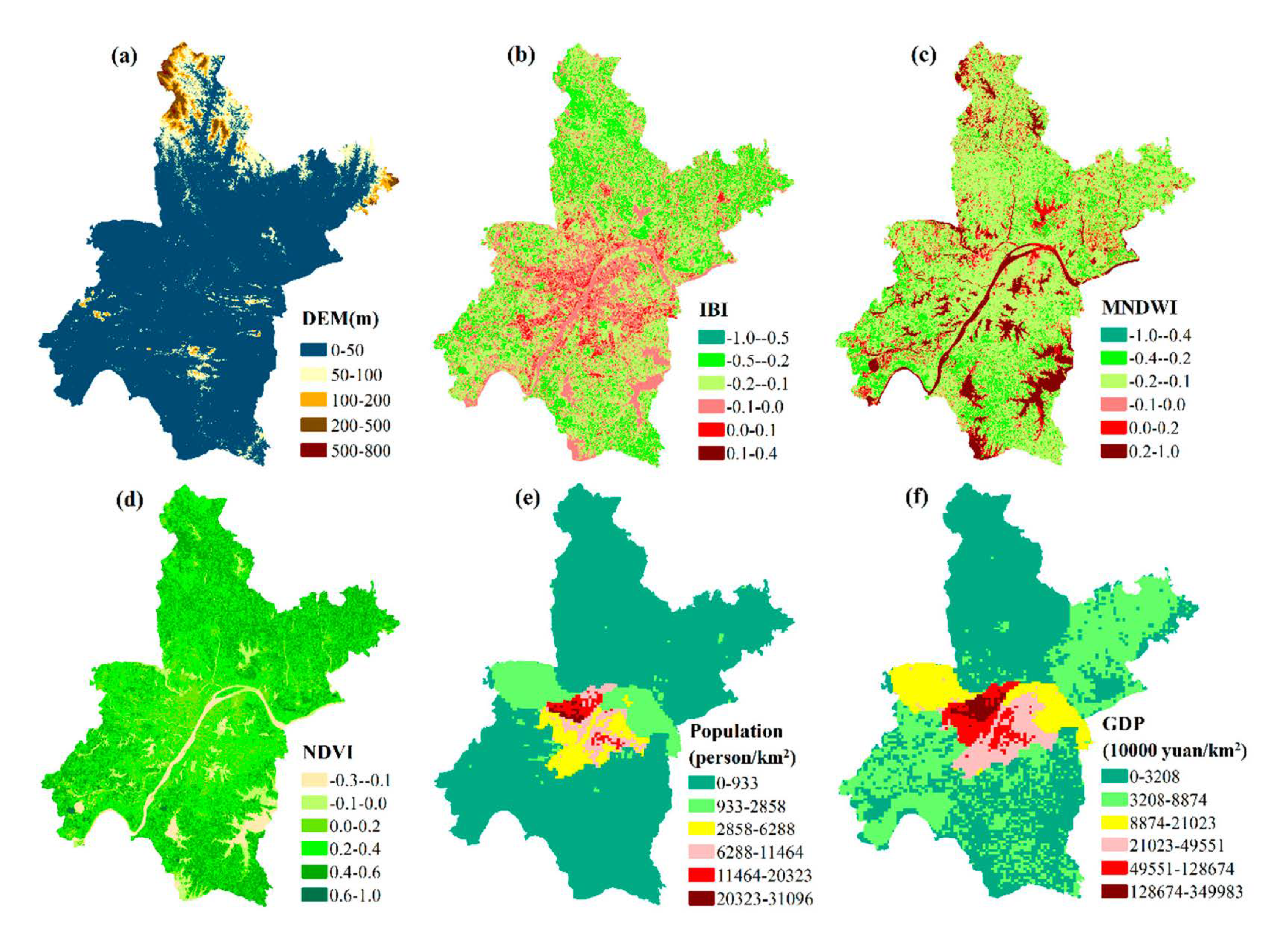
The 1 km grid GDP and population data of the study area in 2015 were obtained from the Resource and Environment Science and Data Center, Chinese Academy of Sciences (http://www.resdc.cn). For altitude, we used the Advanced Spaceborne Thermal Emission and Reflection Radiometer (ASTER) Global 30-m digital elevation model (DEM) V2 data. To characterize urban density, we used the index-based built-up index (IBI) proposed by Xu [83], which is defined as:
where is the medium infrared band and is the near-infrared band.
To estimate the presence of water and vegetation, the modified normalized difference water index (MNDWI) and NDVI (Equation (4)) were calculated separately. MNDWI was derived as follows [84]:
where is the green band and is the short-wave infrared band.
Figure 2 shows the spatial distribution of each LST driving factor.
3.3.3. Land-Cover Data
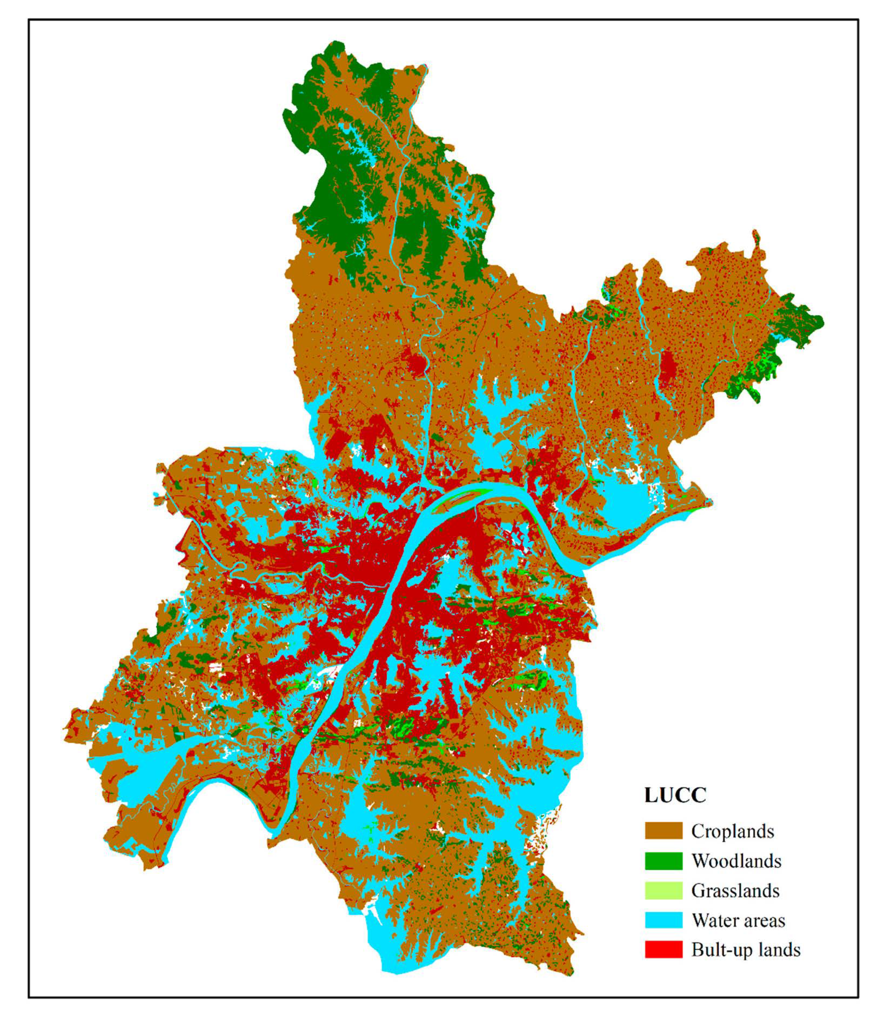
The land-use data of Wuhan in 2019 were obtained from databox.store (www.databox.store), which is a Chinese company dedicated to providing geographic big data products and services to government departments, universities, research institutes, enterprises, and other users. The Land-Use and Land-Cover Change (LUCC) classification system was established by the Institute of Geography of the Chinese Academy of Sciences, and it includes six primary types (croplands, woodlands, grasslands, water areas, built-up lands, and unused lands) and 25 secondary types. In the present study, we used five classes: croplands (includes paddy field and dry land) (52.6%), woodlands (includes forestland, shrubs, sparse woodland, orchards, etc.) (9.1%), grasslands (refers to all kinds of grasslands with a coverage of more than 5% of herbaceous plants) (0.8%), built-up lands (includes urban land, rural residential land, industrial and mining land, and traffic land) (16.5%) and water areas (include rivers, lakes, and beaches) (20.1%). A total of 99.1% of Wuhan city was analyzed (Figure 3). The remaining 0.9% were mainly unused areas. We extracted several statistical data from the LST of each land cover to detect the differences between different land covers, including minimum, maximum, mean, and standard deviation. In addition, kurtosis and skewness are also used to describe the spatial distribution of LST [29]. Skewness is a statistic to study the symmetry of data distribution [85]. By measuring the skewness coefficient, we can determine the asymmetry degree and direction of LST distribution. Kurtosis is a statistic that studies the steepness or smoothness of data distribution [85]. By measuring the kurtosis coefficient, we can determine whether the LST distribution is steeper or smoother than the normal distribution.
4. Results
4.1. Spatial Distribution of LST
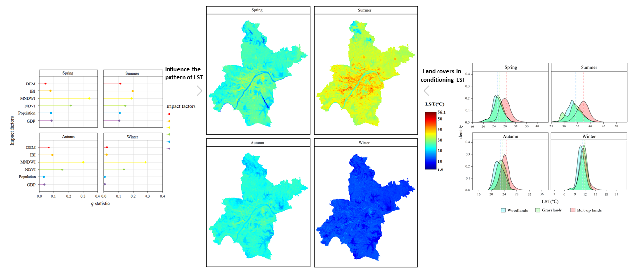
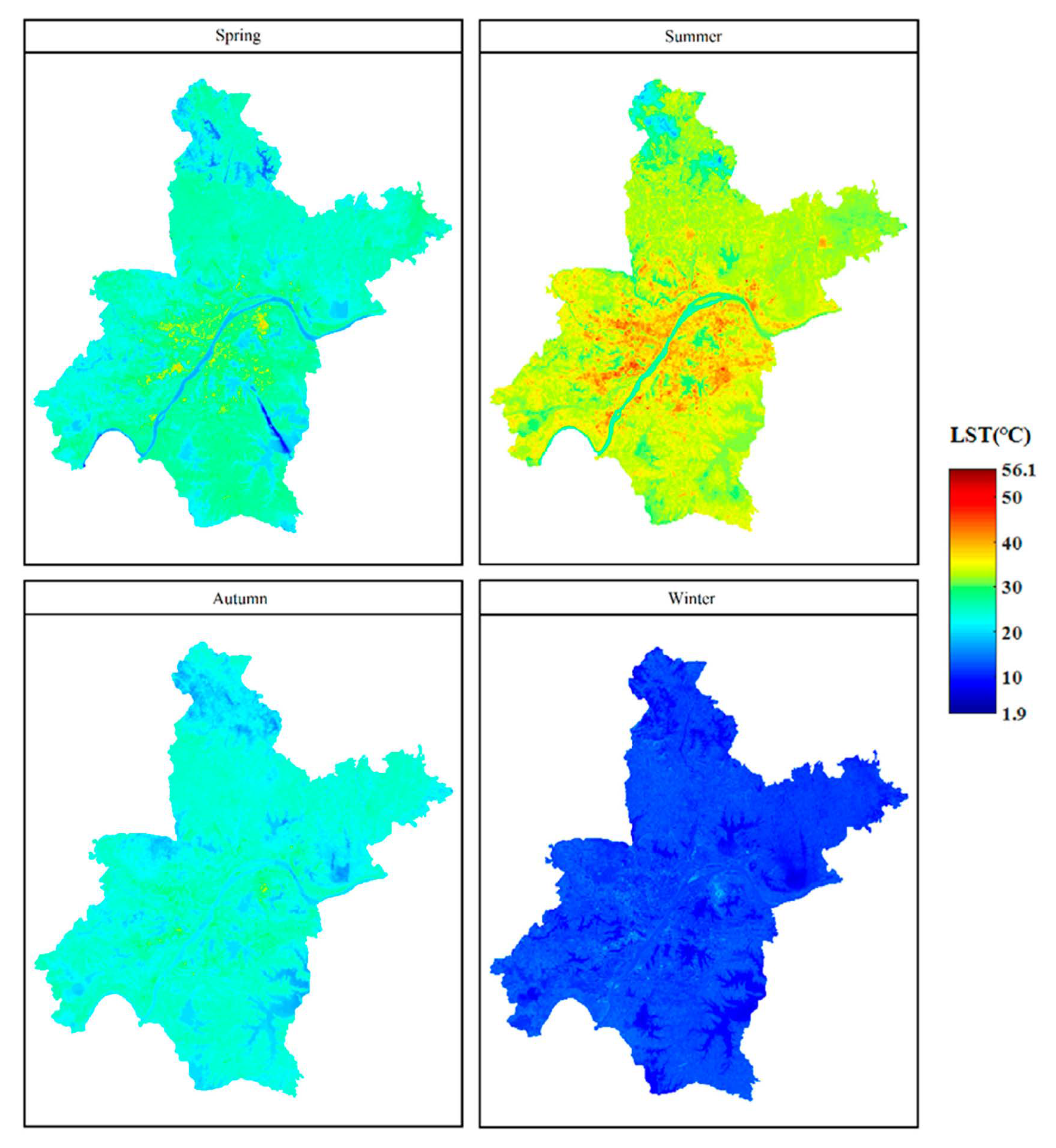
There are significant differences in the maximum, minimum, and average temperatures in Wuhan’s LST among the four seasons (Figure 4). The highest LST in spring is 43.8 °C, the average is 24.8 °C, and the lowest is 4.1 °C; the highest LST in summer is 56.1 °C, the average is 33.2 °C, and the lowest is 12.9 °C; the highest LST in autumn is 40.3 °C, the average is 23.1 °C, and the lowest is 13.2 °C; the highest LST in winter is 24.0 °C, the average is 11.6 °C, and the lowest is 1.9 °C. The standard deviation observed in spring (2.8 °C) and summer (3.2 °C) are higher than in autumn (1.9 °C) and winter (1.5 °C) (Table 1). A heat pole is shown in all four seasons in the main urban area, in the periphery and on the banks of the Yangtze River. In contrast, the coldest areas are found in the water area and forest zone.
4.2. Spatial Patterns of LST
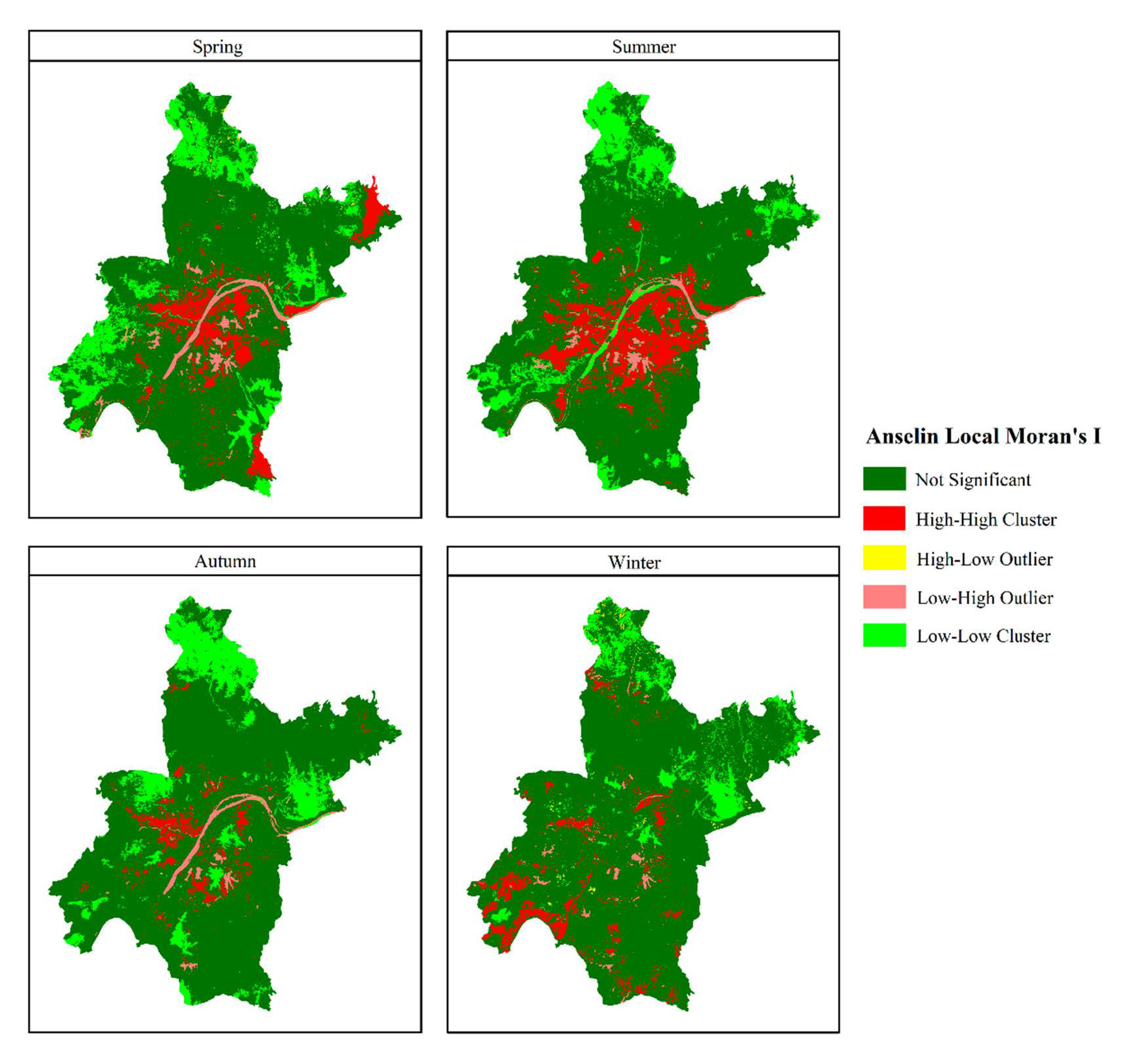
As shown in Figure 5, the spatial distribution of low and high temperature areas of Wuhan’s LST varied greatly in different seasons. The “high–high” cluster areas had the highest average LST in each season of the year, the highest in summer (38.4 °C), followed by spring (29.0 °C) and autumn (26.4 °C), and the lowest in winter (13.5 °C) (Table 2). These areas were larger in spring and summer, which was reflected in the proportion of area (8.40% and 11.88%, respectively), than in autumn and winter (3.47% and 5.27%, respectively). They were connected into a compact area with the Yangtze River as the symmetry axis, with a roughly symmetrical distribution, and they extended from the city center to the surrounding areas. The accumulation of high temperatures was more obvious in spring and summer. By comparing the LUCC map (Figure 3) of Wuhan City, it can be found that the “high–high” cluster areas of LST matched the spatial distribution of the built-up areas. The average LST of “low–low” cluster areas was the lowest in each season, the highest was in summer (29.0 °C), and the lowest was in winter (9.1 °C). The “low–low” cluster areas were mainly located in the major lakes, forest lands, and grasslands, indicating that the water area and green vegetation cover had a good cooling effect. Especially in the northeastern part of Wuhan, a large area of concentrated forest was a low-temperature region during the four study periods. Additionally, this area was also a high-altitude area in Wuhan. The “low–low” cluster areas was the largest in spring (15.10%) and the smallest in winter (8.02%). On the whole, Wuhan’s LST was more likely to cluster in summer, and the Anselin local Moran’s I showed that a total of 23.81% of the region showed significant spatial autocorrelation, which was the smallest in winter, only 13.29%.
4.3. Quantifying the Contribution of Impact Factors to LST
In this section, we analyzed the influence of six impact factors, including DEM, IBI, MNDWI, NDVI, population, and GDP (Figure 2) on the distribution of Wuhan’s LST.
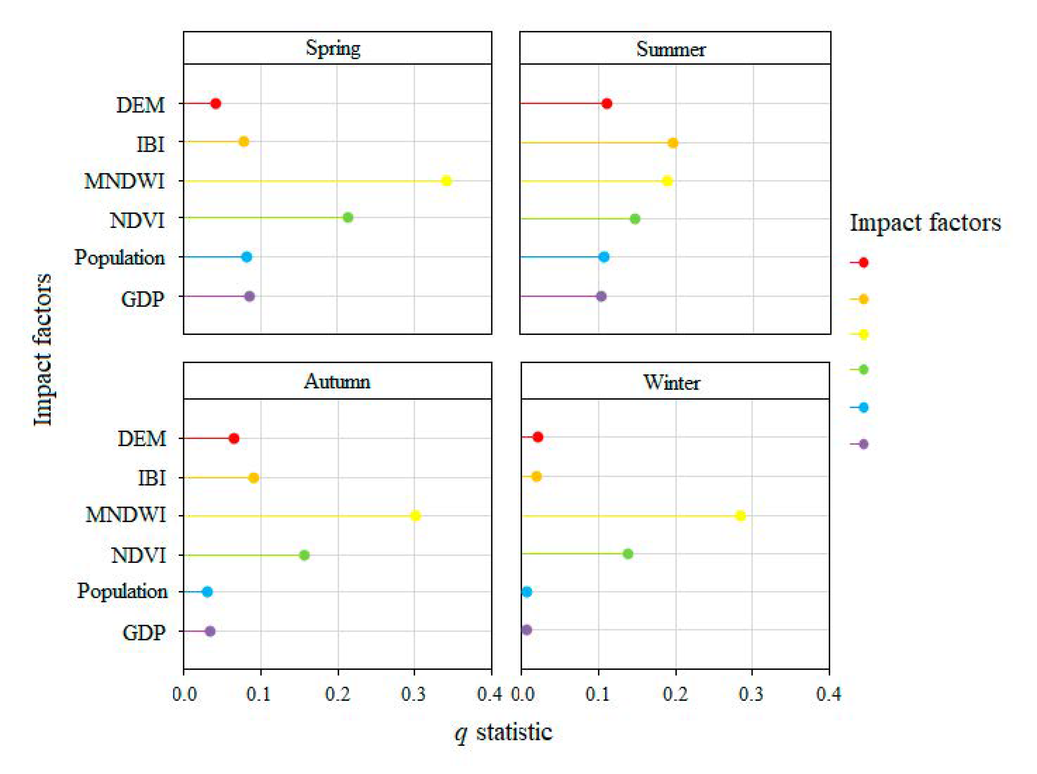
Firstly, the factor detector was used to determine the influence of each impact factor on LST change. It can be seen from Figure 6 that the q of all impact factors ranged from 0.008 to 0.342, but their impact on the four seasons was not completely consistent. In spring, MNDWI (0.342) > NDVI (0.215) > GDP (0.089) > Population (0.082) > IBI (0.079) > DEM (0.042); in summer, IBI (0.198) > MNDWI (0.190) > NDVI (0.148) > DEM (0.112) > GDP (0.111) > Population (0.109); in autumn, MNDWI (0.301) > NDVI (0.158) > IBI (0.092) > DEM (0.066) > GDP (0.039) > Population (0.031); in winter, MNDWI (0.284) > NDVI (0.138) > DEM (0.022) > IBI (0.020) > Population (0.009) > GDP (0.007). In general, MNDWI has the greatest impact on LST, which to a certain extent proves the importance of the water body in urban temperature regulation. This is followed by NDVI, which reflects that high-quality urban development cannot be separated from vegetation (including both natural and artificial vegetation). The third most important impact factor was IBI. Wuhan, as one of the largest cities in China, currently has a built-up area of 1419 km2, and urbanization is still increasing. The contribution of IBI to LST is expected to continue to increase.
The influence of each impact factor on the spatial distribution of LST was detected by using the interactive detector (Table 3). Overall, the interaction of any two impact factors on the change of LST was greater than one. For example, the q of the interaction between NDVI and MNDVI on LST change in spring was 0.470, which had the greatest influence on LST change, while the interaction between DEM and all socio-economic factors had a significantly greater influence on LST than DEM alone (0.420).
In terms of seasons, the interaction of NDVI and MNDWI was the largest (0.470) in spring, followed by the interaction between IBI and MNDWI (0.455). The interaction between IBI and MNDWI contributed the most to the variations of Wuhan’s LST in summer with the interaction of 0.439, which was followed by the interaction of IBI and NDVI (0.340). The interaction of IBI and MNDWI (0.411) was the largest in autumn, which was followed by the interaction between DEM and MNDWI (0.371). The interaction between GDP and MNDWI (0.310) was the largest in winter, which was followed by the interaction between MNDWI and IBI (0.308).
4.4. Land Cover Analysis of LST
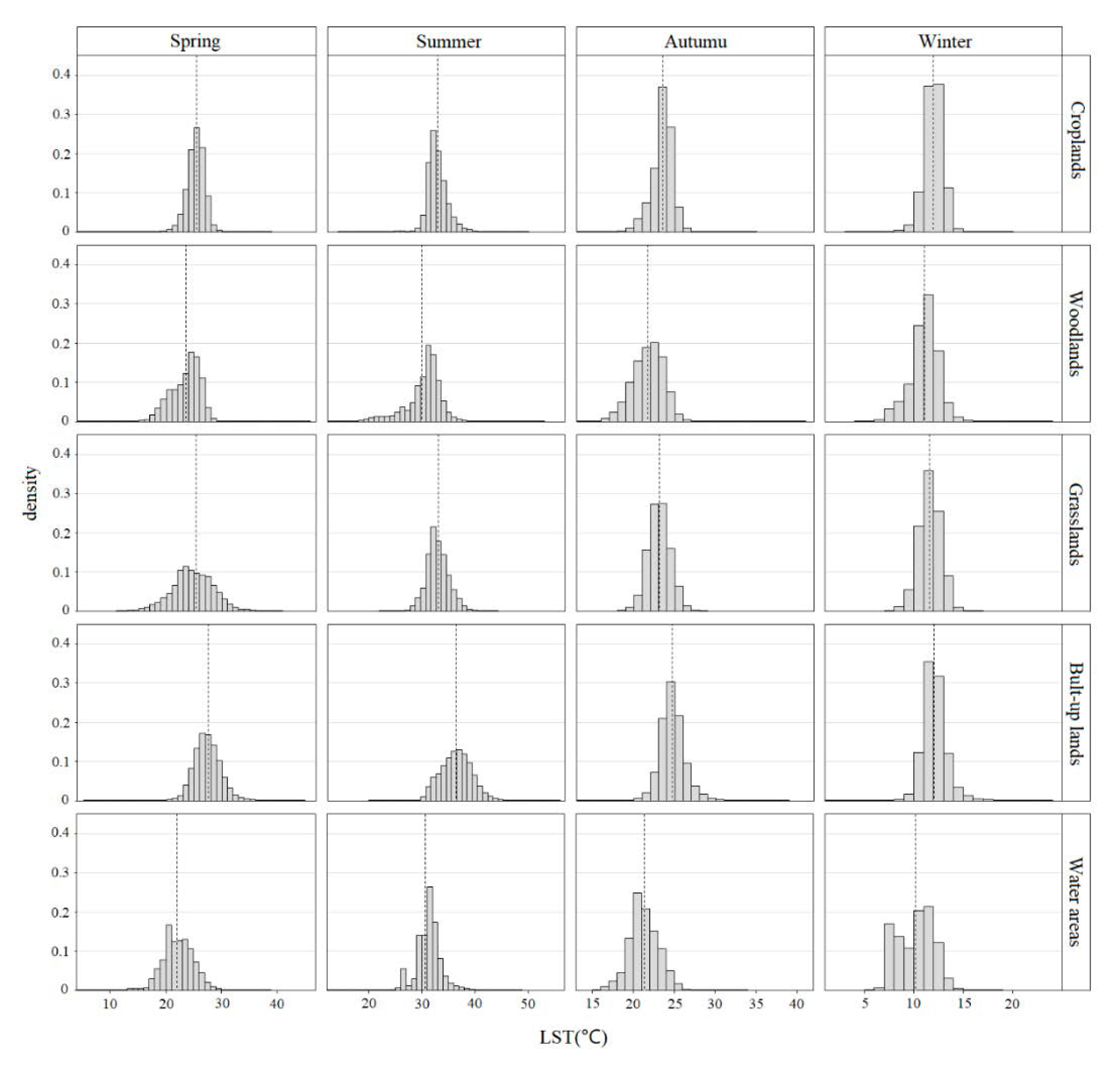
In this section, we quantified the difference of LST over the five land-cover types. Figure 7 shows the distribution of LST values for each land cover in the four seasons.
Among the five LUCC types, built-up land had the highest mean LST in the four seasons of the year (Table 4). This kind of land covers exhibited a broader thermal amplitude in the spring and summer, which is detectable in the standard deviation (1.6 °C and 1.2 °C, respectively), than in winter and autumn (2.5 °C and 3.0 °C, respectively). On an inter-annual scale, LST in the built-up area also presented the largest average thermal amplitude (24.8 °C), which was obtained by subtracting the mean LST in summer (36.9 °C) from the mean LST in winter (12.1 °C). The LST of cropland was lower than that of the built-up area in each season. The average LST of these two land covers was very close in winter, with only 0.1 °C difference, but the difference increased to 2.0 and 3.7 °C in spring and summer, respectively. Another characteristic of cropland was the high kurtosis in each season of the year, indicating that the LST distribution over croplands was more concentrated and had some outliers. The LST of most cropland pixels was below average, and the temperature difference was large. In addition, the long tail of the LST was on the right, which indicated that a small portion of the cropland pixels had a higher LST. This is probably due to the wide altitude range of croplands distribution (between 0 and 550 m) as well as different types of cultivated land and different farming systems, resulting in a large temperature difference among the agricultural lands.
The average LST of woodland in the four seasons was lower than that of several land covers analyzed before, forming a low-temperature zone in Wuhan. This gap was more obvious in spring and summer, especially in summer when it was 5.7 °C lower than the built-up area, resulting in the largest temperature difference recorded between different land covers in the same season. This is considered to be normal. Although the forest land in Wuhan is widely distributed from 0 to 800 m, it is mainly distributed in the high-altitude area northwest of Wuhan. Due to the influence of a vertical thermal gradient, the temperature of forest land could be expected to be lower than that of the built-up area and cropland. However, this difference began to decrease in autumn, and it was very small in winter (1.0 °C). On the inter-annual scale, the thermal amplitude of woodland was the smallest (20.1 °C). The mean LST of grassland was higher than that of woodland and less than that of construction land in four seasons. It was very close to agricultural land, but it exhibited a lower temperature, which showed the cooling function of grassland to a certain extent. In addition, the thermal amplitude of grassland in each season was very small, which can be seen from the standard deviation. The last land-use type analyzed was water area, which was another low-temperature area in Wuhan City. The performance of the average LST of the water area in the four seasons was very similar to that of woodland. It had the lowest temperature in all seasons, creating the smallest average LST record for a year (10.2 °C). However, the Yangtze River in winter was an exception. The average temperature of the Yangtze River was higher than that of all land covers, including the water area, with a temperature of 12.4 °C. A possible explanation for this phenomenon is the fact that the Yangtze River’s waterway is busy with water transportation and high anthropogenic heat emission, which increase the temperature of the Yangtze River.
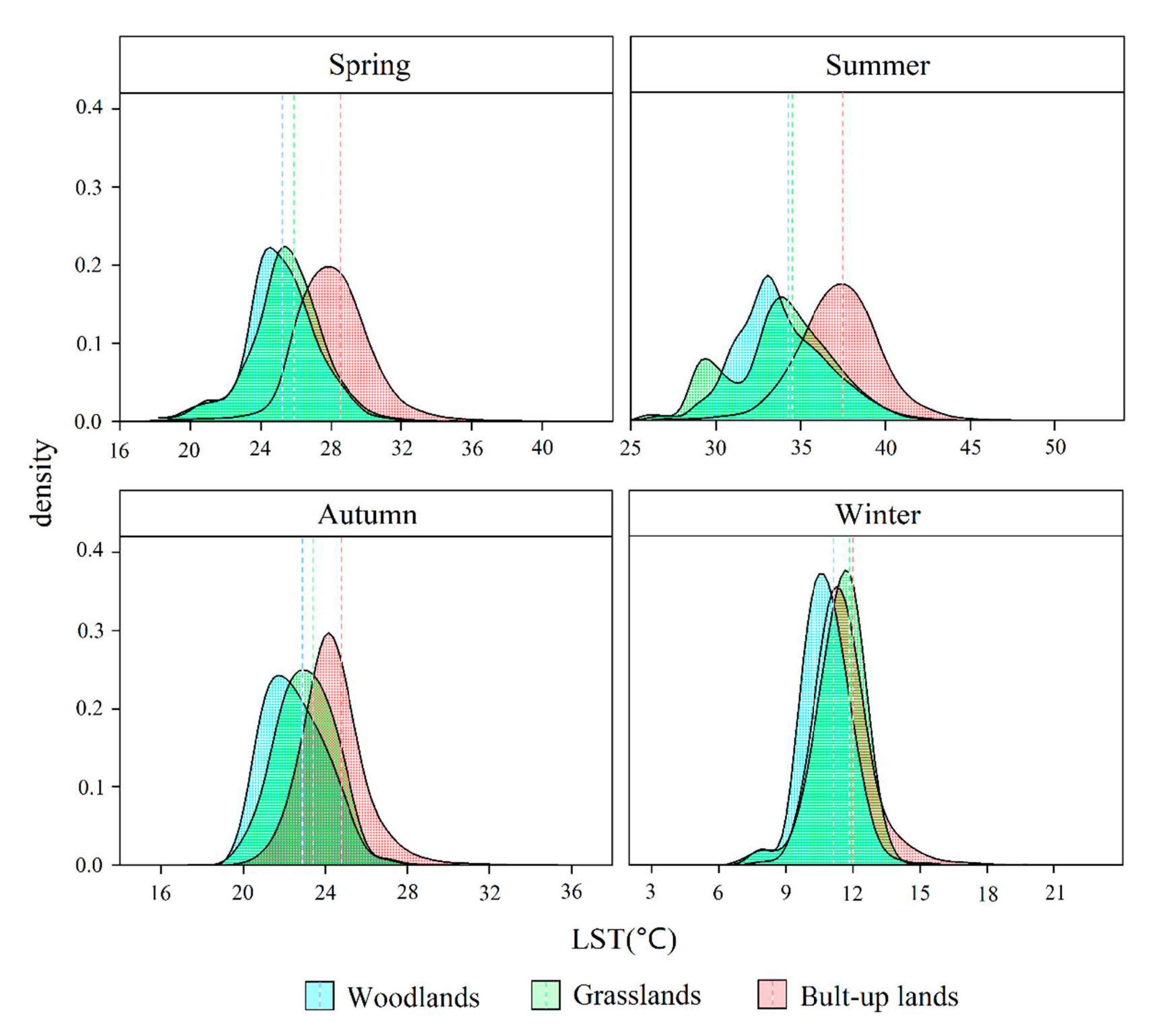
Although there are thermal differences between different land covers, because they are not at the same altitude, their comparison is not straightforward. To better compare the thermal differences between the urban green spaces (woodlands and grasslands) and the built-up areas in Wuhan, and to eliminate the errors caused by the vertical decline rate of temperature, we further analyzed the seasonal performance of LST for woodlands, grasslands and built-up lands in the main urban area within the altitude range of 0–100 m (Figure 8). In addition, we excluded agricultural land because to emphasize the thermal differences within cities and the potential impact that such thermal differences may have on urban settlements and living conditions. In addition, water bodies were also removed to highlight the cooling effect of green spaces in Wuhan.
The LST of the urban green spaces (woodland and grassland) in Wuhan City tended to be 2.6 °C lower than that in the built-up area in spring and summer (Table 5). The mean difference between the three land covers was very small in winter (0.8 °C). This means that the region was generally colder in winter within the same altitude range, with an average temperature of 11.8 °C. However, this phenomenon ended in the spring when the temperature began to gradually warm up. The thermal amplitude of built-up land increased higher than that of woodland and grassland (27.1 °C). Although the mean LST of woodland and grassland decreased, the difference between woodland and built-up land increased to 2.9 °C. In summer, the mean LST of woodland and grassland decreased further, and the difference between woodland and built-up land increased further. At this time, we detected the maximum temperature difference of 3.4 °C. In autumn, the thermal amplitude of each land-cover type began to fall, and the average difference between woodland and built-up land also shrank to 1.9 °C.
5. Discussion
5.1. Effects of Impact Factors on LST
In this study, we used Landsat-8 OLI/TIRS data to examine the relationship of DEM, IBI, MNDWI, NDVI, population, and GDP with LST in Wuhan, China. The results from factor detector show that all these factors have effects on LST, although the explanatory power of each factor is different. Due to the complexity of geographic processes, controlling factors often do not act independently but instead act collectively [57,86]. The extent to which the effects of controlling factors can be combined remains an unresolved issue [86]. This study examined the interaction between any two of the factors affecting LST distribution using the geodetector method to determine its pattern. The results show that the interactions between MNDWI, IBI, and NDVI were the main factors influencing the variations of Wuhan’s LST in each season. Previous studies [43,87,88,89] have confirmed that physical factors such as water and vegetation play an important role in mitigating SUHI by using the remote sensing index (MNDWI and NDVI). Similarly, there is no high-temperature agglomeration in Wuhan’s water area and forest land. Peng et al. [90] found that DEM shows a great impact on LST in Western Sichuan Plateau, China. However, our results show that DEM has no significant impact on Wuhan’s LST. This difference could be due to the dominant topography of the Western Sichuan Plateau being mountainous land, most having altitudes of 2000–3000 m, accounting for 83.4% of the total area, while Wuhan is mainly located in a plain area, and the area with elevation below 100 m accounts for 95.5% of its total area.
With the acceleration of urbanization and industrialization, the influence of socio-economic factors on LST variations is becoming more and more important [88,91]. The impact of socio-economic factors, such as anthropologic heat releases and build-up intensity, on the spatial distribution pattern of SUHI were confirmed in China’s 32 major cities [92]. On the whole, among the three social factors (IBI, Population, GDP) used in this study, IBI has the strongest explanatory power to LST, whether it is the single explanatory power or interactive explanatory power with other factors. Previous studies also showed the importance of IBI (or normalized difference built-up index (NDBI)) on LST variations [89,91]. The larger the area of urban construction land, the higher the NDBI and LST [93]. The enhancement of LST by impervious surface (IS) was more pronounced in individual cities than in urban agglomerations [94]. Therefore, high-temperature areas in Wuhan are mainly concentrated in built-up land. A remarkable feature of the winter thermal environment in Wuhan was the high temperature in a section of the Yangtze River (Figure 4), which is similar to the results by Guo et al. [95] for the winter surface thermal environment of Nanjing City (China). This phenomenon cannot be explained by the large specific heat capacity of the water bodies alone, because there were no high temperatures in Hanjiang River, Donghu Lake, and Tangxun Lake. Considering its important economic and shipping status, the Yangtze River has become the world’s largest comprehensive transportation channel, with railways, expressways, pipelines, and ultra-high voltage power transmission lines [96]. Wuhan port is one of the 28 major ports in China and the largest public terminal operator in Hubei Province. There are a large number of industrial and transportation facilities along the river [97]. Many studies have also shown that anthropogenic heat emissions are deteriorating the thermal environment of water bodies [98,99,100]. Therefore, the thermal environmental anomalies in the Wuhan section of the Yangtze River in winter may be caused by anthropogenic thermal emissions related to transport heat release. In a word, the three main impact factors and other impact factors jointly affect the spatial aggregation and distribution pattern of Wuhan’s LST.
Our study also shows that the driving factors of LST pattern in Wuhan are complex and seasonal, not static [47], because the most powerful explanatory factors are different in each season (see Section 4.3). Similar results were found in Shenzhen City (China) by Peng et al. [43], who showed that the most important factors affecting spatial heterogeneity of LST in summer and transition seasons were NDBI and NDVI, respectively, while in winter, they were construction land percentage and NDVI.
5.2. The Role of Different Land Covers in Conditioning LST
With respect to the combined analysis of the different land covers and LST estimated by Landsat, several cities, such as Shenyang, China [101] and Kuala Lumpur metropolitan area, Malaysia [102], show patterns similar to Wuhan, with built-up land displaying the highest temperatures among the land-use types, the lowest being recorded in the water area. As we all know, the specific heat capacity of water is higher than that of soil, which has a certain regulating effect on temperature. As an inland city, the large water area is a distinctive feature of Wuhan. It could be found from Table 4 that the LST of water areas in Wuhan city tends to be 5.4 °C lower than that in the built-up area in spring and summer, reflecting that the water area plays an important role in cooling Wuhan. Le et al. [103] used Landsat 8 images to study the relationship between urban landscape patterns and the thermal environment in Longquan, which is a national forest city in China. They found that the lowest temperature area was in forest land, which was slightly different from our research results. This may be because the forest land of Longquan occupies 87.4% of the land area, while the water area only accounts for 0.8%; in contrast, the water area of Wuhan accounts for 20.1% of the total area.
The temperature difference between built-up area and forest land is more significant in spring and summer, while they reach a minimum in winter, which was consistent with the results of the Rotterdam (Netherlands) metropolitan area obtained by Van Hove [104] and the results provided by Lemus-Canovas [29] for Barcelona (Spain). This is mainly because in spring and summer, the daytime is long, the height of the sun at noon is high, and the ground receives more solar radiation, which increases the heating differences between different types of surfaces of the city. The SUHI study in Italian metropolitan cities also found that the daytime SUHI increased significantly in summer, especially in inland cities, by increasing the size of areas with low tree cover densities in the metropolitan core (or decreasing areas with low tree cover densities outside the metropolitan core), further increasing its intensity when the impervious density grew [33]. This study revealed that urban green space has a clear impact on the reduction of the urban thermal environment and can effectively mitigate the UHI [66]. For three megacities in Southeast Asia—Bangkok (Thailand), Jakarta (Indonesia) and Manila (Philippines)—the average LST of the green space was found to be about 3 °C lower than that of the impervious surface, which is close to our results (2.6 °C), highlighting its role in weakening the UHI [6]. Here, an increase in NDVI tends to mean a gradual decrease in UHI [105]. In contrast, the city of Jaipur (India) has witnessed considerable growth in built-up area at the expense of greener patches over the last decade; as a result, its UHI has been strengthened and extended to new regions [106].
6. Conclusions
This study examined the spatial variation of daytime land surface temperatures in Wuhan from 2013 to 2019 and the driving factors affecting its cold and hot poles. The main results are as follows:
- (1)
- LST in Wuhan shows spatial aggregations, with high temperature areas mainly distributed in the built-up areas and low temperature areas mainly distributed in water and woodland areas. In summer, during the study period, the average temperature difference among different land covers rose to 6.2 °C, while in winter, this average difference dropped to 1.9 °C.
- (2)
- Physical and socio-economic factors and their interactions were responsible for the patterns of LST differences in Wuhan. Among them, MNDWI, IBI, and NDVI, relating to the distribution of water areas, built-up, and green spaces and their interactions, were the main factors affecting temperature differences.
- (3)
- In spring and summer, the water area and urban green spaces (woodland and grassland) registered an LST of up to 5.4 °C and 2.6 °C lower than the built-up lands, respectively. From this perspective, water area and urban green spaces plays an extraordinary role in improving the thermal comfort of the city and preventing the occurrence of high temperature heat stress.
This study can help to objectively manage the relationship between urban built-up areas, green spaces, and forest lands in urban planning and construction.
Author Contributions
Conceptualization, L.C.; Data curation, L.C., X.C. and X.W.; Formal analysis, L.C.; Funding acquisition, X.W., C.Y. and X.L.; Methodology, X.C. and X.W.; Software, L.C., C.Y. and X.L.; Supervision, X.W. and X.C.; Writing—original draft, L.C.; Writing—review and editing, L.C., X.W., X.L. and C.Y. All authors have read and agreed to the published version of the manuscript.
Funding
This work was supported by the National Natural Science Foundation of China (Grant No. 41571202, 41801100); the China Postdoctoral Science Foundation (2020M682526).
Institutional Review Board Statement
Not applicable.
Informed Consent Statement
Not applicable.
Acknowledgments
In this section, you can acknowledge any support given which is not covered by the author contribution or funding sections. This may include administrative and technical support, or donations in kind (e.g., materials used for experiments).
Conflicts of Interest
The authors declare no conflict of interest.
Appendix A

Table A1.
Landsat-8 OLI/TIRS images of the Wuhan City used in this study (Section 3.2).
Table A1.
Landsat-8 OLI/TIRS images of the Wuhan City used in this study (Section 3.2).
| Sensor | Date | Remarks | |||
|---|---|---|---|---|---|
| 2013-04-26 | 2013-05-12 | 2015-03-31 | 2016-03-01 | Spring | |
| 2016-04-18 | 2018-04-08 | ||||
| 2013-06-13 | 2013-07-31 | 2015-08-22 | 2016-06-05 | Summer | |
| 2016-07-23 | 2017-07-26 | 2019-06-14 | 2019-08-01 | ||
| Landsat-8 | 2019-08-17 | ||||
| 2013-09-17 | 2013-11-04 | 2013-11-20 | 2014-10-06 | Autumn | |
| 2014-10-22 | 2015-10-25 | 2015-11-26 | 2017-10-30 | ||
| 2018-09-15 | 2018-11-02 | 2019-10-20 | 2019-11-05 | ||
| 2013-12-06 | 2014-01-23 | 2017-02-16 | 2017-12-17 | Winter | |
| 2019-12-07 |
References
- Voogt, J.A.; Oke, T.R. Thermal remote sensing of urban climates. Remote Sens. Environ. 2003, 86, 370–384. [Google Scholar] [CrossRef]
- Ferguson, B.; Fisher, K.; Golden, J.; Hair, L.; Haselbach, L.; Hitchcock, D.; Kaloush, K.; Pomerantz, M.; Tran, N.; Waye, D. Reducing Urban Heat Islands: Compendium of Strategies; EPA: Washington, DC, USA, 2008. [Google Scholar]
- Grimmond, S. Urbanization and global environmental change: Local effects of urban warming. Geogr. J. 2007, 173, 83–88. [Google Scholar] [CrossRef]
- Plocoste, T.; Jacoby-Koaly, S.; Molinié, J.; Petit, R.H. Evidence of the effect of an urban heat island on air quality near a landfill. Urban Clim. 2014, 10, 745–757. [Google Scholar] [CrossRef]
- Steeneveld, G.J.; Klompmaker, J.O.; Groen, R.J.A.; Holtslag, A.A.M. An urban climate assessment and management tool for combined heat and air quality judgements at neighbourhood scales. Resour. Conserv. Recycl. 2018, 132, 204–217. [Google Scholar] [CrossRef]
- Estoque, R.C.; Murayama, Y.; Myint, S.W. Effects of landscape composition and pattern on land surface temperature: An urban heat island study in the megacities of Southeast Asia. Sci. Total Environ. 2016, 577, 349–359. [Google Scholar] [CrossRef] [PubMed]
- Oke, T.R. The energetic basis of the urban heat island. Q. J. R. Meteorol. Soc. 1982, 108, 1–24. [Google Scholar] [CrossRef]
- Zhou, D.; Xiao, J.; Bonafoni, S.; Berger, C.; Deilami, K.; Zhou, Y.; Frolking, S.; Yao, R.; Qiao, Z.; Sobrino, J.A. Satellite remote sensing of surface urban heat islands: Progress, challenges, and perspectives. Remote Sensing. 2019, 11, 48. [Google Scholar] [CrossRef] [Green Version]
- Nichol, J.E.; Fung, W.Y.; Lam, K.-S.; Wong, M.S. Urban heat island diagnosis using ASTER satellite images and ‘in situ’ air temperature. Atmos. Res. 2009, 94, 276–284. [Google Scholar] [CrossRef]
- Schwarz, N.; Schlink, U.; Franck, U.; Grossmann, K. Relationship of land surface and air temperatures and its implications for quantifying urban heat island indicators-an application for the city of Leipzig (Germany). Ecol. Indic. 2012, 18, 693–704. [Google Scholar] [CrossRef]
- Smoliak, B.V.; Snyder, P.K.; Twine, T.E.; Mykleby, P.M.; Hertel, W.F. Dense network observations of the twin cities canopy-layer urban heat island. J. Appl. Meteorol. Climatol. 2015, 54, 1899–1917. [Google Scholar] [CrossRef]
- Clay, R.; Guan, H.; Wild, N.; Bennett, J.; Ewenz, C. Urban heat island traverses in the city of Adelaide, South Australia. Urban Climate 2016, 17, 89–101. [Google Scholar] [CrossRef]
- Voogt, J. How Researchers Measure Urban Heat Islands; State and Local Climate and Energy Program, Heat Island Effect, Urban Heat Island Webcasts and Conference Calls; United States Environmental Protection Agency (EPA): Washington, DC, USA, 2007. [Google Scholar]
- Mirzaei, P.A.; Haghighat, F. Approaches to study urban heat island—Abilities and limitations. Build. Environ. 2010, 45, 2192–2201. [Google Scholar] [CrossRef]
- Anniballe, R.; Bonafoni, S.; Pichierri, M. Spatial and temporal trends of the surface and air heat island over Milan using MODIS data. Remote Sens. Environ. 2014, 150, 163–171. [Google Scholar] [CrossRef]
- Jin, M.L.; Dickinson, R.E. Land surface skin temperature climatology: Benefitting from the strengths of satellite observations. Environ. Res. Lett. 2010, 5, 044004. [Google Scholar] [CrossRef] [Green Version]
- Wang, K.; Jiang, S.; Wang, J.; Zhou, C.; Wang, X.; Lee, X. Comparing the diurnal and seasonal variabilities of atmospheric and surface urban heat islands based on the Beijing urban meteorological network. J. Geophys. Res. Atmos. 2017, 122, 2131–2154. [Google Scholar] [CrossRef]
- Weng, Q. Thermal infrared remote sensing for urban climate and environmental studies: Methods, applications, and trends. ISPRS J. Photogramm. Remote Sens. 2009, 64, 335–344. [Google Scholar] [CrossRef]
- Duan, S.-B.; Han, X.-J.; Huang, C.; Li, Z.-L.; Wu, H.; Qian, Y.; Gao, M.-F.; Leng, P. Land Surface Temperature Retrieval from Passive Microwave Satellite Observations: State-of-the-Art and Future Directions. Remote Sens. 2020, 12, 2573. [Google Scholar] [CrossRef]
- Li, J.; Song, C.; Cao, L.; Zhu, F.; Meng, X.; Wu, J. Impacts of landscape structure on surface urban heat islands: A case study of Shanghai, China. Remote Sens. Environ. 2011, 115, 3249–3263. [Google Scholar] [CrossRef]
- Voogt, J.A. Urban Heat Islands: Hotter Cities. 2004. Available online: www.actionbioscience.org/environment/voogt.html (accessed on 18 January 2021).
- Hu, L.; Brunsell, N.A. The impact of temporal aggregation of land surface temperature data for surface urban heat island (SUHI) monitoring. Remote Sens. Environ. 2013, 134, 162–174. [Google Scholar] [CrossRef]
- Zhang, C.; Luo, L.; Xu, W.; Ledwith, V. Use of local Moran’s I and GIS to identify pollution hotspots of Pb in urban soils of Galway, Ireland. Sci. Total Environ. 2008, 398, 212–221. [Google Scholar] [CrossRef]
- Anselin, L. Local indicators of spatial association—LISA. Geogr. Anal. 1995, 27, 93–115. [Google Scholar] [CrossRef]
- Ding, H.; Shi, W. Land-use/land-cover change and its influence on surface temperature: A case study in Beijing City. Int. J. Remote. Sens. 2013, 34, 5503–5517. [Google Scholar] [CrossRef]
- Zhao, J.; Wang, Y.; Shi, W. Using Local Moran’s I Statistics to Estimate Spatial Autocorrelation of Urban Economic Growth in Shandong Province, China. In Proceedings of the 5th International Conference on Geo-Spatial Knowledge and Intelligence, Chiang Mai, Thailand, 8–10 December 2017; Yuan, H., Geng, J., Liu, C., Bian, F., Surapunt, T., Eds.; Springer: Berlin/Heidelberg, Germany, 2018; Volume 848, pp. 32–39. [Google Scholar] [CrossRef]
- Yuan, Y.M.; Cave, M.; Zhang, C.S. Using Local Moran’s I to identify contamination hotspots of rare earth elements in urban soils of London. Appl. Geochem. 2018, 88, 167–178. [Google Scholar] [CrossRef]
- Ervin, E.D.; Flietstra, T.; Liu, Y.; Rollin, P.; Knust, B. Spatial Patterns of Hantavirus Pulmonary Syndrome in California and Nevada. In Proceedings of the 2014 Council of State and Territorial Epidemiologists Annual Conference, Nashville, TN, USA, 22–26 June 2014. [Google Scholar]
- Lemus-Canovas, M.; Martin-Vide, J.; Moreno-Garcia, C.M.; Lopez-Bustins, J.A. Estimating barcelona’s metropolitan daytime hot and cold poles using Landsat-8 land surface temperature. Sci. Total Environ. 2019, 699, 134307. [Google Scholar] [CrossRef]
- Rao, P.K. Remote sensing of urban “heat islands” from an environmental satellite. Bull. Am. Meteorol. Soc. 1972, 53, 647–648. [Google Scholar]
- Dousset, B.; Gourmelon, F. Satellite multi-sensor data analysis of urban surface temperatures and landcover. ISPRS J. Photogramm. Remote. Sens. 2003, 58, 43–54. [Google Scholar] [CrossRef]
- Streutker, D.R. Satellite-measured growth of the urban heat island of Houston, Texas. Remote Sens. Environ. 2003, 85, 282–289. [Google Scholar] [CrossRef]
- Morabito, M.; Crisci, A.; Guerri, G.; Messeri, A.; Congedo, L.; Munafò, M. Surface urban heat islands in Italian metropolitan cities: Tree cover and impervious surface influences. Sci. Total Environ. 2021, 751, 142334. [Google Scholar] [CrossRef] [PubMed]
- Wu, X.; Wang, G.; Yao, R.; Wang, L.; Yu, D.; Gui, X. Investigating surface urban heat islands in South America based on MODIS data from 2003–2016. Remote Sens. 2019, 11, 1212. [Google Scholar] [CrossRef] [Green Version]
- Guha, S.; Govil, H.; Dey, A.; Gill, N. Analytical study of land surface temperature with NDVI and NDBI using Landsat 8 OLI and TIRS data in Florence and Naples city, Italy. Eur. J. Remote Sens. 2018, 51, 667–678. [Google Scholar] [CrossRef]
- Nurwanda, A.; Honjo, T. The prediction of city expansion and land surface temperature in Bogor City, Indonesia. Sustain. Cities Soc. 2019, 52, 101772. [Google Scholar] [CrossRef]
- Algretawee, H.; Rayburg, S.; Neave, M. Estimating the effect of park proximity to the central of Melbourne city on Urban Heat Island (UHI) relative to Land Surface Temperature (LST). Ecol. Eng. 2019, 138, 374–390. [Google Scholar] [CrossRef]
- Masoudi, M.; Tan, P.Y.; Liew, S.C. Multi-city comparison of the relationships between spatial pattern and cooling effect of urban green spaces in four major Asian cities. Ecol. Indic. 2019, 98, 200–213. [Google Scholar] [CrossRef]
- Yao, L.; Li, T.; Xu, M.; Xu, Y. How the landscape features of urban green space impact seasonal land surface temperatures at a city-block-scale: An urban heat island study in Beijing, China. Urban For. Urban Green. 2020, 52, 126704. [Google Scholar] [CrossRef]
- Dissanayake, D.M.S.L.B. Land Use Change and Its Impacts on Land Surface Temperature in Galle City, Sri Lanka. Climate 2020, 8, 65. [Google Scholar] [CrossRef]
- Kotharkar, R.; Surawar, M. Land use, land cover, and population density impact on the formation of canopy urban heat islands through traverse survey in the Nagpur urban area, India. J. Urban Plan. Dev. 2016, 142. [Google Scholar] [CrossRef]
- Huang, G.L.; Cadenasso, M.L. People, landscape, and urban heat island: Dynamics among neighborhood social conditions, land cover and surface temperatures. Landsc. Ecol. 2016, 31, 2507–2515. [Google Scholar] [CrossRef]
- Peng, J.; Jia, J.L.; Liu, Y.X.; Li, H.L.; Wu, J.S. Seasonal contrast of the dominant factors for spatial distribution of land surface temperature in urban areas. Remote Sens. Environ. 2018, 215, 255–267. [Google Scholar] [CrossRef]
- Xie, Q.J.; Zhou, Z.X. Impact of urbanization on Urban Heat Island effect based on TM imagery in Wuhan, China. Environ. Eng. Manag. J. 2015, 14, 647–655. [Google Scholar] [CrossRef]
- Yang, J.; Gong, J.; Gao, J.; Ye, Q. Stationary and systematic characteristics of land use and land cover change in the national central cities of China using intensity analysis: A case study of Wuhan City. Resour. Sci. 2019, 41, 701–716. [Google Scholar] [CrossRef]
- Shen, H.F.; Huang, L.W.; Zhang, L.P.; Wu, P.H.; Zeng, C. Long-Term and Fine-Scale Satellite Monitoring of the Urban Heat Island Effect by the Fusion of Multitemporal and Multi-Sensor Remote Sensed Data: A 26-Year Case Study of the City of Wuhan in China. Remote Sens. Environ. 2016, 172, 109–125. [Google Scholar] [CrossRef]
- Huang, Q.; Huang, J.; Yang, X.; Fang, C.; Liang, Y. Quantifying the seasonal contribution of coupling urban land use types on urban heat island using land contribution index: A case study in Wuhan, China. Sustain. Cities Soc. 2019, 44, 666–675. [Google Scholar] [CrossRef]
- Cao, L.; Li, P.; Zhang, L. Impact of Impervious Surface on Urban Heat Island in Wuhan, China. In Proceedings of the International Conference on Earth Observation Data Processing and Analysis (ICEODPA), Wuhan, China, 28–30 December 2008; International Society for Optics and Photonics: Bellingham, DC, USA, 2008; Volume 7285, p. 72855H. [Google Scholar]
- Gui, X.; Wang, L.; Yao, R.; Yu, D.; Li, C. Investigating the urbanization process and its impact on vegetation change and urban heat island in Wuhan, China. Environ. Sci. Pollut. Res. 2019, 26, 30808–30825. [Google Scholar] [CrossRef]
- Huang, L.; Shen, H.; Wu, P.; Zhang, L.; Zeng, C. Relationships Analysis of Land Surface Temperature with Vegetation Indicators and Impervious Surface Fraction by Fusing Multi-Temporal and Multi-Sensor Remotely Sensed Data. In Proceedings of the Joint Urban Remote Sensing Event (JURSE), Lausanne, Switzerland, 30 March–1 April 2015; IEEE: Piscataway, NJ, USA, 2015; pp. 1–4. [Google Scholar]
- Li, L.; Tan, Y.; Ying, S.; Yu, Z.; Li, Z.; Lan, H. Impact of land cover and population density on land surface temperature: Case study in Wuhan, China. J. Appl. Remote Sens. 2014, 8, 084993. [Google Scholar] [CrossRef]
- Wang, Y.; Zhan, Q.; Ouyang, W. Impact of urban climate landscape patterns on land surface temperature in Wuhan, China. Sustainability 2017, 9, 1700. [Google Scholar] [CrossRef] [Green Version]
- Li, J.; Lu, D.; Xu, C.; Li, Y.; Chen, M. Spatial heterogeneity and its changes of population on the two sides of Hu Line. Acta Geogr. Sin. 2017, 72, 148–160. [Google Scholar] [CrossRef]
- Hu, M.; Lin, H.; Wang, J.; Xu, C.; Tatem, A.J.; Meng, B.; Zhang, X.; Liu, Y.; Wang, P.; Wu, G. The risk of COVID-19 transmission in train passengers: An epidemiological and modelling study. Clin. Infect. Dis. 2020. [Google Scholar] [CrossRef]
- Wang, H.; Liu, L.; Yin, L.; Shen, J.; Li, S. Exploring the complex relationships and drivers of ecosystem services across different geomorphological types in the Beijing-Tianjin-Hebei region, China (2000–2018). Ecol. Indic. 2020, 121, 107116. [Google Scholar] [CrossRef]
- Tao, H.; Liao, X.; Li, Y.; Xu, C.; Zhu, G.; Cassidy, D.P. Quantifying influences of interacting anthropogenic-natural factors on trace element accumulation and pollution risk in karst soil. Sci. Total Environ. 2020, 721, 137770. [Google Scholar] [CrossRef] [PubMed]
- Wang, J.F.; Xu, C.D. Geodetector: Principle and prospective. Acta Geogr. Sinic. 2017, 72, 116–134. [Google Scholar]
- Wei, X.; Wang, J.; Wu, S.; Xin, X.; Liu, W. Comprehensive evaluation model for water environment carrying capacity based on vposrm framework: A case study in Wuhan, China. Sustain. Cities Soc. 2019, 50, 101640. [Google Scholar] [CrossRef]
- Wuhan Bureau of Statistics. Statistical Bulletin of Wuhan National Economic and Social Development in 2019. Available online: http://tjj.wuhan.gov.cn/tjfw/tjgb/202004/t20200429_1191417.shtml (accessed on 29 March 2020).
- Qian, Z.; He, Q.; Lin, H.M.; Kong, L.; Liao, D.; Dan, J.; Wang, B. Association of daily cause-specific mortality with ambient particle air pollution in Wuhan, China. Environ. Res. 2007, 105, 380–389. [Google Scholar] [CrossRef]
- Han, Y.; Li, S.; Zheng, Y. Predictors of nutritional status among community-dwelling older adults in Wuhan, China. Public Health Nutr. 2009, 12, 1189–1196. [Google Scholar] [CrossRef] [PubMed] [Green Version]
- Susskind, J.; Rosenfield, J.; Reuter, D.; Chahine, M.T. Remote sensing of weather and climate parameters from HIRS2/MSU on TIROS-N. J. Geophys. Res. Space Phys. 1984, 89, 4677. [Google Scholar] [CrossRef]
- Jimenez-Munoz, J.C.; Sobrino, J.A.; Skokovic, D.; Mattar, C.; Cristobal, J. Land surface temperature retrieval methods from Landsat-8 thermal infrared sensor data. IEEE Geosci. Remote Sens. Lett. 2014, 11, 1840–1843. [Google Scholar] [CrossRef]
- Chatterjee, R.S.; Singh, N.; Thapa, S.; Sharma, D.; Kumar, D. Retrieval of land surface temperature (LST) from Landsat TM 6 and TIRS data by single channel radiative transfer algorithm using satellite and ground-based inputs. Int. J. Appl. Earth Obs. Geoinf. 2017, 58, 264–277. [Google Scholar] [CrossRef]
- Wan, Z.; Dozier, J. A generalized split-window algorithm for retrieving landsurface temperature from space. IEEE Trans. Geosci. Remote Sens. 1996, 34, 892–905. [Google Scholar] [CrossRef] [Green Version]
- Wang, R.; Murayama, Y. Geo-simulation of land use/cover scenarios and impacts on land surface temperature in Sapporo, Japan. Sustain. Cities Soc. 2020, 63, 102432. [Google Scholar] [CrossRef]
- Chander, G.; Markham, B.L.; Helder, D.L. Summary of current radiometric calibration coefficients for Landsat MSS, TM, ETM+, and EO-1 ALI sensors. Remote Sens. Environ. 2009, 113, 893–903. [Google Scholar] [CrossRef]
- Artis, D.A.; Carnahan, W.H. Survey of emissivity variability in thermography of urban areas. Remote Sens. Environ. 1982, 12, 313–329. [Google Scholar] [CrossRef]
- Xie, Q.; Zhou, Z.; Teng, M.; Wang, P. A multi-temporal Landsat TM data analysis of the impact of land use and land cover changes on the urban heat island effect. J. Food Agric. Environ. 2012, 10, 803–809. [Google Scholar]
- Valor, E.; Caselles, V. Mapping land surface emissivity from NDVI: Application to European, African, and South American areas. Remote Sens. Environ. 1996, 57, 167–184. [Google Scholar] [CrossRef]
- Van de Griend, A.; Owe, M. On the relationship between thermal emissivity and the normalized difference vegetation index for natural surfaces. Int. J. Remote Sens. 1993, 14, 1119–1131. [Google Scholar] [CrossRef]
- Tapper, N.J. Urban influences on boundary layer temperature and humidity: Results from Christchurch, New Zealand. Atmospheric Environment. Part B. Urban Atmos. 1990, 24, 19–27. [Google Scholar] [CrossRef]
- Kuttler, W.; Weber, S.; Schonnefeld, J.; Hesselschwerdt, A. Urban/rural atmospheric water vapour pressure differences and urban moisture excess in Krefeld, Germany. Int. J. Climatol. J. R. Meteorol. Soc. 2007, 27, 2005–2015. [Google Scholar] [CrossRef]
- Isaya Ndossi, M.; Avdan, U. Application of Open Source Coding Technologies in the Production of Land Surface Temperature (LST) Maps from Landsat: A PyQGIS Plugin. Remote Sens. 2016, 8, 413. [Google Scholar] [CrossRef] [Green Version]
- Dhakar, R.; Sehgal, V.K.; Chakraborty, D.; Sahoo, R.N.; Mukherjee, J. Field scale wheat LAI retrieval from multispectral sentinel 2A-MSI and Landsat 8-OLI imagery: Effect of atmospheric correction, image resolutions and inversion techniques. Geocarto Int. 2019, 1–21. [Google Scholar] [CrossRef]
- Song, J.; Du, S.; Feng, X.; Guo, L. The relationships between landscape compositions and land surface temperature: Quantifying their resolution sensitivity with spatial regression models. Landsc. Urban Plan. 2014, 123, 145–157. [Google Scholar] [CrossRef]
- ArcGIS Version 10.0; Environmental Systems Research Institute: Redlands, CA, USA, 2010.
- Wang, J.F.; Zhang, T.L.; Fu, B.J. A measure of spatial stratified heterogeneity. Ecol. Indic. 2016, 67, 250–256. [Google Scholar] [CrossRef]
- Liu, J.; Yang, Q.S.; Liu, J.; Zhang, Y.; Jiang, X.J.; Yang, Y.M. Study on the spatial differentiation of the populations on both sides of the “Qinling-Huaihe Line” in China. Sustainability 2020, 12, 4545. [Google Scholar] [CrossRef]
- Zhang, J.; Yu, L.; Li, X.C.; Zhang, C.C.; Shi, T.Z.; Wu, X.Y.; Yang, C.; Gao, W.X.; Li, Q.Q.; Wu, G.F. Exploring annual urban expansions in the Guangdong-Hong Kong-Macau Greater Bay Area: Spatiotemporal features and driving factors in 1986–2017. Remote Sens. 2020, 12, 2615. [Google Scholar] [CrossRef]
- Wu, R.; Zhang, J.; Bao, Y.; Zhang, F. Geographical detector model for influencing factors of industrial sector carbon dioxide emissions in Inner Mongolia, China. Sustainability 2016, 8, 149. [Google Scholar] [CrossRef] [Green Version]
- Chen, T.; Xia, J.; Zou, L.; Hong, S. Quantifying the influences of natural factors and human activities on NDVI changes in the Hanjiang river basin, China. Remote Sens. 2020, 12, 3780. [Google Scholar] [CrossRef]
- Xu, H.Q. A new index for delineating built-up land features in satellite imagery. Int. J. Remote Sens. 2008, 29, 4269–4276. [Google Scholar] [CrossRef]
- Xu, H.Q. Modification of normalised difference water index (NDWI) to enhance open water features in remotely sensed imagery. Int. J. Remote Sens. 2006, 27, 3025–3033. [Google Scholar] [CrossRef]
- Brown, S. Measures of Shape: Skewness and Kurtosis. Available online: http://brownmath.com/stat/shape.htm (accessed on 18 January 2021).
- Wang, H.; Gao, J.; Hou, W. Quantitative attribution analysis of soil erosion in different geomorphological types in karst areas: Based on the geodetector method. J. Geogr. Sci. 2019, 29, 271–286. [Google Scholar] [CrossRef] [Green Version]
- Sun, Q.; Wu, Z.; Tan, J. The relationship between land surface temperature and land use/land cover in Guangzhou, China. Environ. Earth Sci. 2012, 65, 1687–1694. [Google Scholar] [CrossRef]
- Zhi, Y.; Shan, L.; Ke, L.; Yang, R. Analysis of Land Surface Temperature Driving Factors and Spatial Heterogeneity Research Based on Geographically Weighted Regression Model. Complexity 2020. [Google Scholar] [CrossRef]
- Xiong, Y.; Huang, S.; Chen, F.; Ye, H.; Wang, C.; Zhu, C. The impacts of rapid urbanization on the thermal environment: A remote sensing study of Guangzhou, South China. Remote Sens. 2012, 4, 2033–2056. [Google Scholar] [CrossRef] [Green Version]
- Peng, W.; Zhou, J.; Wen, L.; Xue, S.; Dong, L. Land surface temperature and its impact factors in Western Sichuan Plateau, China. Geocarto Int. 2017, 32, 919–934. [Google Scholar] [CrossRef]
- Sun, Y.; Gao, C.; Li, J.; Li, W.; Ma, R. Examining urban thermal environment dynamics and relations to biophysical composition and configuration and socio-economic factors: A case study of the Shanghai metropolitan region. Sustain. Cities Soc. 2018, 40, 284–295. [Google Scholar] [CrossRef]
- Zhou, D.; Zhao, S.; Liu, S.; Zhang, L.; Zhu, C. Surface urban heat island in China’s 32 major cities: Spatial patterns and drivers. Remote Sens. Environ. 2014, 152, 51–61. [Google Scholar] [CrossRef]
- Chen, L.; Li, M.; Huang, F.; Xu, S. Relationships of LST to NDBI and NDVI in Wuhan City Based on Landsat ETM+ Image. In Proceedings of the 6th International Congress on Image and Signal. Processing (CISP), Hangzhou, China, 16–18 December 2013; IEEE: Piscataway, NJ, USA, 2013; Volume 2, pp. 840–845. [Google Scholar]
- Zhang, Q.; Wu, Z.; Yu, H.; Zhu, X.; Shen, Z. Variable Urbanization Warming Effects across Metropolitans of China and Relevant Driving Factors. Remote Sens. 2020, 12, 1500. [Google Scholar] [CrossRef]
- Guo, Y.; Wang, H.W.; Zhang, Z.; Tang, M.; Ji, X.Y.; Hou, M.F. Spatio-temporal scale effect and driving mechanism of thermal environment and land surface cover in Nanjing. Ecol. Environ. Sci. 2020, 29, 1403–1411. [Google Scholar] [CrossRef]
- Lu, D.D. Economic belt construction is the best choice of economic development layout: The enormous potential for the Changjiang River Economic Belt. Sci. Geogr. Sin. 2014, 34, 769–772. [Google Scholar] [CrossRef]
- Chen, Y.D. Setting up an enterprise with sincerity, making port thriving by creating. Building up Wuhan port as main hub of shipping in Changjiang River and main channel of logistics in middle China—An interview with Guqiangsheng—General manager of Wuhan Port Group Co., Ltd. Port. Sci. Technol. 2012, 7, 1–3. [Google Scholar] [CrossRef]
- Lee, S.H.; Song, C.K.; Baik, J.J.; Park, S.U. Estimation of anthropogenic heat emission in the Gyeong-In region of Korea. Theor. Appl. Climatol. 2009, 96, 291–303. [Google Scholar] [CrossRef]
- Walawender, J.P.; Szymanowski, M.; Monika, J.H. Land surface temperature patterns in the urban agglomeration of Krakow (Poland) derived from Landsat-7/ETM+ data. Pure Appl. Geophys. 2014, 171, 913–940. [Google Scholar] [CrossRef] [Green Version]
- Yin, C.; Yuan, M.; Lu, Y.; Huang, Y.; Liu, Y. Effects of urban form on the urban heat island effect based on spatial regression model. Sci. Total Environ. 2018, 634, 696–704. [Google Scholar] [CrossRef]
- Zhao, Z.Q.; He, B.J.; Li, L.G.; Wang, H.B.; Darko, A. Profile and concentric zonal analysis of relationships between land use/land cover and land surface temperature: Case study of Shenyang, China. Energy Build. 2017, 155, 282–295. [Google Scholar] [CrossRef]
- Hua, A.K.; Ping, O.W. The influence of land-use/land-cover changes on land surface temperature: A case study of Kuala Lumpur metropolitan city. Eur. J. Remote Sens. 2018, 51, 1049–1069. [Google Scholar] [CrossRef] [Green Version]
- Le, K.J.; Fang, L.M.; He, X.B.; Zheng, X.Y. Relationship between forest city landscape pattern and thermal environment: A case study of Longquan City, China. Chin. J. Appl. Ecol. 2019, 30, 3066–3074. [Google Scholar] [CrossRef]
- Van Hove, L.W.A.; Jacobs, C.M.J.; Heusinkveld, B.G.; Elbers, J.A.; Van Driel, B.L.; Holtslag, A.A.M. Temporal and spatial variability of urban heat island and thermal comfort within the Rotterdam agglomeration. Build. Environ. 2015, 83, 91–103. [Google Scholar] [CrossRef] [Green Version]
- Lima Alves, E.; Lopes, A.; Lima Alves, E.D.; Lopes, A. The Urban Heat Island effect and the role of vegetation to address the negative impacts of local climate changes in a small Brazilian City. Atmosphere 2017, 8, 18. [Google Scholar] [CrossRef] [Green Version]
- Jalan, S.; Sharma, K. Spatio-temporal assessment of land use/ land cover dynamics and Urban Heat Island of Jaipur City using satellite data. ISPRS Int. Arch. Photogramm. Remote Sens. Spat. Inf. Sci. 2014, XL-8, 767–772. [Google Scholar] [CrossRef] [Green Version]
Figure 1.
The location and administrative boundary of Wuhan city. The background image on the right is the standard false color remote sensing image of Wuhan after enhancement.
Figure 1.
The location and administrative boundary of Wuhan city. The background image on the right is the standard false color remote sensing image of Wuhan after enhancement.

Figure 2.
Spatial distribution of the driving factors of Wuhan’s LST: (a) DEM; (b) IBI; (c) MNDWI; (d) NDVI; (e) 1 km grid Population; (f) 1 km grid GDP.
Figure 2.
Spatial distribution of the driving factors of Wuhan’s LST: (a) DEM; (b) IBI; (c) MNDWI; (d) NDVI; (e) 1 km grid Population; (f) 1 km grid GDP.

Figure 3.
Land-use map of Wuhan in 2019 obtained from databox.store.

Figure 4.
Mean spatial distribution of Wuhan’s land surface temperature (LST) for the four seasons of the year.
Figure 4.
Mean spatial distribution of Wuhan’s land surface temperature (LST) for the four seasons of the year.

Figure 5.
LST clustering features based on local spatial correlation analysis.

Figure 6.
The q statistic of the factor detection on Wuhan’s LST for the four seasons of the year.

Figure 7.
Probability density histograms of Wuhan’s LST for each season and for each land cover. The dotted vertical lines indicate the mean LST for each distribution.
Figure 7.
Probability density histograms of Wuhan’s LST for each season and for each land cover. The dotted vertical lines indicate the mean LST for each distribution.

Figure 8.
Density plot of LST for each season and for woodlands, grasslands, and built-up lands.

Table 1.
Descriptive statistics of the mean spatial distribution in Figure 4.
Table 1.
Descriptive statistics of the mean spatial distribution in Figure 4.
| Minimum/Maximum (°C) | Mean/Standard Deviation (°C) | ||||||
|---|---|---|---|---|---|---|---|
| Spring | Summer | Autumn | Winter | Spring | Summer | Autumn | Winter |
| 4.1/43.8 | 12.9/56.1 | 13.2/40.3 | 1.9/24.0 | 24.8/2.8 | 33.2/3.2 | 23.1/1.9 | 11.6/1.5 |
Table 2.
Descriptive statistics, area, and area proportion of the LST clustering features shown in Figure 5.
Table 2.
Descriptive statistics, area, and area proportion of the LST clustering features shown in Figure 5.
| Area (km2) | Area Proportion (%) | |||||||
| Spring | Summer | Autumn | Winter | Spring | Summer | Autumn | Winter | |
| Not Significant | 6265.1 | 6324.4 | 6913.9 | 7298.0 | 72.98 | 73.67 | 80.53 | 84.99 |
| High–High clusters | 721.2 | 1020.0 | 297.8 | 452.5 | 8.40 | 11.88 | 3.47 | 5.27 |
| High–Low outliers | 22.4 | 3.5 | 3.7 | 43.0 | 0.26 | 0.04 | 0.04 | 0.50 |
| Low–High outliers | 280.2 | 213.2 | 180.9 | 104.0 | 2.26 | 2.48 | 2.11 | 1.21 |
| Low–Low clusters | 1296.3 | 1024.2 | 1188.8 | 688.9 | 15.10 | 11.93 | 13.85 | 8.02 |
| Minimum/Maximum (°C) | Mean/Standard Deviation (°C) | |||||||
| Spring | Summer | Autumn | Winter | Spring | Summer | Autumn | Winter | |
| Not Significant | 11.6/43.5 | 24.6/53.5 | 15.3/38.6 | 4.7/22.5 | 25.2/2.0 | 33.1/2.0 | 23.4/1.5 | 11.7/1.2 |
| High–High clusters | 23.4/43.8 | 32.5/56.1 | 23.1/40.3 | 11.5/24.0 | 29.0/1.9 | 38.4/2.1 | 26.4/1.6 | 13.5/1.0 |
| High–Low outliers | 22.9/32.3 | 33.9/43.1 | 24.3/28.3 | 11.7/22.4 | 26.2/0.6 | 37.5/1.9 | 26.0/1.1 | 13.3/1.0 |
| Low–High outliers | 14.3/25.3 | 26.4/34.7 | 15.3/24.2 | 6.4/12.3 | 21.6/1.7 | 30.2/1.2 | 21.0/0.7 | 9.4/1.1 |
| Low–Low clusters | 4.1/25.9 | 12.9/35.5 | 13.2/23.9 | 1.9/12.2 | 20.1/2.0 | 29.0/3.0 | 20.4/1.3 | 9.1/1.1 |
Table 3.
Interactions between the driving factors of Wuhan’s LST in the four seasons of the year as measured by the interaction detector.
Table 3.
Interactions between the driving factors of Wuhan’s LST in the four seasons of the year as measured by the interaction detector.
| Spring | Summer | |||||||||||
| DEM | IBI | MNDWI | NDVI | Population | GDP | DEM | IBI | MNDWI | NDVI | Population | GDP | |
| DEM | 0.042 | 0.112 | ||||||||||
| IBI | 0.118 | 0.079 | 0.282 | 0.198 | ||||||||
| MNDWI | 0.388 | 0.455 | 0.342 | 0.306 | 0.439 | 0.190 | ||||||
| NDVI | 0.273 | 0.313 | 0.470 | 0.215 | 0.270 | 0.340 | 0.301 | 0.148 | ||||
| Population | 0.120 | 0.139 | 0.422 | 0.282 | 0.082 | 0.200 | 0.249 | 0.320 | 0.230 | 0.109 | ||
| GDP | 0.134 | 0.152 | 0.435 | 0.295 | 0.097 | 0.089 | 0.208 | 0.258 | 0.322 | 0.236 | 0.115 | 0.111 |
| Autumn | Winter | |||||||||||
| DEM | IBI | MNDWI | NDVI | Population | GDP | DEM | IBI | MNDWI | NDVI | Population | GDP | |
| DEM | 0.066 | 0.022 | ||||||||||
| IBI | 0.154 | 0.092 | 0.048 | 0.020 | ||||||||
| MNDWI | 0.371 | 0.411 | 0.301 | 0.306 | 0.308 | 0.284 | ||||||
| NDVI | 0.241 | 0.268 | 0.338 | 0.158 | 0.170 | 0.168 | 0.300 | 0.138 | ||||
| Population | 0.094 | 0.112 | 0.335 | 0.185 | 0.031 | 0.029 | 0.034 | 0.304 | 0.159 | 0.007 | ||
| GDP | 0.106 | 0.118 | 0.336 | 0.195 | 0.037 | 0.039 | 0.037 | 0.040 | 0.310 | 0.164 | 0.012 | 0.009 |
Table 4.
Descriptive statistics, skewness, and kurtosis assessment of the probability distributions shown in Figure 7.
Table 4.
Descriptive statistics, skewness, and kurtosis assessment of the probability distributions shown in Figure 7.
| Skewness | Kurtosis | |||||||
| Spring | Summer | Autumn | Winter | Spring | Summer | Autumn | Winter | |
| Croplands | 2.99 | 3.08 | 3.02 | 2.84 | 8.22 | 8.98 | 9.00 | 7.25 |
| Woodlands | 2.12 | 2.68 | 1.79 | 2.40 | 3.68 | 6.98 | 1.85 | 5.18 |
| Grasslands | 1.48 | 2.65 | 2.43 | 2.48 | 0.77 | 6.34 | 4.98 | 5.42 |
| Built-up lands | 2.19 | 1.75 | 2.57 | 2.67 | 3.66 | 1.68 | 5.97 | 6.44 |
| Water areas | 1.71 | 2.65 | 1.50 | 0.64 | 1.74 | 6.97 | 1.18 | −1.34 |
| Minimum/Maximum (°C) | Mean/Standard Deviation (°C) | |||||||
| Spring | Summer | Autumn | Winter | Spring | Summer | Autumn | Winter | |
| Croplands | 4.7/38.9 | 14.5/50.7 | 13.7/34.3 | 3.4/19.8 | 25.5/1.7 | 33.2/2.1 | 23.5/1.3 | 12.0/0.9 |
| Woodlands | 4.1/38.8 | 12.9/53.7 | 13.9/38.6 | 4.9/23.5 | 23.4/2.7 | 31.2/3.5 | 21.7/1.9 | 11.1/1.4 |
| Grasslands | 4.8/39.4 | 22.3/48.7 | 16.6/32.9 | 7.5/18.6 | 25.3/1.6 | 33.3/2.2 | 23.1/1.4 | 11.6/1.1 |
| Built-up lands | 5.2/43.8 | 20.6/56.1 | 13.2/40.3 | 1.9/24.0 | 27.5/2.5 | 36.9/3.0 | 24.7/1.6 | 12.1/1.2 |
| Water areas | 3.6/38.2 | 14.2/48.6 | 15.2/33.4 | 5.2/18.6 | 22.1/1.9 | 30.7/1.8 | 21.3/1.5 | 10.2/1.1 |
Table 5.
Descriptive statistics of the density plots in Figure 8.
Table 5.
Descriptive statistics of the density plots in Figure 8.
| Minimum/Maximum (°C) | Mean/Standard Deviation (°C) | |||||||
|---|---|---|---|---|---|---|---|---|
| Spring | Summer | Autumn | Winter | Spring | Summer | Autumn | Winter | |
| Woodlands | 18.1/37.5 | 25.8/44.9 | 16.8/31.2 | 7.5/17.1 | 25.7/2.1 | 34.3/2.7 | 23.0/1.6 | 11.3/1.1 |
| Grasslands | 18.1/39.4 | 25.9/48.2 | 16.9/33.0 | 7.6/18.7 | 26.0/2.2 | 34.4/3.0 | 23.6/1.5 | 11.9/1.2 |
| Built-up lands | 16.6/43.7 | 26.1/52.1 | 14.0/37.8 | 2.3/24.0 | 28.6/2.3 | 37.7/2.5 | 24.9/1.6 | 12.1/1.3 |
Publisher’s Note: MDPI stays neutral with regard to jurisdictional claims in published maps and institutional affiliations. |
© 2021 by the authors. Licensee MDPI, Basel, Switzerland. This article is an open access article distributed under the terms and conditions of the Creative Commons Attribution (CC BY) license (http://creativecommons.org/licenses/by/4.0/).
Share and Cite
MDPI and ACS Style
Chen, L.; Wang, X.; Cai, X.; Yang, C.; Lu, X. Seasonal Variations of Daytime Land Surface Temperature and Their Underlying Drivers over Wuhan, China. Remote Sens. 2021, 13, 323. https://0-doi-org.brum.beds.ac.uk/10.3390/rs13020323
AMA Style
Chen L, Wang X, Cai X, Yang C, Lu X. Seasonal Variations of Daytime Land Surface Temperature and Their Underlying Drivers over Wuhan, China. Remote Sensing. 2021; 13(2):323. https://0-doi-org.brum.beds.ac.uk/10.3390/rs13020323
Chicago/Turabian StyleChen, Liang, Xuelei Wang, Xiaobin Cai, Chao Yang, and Xiaorong Lu. 2021. "Seasonal Variations of Daytime Land Surface Temperature and Their Underlying Drivers over Wuhan, China" Remote Sensing 13, no. 2: 323. https://0-doi-org.brum.beds.ac.uk/10.3390/rs13020323
Note that from the first issue of 2016, this journal uses article numbers instead of page numbers. See further details here.