Triple-Attention-Based Parallel Network for Hyperspectral Image Classification


1
School of Electronics and Information Engineering, Anhui University, Hefei 236601, China
2
Department of Electrical and Computer Engineering, The University of British Columbia, Vancouver, BC V6T 1Z4, Canada
3
School of Information and Electrical Control Engineering, China University of Mining and Technology, Xuzhou 221116, China
*
Author to whom correspondence should be addressed.
†
These authors contributed equally to this work.
Remote Sens. 2021, 13(2), 324; https://0-doi-org.brum.beds.ac.uk/10.3390/rs13020324
Submission received: 8 December 2020
/
Revised: 13 January 2021
/
Accepted: 14 January 2021
/
Published: 19 January 2021
(This article belongs to the Special Issue Advanced Application of Artificial Intelligence and Machine Vision in Remote Sensing)
Abstract
:Convolutional neural networks have been highly successful in hyperspectral image classification owing to their unique feature expression ability. However, the traditional data partitioning strategy in tandem with patch-wise classification may lead to information leakage and result in overoptimistic experimental insights. In this paper, we propose a novel data partitioning scheme and a triple-attention parallel network (TAP-Net) to enhance the performance of HSI classification without information leakage. The dataset partitioning strategy is simple yet effective to avoid overfitting, and allows fair comparison of various algorithms, particularly in the case of limited annotated data. In contrast to classical encoder–decoder models, the proposed TAP-Net utilizes parallel subnetworks with the same spatial resolution and repeatedly reuses high-level feature maps of preceding subnetworks to refine the segmentation map. In addition, a channel–spectral–spatial-attention module is proposed to optimize the information transmission between different subnetworks. Experiments were conducted on three benchmark hyperspectral datasets, and the results demonstrate that the proposed method outperforms state-of-the-art methods with the overall accuracy of 90.31%, 91.64%, and 81.35% and the average accuracy of 93.18%, 87.45%, and 78.85% over Salinas Valley, Pavia University and Indian Pines dataset, respectively. It illustrates that the proposed TAP-Net is able to effectively exploit the spatial–spectral information to ensure high performance.

1. Introduction
With the rapid development of hyperspectral imaging technologies, it is feasible to collect hundreds of contiguous narrow spectral bands for each pixel in a scene [1,2]. This abundant spectral and spatial information in hyperspectral remote sensing data has been widely used in a broad range of applications with unprecedented accuracy [3]. Among these applications, hyperspectral image (HSI) classification (or semantic segmentation), which aims at assigning a unique label to each pixel of HSI, is a critical enabling step for land-cover monitoring, ecological science, environmental science, and precision agriculture [4,5]. Even though it has attracted considerable attention, it remains a challenging problem because of the limited number of training samples and the spatial variability of spectral signatures [6].
Both spectral and spatial information should be considered in HSI classification, whereas early HSI classification methods primarily focused on the study of a continuous spectrum in an effort to classify pixels using distinguishable spectral features [7,8]. Typical classifiers include support vector machines (SVMs), dictionary learning, and neural networks [9,10]. However, the classification performance of these methods is usually unsatisfactory for small sample sizes and high-dimensional datasets. It has been demonstrated that spatial information is complementary to spectral features and contributes to the improvement of classification performance [11]. Spatial contextual information can be incorporated through feature combination and decision fusion [4]. For instance, Chen et al. explored spectral–spatial information by flattening a neighbor region as a vector and feeding this vector into classifiers [12]. Fauvel et al. combined morphological information with the original hyperspectral data and concatenated these two attribute vectors into one feature vector [13]. In addition, classification methods based on Markov random fields (MRF), SVMs, ensemble decision trees, and deep belief networks were recently proposed for decision fusion [13,14]. An MRF or conditional random field was used to enhance spatial smoothing and further refine the classification results [15,16]. However, poor generalization is usually observed when the classification is based on handcrafted features. The representation power is limited and may not fully represent the abundancy of spectral–spatial information.
Recently, deep convolutional neural networks (CNNs) have achieved tremendous successes in a broad range of applications, such as speech recognition, gesture recognition, and natural language processing [17,18,19,20]. Their considerable feature extracting power also contributes to their success in HSI classification. For instance, the authors of [1,21] proposed a two-branch network to extract the spectral and spatial features separately, and then used the fused features for classification. However, since the spectral and spatial features are extracted independently, the mutual excitation is generally ignored. Three-dimensional CNNs have allowed the extraction of deep spectral–spatial features by using a 3D convolution kernel [22,23,24]. In [24], a 3D CNN and the Jeffries-Matusita distance were introduced to select effective bands and reduce the redundancy of spectral information. In [22], 3D convolution was combined with a traditional self-encoder and wavelet technology to maximize the extraction of spectral–spatial structure information. Despite the robustness of 3D CNNs has been demonstrated in some previous works [22,25], the significant increasing of learnable parameters introduced by the 3D convolution kernels often excluded their application in cases with limited training samples [26].
In addition to feature extraction, the optimization of classification algorithms has attracted considerable attention. Inspired by the human visual attention process, a large number of attention-based models have achieved remarkable performance in semantic segmentation, pattern recognition, target detection, and other fields [27,28,29]. As shown in Figure 1, three categories of attention mechanisms are used in HSI: channel-wise, spectral-wise, and spatial-wise. For a -sized HSI feature map, the channel-wise attention determines the importance of feature channels (with the size of C) and adjust their weights in network propagation. The spectral-wise attention recalibrates the importance of different spectral bands (with the size of B). Different from these two attention mechanisms, probability maps are generated for each pixel in the region to constrain the pixels in neighboring region by using spatial-wise attention. Various CNNs have been proposed to handle the correlation of channel, spectral, and spatial features from HSI. For instance, in [8,30], spectral-wise attention was introduced to select important bands and enhance the distinguish ability of spectral features, thus improving the classification performance of the trained models. In [21], the authors proposed a 3DCNN-based double-branch network to extract spectral as well as spatial information separately, and utilized the channel-wise attention as well as spatial-wise attention to focus on the most informative features. In [31], a recurrent neural network with an attention module was designed to learn inner spectral correlations within a continuous spectrum, and a CNN with an attention module was proposed to focus on saliency features and spatial dependency in neighboring regions.Although CNN-based models have exhibited promising performance in HSI classification, certain issues should be addressed.
First, most CNN-based HSI classification methods often have potential training-test information leakage, leading to overly optimistic results. For example, in the traditional data partitioning method, in a single class, neighborhoods of the center pixel are divided into partitioned patches by the sliding window strategy [32]. Since most of the patches exist more or less overlap, the information leakage will occur when the partitioned patches are assigned to the training or test set. Several strategies have been proposed to avoid information leakage [33,34]. However, owing to their patch-wise classification strategy, they cannot achieve satisfactory performance without using spatial information. Zou et al. developed a training/test partitioning method using a patch-based algorithm from the input images [32], whereby the original image is divided into blocks that do not overlap, and subsequently multi-class blocks (i.e., blocks with more than one pixel type) are selected as the training set. However, this patch-wise method has the defect that some class may be missed in the training, validation, and test sets. The construction of an impeccable training/test partition require further investigation.
Second, the number of training patches is not sufficiently large to train the deep learning framework when the dataset is divided without overlap by the traditional data partitioning method [32]. Although some 1D CNN frameworks can obtain a fair result by using a spectral vector without information leakage [35,36], they cannot achieve satisfactory performance without using spatial information. Compared with the traditional classification framework, fully convolutional networks (FCNs) classify each pixel in the entire patch. Under the premise of the same number of training patches as in the traditional framework, FCNs can utilize more annotated information without overlap and assign all labels to the patches. However, FCNs have not been extensively used for pixel classification in HSI, and therefore there is room for considerable improvement in the design of this framework.
Third, although some attention-based frameworks have achieved remarkable performance in HSI classification, most studies have been concerned with the internal architecture of the attention module. They tend to put attention weights in one or two dimensions, and ignore the fact that the HSI is a 3D cube. For instance, in [8], a single-attention module was designed for the spectral dimension. In [21], a double-attention module was proposed to reduce the interference between channel and spatial information. The spectral and spatial dimensions are weighted by the spectral and spatial attention module, respectively, in [31]. The combination of attention mechanisms in one or two dimensions may improve performance. However, it is necessary to integrate all dimensional attention mechanisms for better classification.
To address these issues, we introduce a novel routine for data partitioning and a triple-attention parallel network for HSI classification. The main contributions of this study are as follows:
- We propose a FCN-based parallel network as our baseline. It is composed of four parallel subnetworks with the same spatial resolution, and the high-level feature maps of any subnetwork are reused by anti-cross-layer connectivity to refine the low-level feature maps of the succeeding subnetwork.
- We apply a triple-attention mechanism, consisting of channel-wise, spectral-wise, and spatial-wise attention, between different subnetworks in a parallel network. The attention mechanism filters the feature maps of any subnetwork to obtain stronger spectral–spatial information and more important feature channels as input for the succeeding subnetwork.
- We introduce a novel partitioning method, which can be the gold standard for HSI classification. It not only allows designing a framework without information leakage, but also suits actual application scenarios.
2. Proposed Methods
Herein, we introduce a parallel fully convolutional network based on a triple-attention mechanism. The proposed framework has three key components: (1) A parallel network is used to replace the mainstream serial CNN structure, and it is verified that this can develop deeper aggregation structures to enhance the feature extracting ability in [37,38]. We set four parallel subnetworks, which are distributed horizontally and represented in different colors in Figure 2. (2) A variable spectral residual block (VSRB) is proposed to refine the feature maps and adjust the map dimensions at different convolution stages [39]. In each subnetwork, the feature maps from low to high level should be refined by the VSRB. (3) Inspired by the success of multiple-attention mechanisms in computer vision [28,40], a channel–spectral–spatial-attention module (CSSA) is applied to adjust the weights of different dimensions when feature maps are transmitted to the same convolution stage of an adjacent subnetwork.
2.1. The Parallel Network and Anti-Cross-Layer Connectivity
Recent research has demonstrated that cross-layer connectivity and multi-scale context fusion achieve promising performance. Gao et al. (and several other researchers) used densely connected convolutional networks to encourage feature reuse [41]. This is a widely used strategy and achieves satisfactory performance in serial networks. The framework is shown in Figure 3a. U-net series frameworks have achieved considerable success in medical imaging by using multi-scale resolution strategies and cross-layer connectivity [42], as shown in Figure 3b. In HSI classification, the strategy of cross-layer connectivity and multi-scale context fusion is also highly successful [8,21]. In addition, Ma et al. proposed a double branch network in which one branch is used for spectral information exploration, and the other for spatial feature extraction [21]. An overview of this double-branch framework is shown in Figure 3c. In this paper, we propose a novel parallel CNN framework, which is different from those in existing approaches, as shown in Figure 3d.
In most cases, cross-layer connectivity is designed to encourage feature reuse by incorporating the feature maps of low layers into higher layers, as shown in Figure 3a,b. Although cross-layer connectivity can often improve performance, semantic gaps and performance deterioration may result from the fusion of incompatible feature maps [43]. In combination with recent research [37,38], we designed anti-cross-layer connectivity and a basic parallel network. Compared with traditional cross-layer connectivity, anti-cross-layer connectivity fuses refined feature with rough maps in a subnetwork, and the fusion maps are re-refined through the succeeding subnetwork. In addition, we enable the reuse of feature maps between different subnetworks. The connections between adjacent sub-networks are shown in Figure 3d. We first extract the multi-scale spectral information between different stages in SN1. Then, we use the fusion of the high-level feature SN1-3 and lower-level features (SN1-1, SN1-2), which is called anti-cross-layer connectivity, as the input of each stage in subnetwork SN2. In the parallel network, four subnetworks are utilized, and high-level feature maps of the preceding subnetworks are repeatedly reused to refine the segmentation map.
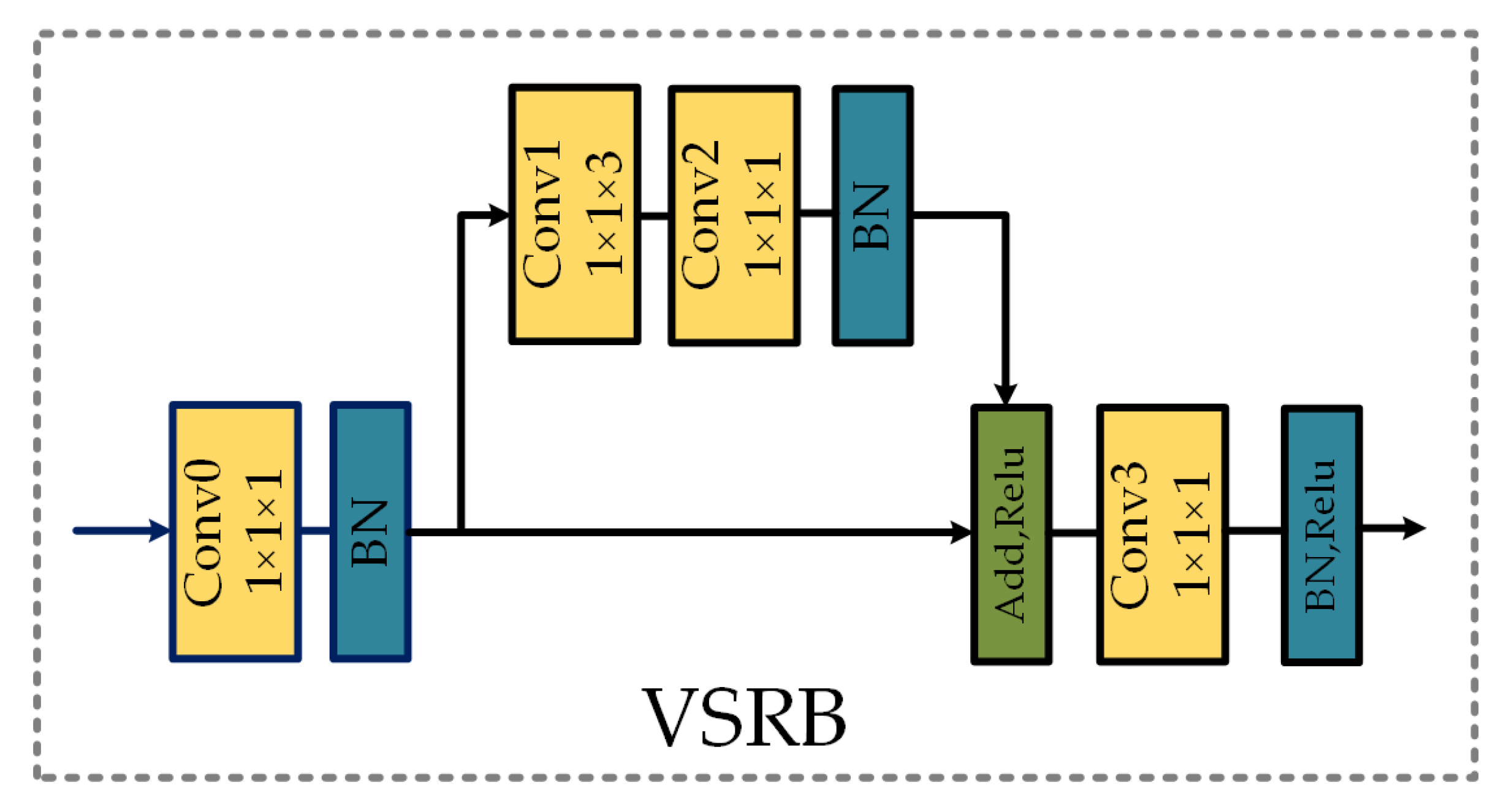
2.2. Variable Spectral Residual Block
Residual blocks have been successfully used in various deep learning applications [44]. A residual connection can be expressed as:
where and are the and feature maps, respectively, and the function F is a nonlinear transformation. Through a residual connection, the learning goal of the convolution kernel is converted to , and the residual mapping is easier to optimize than the original function F [45]. In addition, a residual block was also introduced in [45] to reduce computation and training time.
To better refine spectral–spatial features and achieve better performance, we designed the VSRB to match the dimension of the feature maps. In the proposed framework, different stages in the same subnetwork require VSRB refinement, and the VSRB architecture is shown in Figure 4. We employ a convolution layer and a batch normalization layer as the first component of the VSRB, and the layers are used to unify the number of channels, downsample spectral bands, and combine information. Then, a residual block is applied to improve feature extraction. Finally, we set a band-correction layer to adjust the band dimension and maintain dimensional consistency in the same stage of different subnetworks. It should be noted that, as the spatial dimension information is limited, we only reduce the number of spectral bands in VSRB.
2.3. Triplet Attention Mechanism
For better HSI classification performance, we propose a novel triple-attention module(CSSA) that consists of channel-wise, spectral-wise, and spatial-wise attention. The module is introduced in detail in the following.
2.3.1. Channel-Wise Attention Module
Different feature map channels in each convolution stage can be regarded as different feature representations [46,47]. A large number of channels are applied to represent different feature maps, but this results in several meaningless feature channels. Therefore, we introduce a channel-wise attention module to increase the weights of useful feature channels and weaken meaningless channels.
The proposed channel-wise attention module is shown in Figure 1a. We assume that the dimension of the input feature maps is , where and B are the channels, width, height, and bands of feature maps in each convolution stage. The input feature maps are first sent into a global average pooling (GAP) layer to aggregate spectral–spatial information into a feature vector. Then, this vector passes through a fully connected (FC) and a relu activation layer to introduce more feature representation nodes. Subsequently, another FC layer is employed to adjust the dimension of the vector back to , and a sigmoid activation function maps the feature vector to a probability vector. Finally, this probability vector is treated as a channel weight multiplied by the original feature maps. The channel weighting function can be expressed as:
where x is the input feature and is the global average pooling function. and are the first and second FC layers, respectively. is the relu function, and is the sigmoid activation layer.
2.3.2. Spectral-Wise Attention Module
Spectral bands can be represented as a continuous spectral curve that contains the value of each spectrum. For spectral classification, hundreds of spectral bands are directly used as inputs to different convolution stages. This inevitably involves some noise bands, resulting in poor classification performance. Accordingly, we propose a spectral-wise attention module to enable the network to recalibrate the importance of different spectral bands and strengthen useful spectral features.
The proposed spectral-wise attention module is shown in Figure 1b. The input feature is sent into the convolution and relu layer with only one filter to fuse information in different channels. Then, the dimension of the feature is . We set the size of the convolution kernel to , and the strategy of kernel padding to be invalid. This operation merges the spatial information and produces a feature vector with the same number of channels as that of the spectral bands. Subsequently, this vector is sent to a sigmoid function layer to obtain the probability vector. For convenience, the probability vector is upsampled to the size of the input feature. The spectral weighted feature maps by multiplying the input feature and the probability map. The spectral-wise attention module can be computed as:
where x is the input feature, is the convolution function, denotes upsampling, is the relu function, and is the sigmoid activation layer.
2.3.3. Spatial-Wise Attention Module
Environmental factors such as light, temperature, and humidity have a great influence on hyperspectral imaging. Pixels with similar spectra may belong to different classes, and pixels with different spectra may have the same label. Intra-class inconsistency and inter-class homogeneity greatly affect classification performance, and using spatial information to constrain neighboring region pixels is the key to addressing this [47]. Herein, a spatial-wise attention module is introduced to strengthen the associativity between adjacent pixels.
The proposed spatial-wise attention module is shown in Figure 1c. In contrast to the channel-wise and spectral-wise attention modules, the spatial-wise attention module is designed by using a double-branch strategy. In the two branches, we use different feature maps of different sizes as the input. Branch 1 uses the original feature maps to generate weights for each pixel of the input image. The spatial dimension of the feature maps is downsampled twice, and then the downsampled feature maps are sent to Branch 2 to obtain the probability maps. In both branches, we first use convolution with only one filter to aggregate the channel information, as in the design of the spectral-wise attention module. The feature dimensions of the two branches are and . Then, the sigmoid activation function is applied to generate probability maps. The probability result of Branch 1 directly weights the original feature maps. The probability maps of Branch 2 first upsample to , and then multiply the weighted feature maps of Branch 1. Thus, the pixels in the -region share the same weights, thereby increasing the probability that adjacent pixels belong to the same class. The spatial-wise attention module can be expressed as:
where x is the input feature, and represents the feature maps after downsampling. is the convolution function, denotes upsampling, is the relu function, and is the sigmoid activation layer.
2.3.4. Aggregation of Attention Modules
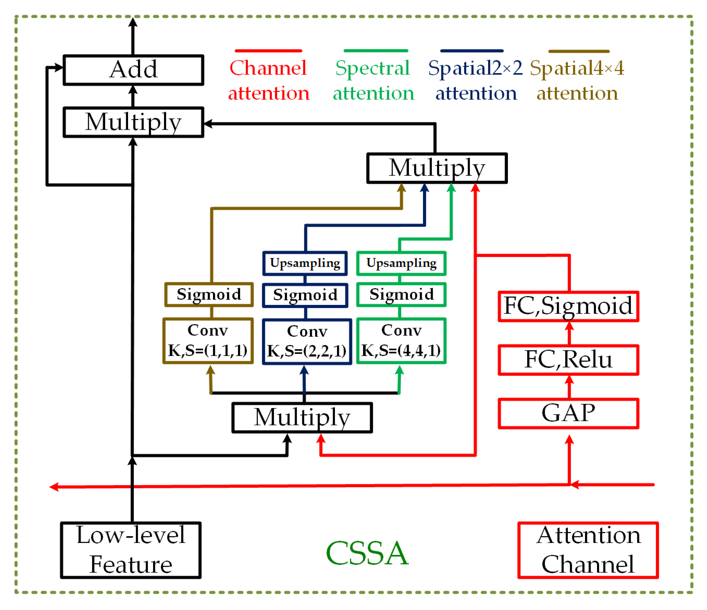
To take full advantage of the information in each dimension, we design the triple-attention block to aggregate channel, spectral, and spatial information.
As shown in Figure 5, when the attention channel is fed into the CSSA module, it first passes through the channel-wise attention module. Then, the generated channel-wise attention probability vector is multiplied by the low-level feature, and the result is sent to the spectral-wise and the double-branch spatial-wise attention module. Thereafter, the channel-wise, spectral-wise, and spatial-wise attention maps are sampled to the same size and averaged. Finally, the low-level feature is multiplied by the average weight, and the result is added to the low-level feature as the output of the CSSA module. The strategy of aggregating three weights into one is equivalent to generating a weight of the same size as that of the low-level feature, and then weighting each value of the 3D feature maps. Compared with the result of previous single or double attention mechanisms, the triple-attention mechanism comprehensively considers each dimension in the feature extraction process and adjusts the weight of the corresponding dimension.
3. Experiment Setup and Results
3.1. Data Partition
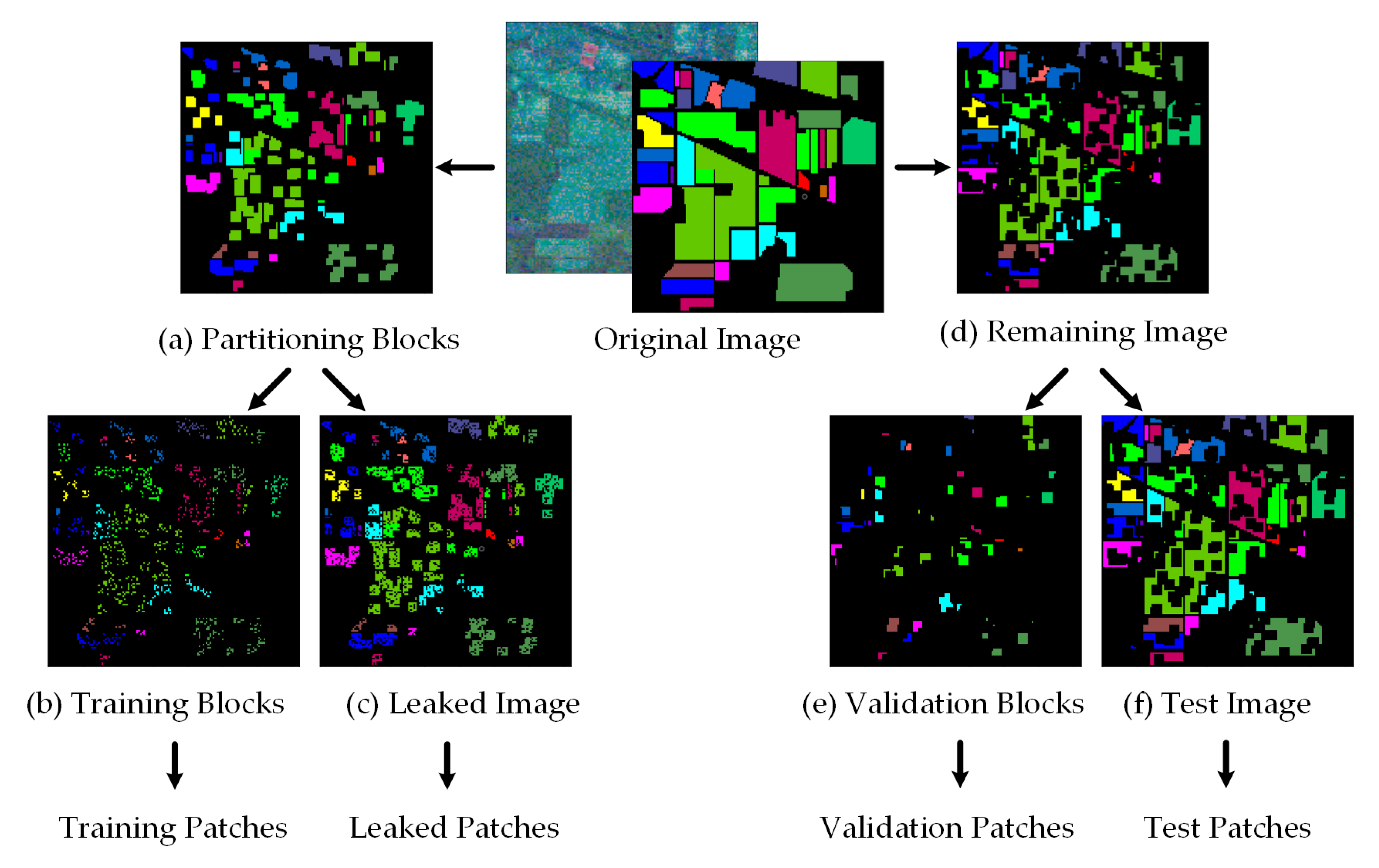
Traditional patch-based partitioning methods have been verified to have potential test information leakage in [33]. The training/test set division greatly affects the fairness of model comparison, the evaluation of framework performance, and the feasibility of practical application. Accordingly, there is an urgent need for a data-partitioning approach that allows the fair comparison of various models. To this end, some researchers have explored data-partitioning methods that do not lead to data leakage [32]. However, in [32], two potential issues should be addressed. First, some classes are missing in the training or test set of several experiments, such as C7 and C9 in the Indian Pines dataset. Second, the partitioning results of the training set indicate that the labeled pixels are clustered in each training patch. In practical applications, it is difficult to accurately mark all pixels in a neighborhood.
To address these issues, we propose a novel data partitioning standard for future studies in HSI classification. The proposed method first partitions the original image into nonoverlapping training and test blocks, and then randomly selects pixels as training pixels from the training blocks. Thereby, there is no information leakage because of the lack of overlap between the training and test blocks. The details are as follows. Before data partitioning, we determine the ratio of training pixels in the original image, and the number of labeled training pixels in each pre-partitioned training block. Therefore, the number of training blocks in each class can be expressed as:
where are the numbers of training blocks in each class ( is set to be at least 1 in each class), and refer to the number of pixels of each class in the original image. The data partitioning process is shown in Figure 6. We first divide the original image into random partitioning blocks and the remaining image, as shown in Figure 6a,d. Subsequently, we randomly reserve labeled pixels in the random partitioning blocks and save the reserved blocks as training blocks, as shown in Figure 6b. The remaining labeled pixels in the random partitioning blocks are set as leaked images, as shown in Figure 6c. Then, as shown in Figure 6e,f, we divide the remaining image into validation blocks and the remaining test image randomly. Finally, we partition the leaked image and the test image into leaked patches and test patches, respectively. In addition, we apply the same sliding window strategy as in [32] to the training and validation blocks for more training and validation patches. Furthermore, traditional data augmentation methods (i.e., flip up/down, flip right/left and rotate right/left with an angel of or ) were applied on the training and validation patches. In order to ensure the randomness in the expanded dataset, each patch will be augmented with only two of the three methods.
In the proposed partitioning method, there is no overlap between the training, validation, and test sets, and a comparison between the leaked and the test set can verify the seriousness of the potential information leakage. Moreover, this method is suitable for practical applications because it is easy to identify several pixel labels that are randomly distributed in a training block area. Furthermore, labeled pixels in a patch can also enable FCN models to extract spectral–spatial information for improved performance.
3.2. Evaluation Matrices
To evaluate the performance of the proposed TAP-Net, three popular evaluation matrices, overall accuracy (OA), average accuracy (AA), and Kappa coefficient were employed in this study. The OA metric is used to calculate the ratio of correct predictions over the total test pixels [48]. The AA metric is designed to evaluate the average performance across different classes [48]. The Kappa coefficient is calculated from a confusion matrix, and it represents a statistical measurement of agreement between the predictions and the ground-truth [48]. For all these three evaluation matrices, the higher values represent the better classification performance. Taking as the confusion matrix, represents the number of i-th class pixels that are predicted to be j-th class [49]. These three matrices are defined as follows:
3.3. Experimental Dataset
In the experiments, three well-known hyperspectral datasets were used for testing: the Salinas Valley, Pavia University, and Indian Pines datasets. Five-fold cross validation was carried out in the experiments. Moreover, each fold was repeated three times to reduce the effect of randomness. To obtain a fair comparison, we also maintained almost the same amount of data usage as in [32]. The details regarding the three dataset and the settings are as follows:
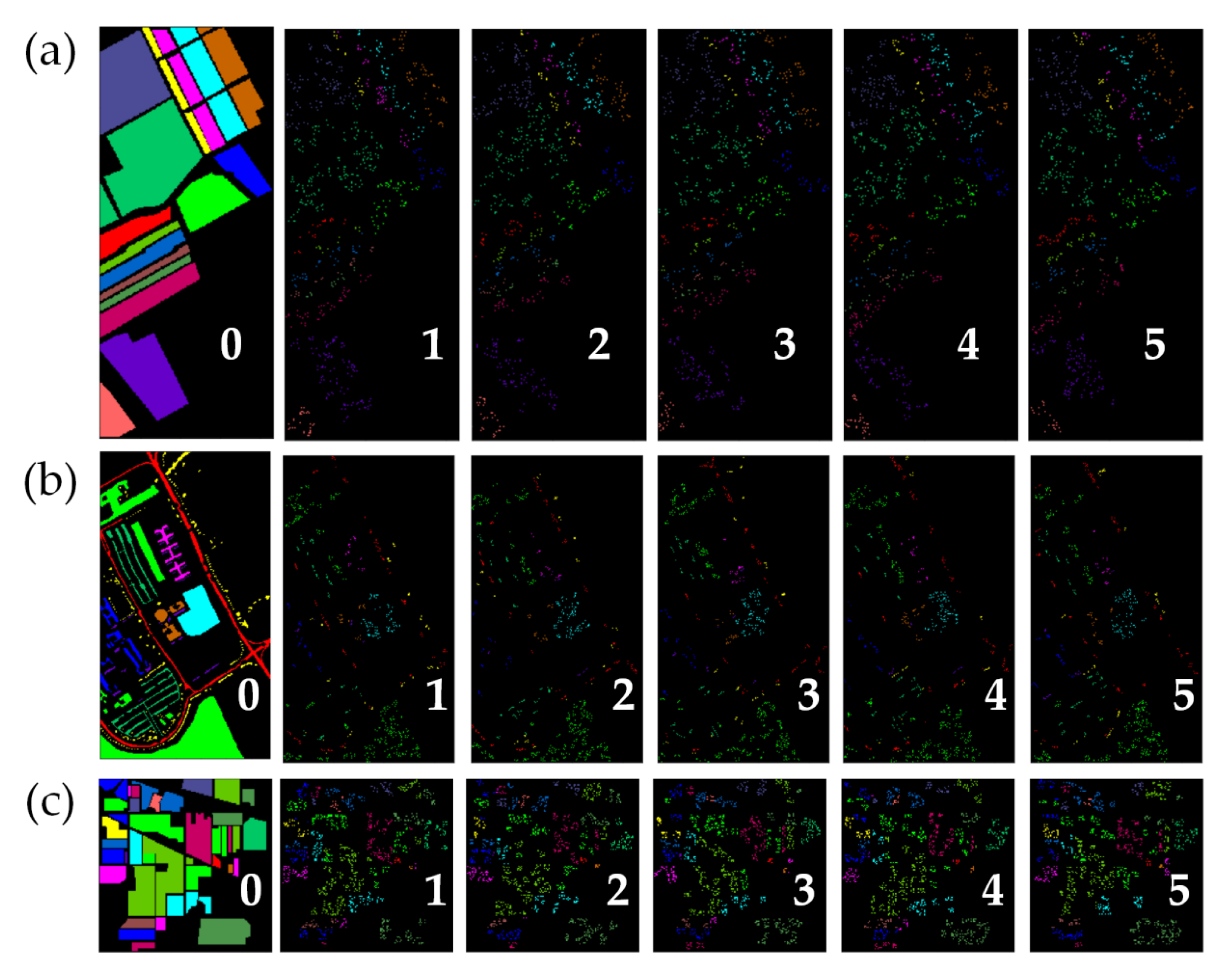
Salinas Valley: This dataset was obtained by the AVIRIS sensor (with a resolution of 3.7 m/pixel) in Salinas Valley, CA, USA. The spatial size of the dataset is pixels, the number of spectral bands is 224, and the class of ground pixels is 16. The five cross-validation folds were randomly partitioned, and the training pixels can be seen in Figure 7a(1–5), whereas the ground truth is shown in Figure 7a(0).
Pavia University: This dataset was captured by the ROSIS sensor in Pavia, northern Italy. The sensor initially photographed 115 bands, and 12 noisy bands were removed. It has pixels with a high resolution of 1.3 m/pixel and 9 land-cover classes. Figure 7b(0–5) shows a visualization of the dataset. Specifically, Figure 7b(0) shows the ground truth, and Figure 7b(1–5) shows the five random folds.
Indian Pines: This dataset was obtained by the AVIRIS sensor in Indian Pines, Northwestern Indiana. The sensor can capture 220 spectral band images with a resolution of 3.7 m/pixel. In this dataset, 20 water absorption bands were removed, and 200 spectral bands remained with a spatial size of pixels. The ground truth and the distribution of the five folds are shown in Figure 7c(0–5).
To obtain a fair comparison with other methods, we used the same number of training pixels as in [32]. As shown in Table 1, Table 2 and Table 3, we divided the labeled pixels into training, validation, leaked, and test sets. Owing to the randomness of the data partitioning method, the values in Table 1, Table 2 and Table 3 were obtained by taking the average of different folds. In the Salinas Valley dataset, 2017.2, 2062.2, 16,071.4, and 33,978.2 labeled pixels were divided into training, validation, leaked, and test sets, respectively. The division results are 2721.4/2758.6/11,822/25,474 and 1187.8/1144.4/3318.4/4598.4 for Pavia University and Indian Pines, respectively. In the experiment, the proportion of leaked pixels reached 47.30%, 46.41%, and 72.16% compared with test pixels. In fact, the number of leaked pixels in the traditional centered partitioning method is significantly greater, and therefore the resulting information leakage may yield more overoptimistic results.
3.4. Parameter Setting and Network Configuration
In data partitioning, considering the different spatial sizes and the limited pixels in each dataset, we set different block and patch sizes when dividing different datasets. In Salinas Valley, we selected the block size as , and the patch size as to ensure the extraction of spatial information. This selection can also provide sufficiently many training patches by using the traditional sliding window strategy. The number of labeled pixels in each training block () was set to 10 in the experiment. Similarly, the block-patch size was 12–10 and 6–4, and the parameter was set to 15 and 8 for Pavia University and Indian Pines, respectively. in the three datasets is a free variable that is used to control the proportions of the training, validation, and test sets.
In the framework design, we used nearly the same parameter settings for the three datasets. As shown in Table 4, with the Salinas Valley as an example, the triple-attention parallel network consists of four subnetworks, and each subnetwork is divided into four stages. In each subnetwork, two neighbor stages are connected by VSRB for efficient feature extraction. The kernel size of the VSRB and the output size of the feature maps in each stage are shown in Table 4. In adjacent subnetworks, the feature maps in the preceding subnetwork are filtered by the triple-attention module and are fused with the maps in the corresponding stage in the succeeding subnetwork. For example, stage 1, 2 and 3 of subnetwork 0 is fused with stage 1, 2 and 3 of subnetwork 2, respectively. In the kernel size settings, the first stage of each subnetwork is an aggregation layer. A convolution kernel with a size of is used to aggregate the channel–spectral–spatial information. In the remaining stages, a convolution kernel is used to enhance the extraction of spectral information.
The TAP-Net was implemented in Python 3.6 and Keras 2.2.4. The Adam (beta_1 = 0.9, beta_2 = 0.999, epsilon = ) was employed as the optimizer. The learning rate was initially set as 0.01, and shrunk to 1/10 of the previous value after every 20 epochs. The batch size was set to 32. We utilized focal loss as the loss function, which is designed to reduce the impact of easy samples [50]. All the experiments were performed with the same configuration on the platform with Intel i7-8700K, 32 GB RAM, and NVIDIA GeForce GTX 1080 GPU.
4. Classification Result
We compare the TAP network with other state-of-the-art CNN-based methods that do not exhibit information leakage. Furthermore, to evaluate the contribution of each module to the final performance, we conducted experiments with or without a parallel network and the triple-attention module. In the comparison, we used the following networks:
VHIS was proposed in [33], where the information leakage problem in traditional CNN-based methods was explained. The authors introduced a 1D CNN-based network to extract spectral features and classify pixels without information leakage.
DA-VHIS was introduced in [34], where three data augmentation methods were proposed to generate more training samples. We report the best performance of these three data augmentation methods in the comparison.
Auto-CNN was proposed in [51], where a 1D Auto-CNN was applied to optimize the classifier without test information leakage. The best framework is automatically selected for HSI classification.
SS3FCN was introduced in [32], where a data partitioning strategy was designed to avoid information leakage. This strategy also allows the exploration of spectral–spatial information by the proposed 1D and 3D double-branch networks.
SerialNet was shown in Figure 8a. It is a serial network with the same number of stages as in the proposed TAP-Net. Moreover, the VSRB module are used for feature extraction, and the corresponding parameter setting and network configuration are the same as TAP-Net.
ParallelNet was shown in Figure 8b. The ParallelNet, consists of VSRB module and parallel module, is compared with serial net to validate the performance of parallel module. The hyper parameter and network configuration are same as that in TAP-Net. The main difference between the ParallelNet and TAP-Net is that there is no attention module in ParallelNet.
4.1. Results on Salinas Valley
The average classification results and standard deviation on the Salinas Valley dataset are listed in Table 5. It can be seen that the proposed method achieves the best performance when as many training samples are used as in SS3FCN, and fewer samples than in VHIS, GAN-VHIS, and AutoCNN. Compared with traditional spectral classification methods (VHIS, GAN-VHIS, and AutoCNN), TAP-Net, by using spectral–spatial information, improves accuracy by more than 10%. The OA&AA by TAP-Net increased from 81.32% & 86.13% to 90.31% & 93.18%, compared with that by other 3DCNN-based methods (SS3FCN). Regarding the proposed module, ParallelNet improves OA & AA & Kappa by 2.28% & 2.10% & 2.8% compared with SerialNet through multi-scale spectral information fusion and the anti-cross-layer connection. The triple-attention-based TAP-Net also improves OA & AA & Kappa by 1.37% & 0.45% & 3.5% compared with ParallelNet. Considering the accuracy of the frameworks under comparison, the proposed framework is more robust even with a small number of training samples. Figure 9 shows classification maps by certain methods only, as the other methods are not described in sufficient detail to reproduce the classification maps.
4.2. Results on Pavia University
The OA, AA, and class-specific accuracy obtained by different methods on the Pavia University dataset are shown in Table 6. As in the case of Salinas Valley, SerialNet, ParallelNet, and the proposed TAP-Net achieve significantly better OA & AA than VHIS, GAN-VHIS, AutoCNN, and SS3FCN. In addition, the data partitioning method, parallel framework, and triple-attention module are highly successful. In the comparison of each sub-module, the accuracy of C6 increased from 23.59% to 56.58% by introducing the proposed data partitioning method. The OA & AA & Kappa of the parallel framework increased by 2.84% & 5.47% & 1.5% compared with that of the serial module. The OA & AA & Kappa of the proposed TAP-Net increased from 86.30% & 82.01% & 86.6% to 91.64% & 87.45% & 89.2% after the addition of the triple-attention module to ParallelNet. Finally, compared with the state-of-the-art spectral–spatial framework (SS3FCN), TAP-Net achieved 11.75% & 10.85% better performance than SS3FCN in terms of OA and AA. Figure 10 the classification maps obtained by some of the methods under comparison.
4.3. Results on Indian Pines
The overall classification results and accuracy of each class are shown in Table 7. Regarding the Indian Pines dataset, the number of pixels in each class is quite imbalanced, and this significantly affects the results of the experiment. For example, VHIS, GAN-VHIS, AutoCNN, and SS3FCN only obtain an accuracy of 0 & 23.8% & 35.63% 20.14% & 21% for the C7 class. The same occurs in the classification of C1 and C9. These classes of samples are not sufficiently large to learn differentiable features in other frameworks. In the proposed method, TAP-Net achieves an accuracy of 70.98%, 80.40%, and 70.03% in the classification of C1, C7, and C9, respectively. This demonstrates that TAP-Net can better extract features in these limited classes and achieve higher classification accuracy with almost the same number of training pixels. In addition, the proposed framework achieves the best performance, with the OA & AA & Kappa of TAP-Net is 81.35% & 78.85% & 0.787, which is significantly better than the performance of the other frameworks. The classification maps of some frameworks are shown in Figure 11.
5. Analysis and Discussion
The results in Section 4 demonstrate that the proposed method yields the best results in HSI classification, particularly for classes that are difficult to classify using other methods. Herein, we explore the effect of various factors on model performance. The leakage of test information, block-patch size, number of labeled pixels in each block, and the effect between different attention mechanisms are discussed for future reference.
5.1. Effect of Information Leakage
We now revisit the information leakage problem, which may reduce the credibility of the results obtained by existing traditional data partitioning strategies and classification networks. As shown in Figure 12, we compare the average results of leaked and non-leaked datasets generated by the same training model. “Real acc” is obtained from non-leaked test samples that do not overlap with the training block, whereas “Leaked acc” is obtained from samples with information leakage. In Figure 12a, the accuracy of all 16 classes and OA & AA in Real acc is lower than in Leaked acc. Among them, the largest gap between Real acc and Leaked acc is in C15, and the performance gap between the two test sets is more than 10% in the classification of C15. Moreover, there is an optimistic performance of approximately 3% in OA & AA for Leaked acc. In Figure 12b, C3, C6, and C7 are the main factors that cause accuracy distortion; the largest performance gap between the two test sets increases by up to 25%. The OA & AA values also increase from 91.64% & 87.45% to 97.91% & 95.65%. The most serious accuracy distortion occurs in the Indian pines dataset, as shown in Figure 12c, where almost all classes exhibit highly optimistic performance. The real OA & AA in this dataset increases by 12.08% & 12.47% on the leaked test set. In general, we hope that an accuracy comparison between the real and leaked test sets will enable recognizing and avoiding the information leakage problem in future studies.
5.2. Effect of Block-Patch Size
To achieve the best classification results, we now discuss the effect of different block-patch sizes. In this study, blocks are set to select the training and validation data. The size of these blocks in the experiment determines the spatial information of the training and validation samples. Moreover, the number of training and validation samples is controlled by the patch size in the sliding window strategy. We empirically set the difference between block and patch size to 2 in the comparison experiment. The results on the three datasets are shown in Table 8. For example, in the Salinas Valley dataset, the proposed TAP-Net achieves the highest accuracy with an OA/AA of 90.31%/93.18% when the block-patch size is 10–8. Performance decreases gradually with an increase or decrease in the block-patch size. In fact, the spatial information in the training patch decreases if smaller block size is used. Conversely, the correlation between pixels decreases when the same number of labeled pixels are randomly distributed in larger blocks. Similar results are obtained on the other datasets; on the Pavia University (10–8) and the Indian Pines (6–4) datasets, the best performance is achieved, with an OA & AA of 91.64% & 87.45% and 81.35% & 78.85%, respectively. It should be noted that when the block-patch size is set to 10–8 for Indian Pines, all the labeled pixels appear in the training set, and thus no test results are obtained.
5.3. Effect of the Number of Labeled Pixels in Each Block
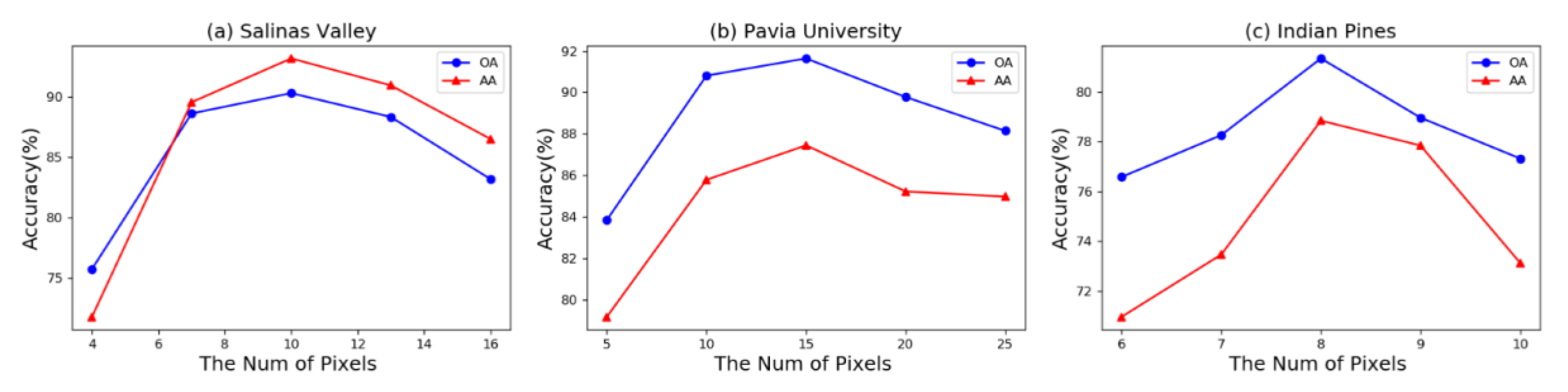
The labeled pixels in each block (Np in the data partitioning part) determine the distribution of the training pixels. In this study, the number of training, validation, and test pixels have a fixed upper limit. For example, in the training set, the total number of training blocks decreases if more labeled pixels appear in each training block. As the sampling blocks in a class decrease, the location of partitioning blocks within the class becomes unbalanced. As the percentage of labeled pixels in a training block decreases, more blocks should be partitioned to ensure that the same number of pixels are used for training. However, the continuity of spatial information within the block will be reduced because of the decreased labeled pixels. The balance between the number of blocks and pixels is important in classification. Figure 13 shows the effect of different Np in different datasets. The Salinas Valley, Pavia University, and Indian pine datasets achieve the best performance when Np is set to 10, 15, and 8, respectively.
5.4. Advantages and Limitations
The problem of information leakage leads to overoptimistic performance, which might be unreliable. In this paper, a novel data partitioning strategy without information leakage and a well designed deep learning architecture are proposed. Although the proposed modules are meaningful for HSI classification, there are still a few limitations needed to be addressed in future research.
5.4.1. Impact of the Attention Module
To verify the effectiveness of the triple-attention module, we added a channel–spectral attention module (ParallelNet-CS), spectral–spatial attention module (ParallelNet-SS), and triple-attention module (TAP-Net) to ParallelNet for comparison. For simplicity, we take the Pavia University as an example, and the results of these attention-based ParallelNet are shown in Table 9. Evidently, the proposed triple-attention module provides the best performance, with OA & AA of the module is 91.64% & 87.45%, which is significantly better than that of other attention modules. Moreover, the smaller standard derivation of OA, AA and Kappa score corresponding to TAP-Net indicates its better stability under the same parameter settings. Similar results shown in supplementary material were observed on the Salinas Valley and Indian Pines dataset.
The statistical testing can make claims about whether the distribution of one set of results are different from another set. In this study, we execute a two-tailed Wilcoxon’s test over per-class AA to verify if the differences between the investigated modules are statistically important. The statistical difference between SerialNet, ParallelNet, ParallelNet-SS, ParallelNet-CS and TAP-Net is shown in Table 10, demonstrating that the proposed triple attention module has significant improvement (p-value < 0.05) over SerialNet, ParallelNet, ParallelNet-CS and ParallelNet-SS. Similarly, the channel–spectral and spectral–spatial attention module also delivered large improvement in comparing with SerialNet and ParallelNet without attention. However, there is no statistical difference between ParallelNet-SS and ParallelNet-CS, although the performance of ParallelNet-CS is slightly better than that of ParallelNet-SS.
5.4.2. Impact of Data Splits and Augmentation
Data partitioning has a great influence on the classification performance, as the distribution of partitioned training and test sets might be balanced or unbalanced (i.e., some classes are missed in the training or test set). In contrast to VHIS [33], our proposed method is able to provide a more balanced data splits. As shown in Table 11, the proposed TAP-Net achieves better performance with both data split strategies. It demonstrates that the importance of data split strategy and the effectiveness of the proposed TAP-Net.
In [34], the authors introduced three training- and test-time data augmentation techniques. The VHIS with data augmentation consistently got better performance than that without data augmentation across three benchmark datasets, with an improvement of 0.58–14.54% on OA/AA. However, these pixel-wise augmentation methods are not applicable for 3D network. Inspired by [34], we applied a simple data augmentation strategy, including flip and rotate. As shown in Table 11, the performance of TAP-Net with data augmentation are significantly better than that without data augmentation. Taking the Salina Valley dataset for instance, the overall accuracy, average accuracy, and the Kappa is 90.31%, 93.18% and 0.881 respectively with data augmentation, whereas the corresponding value is 85.57%, 89.04% and 0.850 without data augmentation. However, developing more sophiscated data augmentation ways and evaluating the difference between them is outside the scope of this paper, and we will work on this topic in our future research.
6. Conclusions
Hyperspectral image classification, which aims to assign a unique label to each pixel of HSI, is a critical step for HSI analysis. Although CNN-based models have exhibited promising performance, most CNN-based HSI classification methods have potential training-test information leakage, leading to overoptimistic results. In this study, we proposed a triple-attention-based parallel network and a novel data partitioning strategy for pixel-wise classification. First, we introduced a parallel network that utilizes parallel subnetworks with the same spatial resolution and repeatedly reuses high-level feature maps of preceding subnetworks to refine the segmentation map. Subsequently, to further improve the performance of the classifier, we proposed the triple-attention module to strengthen useful information and weaken meaningless information. Furthermore, we introduced a novel data partitioning method to serve as a standard for future research in this field. It provides a balanced training/test-set without information leakage, and is suitable for practical HSI annotations. Ablation studies regarding to the attention mechanism, parallel network and data split strategy demonstrate the effectiveness of these modules across three benchmark datasets. The CSSA and Parallel Net module used in TAP-Net can be used as separate modules in other algorithms. Considering the effectiveness of data augmentation, a more sophisticated ways to enhance the HSI data is highly desired, and we will focus it in future study.
Supplementary Materials
The following are available online at https://0-www-mdpi-com.brum.beds.ac.uk/2072-4292/13/2/324/s1.
Author Contributions
Conceptualization, X.Z. and L.Q.; methodology, L.Z. and X.Z.; software, X.Z.; validation, L.Q.; investigation, X.Z.; resources, L.Z. and L.Q.; data curation, J.Z.; writing-original draft preparation, X.Z. and L.Z.; writing-review and editing, J.Z. and L.Q.; visualization, X.Z.; supervision, L.Q.; project administration, L.Q.; funding acquisition, L.Z. and L.Q. All authors have read and agreed to the published version of the manuscript.
Funding
This work was supported in part by the National Natural Science Foundation of China under Grants 61901003 and 61871411, in part by the Natural Science Foundation of Jiangsu Province under Grant BK20190623, and in part by the University Synergy Innovation Program of Anhui Province under Grant GXXT-2019-008.
Institutional Review Board Statement
Not applicable.
Informed Consent Statement
Not applicable.
Data Availability Statement
The hyperspectral images utilized in this study are freely available at http://www.ehu.eus/ccwintco/index.php/Hyperspectral_Remote_Sensing_Scenes.
Acknowledgments
We thank all the people involved in the study.
Conflicts of Interest
The authors declare no conflict of interest.
References
- Ma, X.; Fu, A.; Wang, J.; Wang, H.; Yin, B. Hyperspectral image classification based on deep deconvolution network with skip architecture. IEEE Trans. Geosci. Remote Sens. 2018, 56, 4781–4791. [Google Scholar] [CrossRef]
- Li, Y.; Zhang, H.; Shen, Q. Spectral–spatial classification of hyperspectral imagery with 3D convolutional neural network. Remote Sens. 2017, 9, 67. [Google Scholar] [CrossRef] [Green Version]
- Zurqani, H.A.; Post, C.J.; Mikhailova, E.A.; Cope, M.P.; Allen, J.S.; Lytle, B.A. Evaluating the integrity of forested riparian buffers over a large area using LiDAR data and Google Earth Engine. Sci. Rep. 2020, 10, 1–16. [Google Scholar] [CrossRef] [PubMed]
- Zhong, Z.; Li, J.; Luo, Z.; Chapman, M. Spectral–spatial residual network for hyperspectral image classification: A 3-D deep learning framework. IEEE Trans. Geosci. Remote Sens. 2017, 56, 847–858. [Google Scholar] [CrossRef]
- Van Ruitenbeek, F.; van der Werff, H.; Bakker, W.; van der Meer, F.; Hein, K. Measuring rock microstructure in hyperspectral mineral maps. Remote Sens. Environ. 2019, 220, 94–109. [Google Scholar] [CrossRef]
- Wei, L.; Xiao, X.; Wang, Y.; Zhuang, X.; Wang, J. Research on the shortwave infrared hyperspectral imaging technology based on Integrated Stepwise filter. Infrared Phys. Technol. 2017, 86, 90–97. [Google Scholar] [CrossRef]
- Li, S.; Song, W.; Fang, L.; Chen, Y.; Ghamisi, P.; Benediktsson, J.A. Deep learning for hyperspectral image classification: An overview. IEEE Trans. Geosci. Remote Sens. 2019, 57, 6690–6709. [Google Scholar] [CrossRef] [Green Version]
- Fang, B.; Li, Y.; Zhang, H.; Chan, J.C.W. Hyperspectral images classification based on dense convolutional networks with spectral-wise attention mechanism. Remote Sens. 2019, 11, 159. [Google Scholar] [CrossRef] [Green Version]
- Tarabalka, Y.; Fauvel, M.; Chanussot, J.; Benediktsson, J.A. SVM-and MRF-based method for accurate classification of hyperspectral images. IEEE Geosci. Remote Sens. Lett. 2010, 7, 736–740. [Google Scholar] [CrossRef] [Green Version]
- Xing, Z.; Zhou, M.; Castrodad, A.; Sapiro, G.; Carin, L. Dictionary learning for noisy and incomplete hyperspectral images. SIAM J. Imaging Sci. 2012, 5, 33–56. [Google Scholar] [CrossRef]
- Fauvel, M.; Chanussot, J.; Benediktsson, J.A. A spatial–spectral kernel-based approach for the classification of remote-sensing images. Pattern Recognit. 2012, 45, 381–392. [Google Scholar] [CrossRef]
- Chen, Y.; Zhao, X.; Jia, X. Spectral–spatial classification of hyperspectral data based on deep belief network. IEEE J. Sel. Top. Appl. Earth Obs. Remote Sens. 2015, 8, 2381–2392. [Google Scholar] [CrossRef]
- Fauvel, M.; Tarabalka, Y.; Benediktsson, J.A.; Chanussot, J.; Tilton, J.C. Advances in spectral–spatial classification of hyperspectral images. Proc. IEEE 2012, 101, 652–675. [Google Scholar] [CrossRef] [Green Version]
- Zhong, P.; Gong, Z. A hybrid DBN and CRF model for spectral–spatial classification of hyperspectral images. Stat. Optim. Inf. Comput. 2017, 5, 75. [Google Scholar] [CrossRef] [Green Version]
- Sun, L.; Wu, Z.; Liu, J.; Xiao, L.; Wei, Z. Supervised spectral–spatial hyperspectral image classification with weighted Markov random fields. IEEE Trans. Geosci. Remote Sens. 2014, 53, 1490–1503. [Google Scholar] [CrossRef]
- Ghamisi, P.; Maggiori, E.; Li, S.; Souza, R.; Tarablaka, Y.; Moser, G.; De Giorgi, A.; Fang, L.; Chen, Y.; Chi, M.; et al. New frontiers in spectral–spatial hyperspectral image classification: The latest advances based on mathematical morphology, Markov random fields, segmentation, sparse representation, and deep learning. IEEE Geosci. Remote Sens. Mag. 2018, 6, 10–43. [Google Scholar] [CrossRef]
- Fang, X.; Zou, L.; Li, J.; Sun, L.; Ling, Z.H. Channel adversarial training for cross-channel text-independent speaker recognition. In Proceedings of the ICASSP 2019—2019 IEEE International Conference on Acoustics, Speech and Signal Processing (ICASSP), Brighton, UK, 12–17 May 2019; pp. 6221–6225. [Google Scholar]
- Liu, H.; Du, F.; Tang, X.; Liu, H.; Yu, Z. Network Architecture Reasoning Via Deep Deterministic Policy Gradient. In Proceedings of the 2020 IEEE International Conference on Multimedia and Expo (ICME), London, UK, 6–10 July 2020; pp. 1–6. [Google Scholar]
- Chen, X.; Li, Y.; Hu, R.; Zhang, X.; Chen, X. Hand Gesture Recognition based on Surface Electromyography using Convolutional Neural Network with Transfer Learning Method. IEEE J. Biomed. Health Inform. 2020. [Google Scholar] [CrossRef]
- Wang, D.; Mao, K.; Ng, G.W. Convolutional neural networks and multimodal fusion for text aided image classification. In Proceedings of the 2017 20th International Conference on Information Fusion (Fusion), Xi’an, China, 10–13 July 2017; pp. 1–7. [Google Scholar]
- Ma, W.; Yang, Q.; Wu, Y.; Zhao, W.; Zhang, X. Double-branch multi-attention mechanism network for hyperspectral image classification. Remote Sens. 2019, 11, 1307. [Google Scholar] [CrossRef] [Green Version]
- Yang, J.; Zhao, Y.Q.; Chan, J.C.W.; Xiao, L. A Multi-Scale Wavelet 3D-CNN for Hyperspectral Image Super-Resolution. Remote Sens. 2019, 11, 1557. [Google Scholar] [CrossRef] [Green Version]
- Zou, L.; Zheng, J.; Miao, C.; Mckeown, M.J.; Wang, Z.J. 3D CNN based automatic diagnosis of attention deficit hyperactivity disorder using functional and structural MRI. IEEE Access 2017, 5, 23626–23636. [Google Scholar] [CrossRef]
- Wang, C.; Ma, N.; Ming, Y.; Wang, Q.; Xia, J. Classification of hyperspectral imagery with a 3D convolutional neural network and JM distance. Adv. Space Res. 2019, 64, 886–899. [Google Scholar] [CrossRef]
- Pan, B.; Xu, X.; Shi, Z.; Zhang, N.; Luo, H.; Lan, X. DSSNet: A Simple Dilated Semantic Segmentation Network for Hyperspectral Imagery Classification. IEEE Geosci. Remote Sens. Lett. 2020. [Google Scholar] [CrossRef]
- Pan, B.; Shi, Z.; Xu, X. MugNet: Deep learning for hyperspectral image classification using limited samples. ISPRS J. Photogramm. Remote Sens. 2018, 145, 108–119. [Google Scholar] [CrossRef]
- Fang, X.; Gao, T.; Zou, L.; Ling, Z. Bidirectional Attention for Text-Dependent Speaker Verification. Sensors 2020, 20, 6784. [Google Scholar] [CrossRef] [PubMed]
- Wu, F.; Chen, F.; Jing, X.Y.; Hu, C.H.; Ge, Q.; Ji, Y. Dynamic attention network for semantic segmentation. Neurocomputing 2020, 384, 182–191. [Google Scholar] [CrossRef]
- Tao, W.; Li, C.; Song, R.; Cheng, J.; Liu, Y.; Wan, F.; Chen, X. EEG-based emotion recognition via channel-wise attention and self attention. IEEE Trans. Affect. Comput. 2020. [Google Scholar] [CrossRef]
- Ribalta Lorenzo, P.; Tulczyjew, L.; Marcinkiewicz, M.; Nalepa, J. Hyperspectral Band Selection Using Attention-Based Convolutional Neural Networks. IEEE Access 2020, 8, 42384–42403. [Google Scholar] [CrossRef]
- Pan, E.; Ma, Y.; Mei, X.; Dai, X.; Fan, F.; Tian, X.; Ma, J. Spectral-Spatial Classification of Hyperspectral Image based on a Joint Attention Network. In Proceedings of the IGARSS 2019—2019 IEEE International Geoscience and Remote Sensing Symposium, Yokohama, Japan, 28 July–2 August 2019; pp. 413–416. [Google Scholar]
- Zou, L.; Zhu, X.; Wu, C.; Liu, Y.; Qu, L. Spectral–Spatial Exploration for Hyperspectral Image Classification via the Fusion of Fully Convolutional Networks. IEEE J. Sel. Top. Appl. Earth Obs. Remote Sens. 2020, 13, 659–674. [Google Scholar] [CrossRef]
- Nalepa, J.; Myller, M.; Kawulok, M. Validating hyperspectral image segmentation. IEEE Geosci. Remote Sens. Lett. 2019, 16, 1264–1268. [Google Scholar] [CrossRef] [Green Version]
- Nalepa, J.; Myller, M.; Kawulok, M. Training-and test-time data augmentation for hyperspectral image segmentation. IEEE Geosci. Remote Sens. Lett. 2019, 17, 292–296. [Google Scholar] [CrossRef]
- Hu, W.; Huang, Y.; Wei, L.; Zhang, F.; Li, H. Deep convolutional neural networks for hyperspectral image classification. J. Sens. 2015, 2015. [Google Scholar] [CrossRef] [Green Version]
- Chen, Y.; Jiang, H.; Li, C.; Jia, X.; Ghamisi, P. Deep feature extraction and classification of hyperspectral images based on convolutional neural networks. IEEE Trans. Geosci. Remote Sens. 2016, 54, 6232–6251. [Google Scholar] [CrossRef] [Green Version]
- Sun, K.; Xiao, B.; Liu, D.; Wang, J. Deep high-resolution representation learning for human pose estimation. In Proceedings of the IEEE Conference on Computer Vision and Pattern Recognition, Long Beach, CA, USA, 16–20 June 2019; pp. 5693–5703. [Google Scholar]
- Li, H.; Xiong, P.; Fan, H.; Sun, J. Deep Feature Aggregation for Real-Time Semantic Segmentation. In Proceedings of the IEEE Conference on Computer Vision and Pattern Recognition, Long Beach, CA, USA, 16–20 June 2019. [Google Scholar]
- McNeely-White, D.; Beveridge, J.R.; Draper, B.A. Inception and ResNet features are (almost) equivalent. Cogn. Syst. Res. 2020, 59, 312–318. [Google Scholar] [CrossRef]
- Wang, T.; Wang, G.; Tan, K.E.; Tan, D. Hyperspectral Image Classification via Pyramid Graph Reasoning. In Advances in Visual Computing; Bebis, G., Yin, Z., Kim, E., Bender, J., Subr, K., Kwon, B.C., Zhao, J., Kalkofen, D., Baciu, G., Eds.; Springer International Publishing: Cham, Switzerland, 2020; pp. 707–718. [Google Scholar]
- Huang, G.; Liu, Z.; van der Maaten, L.; Weinberger, K.Q. Densely Connected Convolutional Networks. In Proceedings of the IEEE Conference on Computer Vision and Pattern Recognition (CVPR), Honolulu, HI, USA, 21–26 July 2017. [Google Scholar]
- Zeng, Z.; Xie, W.; Zhang, Y.; Lu, Y. RIC-Unet: An improved neural network based on Unet for nuclei segmentation in histology images. IEEE Access 2019, 7, 21420–21428. [Google Scholar] [CrossRef]
- Ibtehaz, N.; Rahman, M.S. MultiResUNet: Rethinking the U-Net architecture for multimodal biomedical image segmentation. Neural Netw. 2020, 121, 74–87. [Google Scholar] [CrossRef]
- Ren, F.; Liu, W.; Wu, G. Feature Reuse Residual Networks for Insect Pest Recognition. IEEE Access 2019, 7, 122758–122768. [Google Scholar] [CrossRef]
- He, K.; Zhang, X.; Ren, S.; Sun, J. Deep residual learning for image recognition. In Proceedings of the IEEE Conference on Computer Vision and Pattern Recognition, Las Vegas, NV, USA, 26 June–1 July 2016; pp. 770–778. [Google Scholar]
- Xi, J.; Yuan, X.; Wang, M.; Li, A.; Li, X.; Huang, Q. Inferring subgroup-specific driver genes from heterogeneous cancer samples via subspace learning with subgroup indication. Bioinformatics 2020, 36, 1855–1863. [Google Scholar] [CrossRef]
- Fu, J.; Liu, J.; Tian, H.; Li, Y.; Bao, Y.; Fang, Z.; Lu, H. Dual attention network for scene segmentation. In Proceedings of the IEEE Conference on Computer Vision and Pattern Recognition, Long Beach, CA, USA, 16–20 June 2019; pp. 3146–3154. [Google Scholar]
- Mei, X.; Pan, E.; Ma, Y.; Dai, X.; Huang, J.; Fan, F.; Du, Q.; Zheng, H.; Ma, J. Spectral–spatial attention networks for hyperspectral image classification. Remote Sens. 2019, 11, 963. [Google Scholar] [CrossRef] [Green Version]
- Sun, H.; Zheng, X.; Lu, X.; Wu, S. Spectral–Spatial Attention Network for Hyperspectral Image Classification. IEEE Trans. Geosci. Remote Sens. 2020, 58, 3232–3245. [Google Scholar] [CrossRef]
- Lin, T.; Goyal, P.; Girshick, R.; He, K.; Dollár, P. Focal Loss for Dense Object Detection. In Proceedings of the 2017 IEEE International Conference on Computer Vision (ICCV), Venice, Italy, 22–29 October 2017; pp. 2999–3007. [Google Scholar]
- Chen, Y.; Zhu, K.; Zhu, L.; He, X.; Ghamisi, P.; Benediktsson, J.A. Automatic Design of Convolutional Neural Network for Hyperspectral Image Classification. IEEE Trans. Geosci. Remote Sens. 2019, 57, 7048–7066. [Google Scholar] [CrossRef]
Figure 1.
Various attention modules, including (a) channel-wise attention, (b) spectral-wise attention and (c) spatial-wise attention. C, W, H and B represent the number of channels, width, height and number of bands respectively. For easier understanding, weighted channels, weighted bands, and weighted pixels are represented by different colors. GAP denotes the global average pooling and FC denotes the fully connected layer. Conv represents the convolutional layer.

Figure 2.
Channel–spectral–spatial-attention parallel network. Each row and column represents the same subnetwork and the same convolution stage, respectively; VSRB represents the variable spectral residual block; CSSA represents the channel–spatial–spectral-attention module.
Figure 2.
Channel–spectral–spatial-attention parallel network. Each row and column represents the same subnetwork and the same convolution stage, respectively; VSRB represents the variable spectral residual block; CSSA represents the channel–spatial–spectral-attention module.

Figure 3.
Various CNN frameworks: (a) Serial network with cross-layer connectivity, (b) network with cross-layer connectivity and multi-scale context fusion, (c) common two-branch fusion network in HSI classification, and (d) example of the proposed parallel network with two subnetworks (SN1, SN2).
Figure 3.
Various CNN frameworks: (a) Serial network with cross-layer connectivity, (b) network with cross-layer connectivity and multi-scale context fusion, (c) common two-branch fusion network in HSI classification, and (d) example of the proposed parallel network with two subnetworks (SN1, SN2).

Figure 4.
The variable spectral residual block used for replacing the convolution operation in each subnetwork. BN represents the batch normalization, and Conv denotes the convolutional layer.
Figure 4.
The variable spectral residual block used for replacing the convolution operation in each subnetwork. BN represents the batch normalization, and Conv denotes the convolutional layer.

Figure 5.
The triple-attention module, involving in channel-, spectral- and spatial- attention (CSSA). GAP, FC, K, S represents global average pooling, the fully connected layer, the kernel size and the stride, respectively. The triple-attention module(CSSA) has two inputs: (1) the feature maps at the highest level of the preceding subnetwork, and (2) the corresponding low-level feature maps of the same stage. The total weight is generated by aggregating the three types of attention modules.

Figure 6.
Training-test set splits: (a) random partitioning blocks, (b) training blocks, (c) leaked image, (d) remaining image, (e) validation blocks, (f) test image.
Figure 6.
Training-test set splits: (a) random partitioning blocks, (b) training blocks, (c) leaked image, (d) remaining image, (e) validation blocks, (f) test image.

Figure 7.
Training pixels in (a) Salinas Valley dataset, (b) Pavia University dataset, (c) Indian Pines dataset. Subfigure 0 in each dataset is the ground truth for the corresponding dataset. The other subfigures represent the training pixels for different folds.
Figure 7.
Training pixels in (a) Salinas Valley dataset, (b) Pavia University dataset, (c) Indian Pines dataset. Subfigure 0 in each dataset is the ground truth for the corresponding dataset. The other subfigures represent the training pixels for different folds.

Figure 8.
SerialNet and ParallelNet. VSRB represents the variable spectral residual block.

Figure 9.
Classification maps by different models for Salinas Valley: (a) false color image, (b) ground truth, (c) SS3FCN, (d) SerialNet, (e) ParallelNet, and (f) TAP-Net.
Figure 9.
Classification maps by different models for Salinas Valley: (a) false color image, (b) ground truth, (c) SS3FCN, (d) SerialNet, (e) ParallelNet, and (f) TAP-Net.

Figure 10.
Classification maps of different models for Pavia University: (a) false color image, (b) ground truth, (c) SS3FCN, (d) SerialNet, (e) ParallelNet, and (f) TAP-Net.
Figure 10.
Classification maps of different models for Pavia University: (a) false color image, (b) ground truth, (c) SS3FCN, (d) SerialNet, (e) ParallelNet, and (f) TAP-Net.

Figure 11.
Classification maps of different models for Indian Pines: (a) false color image, (b) ground truth, (c) SS3FCN, (d) SerialNet, (e) ParallelNet, and (f) TAP-Net.
Figure 11.
Classification maps of different models for Indian Pines: (a) false color image, (b) ground truth, (c) SS3FCN, (d) SerialNet, (e) ParallelNet, and (f) TAP-Net.

Figure 12.
Classification results on none-leaked and leaked datasets for (a) Salinas Valley, (b) Pavia University, and (c) Indian Pines.
Figure 12.
Classification results on none-leaked and leaked datasets for (a) Salinas Valley, (b) Pavia University, and (c) Indian Pines.

Figure 13.
Influence of the number of labeled pixels in each block: (a) Salinas Valley, (b) Pavia University, and (c) Indian Pines.
Figure 13.
Influence of the number of labeled pixels in each block: (a) Salinas Valley, (b) Pavia University, and (c) Indian Pines.


Table 1.
Average number of training/validation/leaked/test pixels in Salinas Valley.
| Class | Total | Train | Val | Leaked | Test | Train-Ratio (%) |
|---|---|---|---|---|---|---|
| C1 | 2009 | 77.6 | 128.4 | 605.6 | 1197.4 | 3.86 |
| C2 | 3726 | 137.6 | 90.4 | 1118.8 | 2379.2 | 3.69 |
| C3 | 1976 | 77.6 | 119 | 588.8 | 1190.6 | 3.93 |
| C4 | 1394 | 52.8 | 49 | 333.8 | 958.4 | 3.79 |
| C5 | 2678 | 102 | 118.6 | 737 | 1720.4 | 3.81 |
| C6 | 3959 | 156.4 | 147.8 | 1181.4 | 2473.4 | 3.95 |
| C7 | 3579 | 142.8 | 122.8 | 1089.6 | 2223.8 | 3.99 |
| C8 | 11,271 | 407.8 | 346 | 3509.6 | 7007.6 | 3.62 |
| C9 | 6203 | 225.8 | 275 | 1858.2 | 3844 | 3.64 |
| C10 | 3278 | 116.6 | 129 | 946 | 2086.4 | 3.56 |
| C11 | 1068 | 43.4 | 43.6 | 274.6 | 706.4 | 4.06 |
| C12 | 1927 | 75.2 | 116 | 575.6 | 1160.2 | 3.90 |
| C13 | 916 | 36.2 | 40.8 | 208.2 | 630.8 | 3.95 |
| C14 | 1070 | 44.2 | 47 | 290 | 688.8 | 4.13 |
| C15 | 7268 | 252.4 | 247.2 | 2183.2 | 4585.2 | 3.47 |
| C16 | 1807 | 68.8 | 41.6 | 571 | 1125.6 | 3.81 |
| Total | 54,129 | 2017.2 | 2062.2 | 16,071.4 | 33,978.2 | 3.73 |
Table 2.
Average number of training/validation/leaked/test pixels in Pavia University.
| Class | Total | Train | Val | Leaked | Test | Train-Ratio (%) |
|---|---|---|---|---|---|---|
| C1 | 6631 | 457 | 381.6 | 1371.2 | 4421.2 | 6.89 |
| C2 | 18,649 | 1116.8 | 1332.4 | 6648.6 | 9551.2 | 5.99 |
| C3 | 2099 | 139.8 | 133.4 | 421.8 | 1404 | 6.66 |
| C4 | 3064 | 195 | 99.2 | 254.6 | 2515.2 | 6.36 |
| C5 | 1345 | 91.4 | 97.6 | 270.6 | 885.4 | 6.89 |
| C6 | 5029 | 299 | 366.4 | 1922 | 2441.6 | 5.95 |
| C7 | 1330 | 86.2 | 121.2 | 386.8 | 735.8 | 6.48 |
| C8 | 3682 | 272.6 | 164.2 | 455.2 | 2790 | 7.4 |
| C9 | 947 | 63.6 | 62.6 | 91.2 | 729.6 | 6.72 |
| Total | 42,776 | 2721.4 | 2758.6 | 11,822 | 25,474 | 6.36 |
Table 3.
Average number of training/validation/leaked/test pixels in Indian Pines.
| Class | Total | Train | Val | Leaked | Test | Train-Ratio (%) |
|---|---|---|---|---|---|---|
| C1 | 46 | 7.6 | 7.8 | 16.6 | 14 | 16.52 |
| C2 | 1428 | 159.6 | 164 | 441.4 | 663 | 11.18 |
| C3 | 830 | 97.6 | 91 | 262.2 | 379.2 | 11.76 |
| C4 | 237 | 29.4 | 24.8 | 72.2 | 110.6 | 12.41 |
| C5 | 483 | 56.2 | 52.2 | 161.4 | 213.2 | 11.64 |
| C6 | 730 | 87 | 74 | 220.8 | 348.2 | 11.93 |
| C7 | 28 | 7.2 | 8.6 | 8.4 | 3.8 | 25.71 |
| C8 | 478 | 56.8 | 55.2 | 163.8 | 202.2 | 11.88 |
| C9 | 20 | 4.6 | 3.4 | 6.6 | 5.4 | 23 |
| C10 | 972 | 122.8 | 123.8 | 330.6 | 394.8 | 12.63 |
| C11 | 2455 | 259.2 | 245.6 | 810.8 | 1139.4 | 10.56 |
| C12 | 593 | 76.4 | 63.6 | 192.4 | 260.6 | 12.88 |
| C13 | 205 | 26.6 | 31.4 | 62 | 85 | 12.98 |
| C14 | 1265 | 146 | 134.6 | 427.2 | 557.2 | 11.54 |
| C15 | 386 | 39.6 | 51 | 108.6 | 186.8 | 10.26 |
| C16 | 93 | 11.2 | 13.4 | 33.4 | 35 | 12.04 |
| Total | 10,249 | 1187.8 | 1144.4 | 3318.4 | 4598.4 | 11.59 |
Table 4.
Network framework details.
| Stage | Stage0 | Stage1 | Stage2 | Stage3 | |
|---|---|---|---|---|---|
| Sub-Network3: | Kernel Size | / | / | / | 3×3×3 |
| Feature Size | / | / | / | 10 × 10 ×24 × 128 | |
| Sub-Network2: | Kernel Size | / | / | 3×3×3 | 1×1×3 |
| Feature Size | / | / | 10×10×50×64 | 10×10×24×128 | |
| Sub-Network1: | Kernel Size | / | 3×3×3 | 1×1×3 | 1×1×3 |
| Feature Size | / | 10×10×100×64 | 10×10×50×64 | 10×10×24×128 | |
| Sub-Network0: | Kernel Size | 3×3×3 (Input) | 1×1×3 | 1×1×3 | 1×1×3 |
| Feature Size | 10×10×204×1 | 10×10×100×64 | 10×10×50×64 | 10×10×24×128 | |
| Stage | Stage4 | Stage5 | Stage6 | ||
| Sub-Network3: | Kernel Size | 1×1×3 | 1×1×3 | 1×1×3 (Output) | |
| Feature Size | 10×10×12×128 | 10×10×6×256 | 10×10×3×256 | ||
| Sub-Network2: | Kernel Size | 1×1×3 | 1×1×3 | / | |
| Feature Size | 10×10×12×128 | 10×10×6×256 | / | ||
| Sub-Network1: | Kernel Size | 1×1×3 | / | / | |
| Feature Size | 10×10×12×128 | / | / | ||
| Sub-Network0: | Kernel Size | / | / | / | |
| Feature Size | / | / | / | ||
Table 5.
Classification results for the Salinas Valley dataset, including per-class, overall (OA), and average (AA) accuracy (in %), and the Kappa scores.
Table 5.
Classification results for the Salinas Valley dataset, including per-class, overall (OA), and average (AA) accuracy (in %), and the Kappa scores.
| Class | Method | |||||||
|---|---|---|---|---|---|---|---|---|
| VHIS | DA-VHIS | AutoCNN | SS3FCN | SerialNet | ParallelNet | TAP-Net | ||
| C1 | 85.91 | 96.36 | 96.75 | 92.36 | 97.88 | 99.36 | ||
| C2 | 73.88 | 94.71 | 99.26 | 92.58 | 99.68 | 97.58 | ||
| C3 | 33.72 | 49.95 | 79.46 | 66.35 | 90.79 | 97.78 | ||
| C4 | 65.92 | 79.62 | 99.09 | 98.13 | 98.91 | 97.78 | ||
| C5 | 46.42 | 64.3 | 97.21 | 95.63 | 95.34 | 94.46 | ||
| C6 | 79.63 | 79.89 | 99.68 | 99.30 | 99.31 | 99.27 | ||
| C7 | 73.59 | 79.62 | 99.35 | 99.43 | 99.26 | 99.43 | ||
| C8 | 72.16 | 74.54 | 75.82 | 69.27 | 81.83 | 84.07 | ||
| C9 | 71.87 | 96.1 | 99.05 | 99.67 | 96.84 | 98.07 | ||
| C10 | 73.11 | 87.28 | 87.54 | 84.07 | 86.78 | 89.60 | ||
| C11 | 72.51 | 73.08 | 89.15 | 85.31 | 73.09 | 95.38 | ||
| C12 | 71.06 | 98.25 | 96.99 | 97.98 | 98.30 | 98.28 | ||
| C13 | 75.80 | 97.67 | 98.36 | 98.45 | 97.22 | 97.58 | ||
| C14 | 72.04 | 88.07 | 90.61 | 87.32 | 93.12 | 96.01 | ||
| C15 | 45.03 | 62.92 | 63.47 | 52.31 | 50.59 | 58.84 | ||
| C16 | 22.54 | 45.39 | 89.26 | 59.97 | 91.14 | 86.56 | ||
| OA | 64.20 | 77.52 | 87.15 | 81.32 | 86.66 | 88.94 | 90.31 ± 1.27 | |
| AA | 64.70 | 79.24 | 91.32 | 86.13 | 90.63 | 92.73 | 93.18 ± 1.27 | |
| Kappa | / | 0.749 | 0.857 | / | 0.818 | 0.846 | 0.881 ± 0.03 | |
Table 6.
Classification results for the Pavia University dataset, including per-class, overall (OA), and average (AA) accuracy (in %), and the Kappa scores.
Table 6.
Classification results for the Pavia University dataset, including per-class, overall (OA), and average (AA) accuracy (in %), and the Kappa scores.
| Class | Method | |||||||
|---|---|---|---|---|---|---|---|---|
| VHIS | DA-VHIS | AutoCNN | SS3FCN | SerialNet | ParallelNet | TAP-Net | ||
| C1 | 93.40 | 93.42 | 83.40 | 97.48 | 92.89 | 94.29 | ||
| C2 | 86.20 | 86.52 | 93.32 | 90.86 | 95.40 | 93.97 | ||
| C3 | 47.58 | 46.88 | 61.52 | 58.75 | 61.35 | 69.81 | ||
| C4 | 86.89 | 92.21 | 78.86 | 84.81 | 81.68 | 85.31 | ||
| C5 | 59.81 | 59.74 | 98.25 | 94.82 | 99.41 | 99.50 | ||
| C6 | 27.14 | 27.68 | 73.34 | 23.59 | 56.58 | 71.24 | ||
| C7 | 0 | 0 | 64.56 | 61.61 | 32.51 | 50.97 | ||
| C8 | 78.46 | 78.32 | 76.86 | 88.84 | 69.66 | 73.52 | ||
| C9 | 79.27 | 79.60 | 97.69 | 88.68 | 99.40 | 92.44 | ||
| OA | 73.26 | 73.84 | 84.63 | 79.89 | 83.46 | 86.30 | 91.64 ± 1.08 | |
| AA | 62.08 | 62.71 | 80.87 | 76.60 | 76.54 | 82.01 | 87.45 ± 3.09 | |
| Kappa | / | 0.631 | 0.800 | / | 0.851 | 0.866 | 0.892 ± 0.02 | |
Table 7.
Classification results for the Indian Pines dataset, including per-class, overall (OA), and average (AA) accuracy (in %), and the Kappa scores.
Table 7.
Classification results for the Indian Pines dataset, including per-class, overall (OA), and average (AA) accuracy (in %), and the Kappa scores.
| Class | Method | |||||||
|---|---|---|---|---|---|---|---|---|
| VHIS | DA-VHIS | AutoCNN | SS3FCN | SerialNet | ParallelNet | TAP-Net | ||
| C1 | 17.68 | 15.89 | 19.58 | 40.4 | 38.23 | 13.30 | ||
| C2 | 56.89 | 70.41 | 60.16 | 77.89 | 57.8 | 70.86 | ||
| C3 | 51.55 | 61.44 | 44.12 | 60.74 | 45.02 | 60.08 | ||
| C4 | 36.27 | 42.28 | 25.35 | 11.8 | 44.1 | 53.67 | ||
| C5 | 69.02 | 73.02 | 77.80 | 67.5 | 69.39 | 64.97 | ||
| C6 | 92.35 | 92.13 | 90.99 | 91.95 | 92.16 | 89.06 | ||
| C7 | 0 | 0 | 35.63 | 20.14 | 21.00 | 93.33 | ||
| C8 | 86.95 | 86.44 | 95.87 | 81.71 | 96.77 | 98.49 | ||
| C9 | 19.55 | 21.28 | 5.31 | 31.67 | 16.67 | 86.17 | ||
| C10 | 60.05 | 67.47 | 55.93 | 78.15 | 64.26 | 81.34 | ||
| C11 | 74.05 | 65.24 | 68.73 | 69.32 | 73.12 | 75.90 | ||
| C12 | 43.71 | 49.56 | 36.96 | 40.81 | 46.97 | 71.70 | ||
| C13 | 94.15 | 96.01 | 87.33 | 93.43 | 94.28 | 98.15 | ||
| C14 | 91.18 | 92.68 | 84.90 | 91.77 | 91.72 | 90.04 | ||
| C15 | 43.39 | 52.79 | 39.02 | 37.93 | 45.17 | 38.52 | ||
| C16 | 45.04 | 44.78 | 48.02 | 75.19 | 80.79 | 80.54 | ||
| OA | 67.11 | 69.49 | 65.35 | 71.47 | 69.47 | 76.59 | 81.35 ± 1.53 | |
| AA | 55.11 | 58.15 | 54.73 | 60.65 | 61.09 | 73.51 | 78.85 ± 3.18 | |
| Kappa | / | 0.653 | 0.600 | / | 0.695 | 0.730 | 0.787 ± 0.02 | |
Table 8.
Effect of the block-patch size on OA & AA (%): (a) Salinas Valley, (b) Pavia University, and (c) Indian Pines.
Table 8.
Effect of the block-patch size on OA & AA (%): (a) Salinas Valley, (b) Pavia University, and (c) Indian Pines.
| (a) Salinas Valley | ||||||
|---|---|---|---|---|---|---|
| Block_Patch | 6_4 | 8_6 | 10_8 | 12_10 | 14_12 | |
| Accuracy (%) | OA | 88.77 | 89.1 | 90.31 | 89.47 | 86.39 |
| AA | 91.9 | 93.06 | 93.18 | 93.77 | 89.4 | |
| (b) Pavia University | ||||||
| Block_Patch | 6_4 | 8_6 | 10_8 | 12_10 | 14_12 | |
| Accuracy (%) | OA | 88.42 | 89.41 | 91.64 | 86.38 | 83.32 |
| AA | 84.1 | 84.75 | 87.45 | 80.72 | 77.05 | |
| (c) Indian Pines | ||||||
| Block_Patch | 2_1 | 4_2 | 6_4 | 8_6 | 10_8 | |
| Accuracy (%) | OA | 74.21 | 76.33 | 81.35 | 79.18 | / |
| AA | 68.52 | 70.64 | 78.85 | 65.38 | / | |
Table 9.
Comparison between different attention mechanisms over Pavia University dataset in terms of Per-class, overall (OA), average (AA) accuracy (in %) and the Kappa score.
Table 9.
Comparison between different attention mechanisms over Pavia University dataset in terms of Per-class, overall (OA), average (AA) accuracy (in %) and the Kappa score.
| Class | Method | |||
|---|---|---|---|---|
| ParallelNet | ParallelNet-SS | ParallelNet-CS | TAP-Net | |
| C1 | 95.67 ± 1.43 | |||
| C2 | 98.25 ± 1.69 | |||
| C3 | 85.48 ± 15.35 | |||
| C4 | 94.23 ± 1.38 | |||
| C5 | 99.70 ± 0.26 | |||
| C6 | 84.17 ± 10.26 | |||
| C7 | 67.68 ± 19.86 | |||
| C8 | 83.60 ± 7.42 | |||
| C9 | 99.33 ± 0.44 | |||
| OA | 91.64 ± 1.08 | |||
| AA | 87.45 ± 3.09 | |||
| Kappa | 0.846 ±0.01 | 0.857 ± 0.05 | 0.879 ± 0.02 | 0.892 ± 0.02 |
Table 10.
Results of two-tailed Wilcoxon’s tests over per-class accuracy for proposed methods.
| ParallelNet | ParallelNet-SS | ParallelNet-CS | TAP-Net | |
|---|---|---|---|---|
| SerialNet | 0.007 | |||
| ParallelNet | 0.018 | 0.025 | 0.005 | |
| ParallelNet-SS | 0.912 | 0.028 | ||
| ParallelNet-CS | 0.016 |
Table 11.
Physicochemical characteristics of some grains of sorghum sampled in the main markets of Maroua town and used for the production of the indigenous beers.
Table 11.
Physicochemical characteristics of some grains of sorghum sampled in the main markets of Maroua town and used for the production of the indigenous beers.
| Salinas Valley | Pavia University | Indian Pines | ||||||||
|---|---|---|---|---|---|---|---|---|---|---|
| OA | AA | Kappa | OA | AA | Kappa | OA | AA | Kappa | ||
| Data Splits | VHIS-VHIS | 64.2 | 64.7 | / | 73.26 | 62.08 | / | 67.11 | 55.11 | / |
| VHIS-TAP | 69.91 | 71.93 | 0.666 | 73.60 | 63.14 | 0.645 | 70.91 | 59.24 | 0.668 | |
| TAP-VHIS | 85.57 | 89.04 | 0.850 | 84.60 | 81.72 | 0.805 | 57.61 | 53.15 | 0.507 | |
| TAP-TAP | 90.31 | 93.18 | 0.881 | 91.64 | 87.45 | 0.892 | 81.35 | 78.85 | 0.787 | |
| Data augmentation | DA-VHIS | 77.52 | 79.24 | 0.749 | 73.84 | 62.71 | 0.631 | 69.49 | 58.15 | 0.653 |
| TAP(DA) | 85.19 | 89.32 | 0.834 | 84.08 | 76.71 | 0.8 | 74.36 | 68.38 | 0.707 | |
| TAP(NoDA) | 90.31 | 93.18 | 0.881 | 91.64 | 87.45 | 0.892 | 81.35 | 78.85 | 0.787 | |
VHIS-VHIS: VHIS’s data splits and VHIS’s network, VHIS-TAP: VHIS’s data splits and TAP-Net’s Network, TAP-VHIS: TAP-Net’s data splits and VHIS’s network, TAP-TAP: TAP-Net’s data splits and TAP-Net’s network, DA-VHIS: VHIS with data augmentation proposed in [34], TAP(NoDA): TAP-Net without any data augmentation, TAP(DA): TAP-Net with our proposed data augmentation.
Publisher’s Note: MDPI stays neutral with regard to jurisdictional claims in published maps and institutional affiliations. |
© 2021 by the authors. Licensee MDPI, Basel, Switzerland. This article is an open access article distributed under the terms and conditions of the Creative Commons Attribution (CC BY) license (http://creativecommons.org/licenses/by/4.0/).
Share and Cite
MDPI and ACS Style
Qu, L.; Zhu, X.; Zheng, J.; Zou, L. Triple-Attention-Based Parallel Network for Hyperspectral Image Classification. Remote Sens. 2021, 13, 324. https://0-doi-org.brum.beds.ac.uk/10.3390/rs13020324
AMA Style
Qu L, Zhu X, Zheng J, Zou L. Triple-Attention-Based Parallel Network for Hyperspectral Image Classification. Remote Sensing. 2021; 13(2):324. https://0-doi-org.brum.beds.ac.uk/10.3390/rs13020324
Chicago/Turabian StyleQu, Lei, Xingliang Zhu, Jiannan Zheng, and Liang Zou. 2021. "Triple-Attention-Based Parallel Network for Hyperspectral Image Classification" Remote Sensing 13, no. 2: 324. https://0-doi-org.brum.beds.ac.uk/10.3390/rs13020324
Note that from the first issue of 2016, this journal uses article numbers instead of page numbers. See further details here.