Deep Ensembles for Hyperspectral Image Data Classification and Unmixing

Abstract

Hyperspectral images capture very detailed information about scanned objects and, hence, can be used to uncover various characteristics of the materials present in the analyzed scene. However, such image data are difficult to transfer due to their large volume, and generating new ground-truth datasets that could be utilized to train supervised learners is costly, time-consuming, very user-dependent, and often infeasible in practice. The research efforts have been focusing on developing algorithms for hyperspectral data classification and unmixing, which are two main tasks in the analysis chain of such imagery. Although in both of them, the deep learning techniques have bloomed as an extremely effective tool, designing the deep models that generalize well over the unseen data is a serious practical challenge in emerging applications. In this paper, we introduce the deep ensembles benefiting from different architectural advances of convolutional base models and suggest a new approach towards aggregating the outputs of base learners using a supervised fuser. Furthermore, we propose a model augmentation technique that allows us to synthesize new deep networks based on the original one by injecting Gaussian noise into the model’s weights. The experiments, performed for both hyperspectral data classification and unmixing, show that our deep ensembles outperform base spectral and spectral-spatial deep models and classical ensembles employing voting and averaging as a fusing scheme in both hyperspectral image analysis tasks.

1. Introduction

Hyperspectral images (HSIs) capture a large number of narrow channels, referred to as bands, acquired for a continuous span of the electromagnetic spectrum. Because such imagery can provide very detailed characteristics of the scanned objects and can help extract insights that are invisible to the human eye, hyperspectral imaging has attracted research interest in various fields of science and industry, including mineralogy [1], precision agriculture [2], medicine [3], chemistry [4], forensics [5], and remote sensing [6,7,8]. Since these kinds of data are extremely highly-dimensional, its efficient acquisition, transfer, storage and analysis are important real-life challenges that need to be faced in practical scenarios [9,10]. Additionally, generating ground-truth image data containing manually-delineated objects of interest is not only user-dependent and prone to human errors but also cumbersome and costly, as it requires transferring raw image data for further analysis, e.g., from an imaging satellite. This issue negatively affects our abilities to train well-generalizing supervised learners for HSI analysis that could benefit from large and representative training sets [11,12].

The HSI processing chain virtually always includes their segmentation, being the process of finding coherent regions within an input image of similar characteristics, hence delineating the boundaries of the same-class objects within a scene. Segmentation involves hyperspectral data classification—the procedure of assigning class labels to specific pixels. The approaches for these tasks are commonly split into classical machine learning and deep learning techniques, with the former ones utilizing hand-crafted feature extractors. On the other hand, deep learning models benefit from automated representation learning, therefore, do not require feature engineering. There indeed exist efficient and powerful descriptors that are able to capture discriminative features for HSI classification [13], but deep extractors allow for elaborating the features that may be impossible to design by human practitioners [14]. The results of hyperspectral data classification directly influence all other steps in the processing pipeline, such as object tracking [15], scene understanding [16], or change detection that additionally incorporates the temporal aspect of multiple HSI acquisitions performed for the very same scene [17]. Thus, building well-performing classification engines that are robust against small training samples is of significant practical importance. Finally, the hyperspectral pixel size, together with the spatial resolution of an HSI, can substantially vary across applications—in remote sensing, the ground sampling distance, being the distance between the centers of two neighboring pixels measured on the ground, can easily reach tens of meters. It, therefore, leads to capturing the characteristics of several materials within each pixel—quantifying the fractional abundance of a given material in an HSI pixel is pivotal in understanding the mixture of such materials. Given notable intra-class variability and inter-class similarities [18], elaborating supervised regression models for this task, referred to as the hyperspectral unmixing [19], that can be effectively deployed in target execution environments is challenging in the case of limited training samples and is considered a more difficult problem than hyperspectral image data classification.

Ensemble learning can significantly improve the generalization abilities of the separate base learners in both classification and regression tasks [20]. Such multiple classifier systems are commonly divided into different categories according to their topology, content, and the way the decisions of base models are fused [21]. Homogeneous ensembles benefit from the same-type models trained over different training samples or features, whereas heterogeneous ensembles couple different underlying models into a single engine. The content of an ensemble may be selected according to the competence regions of the base classifiers determined during the training process, or may be elaborated dynamically [22]. Furthermore, there exist techniques that optimize the ensemble’s content based on its overall performance and, hence, embody the wrapper approach [23].

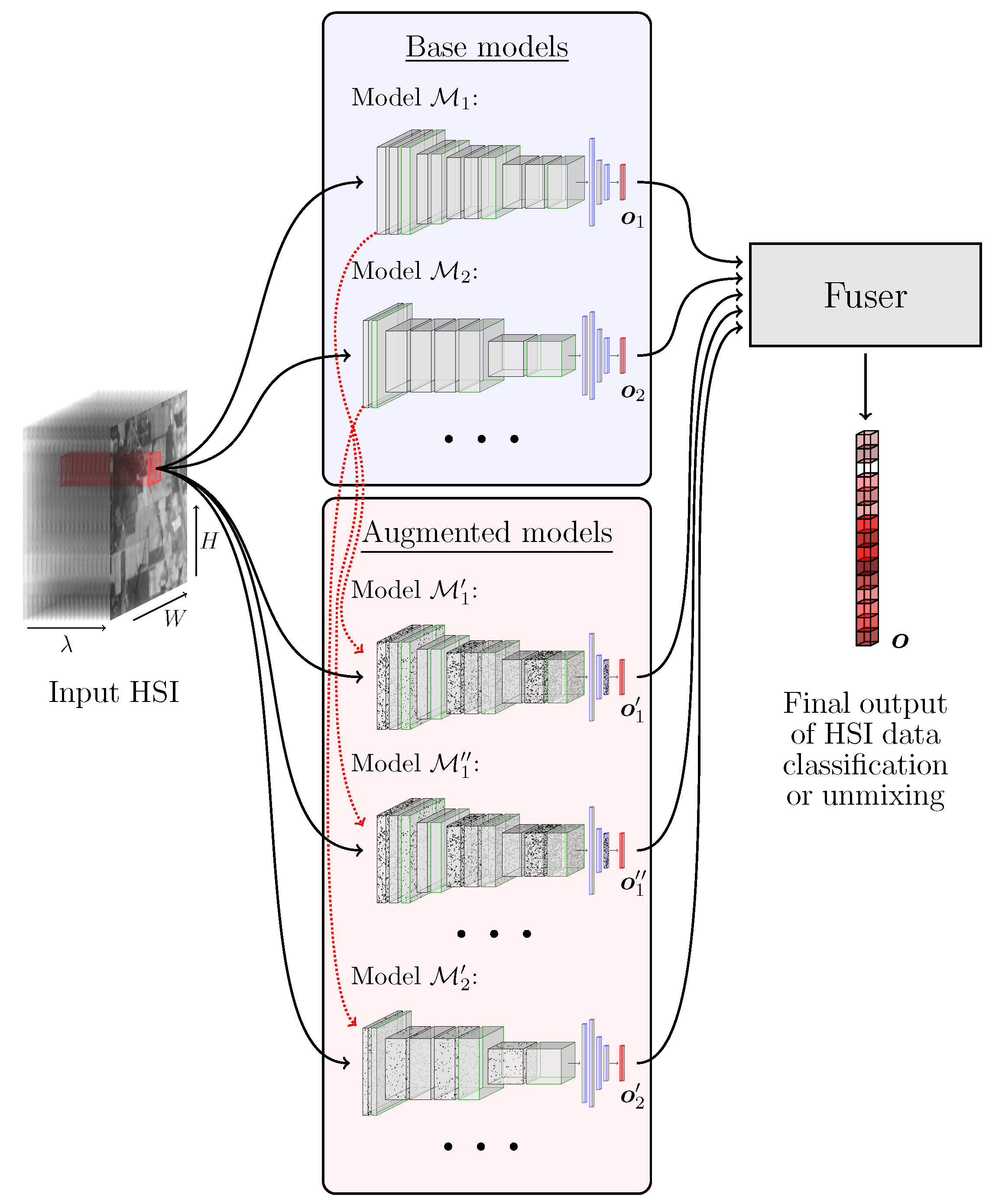
Although ensemble learning has been successfully employed in a plethora of pattern recognition tasks, its applications to the HSI analysis is under-researched, and the existent ensemble methods are focused on building HSI classifiers over different training and/or feature subsets through bootstrap aggregating [24]. To the best of our knowledge, there are no methods that combine the advantages of different deep architectures in order to improve the hyperspectral data classification or hyperspectral unmixing (HU). In this paper, we tackle this issue and propose to exploit ensemble learning for HSI analysis—a high-level visualization of our approach is rendered in Figure 1, whereas our most important contributions will be summarized in Section 1.2.

1.1. Related Work

In this section, we review the state-of-the-art of HSI classification (Section 1.1.1) and hyperspectral unmixing (Section 1.1.2) and highlight the underlying approaches exploited in the existent techniques.

1.1.1. Hyperspectral Image Data Classification

Segmentation of HSI may be approached in a pixel-wise manner without exploiting the spatial relations captured within a hyperspectral cube [25]. Hence, each pixel is classified independently based on its spectral signature—HSI segmentation thus encompasses the classification of all pixels separately. This process is often termed as HSI classification when performed in a supervised manner, even if the spatial information is exploited [26]. In many works, the HSI segmentation term is used only in the unsupervised context, where we divide an HSI into coherent regions of uniform properties. This is in contrast with the terminology adopted in the image processing community [27], where segmentation may be supervised and unsupervised, while image classification is a procedure of assigning a label (or a set of labels) to the input image based on its contents.

In general, supervised hyperspectral data classification techniques are split into classical and deep learning-based algorithms, with the former including the k-nearest neighbor classifier [28], support vector machines (SVMs) [29], Gaussian mixture models [30], and the approaches utilizing various sparse representations coupled with machine learning models [31]. Since we have been witnessing an unprecedented success of deep learning in virtually all fields of science and engineering, such algorithms are currently blooming in HSI analysis. While deep belief networks [25] and recurrent neural nets [32] effectively extract high-quality latent data representations, the use of convolutional neural networks (CNNs) allowed us to benefit either from the spectral [33], or from both spectral and spatial information captured in hyperspectral data cubes [34,35,36,37]. Recently, Okwuashi and Ndehedehe introduced a deep network combining multiple SVMs as neurons [38]. The recent advancements in the field include densely connected CNNs [39], attention mechanisms [40], and multi-branch networks [41,42] that are often of a very large capacity. However, as processing HSI on-board imaging satellites are becoming a critical real-life use case that can boost the adoption of this cutting-edge technology in practice, many attempts are aimed at elaborating lightweight models [43,44,45]. Finally, although some boosting methods couple several base models trained over different feature/training samples [24] for hyperspectral data classification, ensemble learning has not been widely researched for this task. Specifically, there are no techniques that would benefit from different approaches (spectral and spectral-spatial), or that would exploit the augmented base models generated through manipulating the weights of a trained CNN—in this paper, we follow this research pathway in order to improve the generalization of deep learners.

Deep learning has been shown successful in HSI classification and segmentation, but acquiring new representative ground-truth sets is time-consuming, costly, and human-dependent in practice [11]. The problem of limited labeled data is also reflected in the way the hyperspectral data classification methods are trained and evaluated—commonly, machine learning models are trained and tested using hyperspectral pixels sampled from the very same HSI. This approach is correct as long as there is no information leakage between the test and training samples. For the methods based on spectral features, it is sufficient to prevent the same pixel from being incorporated into the training ($\mathit{T}$) and test ($\mathsf{\Psi }$) set at the same time. However, for spectral-spatial analysis, the entire neighborhood of the pixels in the test set must be excluded from training, which has been overlooked in many works. Importantly, if it is not ensured, the estimated classification performance can easily be over-optimistic, and may not reflect the real generalization abilities of the supervised learners [33,46,47]. To effectively tackle this issue, we introduced a patch-based validation procedure, which ensures no training-test information leakage [33]—we will follow this technique in the work reported here. Furthermore, there are approaches that may be employed for (i) augmenting the existent labeled sets [48,49,50], and (ii) building classification engines in the case of very small training samples—they include transfer [51,52] and semi-supervised learning [53,54,55]. Finally, we can utilize unsupervised learning to find consistent regions within input hyperspectral scenes [56,57]. Albeit such techniques do not require ground-truth data, their results are more difficult to interpret and, hence, may not be directly applicable in real-life Earth observation (They can, however, act as a pre-segmentation step that makes generating the ground-truth labels much easier. Here, a pre-segmented HSI may be further analyzed by a human reader who would assign specific class labels to coherent regions of similar characteristics [56].).

1.1.2. Hyperspectral Unmixing

In HU, we estimate the fractional abundances of various endmembers that are captured in hyperspectral pixels, hence tackle the regression task [58,59]. In the linear HU, each pixel is a linear combination of the endmembers’ abundances. However, this assumption may be violated by changes in illuminations, variations in the atmospheric conditions, or other acquisition difficulties. Therefore, the bilinear and non-linear models have been introduced [60]. The HU algorithms may be further divided into the approaches exploiting physical modeling, mixture models, kernel methods, and artificial neural network-based techniques. In two-stage algorithms, the automated feature extraction, e.g., using auto-associative nets, is followed by fuzzy classification to perform abundance estimation [61]. There also exist very effective three-step techniques, in which the estimation of the number of endmembers in a scene is performed first, and then the identification of the spectral signatures of the endmembers, together with the estimation of the fractional abundance of each endmember in each pixel of the scene are performed (these constitute the second and the third step of this method) [62]. The majority of deep learning HU algorithms exploit CNNs (both spectral and spectral-spatial). However, due to a limited number of labeled sets, semi-supervised and unsupervised methods are also employed to tackle this task [63]. In CNNs introduced in [64], the first part of the deep architecture is a feature extractor, which encompasses several convolutional layers, whereas the final, fully-connected segment of the model estimates the abundance for each endmember in an input HSI. To prevent the model from overfitting, the dropout technique is utilized [65]. The experimental study proved that this method offers superiority to other HU approaches such as linear spectral unmixing [66] and cascaded artificial neural networks [61]. In our previous work, we investigated the influence of the training set sizes on the performance of such CNNs (and also on autoencoder-based architectures [67]) [68]. The experiments performed on two real-life datasets showed that the deterioration in the unmixing performance is especially visible for smaller training samples. Moreover, there is a training set’s cardinality threshold, over which increasing the number of training samples does not introduce improvements in HU—it may indicate that it could be possible to determine a sufficient threshold of the minimal training set size for a given task and, therefore, lower the costs of manual labeling.

In [67], a deep convolutional autoencoder (DCAE) is utilized without any prior knowledge about the abundances. However, a fully unsupervised approach should estimate both the endmembers and their abundances—DCAE exploits the linear mixing model, and employs the known endmembers’ spectra to learn the fractional abundances as a latent representation in the autoencoder part of the underlying architecture. By taking advantage of the linear model, the code extracted by the encoder is reconstructed into the input spectrum. An encoder–decoder approach was also followed in [69], where Palsson et al. exploited the encoder, which was composed of four fully-connected layers, whereas the decoder’s weights were set to the endmember spectra. The code, being the activations of the last hidden layer of the encoding part of the architecture, becomes the abundance vector for an input sample. Additionally, to enable the encoder to capture the non-linear data characteristics, it utilizes a number of non-linear activation functions, including sigmoid, rectified linear unit (ReLU) activations or leaky ReLU [70]. Furthermore, to accelerate the training phase, the batch normalization was incorporated into one of the encoder’s layers [71]. Finally, to prevent overfitting and to introduce additional regularization, a Gaussian dropout layer [65] concludes the encoding part of the model. The stacked autoencoders have been employed in [72] to improve feature extraction. Afterward, a variational autoencoder was employed for estimating the endmember signatures as well as fractional abundances. The experimental results obtained for the synthetic and real-life datasets indicated that the proposed method works on par with other state-of-the-art HU techniques. In [73], the authors suggested an interesting multitask learning architecture based on parallel autoencoders to tackle the problem of HU. Here, the spectral and spatial features are utilized to take advantage of the correlations between the neighboring pixels, where each one is fed through a separate encoder path, whereas the decoder constitutes a linear mixing model. The inputs from each path are concatenated together and connected to a hidden layer, which is shared across all encoders. This operation allows for capturing the spatial context of neighboring pixels. Finally, there have been attempts that train generative models for unsupervised unmixing, in which the endmember variability is inferred directly from the data [74].

Bhatt and Joshi summarized the most important challenges that are concerned with applying deep learning to HU [19] and indicated the lack of ground-truth datasets and restricted access to them as two major obstacles (as the remedy for that, the authors indicated transfer learning and generative models that could synthesize training data) that make the adoption of such techniques difficult in practice. Thus, building deep HU models that work well over unseen data is an open question in the literature—we tackle this problem using ensemble learning, which has not been exploited for HU so far.

1.2. Contribution

We exploit ensemble learning to improve the generalization of deep learning algorithms through benefiting from different architectural approaches to the hyperspectral data classification and unmixing. Overall, the contribution of this work is multi-fold:

• We build heterogeneous ensembles, which include spectral and spectral-spatial CNNs for hyperspectral data classification and unmixing, and propose to utilize supervised learners to benefit from the outcomes elaborated using the base models (Section 2). In our approach, their outputs are concatenated in order to form the combined feature vector, which is later fed to the fusing learner for elaborating the final answer of the ensemble. We emphasize that the proposed ensembles equipped with the supervised fusers are independent of the underlying base models and, hence, can be utilized for ensembling other, perhaps more efficient models.
• We introduce a model augmentation technique that injects Gaussian noise into weights of a trained convolutional model and show that the ensembles built with such augmented deep networks manifest better generalization abilities and outperform not only base classifiers and regression models but also other classical ensembles.
• We perform a thorough experimental validation of our approaches and confront the proposed ensembles with base models of various convolutional architectures and with other classical techniques (Section 3).
• We make our implementations publicly available at https://github.com/ESA-PhiLab/hypernet/tree/master/beetles (accessed on 18 August 2021) to ensure full reproducibility of our experimentation.

2. Methods

In this section, we present the key components of our technique. The approach for building task-agnostic ensembles is discussed in Section 2.1. Then, we present the deep architectures that are exploited as base models for hyperspectral image data classification (Section 2.2) and HU (Section 2.3).

2.1. Building Deep Ensembles

To benefit from various architectural advances in HSI analysis, we build heterogeneous ensembles containing different base models whose outcomes are fused together to elaborate the final ensemble’s decision. We exploit both classical fusers, such as the majority (hard) voting or averaging (in regression tasks), and our supervised fusing scheme. In the latter, an additional supervised model is put on top of the ensemble. It is trained over feature vectors $\mathcal{F}={[{\mathit{o}}_1;{\mathit{o}}_2;\cdots ;{\mathit{o}}_N]}^T$, where ${\mathit{o}}_i$ is the output vector of the i-th base model, and it is treated as a feature vector corresponding to ${\mathcal{M}}_i$ (see the red outputs of the base models rendered in Figure 1). The combined feature vector is fed to the fusing learner, and it includes the concatenated outputs of N base models obtained for each training sample. Therefore, the size of such feature vectors will increase for larger N’s. As an example, for a classification task, the i-th base model would elaborate c class probabilities, e.g., using the softmax layer, which would constitute ${\mathit{o}}_i$ (the size of the concatenated feature vector $\mathcal{F}$ would amount to $c·N$). On the other hand, a base regressor would elaborate the abundances for HU, and such abundance vectors would analogously be concatenated for all base models (hence, the final vector of abundances would be N times larger than a vector of abundances obtained by each base model, as it concatenates the outputs of N models). The fuser merges the base predictions and elaborates the ensemble’s output.

We not only train classification and unmixing deep models from scratch but also propose to augment the already trained base learners by injecting Gaussian noise into their weights. The probability density function p of a Gaussian variable x is

$$p\left(x\right)=\frac{1}{\sigma \sqrt{2\pi }}{e}^{-{\left(x-\mu \right)}^2/\phantom{-{\left(x-\mu \right)}^{2}2{\sigma }^2}2{\sigma }^2},$$

(1)

where $\mu$ and ${\sigma }^2$ are the mean and variance ($\sigma$ denotes standard deviation). For each j-th convolutional layer, we contaminate its weights using the Gaussian distribution with zero mean and standard deviation ${\sigma }_j^{\prime }=ϵ·{\sigma }_j^{\mathbf{w}}$, where ${\sigma }_j^{\mathbf{w}}$ is the weights’ standard deviation in the j-th layer of the corresponding i-th original model ${\mathcal{M}}_i$ (we use $ϵ=0.1$, which was experimentally selected, but fine-tuning this hyperparameter or perhaps using a set of $ϵ$ values for generating a variety of contaminated models constitute an interesting research venue that requires further investigation). Once the layers are perturbed with such Gaussian noise, we obtain the augmented model ${\mathcal{M}}_i^{\prime }$, and using this approach we can generate any number of derived learners that are included in the final ensemble together with N original models. In Figure 1, we show an example of contaminating the models ${\mathcal{M}}_1$ and ${\mathcal{M}}_2$, which results in obtaining ${\mathcal{M}}_1^{\prime }$, ${\mathcal{M}}_1^{″}$, and ${\mathcal{M}}_2^{\prime }$, whose output is further fed to the fuser, as in the case of other base models.

2.2. Hyperspectral Image Data Classification: Base Models

To verify the generalization abilities of both spectral and spectral-spatial CNNs, we investigate three convolutional architectures that are gathered in

Table 1. The CNNs for hyperspectral image data classification. We present its hyperparameters, where k denotes the number of kernels, s is stride, $\lambda$ denotes the number of hyperspectral bands, $w\times w$ is the size of the input patch, and c is the number of classes in the considered dataset. The Conv, MP, and FC are the convolutional, max-pooling, and fully-connected layers, respectively, whereas ReLU is the rectified linear unit activation function.

Model	Layer	Parameters	Activation
1D-CNN $(1\times 1\times \lambda )$	Conv1	k: $200@(1\times 1\times 6)$	ReLU
		s: $1\times 1\times 1$
	Conv2	k: $200@(1\times 1\times 6)$	ReLU
		s: $1\times 1\times 3$
	Conv3	k: $200@(1\times 1\times 6)$	ReLU
		s: $1\times 1\times 2$
	Conv4	k: $200@(1\times 1\times 6)$	ReLU
		s: $1\times 1\times 2$
	FC1	$\#\times 192$	ReLU
	FC2	$192\times 150$	ReLU
	FC3	$150\times c$	Softmax
2.5D-CNN $(w\times w\times \lambda )$	Conv1	$200@(w-3\times w-3\times \lambda )$	ReLU
	MP1	$2\times 2$
	Conv2	$200@(2\times 2\times 200)$	ReLU
	Conv3	$c@(2\times 2\times 200)$	Softmax
3D-CNN $(7\times 7\times \lambda )$	Conv1	$24@(3\times 3\times 3)$	ReLU
	Conv2	$24@(3\times 3\times 3)$	ReLU
	Conv3	$24@(3\times 3\times 3)$	ReLU
	FC1	$\#\times 512$	ReLU
	FC2	$512\times 256$	ReLU
	FC3	$256\times 128$	ReLU
	FC4	$128\times c$	Softmax

. The spectral network (referred to as 1D-CNN—this model performs the pixel-wise classification) is inspired by [33], whereas two spectral-spatial CNNs are denoted as 2.5D-CNN [36] and 3D-CNN [75] (these models perform the patch-wise classification of the central pixel in the corresponding patch, and the patch sizes for 2.5D-CNN for specific datasets were taken as suggested in [76]). Although both 2.5D-CNN and 3D-CNN models benefit from the spectral and spatial information while classifying the central pixel in an input patch, 3D-CNN can capture fine-grained spectral relations within the hyperspectral cube, as it exploits small $(3\times 3\times 3)$ convolutional kernels. It is in contrast to 2.5D-CNN whose kernels span the entire spectrum, i.e., $\lambda$ bands in the first convolutional layer.

2.3. Hyperspectral Unmixing: Base Models

For HU, we utilize the convolutional architecture introduced in [64], which can operate in both pixel- and patch-wise manner, therefore can exploit only spectral or both spectral-spatial information while elaborating the endmember abundances (

Table 2. The CNNs for HU. We report the number of kernels, alongside their dimensions, and a denotes the number of endmembers.

Variant	Layer	Parameters	Activation
1D-CNN $(1\times 1\times \lambda )$	Conv1	$3@1\times 1\times 5$	ReLU
	Conv2	$6@1\times 1\times 4$	ReLU
	Conv3	$12@1\times 1\times 5$	ReLU
	Conv4	$24@1\times 1\times 4$	ReLU
	FC1	$\#\times 192$	ReLU
	FC2	$192\times 150$	ReLU
	FC3	$150\times a$	Softmax
3D-CNN $(3\times 3\times \lambda )$	Conv1	$16@1\times 1\times 5$	ReLU
	Conv2	$32@1\times 1\times 4$	ReLU
	Conv3	$64@1\times 1\times 5$	ReLU
	Conv4	$128@1\times 1\times 4$	ReLU
	FC1	$\#\times 192$	ReLU
	FC2	$192\times 150$	ReLU
	FC3	$150\times a$	Softmax

). Here, the feature extraction part of the network (four convolutional layers) is followed by a predictor, being a multilayer perceptron with three fully-connected layers.

3. Experiments and Discussion

The experimental study is divided into two experiments, concerning hyperspectral image data classification (Section 3.1) and unmixing (Section 3.2). Here, we present the experimental settings and discuss the results in detail. Our models were coded in Python 3.6 with Tensorflow 1.12, and the experimental validation was run using an NVIDIA Tesla T4 GPU.

3.1. Hyperspectral Image Data Classification

The training (using the ADAM optimizer [77] with the categorical cross-entropy loss, and the learning rate of $0.001$, ${\beta }_1=0.9$, and ${\beta }_2=0.999$) finished if after 15 consecutive epochs the accuracy over the validation set $\mathit{V}$ ($10\%$ of randomly picked training pixels) does not increase. The hyperparameters used in the experimental validation were experimentally fine-tuned, unless stated otherwise (e.g., for the base CNNs, we pick the size of the spatial neighborhood as suggested in the corresponding papers).

To quantify the performance, we report the overall and balanced accuracy scores (OA and BA, where BA is the average of recall obtained on each class), and the values of the Cohen’s kappa $\kappa =1-\frac{1-p_o}{1-p_e}$, where $p_o$ and $p_e$ are the observed and expected agreement (assigned vs. correct label), and $-1\le \kappa \le 1$ [78] (we report $(100·\kappa )$ when we refer to $\kappa$). Since there are folds in which there are classes that were not captured within the corresponding training samples (see our training-test splits in Section 3.1.1), but they are present in the corresponding $\mathsf{\Psi }$’s, we exclude such classes from $\mathsf{\Psi }$ of a given fold (as the models were unable to learn them from $\mathit{T}$). All reported metrics are obtained for the unseen test sets $\mathsf{\Psi }$, and they are averaged across all folds (we ran training five times per fold and averaged the results).

3.1.1. Datasets

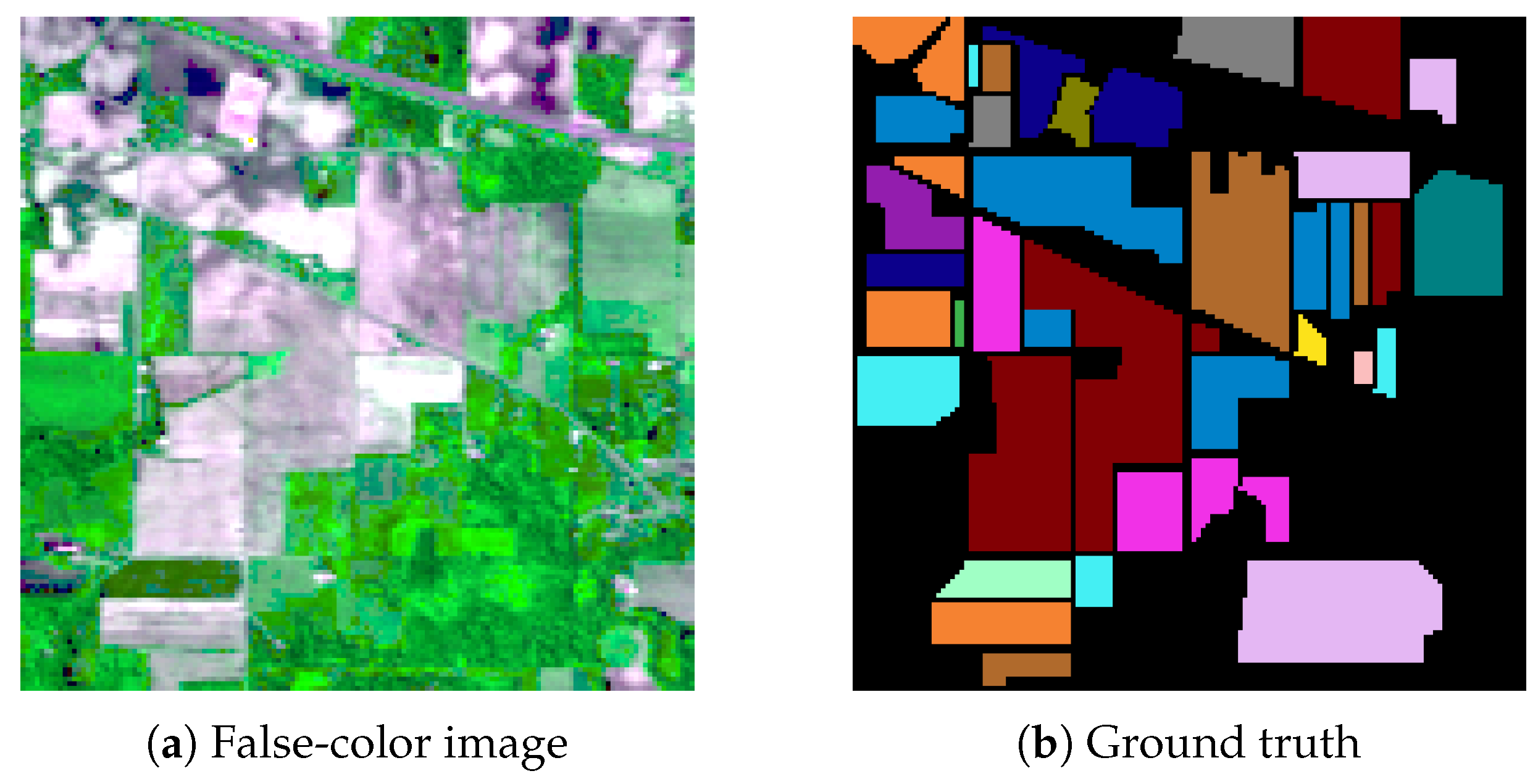
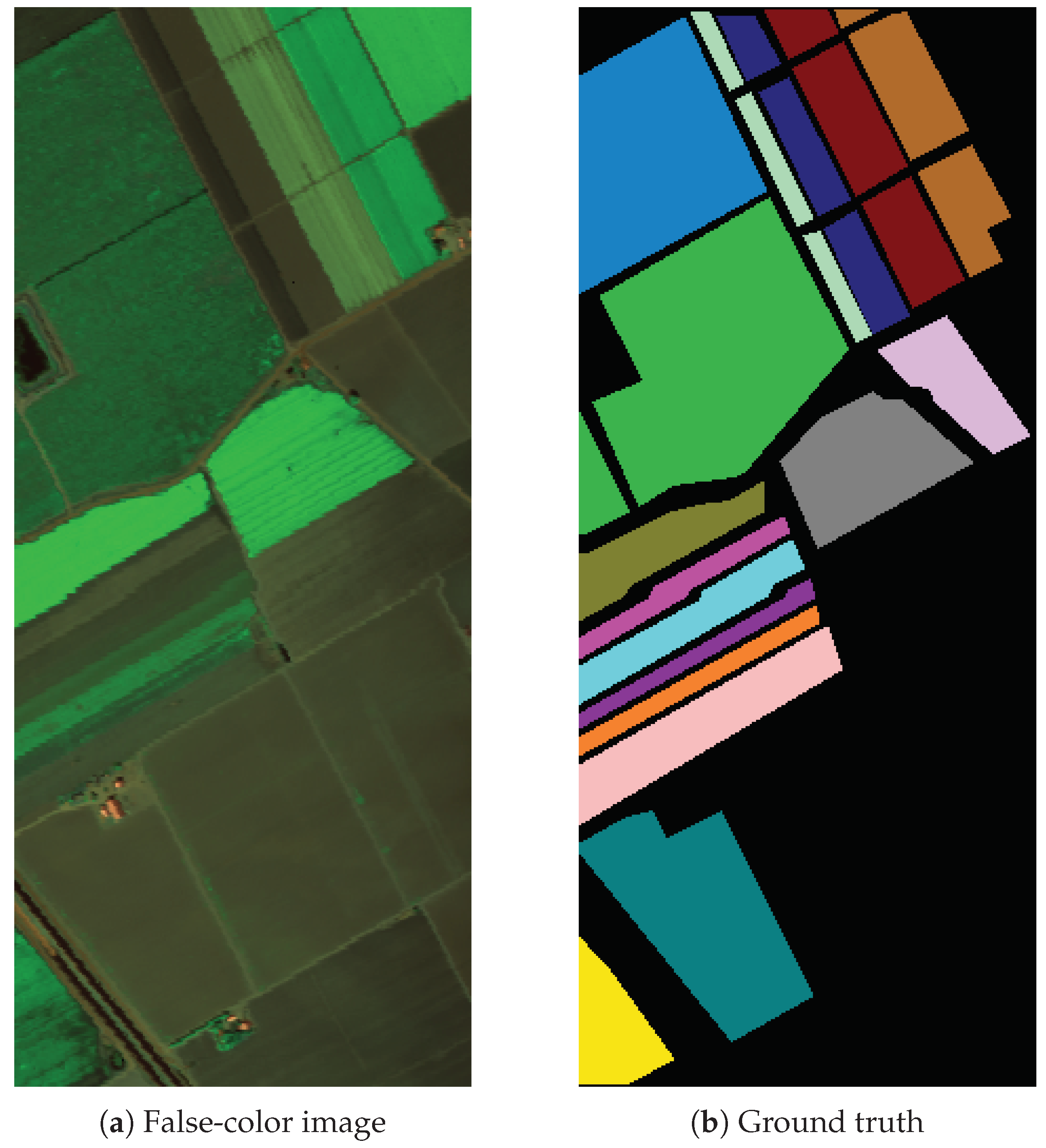
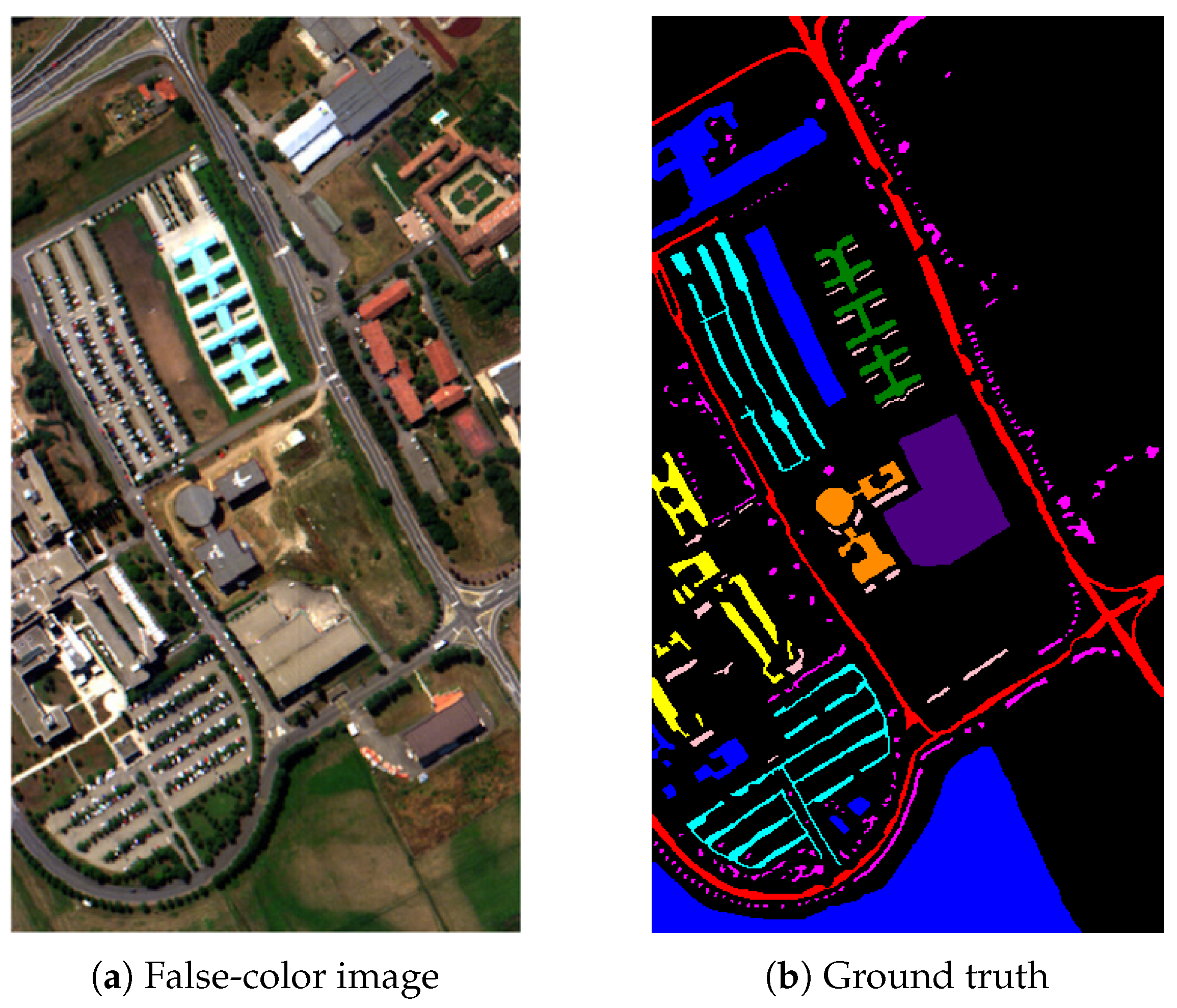
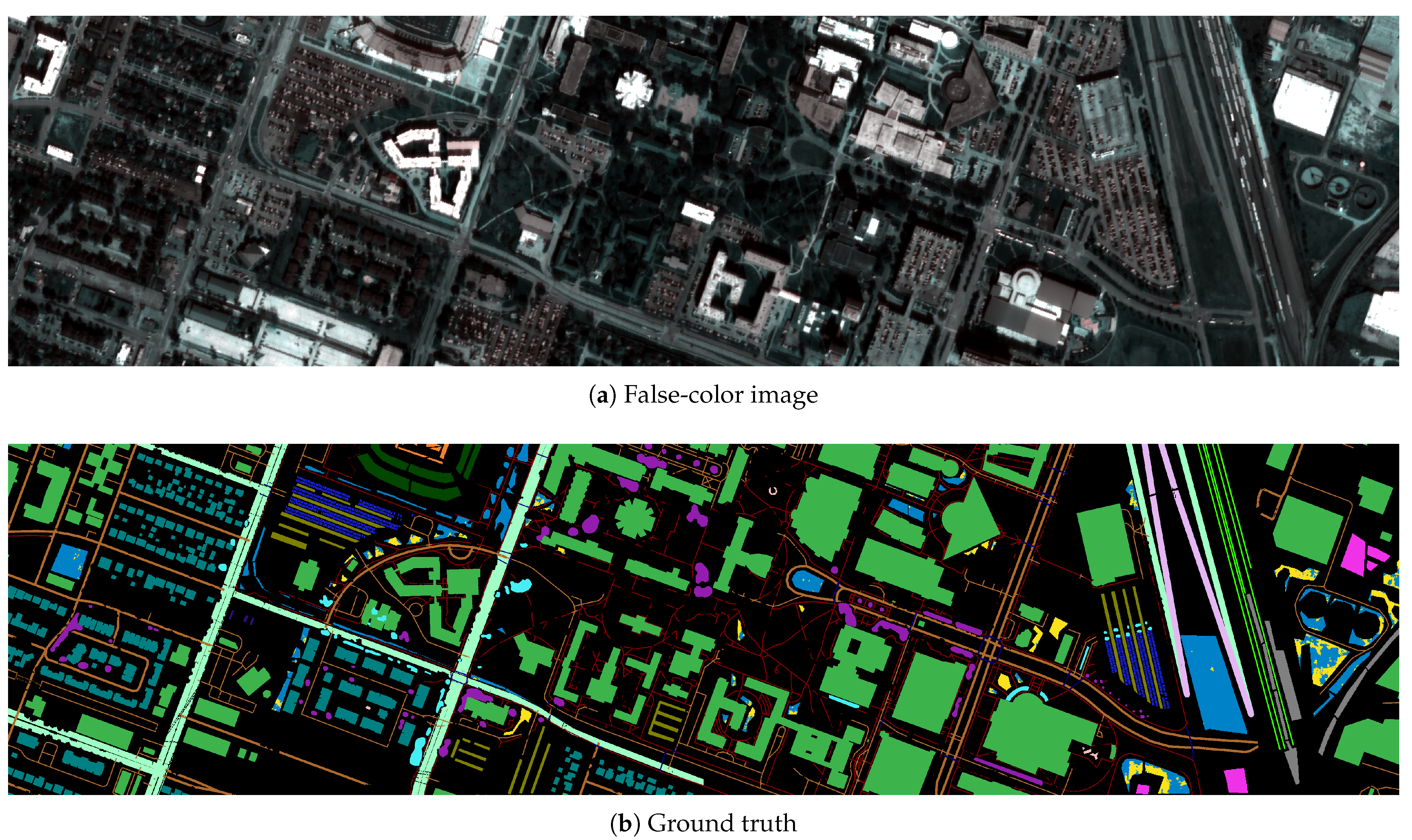
We focus on four benchmark HSIs [33]: Indian Pines (IP), Salinas Valley (SV), Pavia University (PU), and University of Houston (Houston) [79]. IP ($145\times 145$ pixels) was acquired using the Airborne Visible/Infrared Imaging Spectrometer (AVIRIS) sensor over the Indian Pines area, USA, with a spatial resolution of 20 m, and it presents agriculture, forest, and natural perennial vegetation areas (16 classes; see Figure 2 together with

Table 3. The ground-truth color, and the number of examples for each class in Indian Pines.

Class	Description	GT Color	Number of Samples
1	Alfalfa		46
2	Corn-notill		1428
3	Corn-mintill		830
4	Corn		237
5	Grass-pasture		483
6	Grass-trees		730
7	Grass-pasture-mowed		28
8	Hay-windrowed		478
9	Oats		20
10	Soybean-notill		972
11	Soybean-mintill		2455
12	Soybean-clean		593
13	Wheat		205
14	Woods		1265
15	Buildings-Grass-Trees-Drives		386
16	Stone-Steel-Towers 2		93
Total			10,249

). The number of all bands was reduced to 200 (from the original 224 bands) by the authors of this set by removing those that cover the region of water absorption. SV ($217\times 512$ pixels) was acquired over Salinas Valley, USA (with the spatial resolution of 3.7 m, capturing 204 spectral bands using the AVIRIS sensor). This set, visualized in Figure 3 and

Table 4. The ground-truth color, and the number of examples for each class in Salinas Valley.

Class	Description	GT Color	Number of Samples
1	Broccoli 1		2009
2	Broccoli 2		3726
3	Fallow 1		1976
4	Fallow 2		1394
5	Fallow 3		2678
6	Stubble		3959
7	Celery		3579
8	Grapes		11,271
9	Soil		6203
10	Corn		3278
11	Lettuce 1		1068
12	Lettuce 2		1927
13	Lettuce 3		916
14	Lettuce 4		1070
15	Vineyard 1		7268
16	Vineyard 2		1807
Total			54,129

, shows different sorts of vegetation (16 classes). PU ($340\times 610$) was captured over Pavia University, Italy (spatial resolution of 1.3 m, 103 bands, Reflective Optics System Imaging Spectrometer). It shows an urban scenery (nine classes; Figure 4 and

Table 5. The ground-truth color and number of samples for each class in Pavia University.

Class	Description	GT Color	Number of Samples
1	Asphalt		6631
2	Meadows		18,649
3	Gravel		2099
4	Trees		3064
5	Painted metal sheets		1345
6	Bare Soil		5029
7	Bitumen		1330
8	Self-Blocking Bricks		3682
9	Shadows		947
Total			42,776

). Finally, Houston ($4172\times 1202$ pixels, Figure 5 and

Table 6. The ground-truth color, and the number of examples for each class in the Houston dataset.

Class	Description	GT Color	Number of Samples
1	Healthy grass		39,196
2	Stressed grass		130,008
3	Artificial turf		2736
4	Evergreen trees		54,322
5	Deciduous trees		20,172
6	Bare earth		18,064
7	Water		1064
8	Residential buildings		158,995
9	Non-residential building		894,769
10	Roads		183,283
11	Sidewalks		136,035
12	Crosswalks		6059
13	Major thoroughfares		185,438
14	Highways		39,438
15	Railways		27,748
16	Paved parking lots		45,932
17	Unpaved parking lots		587
18	Cars		26,289
19	Trains		21,479
20	Stadium seats		27,296
Total			2,018,910

) was captured over the University of Houston campus, USA (spatial resolution of 1 m, 48 bands, ITRES CASI 1500 hyperspectral imager) and shows 20 urban land-cover/land-use classes. This set was introduced in the IEEE GRSS Data Fusion Challenge (we thank IEEE GRSS IADF and the Hyperspectral Image Analysis Lab at the University of Houston, USA).

Although Monte Carlo cross-validation has been used to verify the abilities of the HSI classification and segmentation techniques, it may lead to over-optimistic estimation of the generalization performance of deep models, especially spectral-spatial CNNs. Such deep architectures utilize all pixels in a spatial patch while classifying the central pixel, and such neighboring pixels may be included in both $\mathit{T}$ and $\mathsf{\Psi }$ [33]. To tackle this issue, we exploit the multi-fold patch-based divisions of IP, SV, and PU introduced in [33], and our two training-test split versions of Houston (referred to as Version A and B) introduced in [76]. In Version A, the $24\times 95$ patches are sampled until at least $3\times {10}^4$ training pixels are present in $\mathit{T}$. Version B divides Houston into a grid ($10\times 10$ blocks of the $120\times 477$ size), and each fold contains 20 random blocks for training. Thus, Version A includes more heterogeneously drawn patches, whereas the number of training pixels is much larger in Version B. As discussed in [76], this splitting strategy can lead to very challenging training/test samples (there might be test classes that are not captured within the corresponding training sets and, hence, the models are unable to learn them) but may also reflect practical use cases, where capturing the examples of all classes is difficult.

3.1.2. Experimental Results

The experiment is divided into two main parts—in the first one, we focus on building deep ensembles that include base CNNs of different architectures (1D-CNN, 2.5-CNN, and 3D-CNN (for brevity, we refer to these models as 1D, 2.5D, and 3D in the tables)), whereas in the second part, we investigate the impact of augmenting 1D-CNN models through our Gaussian noise injection. As the supervised fusers, we exploit a random forest (RF) with the default parameterization of 100 estimators and the Gini impurity used to measure the quality of a split, decision tree (DT), and a support vector machine (SVM) with a radial-basis kernel with $C=1$ and $\gamma =1/(\left|\mathcal{F}\right|·\mathrm{Var}\left(\mathbf{X}\right))$, where $\left|\mathcal{F}\right|$ is the number of features, and $\mathrm{Var}\left(\mathbf{X}\right)$ is the variance of the input data $\mathbf{X}$, and compare them with majority (hard) voting. Note that by using RF on top of a deep ensemble, we additionally benefit from bootstrapping, as RF builds an ensemble of DTs over different sub-samples of the training data to avoid overfitting.

Table 7. The results (BA, OA, and $\kappa$) obtained using all investigated base models and various heterogeneous ensembles built with CNNs of different architectures (with all fusing schemes: Hard, RF, DT, and SVM) for all datasets: IP, SV, PU, H(A), and H(B) (averaged across all folds and executions). The best results for each row are boldfaced, the second best results are underlined, whereas the worst are grayed.

Model→		Base Models			(1D, 2.5D, 3D)				(1D, 2.5D)				(1D, 3D)				(2.5D, 3D)
Metric↓		1D	2.5D	3D	Hard	RF	DT	SVM	Hard	RF	DT	SVM	Hard	RF	DT	SVM	Hard	RF	DT	SVM
IP	BA	66.86	40.31	46.54	43.86	48.81	52.81	57.84	56.60	60.37	55.68	60.80	53.88	61.38	55.35	59.69	52.29	57.34	45.69	47.77
	OA	68.63	48.40	52.04	50.90	54.63	59.27	63.15	60.80	64.36	62.06	65.86	60.44	65.62	60.40	64.36	59.03	62.60	52.01	54.40
	$\kappa$	64.08	40.37	45.10	44.04	48.04	53.43	57.80	55.48	59.21	56.57	60.87	54.98	60.58	54.72	59.20	52.92	57.15	45.05	47.73
SV	BA	81.39	69.98	79.31	72.03	76.88	77.52	79.18	79.67	83.99	74.82	76.72	73.75	79.93	81.04	82.96	79.79	82.08	75.46	75.97
	OA	78.01	69.60	76.46	72.93	75.45	76.86	76.70	78.41	81.16	74.08	75.20	75.10	77.00	79.07	79.61	77.03	78.85	74.87	74.72
	$\kappa$	75.17	65.74	73.43	69.34	72.26	73.80	73.66	75.50	78.71	70.74	71.97	71.73	74.02	76.36	76.95	74.04	76.09	71.59	71.41
PU	BA	80.14	77.61	76.70	76.31	80.50	80.22	81.48	77.28	80.23	79.60	80.24	78.02	80.84	78.81	80.25	80.12	81.36	79.91	80.35
	OA	79.58	78.63	76.49	79.29	80.62	80.10	80.83	79.71	79.27	79.86	80.16	81.03	80.92	78.34	79.46	80.18	81.21	79.73	80.16
	$\kappa$	72.81	70.94	68.67	71.40	73.90	73.18	74.35	72.14	72.55	72.84	73.29	73.68	74.34	71.26	72.87	73.40	74.78	72.71	73.36
H(A)	BA	47.67	38.76	38.75	39.69	38.56	37.49	37.15	35.44	38.37	38.24	36.22	35.45	40.17	37.60	35.20	40.61	39.61	38.47	39.03
	OA	59.85	52.27	51.40	54.48	52.00	49.91	51.83	53.57	51.38	50.80	51.78	53.85	53.04	50.24	50.66	55.70	53.17	50.80	52.39
	$\kappa$	47.11	38.73	37.91	40.57	38.57	36.37	38.15	37.35	37.84	37.35	38.02	37.89	39.76	36.34	36.62	41.61	39.77	37.30	38.95
H(B)	BA	47.67	49.11	52.08	50.23	49.23	50.56	52.07	53.40	52.14	47.16	46.28	51.48	52.25	50.48	50.66	54.39	52.17	50.45	51.60
	OA	59.85	62.06	62.34	64.65	62.12	62.26	63.43	66.48	62.54	60.54	62.15	66.68	63.62	61.33	62.36	66.76	63.71	62.48	63.12
	$\kappa$	47.11	50.88	52.00	53.79	51.07	51.61	53.19	56.29	52.25	49.05	50.98	56.16	53.38	50.71	51.96	56.70	53.47	51.93	52.66

gathers the results obtained for all datasets (averaged across all folds and runs) using the heterogeneous deep ensembles. We can observe that the spectral 1D-CNN model consistently elaborates accurate classification scores and significantly outperforms both 2.5D-CNN and 3D-CNN. We can attribute it to the fact that the amount and representativeness of training samples are very limited, hence large-capacity learners tend to overfit and do not generalize well over the unseen data. Conversely, if the training sets are larger, as in the case of Houston (ver. B), which is referred to as H(B) in Table 7, a spectral-spatial 3D-CNN model gave notably better results than 1D-CNN. Therefore, it was able to capture fine-grained characteristics of the underlying classes manifested in both spatial pixel’s neighborhood and spectral pixel’s information. The problem of limited number of training samples can be, however, tackled using a variety of techniques, including transfer learning and data augmentation through using the Extended Multi-attribute Profiles—this approach was shown to be successful in land cover classification for a decreased number of hyperspectral bands [80].

The results show that including 1D-CNN effectively compensates for the lack of generalization abilities of spectral-spatial models. It may be especially useful in emerging use cases, in which quantifying the capabilities of deep networks over large unseen test samples is difficult or even impossible, as the amount of annotated data is very limited. In such situations, we can benefit from different deep architectural choices—on the one hand, ensembling high-quality spectral-spatial models (i.e., those delivering accurate classification), e.g., 3D-CNN for Houston (ver. B) with 1D-CNN or 2.5D-CNN would improve its performance even further (see the SVM fuser in an ensemble containing three models). On the other hand, low-quality CNNs are significantly boosted with those that generalize well (see all ensembles that include 1D-CNN). Additionally, we can observe that the supervised fusers notably outperformed hard voting in the majority of cases (according to the two-tailed Wilcoxon test over per-class accuracies at $p<0.05$). The only exception here, being DT and SVM for the ensemble of 2.5D-CNN and 3D-CNN models, shows that the training sample, built with the outputs of base spectral-spatial CNNs, was not representative enough (and presumably low-quality) to train effective fusers. In the hard voting case, if the models elaborate different predictions in ensembles with two CNNs, we select the prediction with the lower uncertainty. It indicates that the uncertain predictions adversely affect the performance of the supervised fusers, especially DT and SVM, and pruning such uncertain base models from the ensembles could help improve their capabilities independently from the fusing scheme.

In

Table 8. The results (BA, OA, and $\kappa$) obtained using a single 1D-CNN model (1D), and using the ensembles with different numbers of augmented 1D-CNNs (# copies) with all fusing schemes (Hard, RF, DT, and SVM)—each ensemble always contains one original 1D-CNN model. We report the results for all datasets: IP, SV, PU, H(A), and H(B). Note that the augmented models were generated by injecting noise into the weights of the original model, and the number of such contaminated (augmented) copies may be freely updated. The best results for each row are boldfaced, the second best are underlined, whereas the worst are grayed.

# Copies→			1 Copy				2 Copies				4 Copies				8 Copies				16 Copies
Metric↓		1D	Hard	RF	DT	SVM	Hard	RF	DT	SVM	Hard	RF	DT	SVM	Hard	RF	DT	SVM	Hard	RF	DT	SVM
IP	BA	66.86	63.48	68.58	66.08	67.48	64.51	68.50	66.67	67.61	62.59	68.41	65.63	67.41	60.84	68.47	67.05	66.54	60.67	68.66	67.37	66.90
	OA	68.63	64.72	70.39	66.68	69.81	65.67	70.42	67.28	69.67	63.90	70.50	67.16	69.69	63.06	70.37	67.12	69.58	63.14	70.38	67.02	69.65
	$\kappa$	64.08	59.69	66.31	61.94	65.41	60.55	66.36	62.55	65.24	58.48	66.46	62.40	65.25	57.62	66.32	62.44	65.12	57.73	66.34	62.31	65.19
SV	BA	81.39	79.64	82.80	82.46	83.54	81.11	82.71	83.23	83.61	81.08	82.89	83.46	83.90	80.51	82.83	83.06	83.83	80.51	82.95	82.15	83.87
	OA	78.01	77.53	79.52	78.46	79.48	78.22	79.53	79.54	79.56	78.21	79.72	79.55	80.36	77.64	79.50	79.56	80.35	77.68	79.58	78.58	80.07
	$\kappa$	75.17	74.55	76.92	75.72	76.88	75.38	76.93	76.92	76.97	75.36	77.14	76.91	77.82	74.73	76.91	76.93	77.81	74.77	76.99	75.85	77.52
PU	BA	80.14	79.61	79.82	79.67	80.71	80.01	79.82	80.04	80.81	80.05	79.81	79.91	80.92	80.11	79.62	79.82	80.93	80.19	79.69	79.74	80.91
	OA	79.58	79.43	78.68	78.57	80.42	79.10	78.74	79.03	80.45	79.02	78.72	78.25	80.45	78.93	78.70	78.36	80.46	78.94	78.70	78.11	80.40
	$\kappa$	72.81	72.51	71.85	71.64	73.88	72.29	71.92	72.21	73.92	72.21	71.89	71.33	73.93	72.12	71.84	71.29	73.95	72.15	71.86	71.12	73.88
H(A)	BA	47.67	47.86	45.25	45.10	47.79	47.90	45.16	45.41	47.89	47.92	45.08	45.22	48.07	47.80	45.07	44.84	48.04	47.69	45.12	44.45	47.99
	OA	59.85	60.47	57.50	56.99	59.50	59.95	57.47	57.25	59.55	60.05	57.40	57.21	59.71	60.16	57.38	57.04	59.85	60.23	57.40	56.91	59.83
	$\kappa$	47.11	47.71	44.49	43.43	46.80	47.27	44.46	43.79	46.85	47.37	44.39	43.69	47.11	47.42	44.38	43.50	47.24	47.40	44.38	43.38	47.20
H(B)	BA	47.67	55.01	54.38	54.60	56.95	56.06	54.22	54.44	57.03	56.15	54.18	54.14	57.26	56.20	54.14	54.40	57.41	56.29	54.16	54.68	57.52
	OA	59.85	65.93	64.47	64.35	66.51	65.73	64.36	64.32	66.69	65.69	64.25	64.32	66.80	66.03	64.24	64.30	66.90	66.05	64.15	64.33	66.97
	$\kappa$	47.11	56.08	54.77	54.26	56.99	56.07	54.67	54.20	57.10	56.10	54.57	54.22	57.25	56.47	54.57	54.18	57.40	56.46	54.49	54.25	57.58

, we present the results obtained using the deep ensembles that contain different numbers of augmented 1D-CNN models (we focus on 1D-CNN, as it obtains the best classification across all base learners). Such augmented models are generated by injecting Gaussian noise into the original (uncontaminated) model (as rendered in Figure 1)—here, any number of augmented models may be elaborated based on a single (original) model. Introducing augmented models helps to significantly improve the ensemble’s generalization, and SVM fusers consistently outperformed the other schemes (note that the hard voting approach gave the worst scores in all cases). Therefore, such noisy CNNs can be treated as a model-level regularization. It is also manifested in

Table 9. The ranking obtained for all investigated HSI classification methods, averaged across all datasets (the best algorithm for a given set receives the ranking of 1, the second best: 2, and so on). We consider $\kappa$ to be the primary metric and, hence, sort the algorithms according to rankings obtained for $\kappa$. We report the rankings for the (i) heterogeneus deep ensembles built with different CNNs (see the detailed results in Table 7), (ii) augmented ensembles containing various numbers of noise-contaminated 1D-CNN (Table 8), and (iii) all methods altogether.

Ensemble	Fuser	BA	OA	$\mathit{\kappa }$
Heterogeneous	RF (2.5D, 3D)	4.2	4.6	4.2
	RF (1D, 3D)	3.4	5.4	5.0
	Hard (2.5D, 3D)	6.8	5.8	5.8
	...	...	...	...
	DT (1D, 2.5D)	13.6	13.8	13.6
	DT (2.5D, 3D)	13.4	13.6	14.6
	2.5D	15.4	16.0	15.8
Augmented	SVM (4 copies)	3.0	4.4	4.2
	SVM (8 copies)	4.4	4.2	4.2
	SVM (16 copies)	4.0	5.2	4.8
	...	...	...	...
	DT (4 copies)	13.6	15	16.2
	DT (1 copy)	15.4	16.6	17
	DT (16 copies)	14.6	17.2	17.6
All	SVM (4 copies)	3.6	5.6	5.0
	SVM (8 copies)	5.0	5.4	5.0
	SVM (16 copies)	4.6	6.4	5.8
	...	...	...	...
	DT (1D, 3D)	33.6	30.6	30.2
	3D	31.4	34.2	33.4
	2.5D	35.4	35.2	35.8

, where we collect the rankings of all investigated methods, calculated separately for ensembles containing 1D-CNN, 2.5-CNN, and 3D-CNN models (Heterogeneous), those with augmented 1D-CNNs (Augmented), and collectively for all approaches (All). Here, the rankings are averaged over all datasets, and the best-performing technique for a given set obtains the ranking of 1, the second best: 2, and so forth (therefore, the smaller the value of the ranking becomes, the better the corresponding algorithm is). We consider $\kappa$ to be the primary metric, hence sort the algorithms according to rankings obtained for $\kappa$. The results show that augmenting 1D-CNNs through manipulating their weights can lead to the best generalization over unseen data—the top three models included the deep ensembles with the SVM fusers containing different numbers of augmented 1D-CNNs.

The training times obtained for all investigated base models indicate that performing the convolutions through the spectral dimension notably slows down the process (

Table 10. Training time (in seconds) of all investigated base models, for all datasets.

Dataset	1D-CNN	2.5D-CNN	3D-CNN
IP	13.28	2.84	39.16
SV	14.33	14.25	64.33
PU	7.44	5.11	22.07
H(A)	41.31	27.44	87.33
H(B)	261.57	323.16	538.89

). To build the ensembles with the proposed fusers, such supervised learners must be trained over the elaborated outputs of base models—their training time depends on the selected fusing scheme (

Table 11. Training time (in seconds) of all investigated supervised fusers: RF, DT, SVM, for all datasets: IP, SV, PU, H(A) and H(B), obtained for the ensembles with different numbers of augmented 1D-CNNs (# copies). Each ensemble always contains one original 1D-CNN model.

# Copies→	1 Copy			2 Copies			4 Copies			8 Copies			16 Copies
Dataset	RF	DT	SVM	RF	DT	SVM	RF	DT	SVM	RF	DT	SVM	RF	DT	SVM
IP	15.55	138.50	530.00	13.70	128.00	182.75	13.15	417.75	651.25	17.20	528.25	1214.00	28.15	179.00	1184.75
SV	18.04	177.40	175.80	19.92	166.80	166.60	24.68	445.20	185.80	31.60	147.40	316.40	47.56	177.60	330.20
PU	12.92	136.60	122.40	14.12	123.40	133.00	15.24	152.60	83.60	17.76	127.40	204.80	27.68	101.40	182.40
H(A)	510.48	122.80	428.40	525.76	129.80	529.00	560.72	148.20	726.40	851.32	181.20	1104.00	897.68	346.60	1921.40
H(B)	951.00	160.80	6164.60	1031.04	191.20	8969.40	1256.40	253.40	98,723.34	1509.88	358.60	108,325.67	2018.48	631.60	128,238.24

). We can observe that the training is the slowest for the SVM fuser, as it has cubic time complexity with respect to the training set size (therefore, the training process is the most time-consuming for the largest datasets, H(A) and H(B), being two versions of the Houston scene). Similarly, in the case of the heterogeneous ensembles in which we use the base models of various architectures, the training time of the fusers depends on the number of exploited models (

Table 12. Training time (in seconds) of all investigated supervised fusers: RF, DT, SVM, for all datasets: IP, SV, PU, H(A) and H(B), obtained for the ensembles with different CNN architectures (various combinations of the 1D, 2.5D, and 3D models).

Ensemble→	(1D, 2.5D, 3D)			(1D, 2.5D)			(1D, 3D)			(2.5D, 3D)
Dataset	RF	DT	SVM	RF	DT	SVM	RF	DT	SVM	RF	DT	SVM
IP	67.25	43.65	45.15	56.10	37.40	36.45	48.70	40.70	40.40	41.70	38.80	35.85
SV	96.00	64.48	60.20	258.68	49.80	49.04	66.88	49.68	49.68	65.92	56.48	55.28
PU	72.12	42.32	39.92	49.72	35.32	35.48	54.72	37.40	37.60	47.52	39.00	39.80
H(A)	240.96	139.20	206.88	259.88	115.12	323.48	424.96	115.72	191.84	471.12	286.04	417.36
H(B)	466.80	132.92	947.24	480.52	142.80	2142.32	621.80	177.84	1910.12	687.84	283.48	1380.80

). Additionally, assembling different base models into ensembles will result in building different feature spaces (as their outcomes form feature vectors)—it may also affect the training time, as the convergence of the supervised training of specific classifiers/regressors can vary [81]. Therefore, incorporating an additional feature selection step in our pipeline could not only help improve the capabilities of the ensembles (through rejecting the least informative or redundant features) but could also reduce the training time of their fusers—it constitutes an interesting research area, which should be further explored.

To better understand the operational abilities of the models, we report the prediction (test) times of the ensembles with different numbers of augmented 1D-CNNs (

Table 13. Prediction time (in seconds, over the entire test set) of all investigated supervised fusers: RF, DT, SVM (together with the Hard voting), for all datasets: IP, SV, PU, H(A) and H(B), obtained for the ensembles with different numbers of augmented 1D-CNNs (# copies). Each ensemble always contains one original 1D-CNN model.

# Copies→	1 Copy				2 Copies				4 Copies				8 Copies				16 Copies
Dataset	Hard	RF	DT	SVM	Hard	RF	DT	SVM	Hard	RF	DT	SVM	Hard	RF	DT	SVM	Hard	RF	DT	SVM
IP	1.17	1.16	1.17	1.46	2.14	1.30	1.29	1.66	4.53	1.61	1.59	2.12	6.88	2.20	2.18	3.07	9.37	3.39	3.37	4.96
SV	3.59	7.00	3.47	5.62	4.62	8.13	4.44	7.16	6.82	10.04	6.40	10.38	11.34	14.38	10.37	16.61	21.59	22.34	18.23	29.37
PU	2.13	2.37	3.20	2.91	2.58	2.73	2.41	2.75	3.48	3.51	3.09	3.55	5.48	5.00	4.41	5.07	10.37	7.95	6.73	9.04
H(A)	55.65	468.63	17.81	322.48	61.62	478.32	24.63	421.66	78.88	508.47	40.25	616.14	111.01	790.50	68.99	988.35	177.04	816.69	132.52	1792.90
H(B)	43.90	429.58	14.24	299.82	50.67	430.78	20.52	402.75	62.55	447.03	32.93	601.32	89.92	515.02	57.86	902.82	144.31	677.53	108.55	1582.83

), together with the prediction times obtained using the ensembles built with base models of various CNN architectures (

Table 14. Prediction time (in seconds, over the entire test set) of all investigated supervised fusers: RF, DT, SVM (together with the Hard voting), for all datasets: IP, SV, PU, H(A) and H(B), obtained for the ensembles with different CNN architectures (various combinations of the 1D, 2.5D, and 3D models).

	(1D, 2.5D, 3D)				(1D, 2.5D)				(1D, 3D)				(2.5D, 3D)
Dataset	Hard	RF	DT	SVM	Hard	RF	DT	SVM	Hard	RF	DT	SVM	Hard	RF	DT	SVM
IP	0.15	0.08	<0.01	0.19	0.15	0.08	<0.01	0.18	0.15	0.08	<0.01	0.17	0.15	0.08	<0.01	0.21
SV	0.94	0.40	0.01	1.00	0.93	0.39	<0.01	0.91	0.97	0.39	<0.01	1.10	0.92	0.38	0.01	0.77
PU	0.75	0.19	<0.01	0.12	0.77	0.20	<0.01	0.12	0.80	0.20	<0.01	0.13	0.75	0.19	<0.01	0.08
H(A)	39.56	26.77	0.37	175.20	38.33	27.40	0.29	204.19	38.74	25.50	0.30	214.04	38.48	26.68	0.29	116.00
H(B)	32.49	31.63	0.36	176.23	32.05	28.60	0.34	198.39	30.99	28.01	0.30	211.85	31.43	28.11	0.31	109.93

). Here, the increase in the inference time strongly depends on the selected fuser (see, e.g., a minor impact of the increasing number of contaminated 1D-CNNs on the operation of the ensemble with RF in Table 13, and a much more visible impact of this increase once the SVM fuser is utilized). Although the inference time is increased for ensembles when compared to the base models (the test time, averaged for all datasets amounted to 2.88, 15.80, and 21.78 s for the 1D-CNN, 2.5D-CNN, and 3D-CNN models, respectively), the proposed techniques can still maintain very fast operation while significantly improving the accuracy of the classification engine. Note that, as in the case of the training time, the inference time is dependent on a specific supervised fuser. As an example, the SVM fusers trained over the outcomes of the 1D, 2.5D, and 3D models would likely include a different number of support vectors (being the selected training vectors determining the position of the decision hyperplane) than the SVMs trained over the outputs of the 1D and 3D models (due to different underlying feature spaces). If the number of support vectors was smaller in the former case, the inference time of the fuser would be shorter even though the number of base models is larger, because the prediction time linearly depends on the number of support vectors in the case of SVMs [82].

3.2. Hyperspectral Unmixing

In our experimental study, we exploit the original hyperparameters of the investigated models [64,67] and, hence, the neighborhood of the $3\times 3$ size is utilized for 3D-CNN. For comparison, we use the DCAE architecture (

Table 15. The DCAE architecture. We report the number of kernels, alongside their dimensions.

Variant	Layer	Parameters	Activation
1D-DCAE $(1\times 1\times \lambda )$	Conv1	$2@1\times 1\times 3$	ReLU
	Conv2	$4@1\times 1\times 3$	ReLU
	Conv3	$8@1\times 1\times 3$	ReLU
	Conv4	$16@1\times 1\times 3$	ReLU
	Conv5	$32@1\times 1\times 3$	ReLU
	FC1	$\#\times 256$	ReLU
	FC2	$256\times a$	+Softmax
	FC3	$a\times \lambda$	ReLU
3D-DCAE $(5\times 5\times \lambda )$	Conv1	$16@3\times 3\times 3$	ReLU
	Conv2	$32@3\times 3\times 3$	ReLU
	Conv3	$64@1\times 1\times 3$	ReLU
	Conv4	$128@1\times 1\times 3$	ReLU
	FC1	$\#\times 256$	ReLU
	FC2	$256\times a$	+Softmax
	FC3	$a\times \lambda$	ReLU

) with originally proposed hyperparameters (the spatial neighborhood of $5\times 5$ for 3D-DCAE), and we exploit a single FC layer as a decoder, where the weight matrix is set to the endmembers’ spectral characteristics (similarly, it can work with separate pixels or patches, and these variants are referred to as 1D-DCAE and 3D-DCAE). It is built upon the observation that the input pixel can be represented as a linear combination of its abundances, and the endmembers’ matrix is built with the spectral characteristics of the materials captured in an HSI [67]. The latent vector obtained by the encoder, therefore, explains the vector of endmember abundances. Since DCAE is trained in an unsupervised way, such base models cannot be fit into our ensemble that exploits a supervised learner as a fuser, but we investigate the abilities of deep unsupervised ensembles that couple DCAEs trained over different training samples through averaging their outcomes. Additionally, the classical hyperspectral data unmixing techniques, including support vector regression (R-SVR) and the fully constrained least-squares based linear unmixing (LMM) models were taken for comparison (with the experimentally fine-tuned parameterization).

Both models were trained using Adam with the learning rates of ${10}^{-3}$, ${10}^{-4}$, ${10}^{-5}$, and $5\times {10}^{-5}$ for the pixel-based and cube-based variants of CNN and DCAE, respectively. The maximum number of epochs was 100, with the early stopping of 15 epochs without an improvement in the loss value over a random $\mathit{V}$ ($10\%$ of all training pixels)—the aforementioned hyperparameters were experimentally fine-tuned. To minimize the distance between the input and reconstructed sample in both variants of DCAE, we utilize the spectral information divergence (SID) as the loss function [83] (a standard mean square error loss is exploited to train the unmixing CNNs).

We perform 30-fold Monte Carlo cross-validation, and sample 30 test sets that do not change with the change of the training set size (as in the HSI classification experiment, we report the results obtained for $\mathsf{\Psi }$’s). The test set size is kept constant as suggested in [64]. For the Jasper and Urban set (see Section 3.2.1), we have $7.5\times {10}^3$ and $47\times {10}^3$ training pixels in total. To verify the impact of the training set size on the unmixing ensembles including different base models, we sample approximately $\{1,6,13,33,66\}\%$ random training pixels and form reduced sets of $\{75,500,{10}^3,2.5\times {10}^3,5\times {10}^3\}$ and $\{470,2.8\times {10}^3,6.1\times {10}^3,15.5\times {10}^3,31\times {10}^3\}$ pixels for Jasper and Urban, respectively. To measure the performance of unmixing algorithms, we use the metrics that quantify the distance between the estimated and observed abundances (the lower values these metrics have, the better corresponding unmixing becomes): the root-mean square error (RMSE), and the root-mean square abundance angle distance (rmsAAD). The RMSE is:

$$\mathrm{RMSE}=\sqrt{\frac{{\sum }_{i=1}^{\left|\mathsf{\Psi }\right|}{(a_i-{\widehat{a}}_i)}^2}{\left|\mathsf{\Psi }\right|}},$$

(2)

where $\left|\mathsf{\Psi }\right|$ denotes the number of samples in $\mathsf{\Psi }$, whereas a and $\widehat{a}$ represent the observed and estimated abundance vectors. Additionally, the rmsAAD becomes:

$$\mathrm{rmsAAD}=\sqrt{\frac{{\sum }_{i=1}^{\left|\mathsf{\Psi }\right|}arccos{\left(\frac{a_i^{\top }{\widehat{a}}_i}{\parallel a_i\parallel \parallel {\widehat{a}}_i\parallel }\right)}^2}{\left|\mathsf{\Psi }\right|}}.$$

(3)

3.2.1. Datasets

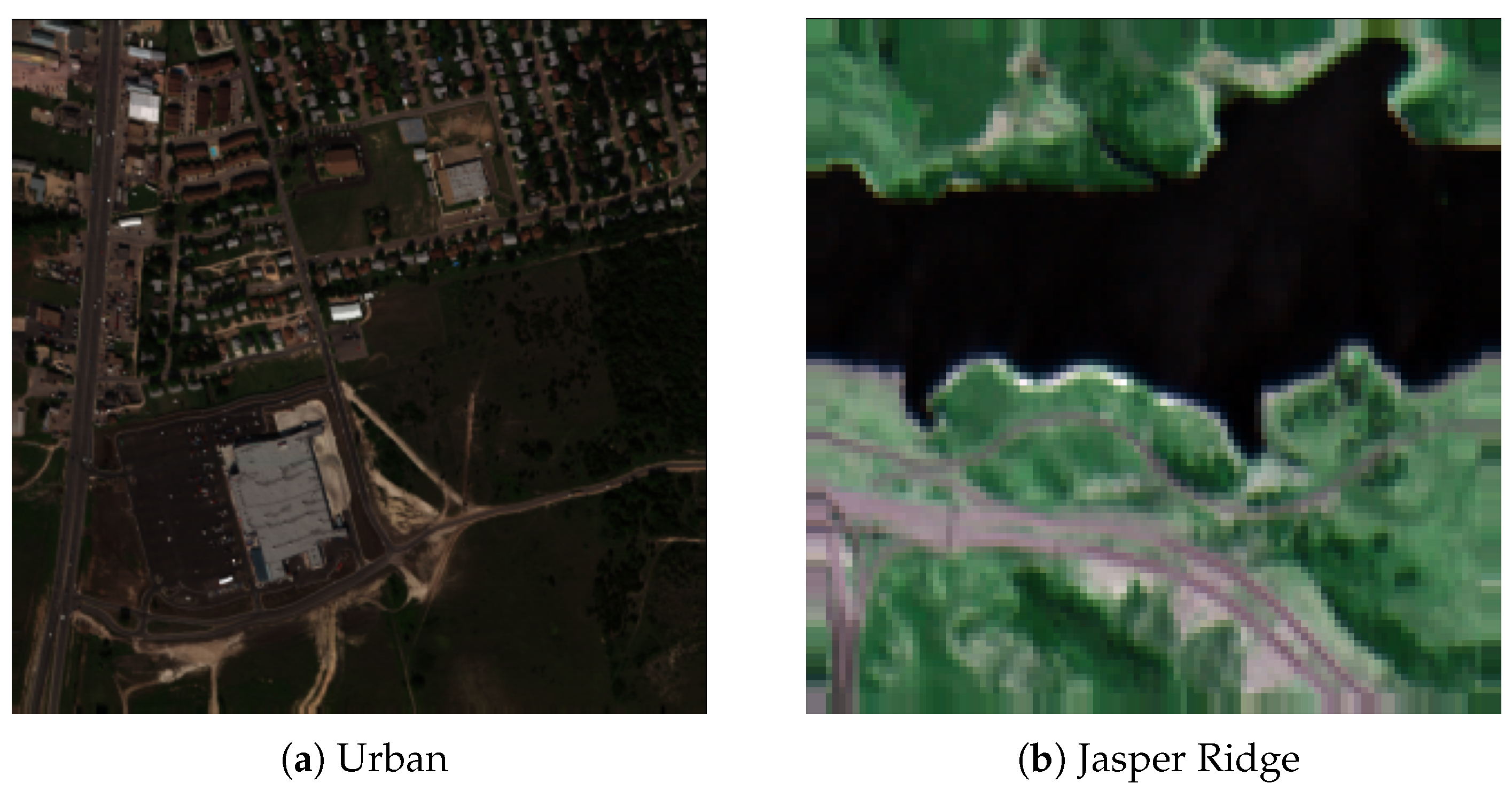
We focus on two HU benchmarks (Figure 6): Urban (Ur) and Jasper Ridge (JR) [84]. In Urban ($207\times 307$, 162 bands), we have three versions of the ground truth with four, five, and six endmembers. We utilize the most challenging variant with six endmembers: #1 Asphalt, #2 Grass, #3 Tree, #4 Roof, #5 Metal, and #6 Dirt. The JR dataset ($100\times 100$, 198 hyperspectral channels out of 224 original bands, as the ones contaminated by water vapor and atmospheric effects were removed by the authors of this set) includes four endmembers: #1 Road, #2 Water, #3 Soil, and #4 Tree.

3.2.2. Experimental Results

We not only investigate the impact of introducing augmented models into the ensembles but also analyze the ensembles containing the models trained over training sets of different sizes. As the supervised fusers, we use a random forest regressor (RF) with 100 estimators and the mean squared error used to measure the split’s quality, decision tree (DT), and a support vector regressor (SVR) with a radial-basis kernel (with the same parameterization as in Section 3.1.2).

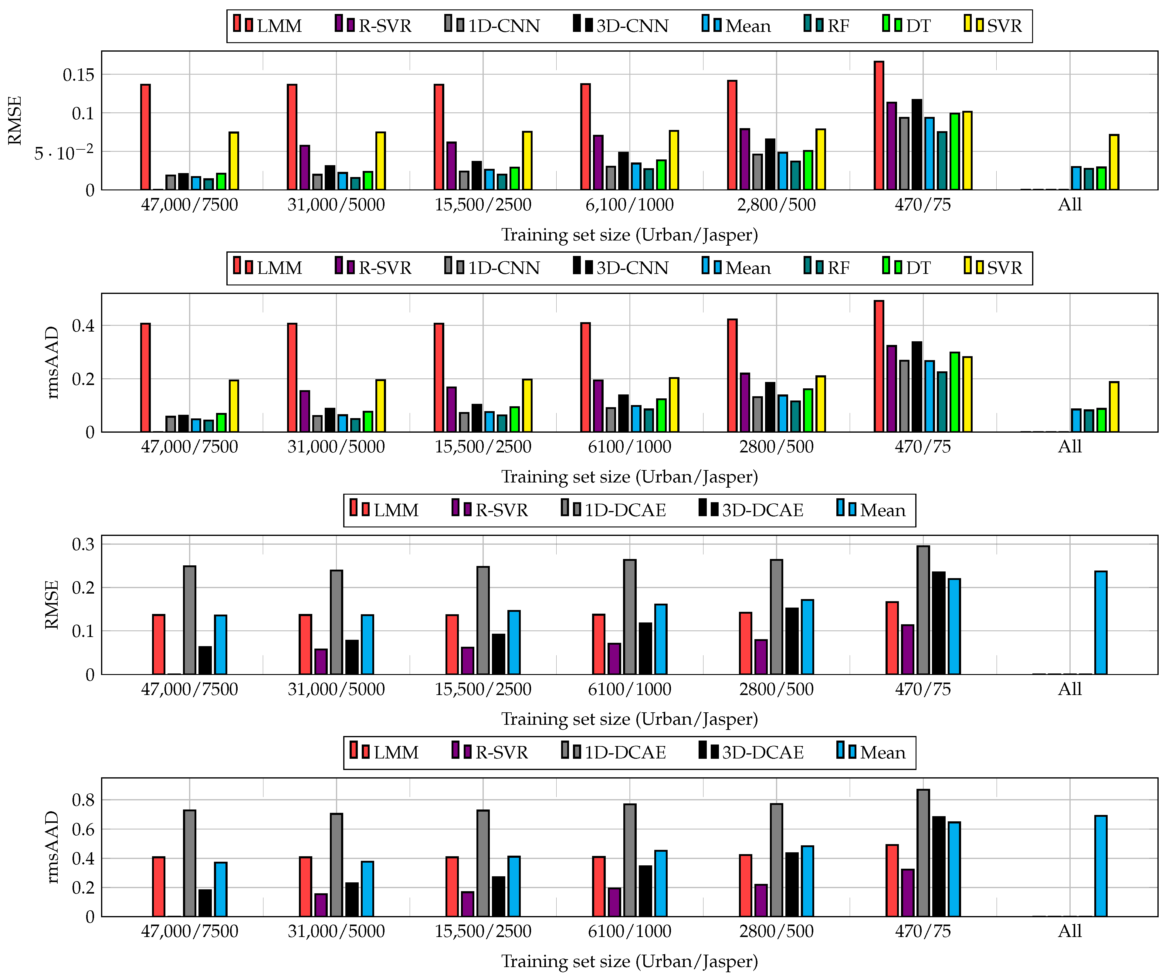
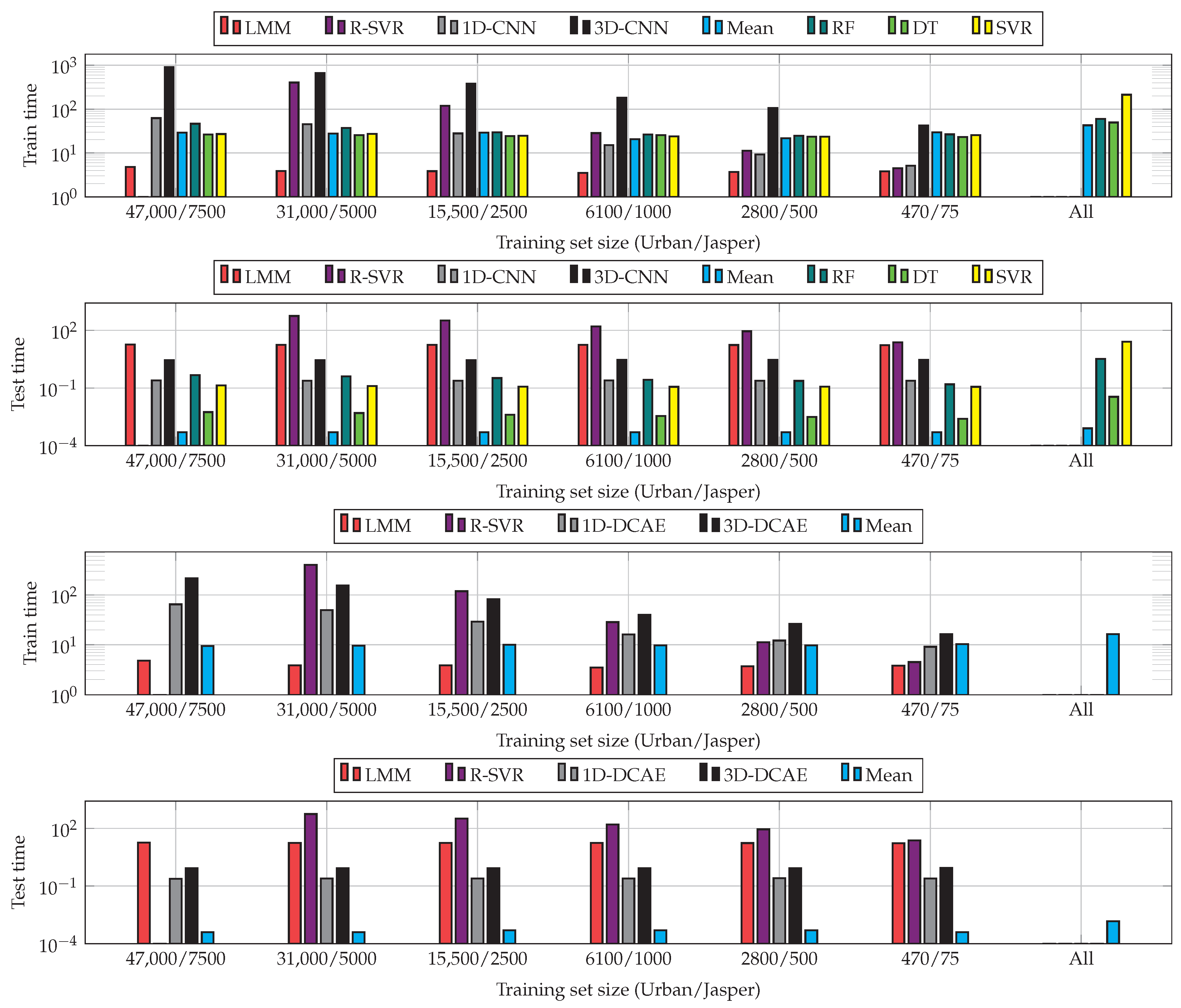
The results obtained for all sizes of training sets and algorithms are visualized in Figure 7. Although increasing the training samples helps enhance the abilities of CNNs and DCAEs, we can observe very little improvements for the largest $\mathit{T}$’s (see the results obtained for the entire training sets and 66% random examples). Building heterogeneous ensembles allows us to improve the unmixing process for all $\mathit{T}$’s, with the RF fuser outperforming the others. As SVR does not natively support multi-target regression, we fit one regressor per target to support the multi-target unmixing task. This technique, however, does not exploit the inter-target relations and resulted in the worst performance in the majority of cases. Finally, the models trained using larger $\mathit{T}$’s (in the All variant of our deep ensembles) effectively compensated for low-quality models trained from limited ground-truth samples. Additionally, the results show that the suggested ensembles are able to outperform the classical hyperspectral data unmixing techniques (note that the results are not reported for the largest training set in the case of R-SVR, as this regressor failed to train within the assumed time budget of 12 h). In Figure 8, we can appreciate the training and test times obtained for all investigated unmixing procedures and averaged for both datasets (as already mentioned, the R-SVR results are not reported, as it failed to train within 12 h). It is worth mentioning that the ensemble approach has a minor influence on the non-functional capabilities of the algorithms and, hence, allows us to maintain fast inference (significantly faster than, e.g., R-SVR).

Table 16. The results obtained using a single 1D-CNN model (1D) and using the ensembles with different numbers of augmented 1D-CNNs (# copies) with all fusers (Mean, RF, DT, and SVR); each ensemble always contains one original 1D-CNN. Note that the augmented models were generated by injecting noise into the weights of the original model, and the number of such contaminated (augmented) copies may be freely updated. We report the results for both datasets: Ur and JR. The best results for each row are bold, the second best are underlined, and the worst are grayed. We multiplied RMSE and rmsAAD by 100.

# Copies→			1 Copy				2 Copies				4 Copies				8 Copies				16 Copies
	Metric↓	1D	Mean	RF	DT	SVR	Mean	RF	DT	SVR	Mean	RF	DT	SVR	Mean	RF	DT	SVR	Mean	RF	DT	SVR
Ur	RMSE	6.76	8.26	6.58	8.47	9.46	8.11	6.55	8.50	9.41	8.31	6.48	8.46	9.35	8.12	6.43	8.42	9.31	8.23	6.40	8.54	9.27
	rmsAAD	23.63	27.67	23.81	30.44	30.27	27.17	23.73	30.57	30.12	27.49	23.52	30.39	29.97	26.71	23.32	30.22	29.85	26.87	23.22	30.71	29.74
JR	RMSE	11.95	12.58	9.79	11.72	12.20	12.45	9.56	11.72	12.02	12.73	9.46	11.57	11.97	12.78	9.40	11.56	11.96	12.92	9.25	11.66	11.88
	rmsAAD	29.88	31.46	25.00	30.11	30.00	31.07	24.49	30.22	29.52	31.73	24.18	29.79	29.36	31.63	24.07	29.84	29.33	31.87	23.72	30.18	29.17

gathers the results obtained using the deep ensembles with noise-augmented 1D-CNN models trained over 1% of available training pixels (note that the metrics are multiplied by 100). Since DCAE in an unsupervised learner, generating the augmented DCAEs would unlikely improve its operational abilities, as we cannot exploit supervised fusers to aggregate the original and perturbed models’ predictions. The issue of augmenting and ensembling unsupervised models therefore, requires, further research attention—our preliminary experiments showed that averaging the predictions (the mean ensemble) of the original and augmented 1D-DCAEs did not result in visible improvements. As in HSI classification, introducing perturbed models significantly boosted the generalization capabilities of 1D-CNNs for both datasets and enabled us to elaborate well-generalizing ensembles based on very weak learners. It indicates that ensemble learning backed up with our model augmentation may help accelerate the adoption of CNN unmixing models for emerging use cases, in which the amount of ground-truth data is small and obtaining new training samples is costly or infeasible in practice. Our previous observations concerning the training and inference times of the proposed ensembles are confirmed in

Table 17. Training and prediction (test) times (in seconds, the test times are reported for the entire test sets) for the investigated ensembles containing a given number of 1D-CNN copies (# copies), for all supervised fusers (RF, DT, and SVR, together with the mean fusion), and for a single 1D-CNN (1D).

# Copies→			1 Copy				2 Copies				4 Copies				8 Copies				16 Copies
	Time.↓	1D	Mean	RF	DT	SVR	Mean	RF	DT	SVR	Mean	RF	DT	SVR	Mean	RF	DT	SVR	Mean	RF	DT	SVR
Ur	Train	6.21	4.20	5.89	5.58	9.87	4.56	5.25	4.79	4.86	5.09	6.12	5.99	5.63	20.29	8.43	8.21	7.72	12.19	16.83	14.44	13.95
	Test	0.39	0.37	0.56	0.26	0.55	0.57	0.69	0.40	0.75	0.97	0.94	0.64	1.17	1.98	1.49	1.18	2.03	5.06	2.48	2.27	3.81
JR	Train	4.01	3.60	3.94	4.52	4.95	3.89	4.65	4.80	5.61	4.57	5.65	4.97	5.82	6.16	7.13	7.95	6.98	10.03	13.66	13.22	12.99
	Test	0.09	0.15	0.06	0.04	0.04	0.22	0.07	0.05	0.05	0.40	0.08	0.06	0.08	0.90	0.12	0.10	0.11	2.93	0.19	0.16	0.17

—delivering the prediction over unseen test sets remains very fast for various numbers of contaminated 1D-CNN models included in the unmixing ensemble. It indicates that one can improve the quality of HU by building such ensembles while minimally affecting the non-functional capabilities of the algorithms.

4. Conclusions

Deep learning approaches have become an established tool in both hyperspectral image data classification and unmixing, but the lack of ground-truth data is an important obstacle, which hampers the adoption of such large-capacity learners and makes their generalization abilities questionable in practical applications. We introduced the deep ensembles for HSI analysis that not only benefit from different deep architectural advances capturing spectral and spectral-spatial characteristics within the input HSI but also from supervised learners acting as efficient fusers of base models. Additionally, we introduced the model augmentation technique, which allows us to synthesize deep models by injecting noise into the original network’s weights. The experiments performed for HSI classification and unmixing indicated that our deep ensembles coupled with supervised fusers significantly outperform base learners and classical fusing schemes (and also the classical techniques for hyperspectral data unmixing), and the model augmentation approach notably boosts the ensembles’ generalization over the unseen test data. It is worth mentioning that the suggested ensemble approaches are independent of the underlying base models, hence including other, perhaps more efficient state-of-the-art deep architectures (for both hyperspectral data classification and unmixing), could help further improve their operational capabilities.

The research reported in this paper constitutes an interesting departure point for further research in hyperspectral image analysis using ensemble learning. In the work reported here, we suggested building ensembles that can benefit from either exploiting various architectural advances (if the convolutional neural networks are utilized), or from the models that are perturbed through the noise contamination of their weights. However, the problem of selecting appropriate base models to form the final ensemble needs further investigation, as rejecting low-quality models could be beneficial in this context [23]. Furthermore, it might be useful to increase the impact of the original (uncontaminated) model on the final output of the ensemble, by either increasing the number of copies of this model or appropriately weighting its output in the fusing scheme. Addressing these issues could ultimately lead us to fully-automated and data-driven techniques capable of automatically elaborating well-generalizing ensemble models for specific hyperspectral image analysis tasks. As the amount of labeled training data (especially hyperspectral image data) is commonly limited in emerging use cases, ensuring the high-quality classification and unmixing performance of large capacity supervised learners (e.g., 3D CNNs) is of high practical importance, as such models are able to capture fine-grained spectral and spatial features. Here, several possible approaches exist, and they include—among others—effective data augmentation [49,80] or transfer learning [85,86]. Finally, developing lightweight models that could be efficiently run on-board satellites in hardware-constrained execution environments is currently attracting research and industry attention [87,88], because it could allow us to process highly-dimensional hyperspectral imaging in orbit; therefore, it would be possible to transfer the results of this processing back to Earth, rather than raw image data. It, in turn, would increase the practical utility of such imagery by delivering specific value from the image data much faster.

References

- Kruse, F. Identification and mapping of minerals in drill core using hyperspectral image analysis of infrared reflectance spectra. Int. J. Remote Sens. 1996, 17, 1623–1632. [Google Scholar] [CrossRef]
- Govender, M.; Chetty, K.; Bulcock, H. A review of hyperspectral remote sensing and its application in vegetation and water resource studies. Water SA 2007, 33, 145–151. [Google Scholar] [CrossRef] [Green Version]
- Lu, G.; Fei, B. Medical hyperspectral imaging: A review. J. Biomed. Opt. 2014, 19, 010901. [Google Scholar] [CrossRef] [PubMed]
- Warren, R.E.; Cohn, D.B. Chemical detection on surfaces by hyperspectral imaging. J. Appl. Remote Sens. 2017, 11, 1–16. [Google Scholar] [CrossRef] [Green Version]
- Edelman, G.; Gaston, E.; Van Leeuwen, T.; Cullen, P.; Aalders, M. Hyperspectral imaging for non-contact analysis of forensic traces. Forensic Sci. Int. 2012, 223, 28–39. [Google Scholar] [CrossRef] [Green Version]
- Khan, M.J.; Khan, H.S.; Yousaf, A.; Khurshid, K.; Abbas, A. Modern trends in hyperspectral image analysis: A review. IEEE Access 2018, 6, 14118–14129. [Google Scholar] [CrossRef]
- Dou, X.; Li, C.; Shi, Q.; Liu, M. Super-Resolution for Hyperspectral Remote Sensing Images Based on the 3D Attention-SRGAN Network. Remote Sens. 2020, 12, 1204. [Google Scholar] [CrossRef] [Green Version]
- Dong, Y.; Du, B.; Zhang, L.; Hu, X. Hyperspectral Target Detection via Adaptive Information—Theoretic Metric Learning with Local Constraints. Remote Sens. 2018, 10, 1415. [Google Scholar] [CrossRef] [Green Version]
- Dong, Y.; Du, B.; Zhang, L.; Zhang, L. Exploring Locally Adaptive Dimensionality Reduction for Hyperspectral Image Classification: A Maximum Margin Metric Learning Aspect. IEEE J. Sel. Top. Appl. Earth Obs. Remote Sens. 2017, 10, 1136–1150. [Google Scholar] [CrossRef]
- Dong, Y.; Du, B.; Zhang, L.; Zhang, L. Dimensionality Reduction and Classification of Hyperspectral Images Using Ensemble Discriminative Local Metric Learning. IEEE Trans. Geosci. Remote Sens. 2017, 55, 2509–2524. [Google Scholar] [CrossRef]
- Zhou, X.; Prasad, S. Advances in Deep Learning for Hyperspectral Image Analysis–Addressing Challenges Arising in Practical Imaging Scenarios. In Hyperspectral Image Analysis; Springer: Berlin/Heidelberg, Germany, 2020; pp. 117–140. [Google Scholar]
- Jia, S.; Jiang, S.; Lin, Z.; Li, N.; Xu, M.; Yu, S. A survey: Deep learning for hyperspectral image classification with few labeled samples. Neurocomputing 2021, 448, 179–204. [Google Scholar] [CrossRef]
- Luo, F.; Zhang, L.; Du, B.; Zhang, L. Dimensionality Reduction With Enhanced Hybrid-Graph Discriminant Learning for Hyperspectral Image Classification. IEEE Trans. Geosci. Remote Sens. 2020, 58, 5336–5353. [Google Scholar] [CrossRef]
- Song, W.; Li, S.; Fang, L.; Lu, T. Hyperspectral Image Classification With Deep Feature Fusion Network. IEEE Trans. Geosci. Remote Sens. 2018, 56, 3173–3184. [Google Scholar] [CrossRef]
- Xiong, F.; Zhou, J.; Qian, Y. Material Based Object Tracking in Hyperspectral Videos. IEEE Trans. Image Process. 2020, 29, 3719–3733. [Google Scholar] [CrossRef]
- Winkens, C.; Sattler, F.; Adams, V.; Paulus, D. HyKo: A Spectral Dataset for Scene Understanding. In Proceedings of the IEEE International Conference on Computer Vision Workshops (ICCVW), Venice, Italy, 22–29 October 2017; pp. 254–261. [Google Scholar] [CrossRef]
- Liu, S.; Marinelli, D.; Bruzzone, L.; Bovolo, F. A Review of Change Detection in Multitemporal Hyperspectral Images: Current Techniques, Applications, and Challenges. IEEE Geosci. Remote Sens. Mag. 2019, 7, 140–158. [Google Scholar] [CrossRef]
- Zhang, J.; Rivard, B.; Sánchez-Azofeifa, A.; Castro-Esau, K. Intra- and inter-class spectral variability of tropical tree species at La Selva, Costa Rica: Implications for species identification using HYDICE imagery. Remote Sens. Environ. 2006, 105, 129–141. [Google Scholar] [CrossRef]
- Bhatt, J.S.; Joshi, M. Deep Learning in Hyperspectral Unmixing: A Review. In Proceedings of the IEEE International Geoscience and Remote Sensing Symposium, Waikoloa, HI, USA, 26 September–2 October 2020; pp. 2189–2192. [Google Scholar]
- He, B.; Lakshminarayanan, B.; Teh, Y.W. Bayesian Deep Ensembles via the Neural Tangent Kernel. In Proceedings of the 2020 Conference on Neural Information Processing Systems, Virtual, 6–12 December 2020. [Google Scholar]
- Woźniak, M.; Graña, M.; Corchado, E. A survey of multiple classifier systems as hybrid systems. Inf. Fusion 2014, 16, 3–17. [Google Scholar] [CrossRef] [Green Version]
- Cruz, R.M.O.; Hafemann, L.G.; Sabourin, R.; Cavalcanti, G.D.C. DESlib: A Dynamic ensemble selection library in Python. J. Mach. Learn. Res. 2020, 21, 1–5. [Google Scholar]
- Kardas, A.; Kawulok, M.; Nalepa, J. On Evolutionary Classification Ensembles. In Proceedings of the 2019 IEEE Congress on Evolutionary Computation (CEC), Wellington, New Zealand, 10–13 June 2019; pp. 2974–2981. [Google Scholar]
- Su, H.; Yu, Y.; Du, Q.; Du, P. Ensemble Learning for Hyperspectral Image Classification Using Tangent Collaborative Representation. IEEE Trans. Geosci. Remote Sens. 2020, 58, 3778–3790. [Google Scholar] [CrossRef]
- Zhong, P.; Gong, Z.; Li, S.; Schönlieb, C.B. Learning to Diversify Deep Belief Networks for Hyperspectral Image Classification. IEEE Trans. Geosci. Remote Sens. 2017, 55, 3516–3530. [Google Scholar] [CrossRef]
- Imani, M.; Ghassemian, H. An overview on spectral and spatial information fusion for hyperspectral image classification: Current trends and challenges. Inf. Fusion 2020, 59, 59–83. [Google Scholar] [CrossRef]
- Belgiu, M.; Drǎguţ, L. Comparing supervised and unsupervised multiresolution segmentation approaches for extracting buildings from very high resolution imagery. ISPRS J. Photogramm. Remote Sens. 2014, 96, 67–75. [Google Scholar] [CrossRef] [PubMed] [Green Version]
- Ma, L.; Crawford, M.M.; Tian, J. Local manifold learning-based k-nearest-neighbor for hyperspectral image classification. IEEE Trans. Geosci. Remote Sens. 2010, 48, 4099–4109. [Google Scholar] [CrossRef]
- Archibald, R.; Fann, G. Feature selection and classification of hyperspectral images with support vector machines. IEEE Geosci. Remote Sens. Lett. 2007, 4, 674–677. [Google Scholar] [CrossRef]
- Prasad, S.; Li, W.; Fowler, J.E.; Bruce, L.M. Information fusion in the redundant-wavelet-transform domain for noise-robust hyperspectral classification. IEEE TGRS 2012, 50, 3474–3486. [Google Scholar] [CrossRef]
- Li, C.; Ma, Y.; Mei, X.; Liu, C.; Ma, J. Hyperspectral image classification with robust sparse representation. IEEE Geosci. Remote Sens. Lett. 2016, 13, 641–645. [Google Scholar] [CrossRef]
- Mou, L.; Ghamisi, P.; Zhu, X.X. Deep Recurrent Neural Networks for Hyperspectral Classification. IEEE Trans. Geosci. Remote Sens. 2017, 55, 3639–3655. [Google Scholar] [CrossRef] [Green Version]
- Nalepa, J.; Myller, M.; Kawulok, M. Validating Hyperspectral Image Segmentation. IEEE Geosci. Remote Sens. Lett. 2019, 16, 1264–1268. [Google Scholar] [CrossRef] [Green Version]
- Zhao, W.; Du, S. Spectral-Spatial Feature Extraction for Hyperspectral Image Classification. IEEE Trans. Geosci. Remote Sens. 2016, 54, 4544–4554. [Google Scholar] [CrossRef]
- Santara, A.; Mani, K.; Hatwar, P.; Singh, A.; Garg, A.; Padia, K.; Mitra, P. BASS Net: Band-Adaptive Spectral-Spatial Feature Learning Neural Network for Hyperspectral Image Classification. IEEE Trans. Geosci. Remote Sens. 2017, 55, 5293–5301. [Google Scholar] [CrossRef] [Green Version]
- Gao, Q.; Lim, S.; Jia, X. Hyperspectral Image Classification Using Convolutional Neural Networks and Multiple Feature Learning. Remote Sens. 2018, 10, 299. [Google Scholar] [CrossRef] [Green Version]
- Paoletti, M.E.; Haut, J.M.; Plaza, J.; Plaza, A. Deep learning classifiers for hyperspectral imaging: A review. ISPRS J. Photogramm. Remote Sens. 2019, 158, 279–317. [Google Scholar] [CrossRef]
- Okwuashi, O.; Ndehedehe, C.E. Deep support vector machine for hyperspectral image classification. Pattern Recognit. 2020, 103, 107298. [Google Scholar] [CrossRef]
- Li, G.; Zhang, C.; Lei, R.; Zhang, X.; Ye, Z.; Li, X. Hyperspectral remote sensing image classification using three-dimensional-squeeze-and-excitation-DenseNet (3D-SE-DenseNet). Remote Sens. Lett. 2020, 11, 195–203. [Google Scholar] [CrossRef]
- Li, R.; Zheng, S.; Duan, C.; Yang, Y.; Wang, X. Classification of hyperspectral image based on double-branch dual-attention mechanism network. Remote Sens. 2020, 12, 582. [Google Scholar] [CrossRef] [Green Version]
- Sun, G.; Zhang, X.; Jia, X.; Ren, J.; Zhang, A.; Yao, Y.; Zhao, H. Deep fusion of localized spectral features and multi-scale spatial features for effective classification of hyperspectral images. Int. J. Appl. Earth Obs. Geoinf. 2020, 91, 102157. [Google Scholar] [CrossRef]
- Qu, L.; Zhu, X.; Zheng, J.; Zou, L. Triple-Attention-Based Parallel Network for Hyperspectral Image Classification. Remote Sens. 2021, 13, 324. [Google Scholar] [CrossRef]
- Li, R.; Duan, C. Litedensenet: A lightweight network for hyperspectral image classification. arXiv 2020, arXiv:2004.08112. [Google Scholar]
- Han, K.; Wang, Y.; Tian, Q.; Guo, J.; Xu, C.; Xu, C. Ghostnet: More features from cheap operations. In Proceedings of the IEEE/CVF Conference on Computer Vision and Pattern Recognition, Seattle, WA, USA, 16–18 January 2020; pp. 1580–1589. [Google Scholar]
- Paoletti, M.E.; Haut, J.M.; Pereira, N.S.; Plaza, J.; Plaza, A. Ghostnet for Hyperspectral Image Classification. IEEE Trans. Geosci. Remote Sens. 2021, 1–16. [Google Scholar] [CrossRef]
- Liang, J.; Zhou, J.; Qian, Y.; Wen, L.; Bai, X.; Gao, Y. On the sampling strategy for evaluation of spectral-spatial methods in hyperspectral image classification. IEEE Trans. Geosci. Remote Sens. 2016, 55, 862–880. [Google Scholar] [CrossRef] [Green Version]
- Zhao, J.; Ge, Y.; Cao, X. Non-overlapping classification of hyperspectral imagery. Remote Sens. Lett. 2019, 10, 968–977. [Google Scholar] [CrossRef]
- Feng, J.; Chen, J.; Liu, L.; Cao, X.; Zhang, X.; Jiao, L.; Yu, T. CNN-based multilayer spatial–spectral feature fusion and sample augmentation with local and nonlocal constraints for hyperspectral image classification. IEEE J. Sel. Top. Appl. Earth Obs. Remote Sens. 2019, 12, 1299–1313. [Google Scholar] [CrossRef]
- Haut, J.M.; Paoletti, M.E.; Plaza, J.; Plaza, A.; Li, J. Hyperspectral image classification using random occlusion data augmentation. IEEE Geosci. Remote Sens. Lett. 2019, 16, 1751–1755. [Google Scholar] [CrossRef]
- Nalepa, J.; Myller, M.; Kawulok, M. Training-and test-time data augmentation for hyperspectral image segmentation. IEEE Geosci. Remote Sens. Lett. 2020, 17, 292–296. [Google Scholar] [CrossRef]
- Marmanis, D.; Datcu, M.; Esch, T.; Stilla, U. Deep learning earth observation classification using ImageNet pretrained networks. IEEE Geosci. Remote Sens. Lett. 2015, 13, 105–109. [Google Scholar] [CrossRef] [Green Version]
- Nalepa, J.; Myller, M.; Kawulok, M. Transfer learning for segmenting dimensionally reduced hyperspectral images. IEEE Geosci. Remote Sens. Lett. 2020, 17, 1228–1232. [Google Scholar] [CrossRef] [Green Version]
- Liu, H.; Cocea, M. Semi-random partitioning of data into training and test sets in granular computing context. Granul. Comput. 2017, 2, 357–386. [Google Scholar] [CrossRef] [Green Version]
- Li, F.; Clausi, D.; Xu, L.; Wong, A. ST-IRGS: A Region-Based Self-Training Algorithm Applied to Hyperspectral Image Classification and Segmentation. IEEE Trans. Geosci. Remote Sens. 2018, 56, 3–16. [Google Scholar] [CrossRef]
- Zhang, Y.; Liu, K.; Dong, Y.; Wu, K.; Hu, X. Semisupervised Classification Based on SLIC Segmentation for Hyperspectral Image. IEEE Geosci. Remote Sens. Lett. 2020, 17, 1440–1444. [Google Scholar] [CrossRef]
- Nalepa, J.; Myller, M.; Imai, Y.; Honda, K.I.; Takeda, T.; Antoniak, M. Unsupervised segmentation of hyperspectral images using 3-D convolutional autoencoders. IEEE Geosci. Remote Sens. Lett. 2020, 17, 1948–1952. [Google Scholar] [CrossRef]
- Tulczyjew, L.; Kawulok, M.; Nalepa, J. Unsupervised Feature Learning Using Recurrent Neural Nets for Segmenting Hyperspectral Images. IEEE Geosci. Remote Sens. Lett. 2020. [Google Scholar] [CrossRef]
- Xu, X.; Li, J.; Li, S.; Plaza, A. Generalized Morphological Component Analysis for Hyperspectral Unmixing. IEEE Trans. Geosci. Remote Sens. 2020, 58, 2817–2832. [Google Scholar] [CrossRef]
- Su, Y.; Xu, X.; Li, J.; Qi, H.; Gamba, P.; Plaza, A. Deep Autoencoders with Multitask Learning for Bilinear Hyperspectral Unmixing. IEEE Trans. Geosci. Remote Sens. 2021, 59, 8615–8629. [Google Scholar] [CrossRef]
- Heylen, R.; Parente, M.; Gader, P. A Review of Nonlinear Hyperspectral Unmixing Methods. IEEE J. Sel. Top. Appl. Earth Obs. Remote Sens. 2014, 7, 1844–1868. [Google Scholar] [CrossRef]
- Licciardi, G.A.; Del Frate, F. Pixel Unmixing in Hyperspectral Data by Means of Neural Networks. IEEE Trans. Geosci. Remote Sens. 2011, 49, 4163–4172. [Google Scholar] [CrossRef]
- Li, J.; Bioucas-Dias, J.M.; Plaza, A.; Liu, L. Robust Collaborative Nonnegative Matrix Factorization for Hyperspectral Unmixing. IEEE Trans. Geosci. Remote Sens. 2016, 54, 6076–6090. [Google Scholar] [CrossRef] [Green Version]
- Koirala, B.; Scheunders, P. A Semi-Supervised Method for Nonlinear Hyperspectral Unmixing. In Proceedings of the IEEE International Geoscience and Remote Sensing Symposium, Yokohama, Japan, 28 July–2 August 2019; pp. 361–364. [Google Scholar]
- Zhang, X.; Sun, Y.; Zhang, J.; Wu, P.; Jiao, L. Hyperspectral Unmixing via Deep Convolutional Neural Networks. IEEE Geosci. Remote Sens. Lett. 2018, 15, 1755–1759. [Google Scholar] [CrossRef]
- Srivastava, N.; Hinton, G.; Krizhevsky, A.; Sutskever, I.; Salakhutdinov, R. Dropout: A simple way to prevent neural networks from overfitting. J. Mach. Learn. Res. 2014, 15, 1929–1958. [Google Scholar]
- Bioucas-Dias, J.M.; Plaza, A.; Dobigeon, N.; Parente, M.; Du, Q.; Gader, P.; Chanussot, J. Hyperspectral unmixing overview: Geometrical, statistical, and sparse regression-based approaches. IEEE J. Sel. Top. Appl. Earth Obs. Remote Sens. 2012, 5, 354–379. [Google Scholar] [CrossRef] [Green Version]
- Khajehrayeni, F.; Ghassemian, H. Hyperspectral Unmixing Using Deep Convolutional Autoencoders in a Supervised Scenario. IEEE J. Sel. Top. Appl. Earth Obs. Remote Sens. 2020, 13, 567–576. [Google Scholar] [CrossRef]
- Tulczyjew, L.; Nalepa, J. Investigating the impact of the training set size on deep learning-powered hyperspectral unmixing. In Proceedings of the IEEE IGARSS, Brussels, Belgium, 11–16 July 2021. in press. [Google Scholar]
- Palsson, B.; Sigurdsson, J.; Sveinsson, J.R.; Ulfarsson, M.O. Hyperspectral unmixing using a neural network autoencoder. IEEE Access 2018, 6, 25646–25656. [Google Scholar] [CrossRef]
- Xu, B.; Wang, N.; Chen, T.; Li, M. Empirical evaluation of rectified activations in convolutional network. arXiv 2015, arXiv:1505.00853. [Google Scholar]
- Ioffe, S.; Szegedy, C. Batch normalization: Accelerating deep network training by reducing internal covariate shift. In Proceedings of the International Conference on Machine Learning, Lille, France, 6–11 July 2015; pp. 448–456. [Google Scholar]
- Su, Y.; Li, J.; Plaza, A.; Marinoni, A.; Gamba, P.; Chakravortty, S. DAEN: Deep autoencoder networks for hyperspectral unmixing. IEEE Trans. Geosci. Remote Sens. 2019, 57, 4309–4321. [Google Scholar] [CrossRef]
- Palsson, B.; Sveinsson, J.R.; Ulfarsson, M.O. Spectral-spatial hyperspectral unmixing using multitask learning. IEEE Access 2019, 7, 148861–148872. [Google Scholar] [CrossRef]
- Borsoi, R.A.; Imbiriba, T.; Bermudez, J.C.M. Deep Generative Endmember Modeling: An Application to Unsupervised Spectral Unmixing. IEEE Trans. Comput. Imaging 2020, 6, 374–384. [Google Scholar] [CrossRef] [Green Version]
- Nalepa, J.; Tulczyjew, L.; Myller, M.; Kawulok, M. Hyperspectral Image Classification Using Spectral-Spatial Convolutional Neural Networks. In Proceedings of the IEEE International Geoscience and Remote Sensing Symposium, Waikoloa, HI, USA, 26 September–2 October 2020; pp. 866–869. [Google Scholar]
- Nalepa, J.; Myller, M.; Cwiek, M.; Zak, L.; Lakota, T.; Tulczyjew, L.; Kawulok, M. Towards On-Board Hyperspectral Satellite Image Segmentation: Understanding Robustness of Deep Learning through Simulating Acquisition Conditions. Remote Sens. 2021, 13, 1532. [Google Scholar] [CrossRef]
- Kingma, D.P.; Ba, J. Adam: A Method for Stochastic Optimization. arXiv 2014, arXiv:1412.6980. [Google Scholar]
- McHugh, M.L. Interrater reliability: The kappa statistic. Biochem. Med. 2012, 22, 276–282. [Google Scholar] [CrossRef]
- Xu, Y.; Du, B.; Zhang, L.; Cerra, D.; Pato, M.; Carmona, E.; Prasad, S.; Yokoya, N.; Hänsch, R.; Le Saux, B. Advanced Multi-Sensor Optical Remote Sensing for Urban Land Use and Land Cover Classification: Outcome of the 2018 IEEE GRSS Data Fusion Contest. IEEE J. Sel. Top. Appl. Earth Obs. Remote Sens. 2019, 12, 1709–1724. [Google Scholar] [CrossRef]
- Kwan, C.; Ayhan, B.; Budavari, B.; Lu, Y.; Perez, D.; Li, J.; Bernabe, S.; Plaza, A. Deep Learning for Land Cover Classification Using Only a Few Bands. Remote Sens. 2020, 12, 2000. [Google Scholar] [CrossRef]
- Chen, R.C.; Dewi, C.; Huang, S.W.; Caraka, R.E. Selecting critical features for data classification based on machine learning methods. J. Big Data 2020, 7, 52. [Google Scholar] [CrossRef]
- Nalepa, J.; Kawulok, M. Selecting training sets for support vector machines: A review. Artif. Intell. Rev. 2019, 52, 857–900. [Google Scholar] [CrossRef] [Green Version]
- Chang, C.I. Spectral information divergence for hyperspectral image analysis. In Proceedings of the International Geoscience and Remote Sensing Symposium, Hamburg, Germany, 28 June–2 July 1999; Volume 1, pp. 509–511. [Google Scholar]
- Zhu, F.; Wang, Y.; Fan, B.; Xiang, S.; Meng, G.; Pan, C. Spectral Unmixing via Data-Guided Sparsity. IEEE Trans. Image Process. 2014, 23, 5412–5427. [Google Scholar] [CrossRef] [Green Version]
- Lin, J.; Ward, R.; Wang, Z.J. Deep Transfer Learning for Hyperspectral Image Classification. In Proceedings of the IEEE 20th International Workshop on Multimedia Signal Processing (MMSP), Vancouver, BC, Canada, 29–31 August 2018; pp. 1–5. [Google Scholar] [CrossRef]
- Deng, C.; Xue, Y.; Liu, X.; Li, C.; Tao, D. Active Transfer Learning Network: A Unified Deep Joint Spectral-Spatial Feature Learning Model For Hyperspectral Image Classification. IEEE Trans. Geosci. Remote Sens. 2019, 57, 1741–1754. [Google Scholar] [CrossRef] [Green Version]
- Nalepa, J.; Antoniak, M.; Myller, M.; Ribalta Lorenzo, P.; Marcinkiewicz, M. Towards resource-frugal deep convolutional neural networks for hyperspectral image segmentation. Microprocess. Microsyst. 2020, 73, 102994. [Google Scholar] [CrossRef]
- Hu, W.S.; Li, H.C.; Deng, Y.J.; Sun, X.; Du, Q.; Plaza, A. Lightweight Tensor Attention-Driven ConvLSTM Neural Network for Hyperspectral Image Classification. IEEE J. Sel. Top. Signal Process. 2021, 15, 734–745. [Google Scholar] [CrossRef]
Figure 1.
Outline of the proposed deep ensemble for HSI data analysis. The augmented models are obtained by modifying the base models by injecting the Gaussian noise into each model’s weights (note that more than one augmented model may be obtained from a single original model, as presented using red arrows). The final ensemble’s output can be a class label (for hyperspectral image data classification) or a vector of fractional abundances (for HU).
Figure 2.
Visualization of the Indian Pines dataset (a), alongside the ground-truth segmentation (b).
Figure 3.
Visualization of the Salinas Valley dataset (a), alongside the ground-truth segmentation (b).
Figure 4.
Visualization of the Pavia University dataset (a), and its ground-truth segmentation (b).
Figure 5.
Visualization of the Houston dataset (a), alongside the ground-truth segmentation (b).
Figure 6.
Visualization of the (a) Urban and (b) Jasper Ridge datasets for the hyperspectral unmixing.
Figure 7.
The results (overall RMSE and rmsAAD, averaged across Ur and JR) obtained using 1D-CNN and 3D-CNN (two upper plots), and the results obtained using 1D-DCAE and 3D-DCAE (two lower plots), as well as the scores elaborated using the ensembles and classical algorithms taken for comparison (LMM and R-SVR). For the supervised CNNs, we exploit the RF, DT, and SVR fusers, whereas for both supervised and unsupervised techniques we also utilize the ensemble that averages the predictions of base models (the mean aggregating variant). For each training set size, we build heterogeneous ensembles containing the 1D and 3D variants of the corresponding models (CNNs and DCAEs). Finally, we report the results obtained using the ensembles that include all models trained over all investigated sizes of training sets (the All variant for CNNs and DCAEs). We do not report the results for R-SVR for the largest training sets, as this method failed to train within the assumed time budget of 12 h.
Figure 8.
Training and prediction (test) times (in seconds, note the logarithmic scale—the test times are reported for the entire test sets) for all investigated training set sizes and algorithms (averaged across the datasets). We do not report the time results for R-SVR for the largest training sets, as this method failed to train within the assumed time budget of 12 h.