Article

Evaluation of Riparian Tree Cover and Shading in the Chauga River Watershed Using LiDAR and Deep Learning Land Cover Classification

by
Madeleine M. Bolick
1,
Christopher J. Post
1,*,
Elena A. Mikhailova
1,
Hamdi A. Zurqani
2,
Andrew P. Grunwald
1 and
Elizabeth A. Saldo
1
1
Department of Forestry and Environmental Conservation, Clemson University, Clemson, SC 29634, USA
2
University of Arkansas Agricultural Experiment Station, Arkansas Forest Resources Center, University of Arkansas at Monticello, Monticello, AR 71655, USA
*
Author to whom correspondence should be addressed.
Remote Sens. 2021, 13(20), 4172; https://0-doi-org.brum.beds.ac.uk/10.3390/rs13204172
Submission received: 20 August 2021 / Revised: 26 September 2021 / Accepted: 15 October 2021 / Published: 18 October 2021

Abstract

:
River systems face negative impacts from development and removal of riparian vegetation that provide critical shading in the face of climate change. This study used supervised deep learning to accurately classify the land cover, including shading, of the Chauga River watershed, located in Oconee County, South Carolina, for 2011 and 2019. The study examined the land cover differences along the Chauga River and its tributaries, inside and outside the Sumter National Forest. LiDAR data were incorporated in solar radiation calculations for the Chauga River inside and outside the National Forest. The deep learning classifications produced land cover maps with high overall accuracy (97.09% for 2011; 97.58% for 2019). The most significant difference in land cover was in tree cover in the 50 m buffer of the tributaries inside the National Forest compared to the tributaries outside the National Forest (2011: 95.39% vs. 81.84%, 2019: 92.86% vs. 82.06%). The solar radiation calculations also confirmed a difference between the area inside and outside the National Forest, with the mean temperature being greater outside the protected area (outside: 455.845 WH/m2; inside: 416,770 WH/m2). This study suggests that anthropogenic influence in the Chauga River watershed is greater in the areas outside the Sumter National Forest, which could cause damage to the river ecosystem if left unchecked in the future as development pressures increase. This study demonstrates the accurate application of deep learning for high-resolution classification of river shading combined with the use of LiDAR data to estimate solar radiation reaching the Chauga River. Techniques to monitor riparian zones and shading at high spatial resolutions are critical for the mitigation of the negative impacts of warming climates on aquatic ecosystems.

1. Introduction

In riparian areas, tree canopy shade management is becoming a more frequent technique as climate change puts increased stressors, such as increased temperatures, tree disease, and extreme storm events on riverine systems [1,2,3]. River temperatures have been increasing across the United States [4], and climate change is predicted to exacerbate negative impacts on rivers by altering temperature and rainfall regimes [5]. Riparian forests have been shown to combat the rise in temperatures by bolstering rivers against the pressures of climate change and improving water quality [6,7,8]. A recent study found that the addition of riparian tree cover within 5 m of the riverbank had a significant positive effect on the water temperature and water quality, while the removal of trees had negative effects within 10 m or more of the riverbank [8].
Examining land cover over time is necessary for monitoring changes to the landscape and can provide information about the environmental protection requirements for an area. The use of deep learning to classify land cover has become increasingly popular in recent years and can evaluate landcover change over time [9,10]. Deep learning employs supervised neural networks to extract information from multiple GIS data layers, such as hyperspectral remotely sensed images [11]. In recent studies, combining high-resolution imagery with deep learning techniques has led to over 90% land cover classifications accuracies [12,13]. Previous land cover classification research has relied on the use of medium spatial resolution images with pixel sizes ranging from 10–50 m because this data were more widely available and accessible [14,15]. At this coarse scale, more subtle changes in land cover are more difficult to capture as each pixel often contains more than one land cover class [16]. Since the pixel can only be given one land cover classification, this leads to over and under-representation of certain land cover classes. However, with the recent advent of high-resolution imagery, such as 1 m pixel imagery from the National Agriculture Imagery Program (NAIP) and the implementation of deep learning classifiers, land cover change can be monitored more accurately over time.
The high resolution of LiDAR data enables an accurate examination of the tree canopy shading of rivers, and therefore the solar radiation reaching the rivers, without the need for field sampling [1,17]. Seixas et al. (2018) [18] used LiDAR data to calculate canopy opening as an influence on water temperature and found that trees reduced maximum river temperatures in small channel widths. A meta-analysis of solar radiation calculations found that using 3D data ensures more accurate solar radiation calculations because it can incorporate the impact of vegetation structure on light filtration through the canopy [19]. LiDAR has been widely adopted because it allows for the examination of the Earth’s surface, including its vegetative structure. The data are becoming more widely available and will continue to be used more frequently to accurately model the landscapes being studied [19].
The Upstate of South Carolina has seen significant development over the past few decades and is projected to have a growth rate of 1.12% until 2025 (compared to the U.S. growth rate of 0.72%) [20]. The Chauga River flows through this Upstate area in Oconee County, which had a 7.1% population increase from 2010–2019 [20], meaning the river could be under stress due to land cover changes from development. Anthropogenic changes from development pressures have been repeatedly shown to negatively influence river water quality [21,22].
However, the Chauga River also flows through the Sumter National Forest, which protects a portion of the Chauga River from negative development pressures. In addition, the Chauga River was designated a Scenic Area under the Wild and Scenic River Act [23], which protects the river and bank from major alterations, such as damming and oil and gas extraction [24]. While the Chauga River does receive some protections, a large portion of the watershed is susceptible to the increasing development pressure, and therefore, a decrease in riparian vegetation. This decrease in vegetation could expose the Chauga River and its tributaries to more solar radiation, leading to the negative impacts of unshaded rivers that have been observed in other parts of the world (Table 1).
Deep learning land cover classifications and solar radiation calculations have been employed in other studies [1,12,13,17] to separately examine the land cover surrounding rivers and the river temperatures. The use of these techniques allows for the examination of the entire watershed without the need for field sampling events that are limited to smaller areas. By employing GIS and remote sensing techniques using freely available high-resolution aerial photos and LiDAR data, watersheds can be efficiently monitored over time to understand changes and pressures threatening the natural resources within them [27]. This need for efficient monitoring has become increasingly important in the face of climate change because land managers and local agencies need to be able to understand the changes occurring in their areas to protect land and water resources [28]. Field-based land cover studies cannot be done retroactively for sites, whereas remote sensing allows for retrospection to help understand current conditions. That way, if there are significant changes in land cover or solar radiation values, agencies can act quickly to adjust to those changes.
Using these remote sensing techniques at high resolutions to evaluate the shade and protection of the Chauga River, when broken down into main stem and tributary riparian areas, will allow for effective management in the face of climate change by ensuring adequate shading of the Chauga River. It is important to examine the land cover in the riparian areas because of the direct impact land cover type has on the river [29]. Additionally, comparing the riparian land cover along the main stem to the tributaries is important to inform future management; there are few existing protections for tributaries, so they may be disproportionately impacted compared to the main stem of the Chauga River. As a whole, few studies have examined the Chauga River watershed since the nearby Chattooga River, which runs between the state line of Georgia and South Carolina, garners more attention [30,31,32]. Accordingly, there is a need for baseline information for this watershed to guide management decisions. The hypothesis of this study is that the combination of remote sensing data and techniques, land cover classifications, and solar radiation calculations with high-resolution data can be used to efficiently evaluate the shade and protected areas of the Chauga River and its tributaries.
The objectives of this study were to (1) classify land cover and shaded areas using high-resolution aerial photos for the Chauga River watershed with deep learning, (2) use LiDAR to incorporate vegetation structure into the calculation of solar radiation on the Chauga River to determine river shading, and (3) integrate land cover and solar radiation to determine the differences in shading along the main stem and tributaries of the Chauga River to create baseline data for long-term monitoring.

2. Materials and Methods
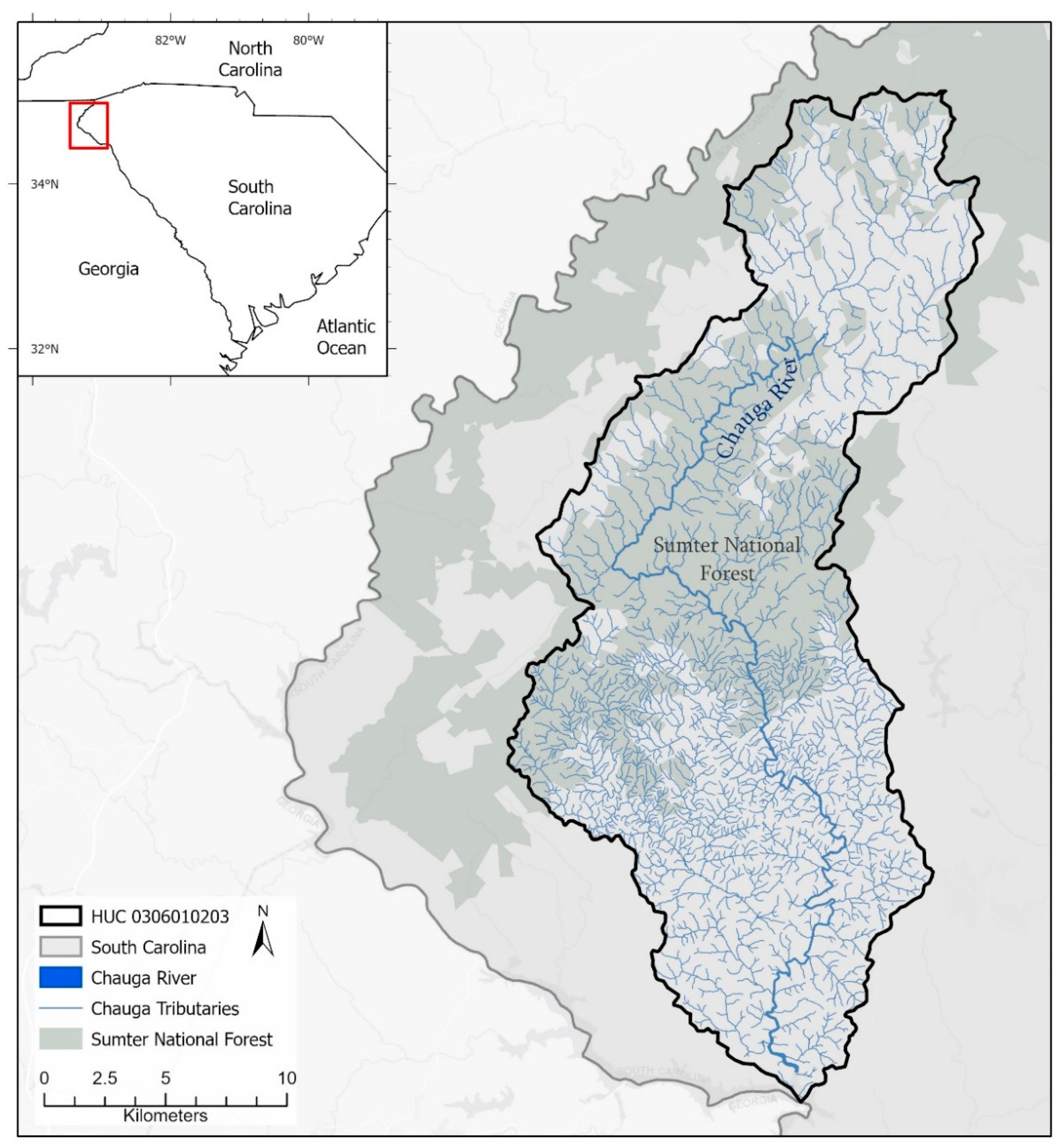
2.1. Study Area

The Chauga River watershed (10-digit HUC code: 0306010203) is located in Oconee County, SC, and is approximately 286 km2 (Figure 1). The Chauga River is close to 50 km in length, beginning south of Mountain Rest and flowing into the Tugaloo River and eventually the Savannah River at Lake Hartwell [33]. Approximately 28 km of the upper section of the river are inside the protected area of the Sumter National Forest (SNF), with the lower reaches of the river flowing through unprotected land. The watershed varies from steep mountainous terrain in the northwest to low rolling hills in the southeast and has an average gradient of 8.7 m per km [34]. The river is classified as a freestone river at the upper reaches and is characterized by steep gradients and fast currents for about 16 km [34,35,36]. The most common soils for the area are acidic colluvial soils often found on steep slopes (50–80%) [33].

2.2. Stream Data

A stream width polygon for the Chauga River was obtained from SC Department of Natural Resources (SCDNR) (Table 2) and buffered by 50 m to capture the adjacent riparian area. The single line stream data representing the tributaries were combined with the stream connector polylines and the stream centerline data where the streamlines were disconnected to create a continuous streamline for the tributaries of the Chauga River. The resulting tributary streamlines were buffered by 50 m because previous studies have found this buffer width captures shading of the river [1]. The overlapping area of the tributary buffer and the Chauga River buffer was removed from the tributary buffer so that the area would not be captured twice.

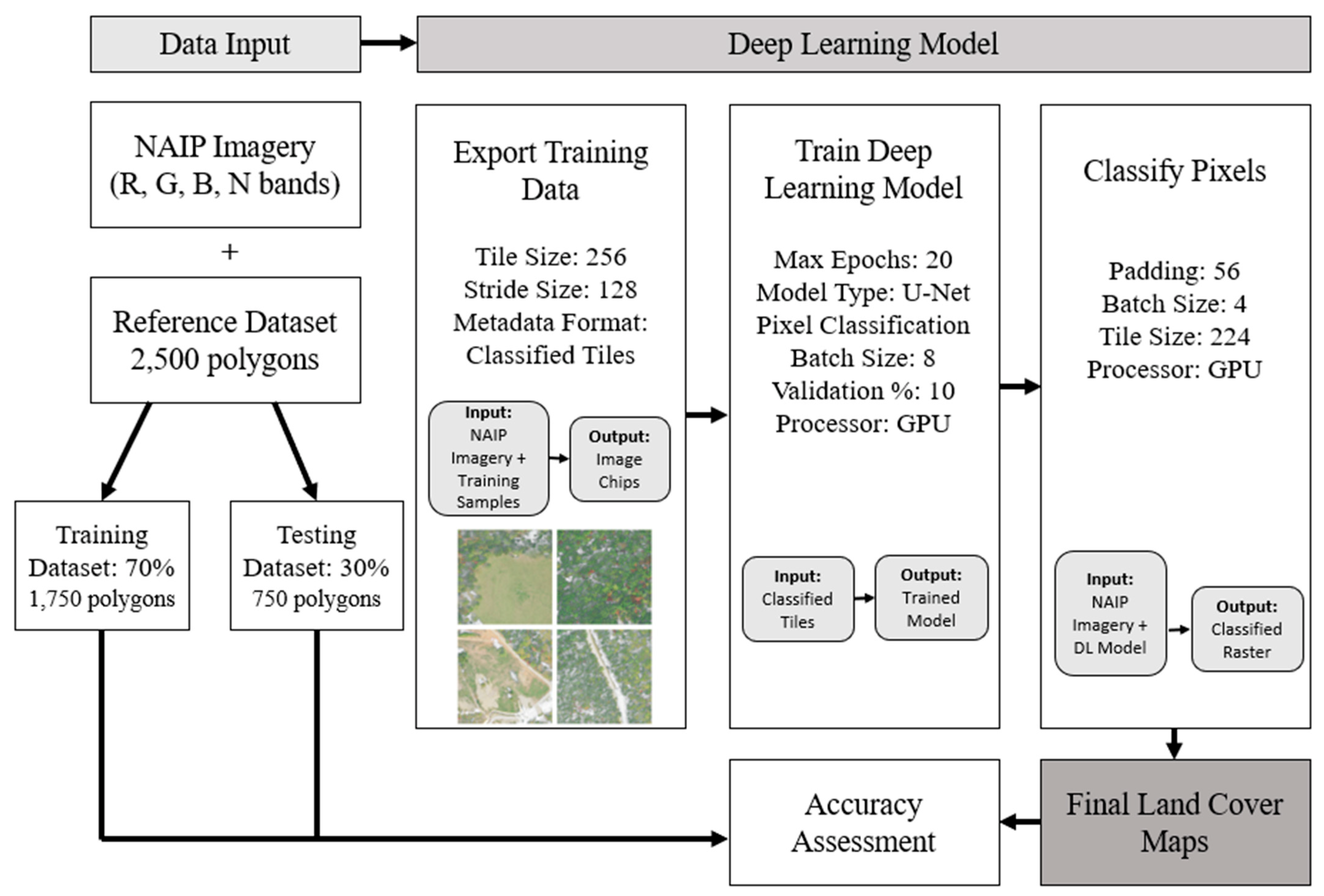
2.3. Image Classification

Figure 2 illustrates the workflow of the imagery classification. First, 2011 and 2019 imagery were obtained from the National Agriculture Imagery Program (NAIP) through the United States Geological Survey (USGS) EarthExplorer website. NAIP aerial imagery is taken during agricultural growing seasons to capture “leaf-on” conditions. The NAIP imagery contained four bands (red, green, blue, and near-infrared) and had a pixel size of 1 m for 2011 and a pixel size of 0.6 m for 2019 [37]. The study area consisted of 18 image tiles from April 2011 and 18 image tiles from September and October 2019. Each image tile for both years was 3.75 × 3.75-min quarter quadrangle plus a 300 meter buffer on all four sides. The 18 images for each year were mosaicked together to create a 2011 image and a 2019 image covering the study area using the NAD1983 UTM Zone 17M projection.
Next, the desired land cover classes in the final land cover maps were defined using recent classification work from Haq et al. (2021) [13] as a reference. A classification was created containing nine land cover classes: water, deciduous trees, evergreen trees, open land, riverbed, developed, roads, shadow (tree), and shadow (riverbed) (Table 3) [13].
A total of 2500 polygon samples were created to represent these land cover classes throughout the study area for the 2011 imagery, and a separate set of 2500 polygon samples were created for the 2019 imagery. The area of these polygon samples varied from 1 to 43,000 m2 to capture areas that were distinctly representative of the assigned land cover class without including parts of other land cover types. For instance, a training polygon would only contain pixels for one land cover class, such as water. Many sample polygons were very small to capture the fine level of detail over the landscape, such as shaded areas over the river or small areas of exposed riverbed. The very large training polygons often represented large areas of water or open land that had no land cover variation. The distribution of training samples by land cover class for 2011 and 2019 are seen in Table 3. The total number of samples for both years were split into training and testing data with a 0.7/0.3 split, creating 1750 training samples and 750 test samples for 2011 and a separate set of 1750 training samples and 750 test samples for 2019.
The NAIP imagery and land cover training polygons were then used to train a Deep Learning pixel classification model using a Deep Learning algorithm in ArcGIS Pro [38]. These deep learning models used the trained polygon samples to identify patterns in the spectral signature of the image’s pixels to then assign each pixel to the corresponding land cover classes.
The 2011 NAIP imagery and the 2011 training polygon land cover samples were exported as 256 × 256-pixel image chips (see examples of these image chips in Figure 2) to begin the deep learning model process. Each image chip had a 50% overlap with the previous chip. This was determined by the stride size, which was set to half the size of the tile. These image chips containing the training data were exported into a folder as classified tiles and used to train the deep learning model [39]. The same process was repeated for the 2019 NAIP imagery and corresponding training polygons.
A U-Net deep learning model was used because it has been shown to effectively classify pixels [40,41]. The max epochs were set to 20, meaning the training data were passed through the neural network a maximum of 20 times to reduce the error rate. However, the model was set to stop training when the model was no longer improving, despite the max epoch number. The batch size was set to 8, meaning the model processed eight training samples at a time. The validation percentage was set to 10, so 10% of the training samples were used to validate the deep learning model. A certain learning rate was not specified, but rather the best learning rate was determined by the model during the training process. The GPU processor was used.
Finally, the trained deep learning models were used to classify the 2011 and 2019 NAIP imagery into two separate land cover maps. These final land cover maps had the same resolution as the NAIP imagery (1 m for 2011 and 0.6 m for 2019). The model assigned each individual pixel to the corresponding land cover class it most closely matched as determined by the trained model, thereby producing high-resolution land cover maps. An accuracy assessment for each classification was calculated to understand the performance of the deep learning models. Overall accuracy, Kappa coefficient, consumer’s accuracy, and producer’s accuracy were calculated as part of the accuracy assessment.
Overall accuracy illustrates a total accuracy measurement for land cover classification by dividing the total number of correct pixel predictions by the total number of pixels. The Kappa coefficient is another common measurement of land cover classification accuracy and illustrates the difference between the classified image from the model’s predictions and the true land cover in reality [42]. Higher values for both statistics indicate that the land cover maps represent a more accurate classification of the image [42]. Consumer’s accuracy divides the number of correctly classified pixels in a particular land cover class with the total number of pixels in that land cover class [43]. Producer’s accuracy divides the number of correctly classified pixels for a land cover class by the total number of reference pixels for that land cover class [43].
The land cover in 2011 and 2019 was extracted for the 50 m buffers along the Chauga River and its tributaries to examine if there were any differences over the eight-year period. The land cover within these buffers was further divided into areas that fell inside and outside the Sumter National Forest to examine the land cover differences.

2.4. LiDAR Classification

LiDAR data were downloaded for Oconee County from SCDNR for 2011. To cover the study area, 44 .las files were downloaded, and all files were combined into a single dataset for the extent of the watershed. A digital surface model (DSM) was created by selecting first return LAS points. These first return points represent the first object hit by the LiDAR laser pulse, or the tallest feature in the landscape, such as the tops of vegetation and buildings [44]. The height measurements for these first return points were then rasterized into a DSM surface with 10 m resolution to represent the elevation of the study area, including the tops of vegetation and buildings.

2.5. Solar Radiation

Global solar radiation for the Chauga River was calculated with the Area Solar Radiation tool in ArcGIS Pro, which sums direct and diffuse radiation together [38]. This tool uses a hemispherical viewshed algorithm to calculate the amount of sun rays, or insolation, reaching a particular area and creates a surface raster of this information [45,46]. The Chauga stream polygon from SCDNR was buffered by 50 m to capture most of the shading in the riparian zone. The DSM described above was used as the input to calculate global solar radiation within the Chauga River riparian area. Using the DSM rather than the DEM in this calculation captured the influence vegetation has on solar radiation. Solar radiation was not calculated for the tributaries because there was very little exposed open water and most of the tributaries were completely covered in vegetation. The ‘Start day’ was set to 171 (20 June) and ‘End day’ to 265 (22 September) to capture the hottest summer months when insolation is greatest. The default settings were retained for all other fields (‘Sky size/Resolution’ = 200, ‘Time configuration’ = Multiple days, ‘Day interval’ = 14, ‘Hour interval’ = 0.5).

3. Results

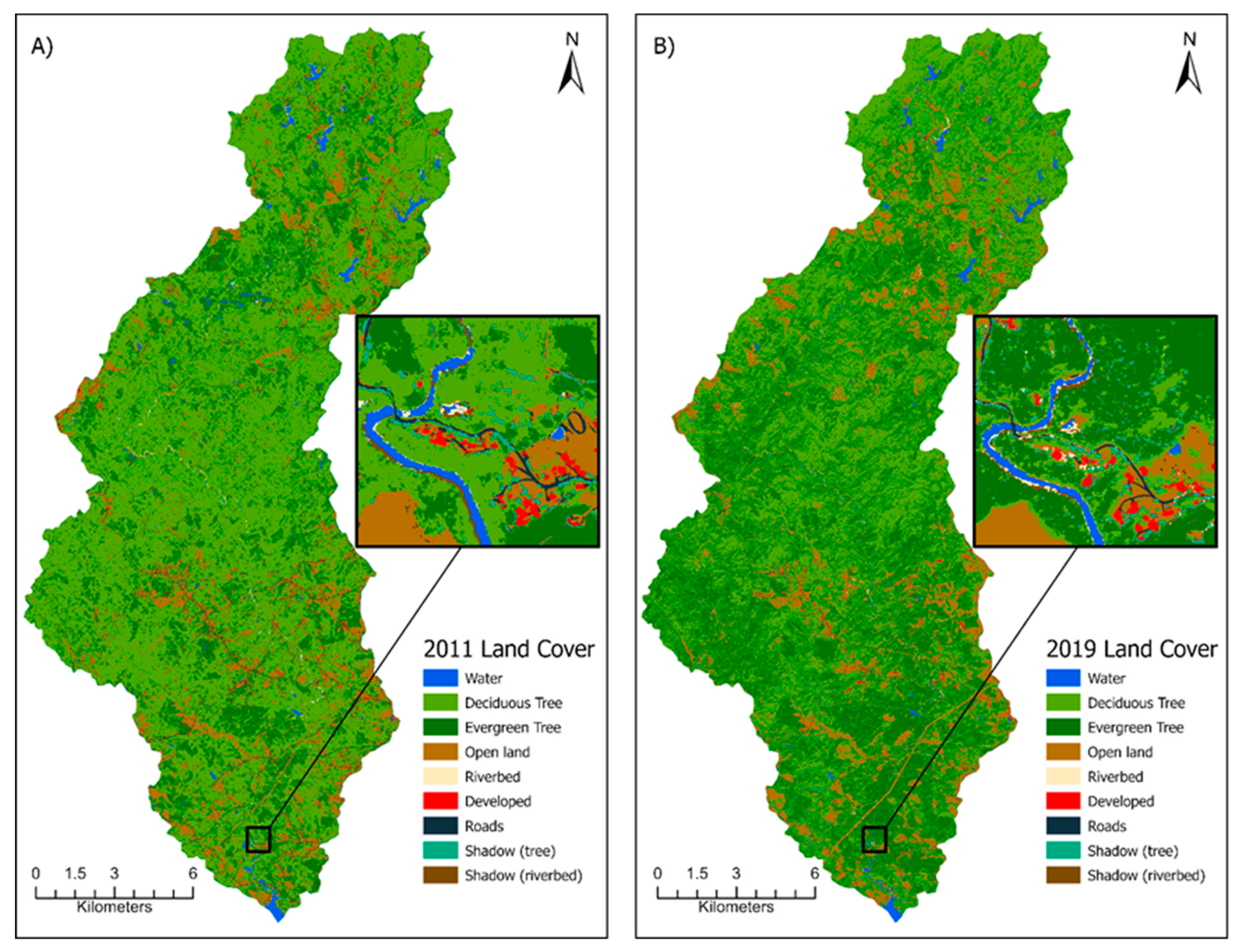
3.1. Land Cover and Shading Distribution in the Chauga River Watershed Using Deep Learning Classification of High-Resolution Imagery

The land cover classifications for 2011 and 2019, shown in Figure 3 were produced using deep learning models specific for each year. The 2011 deep learning classification produced higher overall accuracy than 2019, with overall accuracy assessments of 94.43% (2011), and 85.70% (2019), and the Kappa accuracies were 0.92 (2011) and 0.81 (2019). When the deciduous tree and evergreen tree land cover classes were combined into a single tree cover class, the overall accuracies increased to 96.7% (2011) and 95.3% (2019), with Kappa accuracies of 0.951 (2011) and 0.935 (2019) (Table 4). The 2019 classification was likely less accurate in separating deciduous and evergreen trees because the NAIP source imagery came from fall, when there is a less distinguishable difference between the two tree types, while the source imagery from 2011 came from spring.
Further examination of the accuracy assessment for the 2011 and 2019 deep learning classifications indicates that the deep learning models had high accuracy overall. This is because the overall accuracy exceeds the minimum 85% threshold for acceptance of land cover maps as set by Anderson [47], although a few land cover classes were not as accurate as evidenced by lower consumer’s and producer’s accuracy (Table 4). For instance, the riverbed land cover class had the lowest consumer’s error and a lower producer’s accuracy compared to other classes. Riverbed was difficult for the model to capture because training samples for the class included exposed rocks in the middle of the Chauga River and both sandy and muddy banks along the river. Visual inspection of the final land cover maps revealed that areas of sandy ground not identified as riverbed was sometimes classified as riverbed rather than open land. This was a more common problem with the 2019 model, as seen in the lower producer’s accuracy for riverbeds. Shadow cast by trees was also low in consumer’s accuracy because training samples for shadow amongst the trees may have included parts of tree pixels because the shade was so interspersed with tree vegetation in the imagery. Predictions for shadows cast over rivers were less accurate from the 2011 model. When excluding the riverbed and shadows cast by trees’ land cover classes, the accuracy of the 2011 and 2019 models are within a satisfactory range for accepting the final land cover maps.
There was little difference between 2011 and 2019 land cover when looking at the entire Chauga River watershed (Table 5). Land cover classes for water, open land, riverbed, developed, and shadow (riverbed) were all within a 1% difference from 2011 to 2019. The greatest difference in the two classifications was between the separation of deciduous and evergreen trees (2011: 66.10% deciduous, 17.68% evergreen) vs (2019: 49.04% deciduous, 33.61% evergreen). However, when the two tree cover classes were combined into a single tree cover class, there was little difference (2011: 83.78%, 2019: 82.65%). There was a 1.04% decrease in roads and a 2.41% area increase in shadows from trees in 2019.

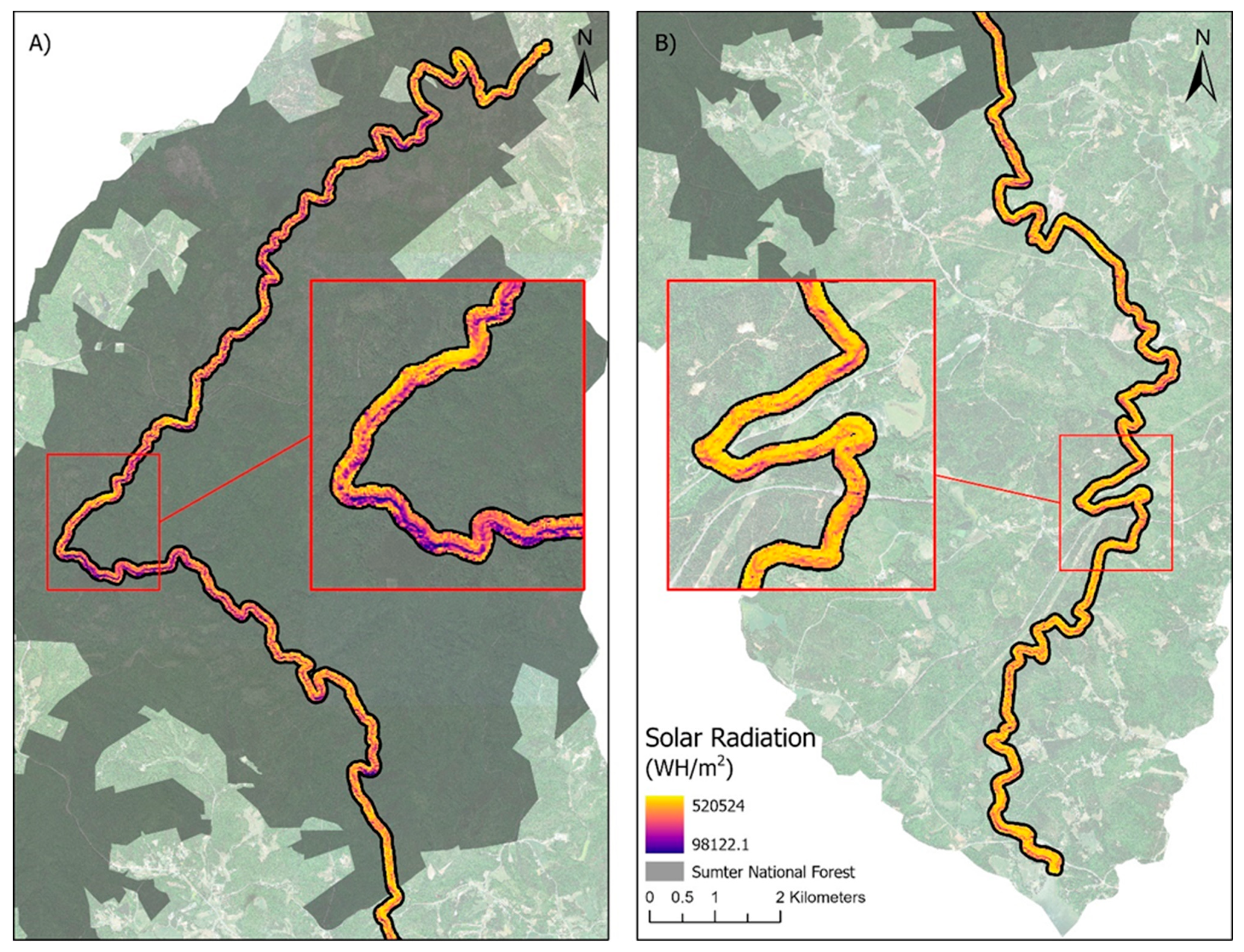
3.2. Incorporation of Vegetation Structure Using LiDAR to Calcualte Solar Radiation

Table 6 shows the solar radiation values calculated for the main stem of the Chauga River for the areas inside and outside SNF. The overall mean solar radiation values were higher in the area outside SNF (inside: 416, 770 WH/m2; outside: 455,845 WH/m2). The minimum and maximum solar radiation values are also higher outside SNF (min: 180,776 WH/m2; max: 520,230 WH/m2) compared to the values inside the protected area (min: 98,122 WH/m2; max: 520,093 WH/m2). The range of solar radiation values were greater inside SNF, indicating more temperature variability in this area (inside: 421,970 WH/m2; outside: 339,453 WH/m2). Figure 4 further illustrates this pattern of lower solar radiation values inside SNF.

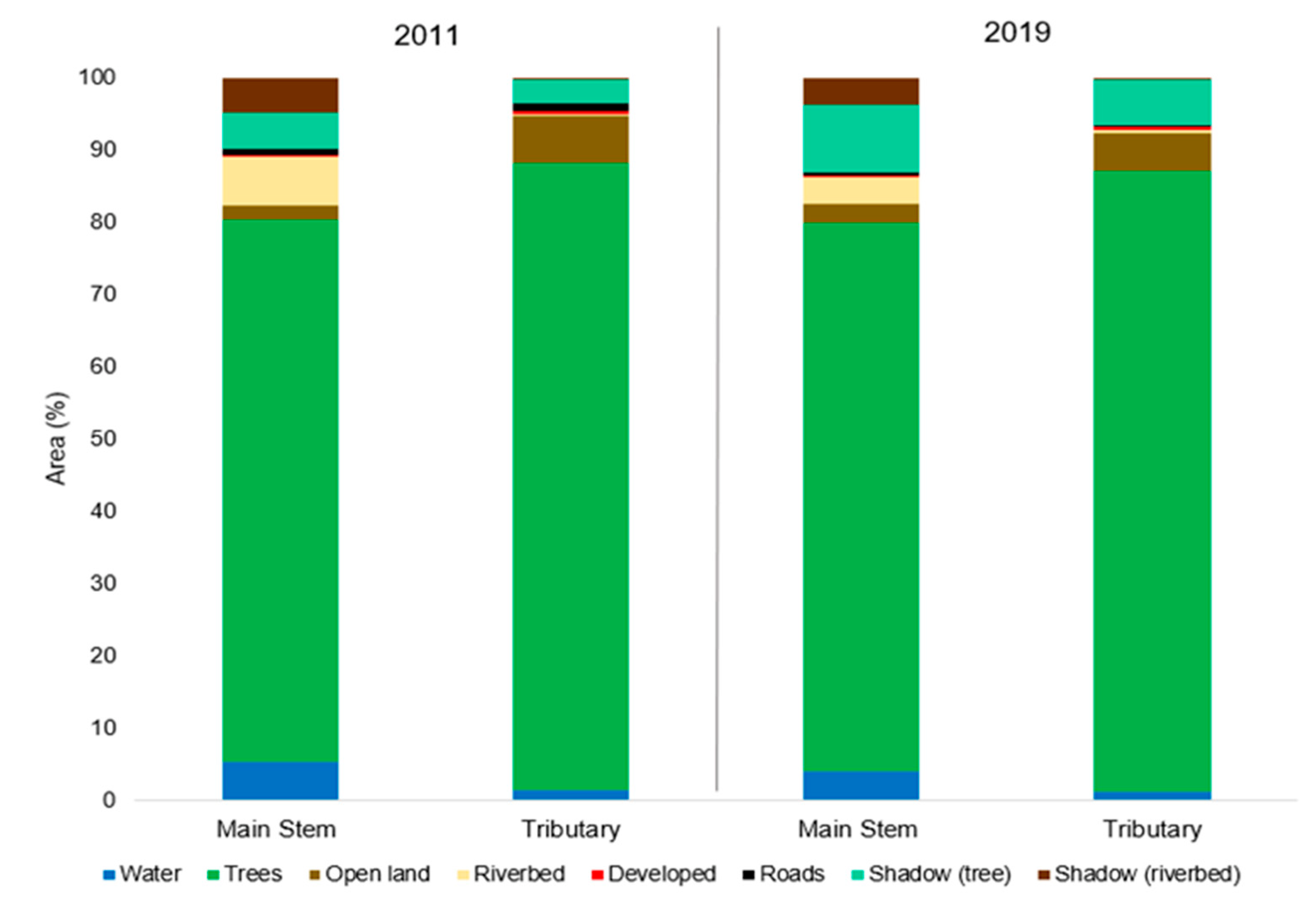
3.3. Land Cover and Shading along the Chauga River Main Stem and Chauga River Tributaries

Changes in land cover from 2011 to 2019 were more visible when the land cover was analyzed for the 50 m buffer around the main stem of the Chauga River and for the 50 m buffer around its tributaries (Figure 5, Table 7 and Table 8). In the Chauga River buffer, there was a 1.35% decrease in water area. Open land, developed area, and total tree cover increased by less than 1% from 2011 to 2019. There was a 3.04% decrease in riverbed, a 0.49% decrease in roads, a 1.05% decrease of shadows over riverbed, and 4.37% increase in shadows amongst tree canopy from 2011 to 2019. In the tributary buffer, there were less than 1% decreases in water, developed area, roads, and overall tree coverage. There were also less than 1% increases in riverbed and shadow over riverbed during the time period. Shadow in tree canopy area increased by 2.96%, and there was a 1.27% decrease in developed area.
Examination of the land cover within a 50 m buffer of the Chauga River main stem and within a 50 m buffer of the tributaries both inside and outside SNF for 2019 revealed differences in some land cover classes (Figure 6), with the biggest being less total tree coverage in the tributary buffer outside SNF vs. inside SNF (10.8%). There was also more open land in the tributary buffer outside SNF when compared to open land in the Chauga River buffer (6.68%). In addition, there was more open land in the tributary buffers outside SNF compared to inside the Chauga River buffers outside SNF (5.01%).
Developed area percentages were higher outside SNF compared to inside SNF when looking at both the Chauga River (0.36%, 0.1%) and tributary (0.49%, 0.11%) buffers. Similarly, road area was greater outside than inside SNF for the Chauga River buffer (0.3%, 0.12%) and the tributary buffer (0.6%, 0.09%), with a greater increase in roads seen in the tributaries. The water area was greater in the Chauga River buffer compared to the tributary buffer, both inside and outside SNF, because the Chauga River is wider than its tributaries, which are mostly covered by trees canopies. There was also more overall tree coverage in the tributary buffer than the Chauga River buffer because the Chauga River is wider.

4. Discussion

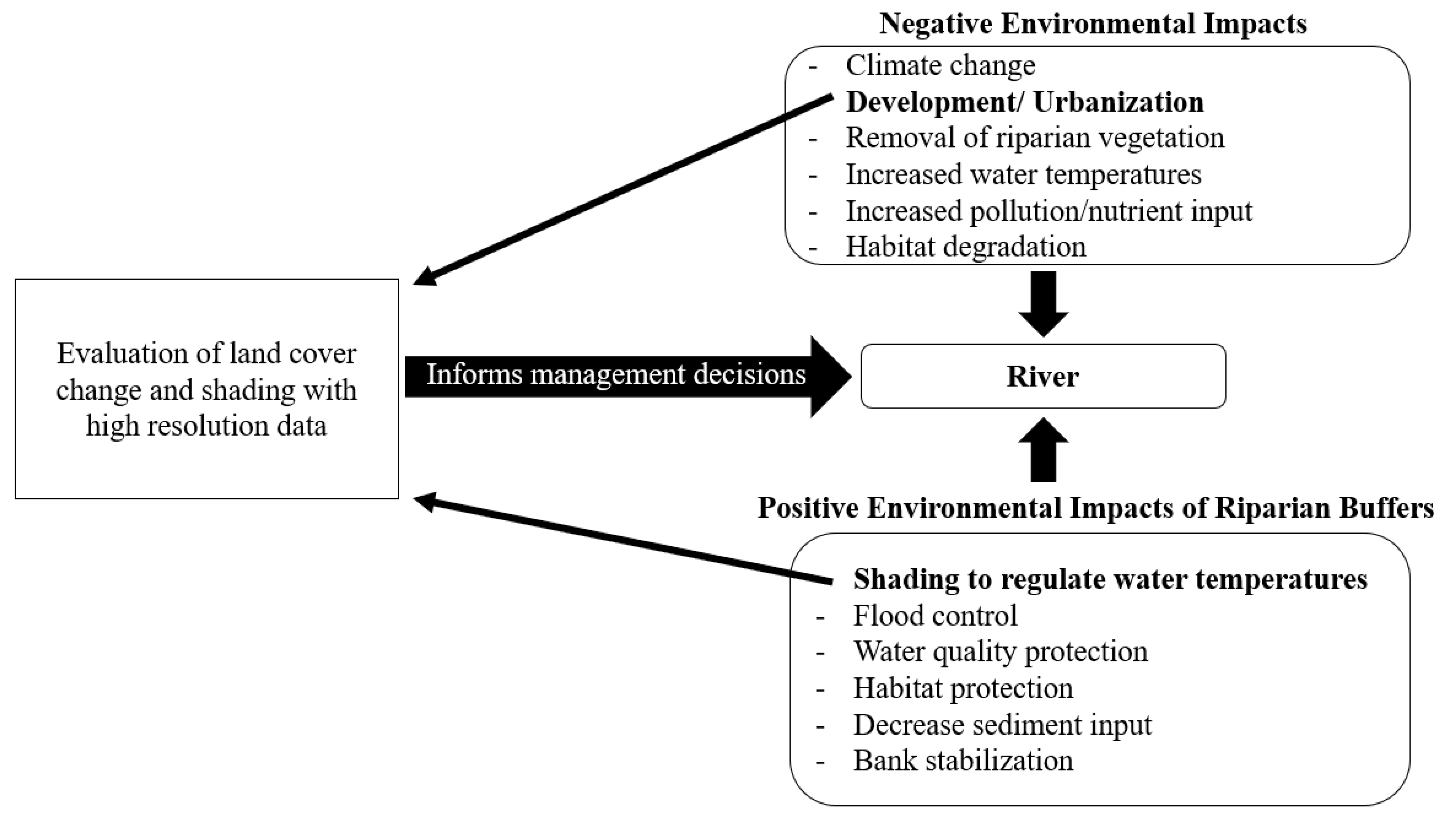
4.1. Importance of Monitoring Riparian Buffers

Riparian buffers are critical to monitor with changing climate in riverine systems because of the numerous ways these systems can be impacted and the buffer’s protective function. Development and urbanization of the areas along rivers can degrade river ecosystems [48]. The resulting changes of land cover in riparian buffers can lead to increased water temperatures if vegetation cover is removed and a decrease in water quality as vegetation is no longer present to trap pollutants before they enter waterways [5,8]. Additionally, human disturbance of riparian buffers and removal of native vegetation can introduce invasive species that can degrade buffer biodiversity and function, altering natural river ecosystem functions [49]. All of these impacts could affect rivers, leading to degraded water quality, impaired habitat for aquatic species, and overall, less resilient ecosystems.
Vegetated riparian buffers around rivers protect river systems in various ways (Figure 7). For instance, riparian buffers protect water quality by preventing excess nutrients such as nitrate, nitrogen, and phosphorus from running off of neighboring croplands or open areas into rivers [50,51,52]. If excess nutrients are not removed but rather enter rivers, this could lead to eutrophication, excess plant growth, and fish kill as a result of depleted oxygen [50]. Riparian buffers can decrease erosion of riverbanks and provide stability [53,54]. With improved bank stability, riparian buffers can also reduce sediment flow into rivers during rain events, thereby preventing spikes in turbidity that can harm aquatic life [52,55,56]. In addition, riparian buffers help preserve fish by maintaining food availability and decreasing the number of times water temperatures are greater than what can be tolerated by fish populations such as smallmouth bass and trout [57,58,59]. Riparian buffers can protect against the increased storm surge flooding that will occur with climate change, by reducing the velocity of flowing water and by storing water [5,49]. Overall, riparian buffers can be important management tools for bolstering river systems against climate change.

4.2. Use of High-Resolution Imagery and LiDAR Data to Evaluate Shading

Deep learning land cover classification produced an overall accuracy of 95.3% for 2011 and 96.7% for 2019 when tree cover was generalized. Similar to a recent study [13], this high accuracy deep learning method for land cover classification enabled the distinction between shadows cast over the river from shadows cast by trees in forests or over open land, as well as a detailed and accurate record of riparian tree cover. Given the small pixel size of the imagery and the high overall accuracies and Kappa coefficients of the final land cover maps, these land cover maps can be accepted as an accurate representation of the land cover of the study area. The land cover classes of most importance to this study were water, trees, open land, development, roads, and shadows over rivers. These land cover classes had high consumer’s and producer’s accuracies of over 70%, so this methodology of deep learning models to classify high resolution remotely sensed images is one that can be applied to other watersheds to establish current baseline conditions and monitor change over time. With continually improving remote sensing imagery and advancements in deep learning techniques, higher accuracy land cover classifications at higher spatial resolutions such as this one can be achieved.
Similar advancements in LiDAR technology are making data more widely available for landscape-scale analysis. Like in similar research [60,61], this study was able to incorporate riparian vegetation into the calculation of solar radiation on the Chauga River, through the use of LiDAR. When the solar radiation values were mapped, areas of lower solar radiation aligned with the shaded river land cover class, illustrating the importance of riparian shade over river channels to protect against increasing temperatures from climate change.
It is important to note that while these remote sensing techniques for land cover classification are effective and efficient methods for understanding a landscape for management needs, there are limitations that impact the interpretability of the results. The deep learning models were trained by drawing sample polygons throughout the landscape, and therefore, contain a level of training bias. The models also depend on the aerial imagery used, which in this case were taken at a single snapshot in time. The difference in deciduous and evergreen tree differentiation by the 2011 and 2019 models was evidenced by the seasonal difference of the aerial imagery used [62,63]. The aerial imagery in 2011 was taken in April, while the imagery in 2019 was taken in September and October. This seasonal difference impacts the spectral signature of the images, as the new leaf growth in deciduous trees was more distinct from evergreen vegetation in spring compared with the fall. Therefore, the two tree types were combined into one tree land cover class to produce more accurate final land cover maps. The seasonal difference between the 2011 and 2019 images also contributed to the difference in the water land cover class. Less water in 2019 was likely due to increased evapotranspiration during the summer months, leading to drier river stretches. This was evidenced in the aerial imagery as several areas covered in water in spring of 2011 were dry sandbars or mud flats in early fall of 2019. Additionally, the time of day when the NAIP aerial imagery was collected also impacts the amount of shade identified in the landscape because of the orientation of the sun. The difference in time of day flown could have contributed to the slight differences in the shade over the riverbed and in the trees between 2011 and 2019. Ideally, future studies that use deep learning to examine land cover changes with NAIP imagery should select years that have images flown at the same time of year to combat the seasonal impact on training the models. Finally, despite using very high-resolution NAIP imagery with small pixel sizes (2011: 1 m; 2019: 0.6 m), it was more difficult for the models to differentiate land cover classes for the pixels between two different land cover classes. For instance, in areas between road and open land, the models could misclassify these in-between pixels to the wrong land cover class.
While the changes in land cover classes were not very different over this 8-year period for the Chauga River watershed, the examination of land cover at such a high resolution enables these differences to still be detectable. Without the use of the NAIP imagery and the deep learning models, these differences in land cover changes may not have been noticed. Early detection of these gradual changes can help land managers and local agencies plan to ensure sustainable growth that does not negatively impact the riparian buffers of the Chauga River and its tributaries.

4.3. Land Cover and Shading Influence on River Temperature

When examining the land cover results from 2011 and 2019 for the main stem Chauga River and its tributaries, there were no major changes over the course of the eight years. This could be because they occur in a more rural area of the county, and the increase in population has not led to greatly increased development yet. Similarly, the land cover was examined within the 50 m riparian buffers of the Chauga main stem and its tributaries, so development pressures may not yet be strong enough to encroach on these riparian zones. Therefore, the more obvious differences in land cover were seen in the differences in protected vs. unprotected areas, which illustrated our expected result that there would be more development, roads, and open land outside of SNF.
While the results of this study did not illustrate an increase in development pressure to the Chauga River, they illustrate an appropriate methodology that can be applied to other watersheds. Furthermore, the land cover maps provide baseline data for the Chauga watershed that can equip land managers and local agencies to make decisions about protecting the overlooked tributaries of the Chauga River. That way, if development does accelerate in the unprotected areas outside of SNF along the tributaries, the riparian canopy cover will decrease, allowing direct solar radiation to increase the water temperatures. Water temperatures of the tributaries play a contributing role in the overall main stem temperature [2], with any increased temperatures of the tributaries flowing into and impacting the main stem of the Chauga River. Although the Chauga River’s banks are protected from major disturbance through designation as a Scenic Area under the Wild and Scenic River Act [23], development in its unprotected tributaries can negatively impact the overall quality of the Chauga River.
Recent research on the impact of riparian vegetation on water temperature [64] found that even sparse vegetation can protect water temperatures from spiking. Another study on land cover types on water temperature showed that tree cover is negatively correlated with water temperature, and development has a positive correlation with water temperature [65]. These results give further interpretability to what was found in the Chauga River watershed as there were higher solar radiation values outside the protected area, where there was less tree cover and greater development. While riparian shading does help prevent water temperature increases, studies have also found shading to limit aquatic plant biodiversity [66], so management strategies should also consider the shading needs of the aquatic vegetation rivers before planting vegetation in riparian zones to prevent water temperature increases.

4.4. Protected Area Impact on Land Cover Change in the Chauga River Watershed

Protected area has limited development and decreased tree cover loss along the Chauga River. In 2011, there was 1.25% more open land in the Chauga River riparian area outside of the SNF, and in 2019, there was 1.81% more open land outside the SNF. This difference in greater open land outside SNF is even more evident when examining the riparian area of the tributaries. In 2011, there was 8.55% more open land outside the protected area, and in 2019, there was 6.68% more. The preservation of tree cover due to the SNF is also evident when examining the difference in tree cover for the tributary riparian areas. There was 13.55% less tree cover along the tributaries outside SNF in 2011, and the area difference for 2019 was 10.81%. The effect of these land cover changes is then demonstrated by the greater solar radiation values for the Chauga River outside the protected area. This pattern will be exacerbated if development is left unchecked in this area.
With low levels of governmental protection for the tributaries of the Chauga River, these riparian areas are critical to monitor. Despite the lack of protection, these tributaries are important aspects of the river system because they flow into the main stem, carrying sediment, pollutants, organic matter, and potentially different water temperatures [67]. If these elements greatly differ from conditions in the main stem of the river, then the flow from tributaries could degrade the quality of the main river. This study illustrates the difference in land cover change around the tributaries compared to the main stem of the Chauga River. With more open land and development in the tributary buffers, this could lead to more nutrient and pollutant runoff into the tributaries themselves, which would then flow into the main stem of the Chauga River. Thus, it is critical to monitor and protect the riparian buffers around a river’s tributaries.

5. Conclusions

This study illustrates the importance of high-resolution data to monitor these riparian areas by using remotely sensed imagery with 0.6–1 m resolution and LiDAR data with a point density of 1 point per square meter. Until recently, satellite images with low resolutions, such as 30 m, were used to examine landscapes. At this coarse scale, details such as shading over a narrow river such as the Chauga were impossible to distinguish, and accurate information could not be derived for very small tributaries. A recent study that compared land cover classifications and water quality modeling results for 1 m and 30 m resolution images found the higher resolution imagery produced more accurate results [68]. In previous studies using 30 m pixels, the land cover maps are not as accurate because the pixels are so large that they contain multiple land cover classes, but the model must only assign one land cover class to that pixel, leading to over and under-representation of the area’s land cover. However, with the use of 0.6 m and 1 m pixels, each pixel typically represents only one land cover class. Therefore, the advancements in available data at high resolutions have made a detailed investigation of riparian areas and river shading in both protected and developing areas, possible with remarkable accuracy.
This study demonstrates a successful framework of deep learning land classification and solar radiation calculations to evaluate the shading of the Chauga river system over time that, when combined, can be used to monitor the influences on water temperature and can inform management strategies needed to prevent increased temperatures in the rivers. This methodology can be applied to other systems to understand the protection and shading of rivers, along with changes over time, and can determine management needs, such as riparian plantings, necessary to ensure long-term protection of rivers as the climate continues to change. In addition, deep learning land cover classification can be used to carefully monitoring changes in tree cover caused by development or natural causes such as disease. Likewise, LiDAR-based tree shading modeling can provide a detailed evaluation of shading of these important water resources. Such studies about river systems provide important baseline information for local governments and protected area managers to collectively balance increased development with the continued preservation of natural resources as the climate continues to change.

Author Contributions

Conceptualization C.J.P.; methodology and software, M.M.B., C.J.P. and H.A.Z.; data curation, writing—original draft preparation, and visualization, M.M.B., A.P.G., E.A.S. and H.A.Z.; writing—review and editing, C.J.P., E.A.M., A.P.G., E.A.S. and H.A.Z.; supervision, and project administration, C.J.P. All authors have read and agreed to the published version of the manuscript.

Funding

The publishing of this article was partially supported by the Clemson University Libraries Open Access Publishing Fund and the Clemson Department of Forestry and Environmental Conservation.

Data Availability Statement

Data are not available for sharing.

Acknowledgments

We would like to thank the reviewers for their constructive feedback. We would also like to thank the graduate students in FOR 8160: Remote Sensing & GIS (Spring 2021) for gathering the data for this project.

Conflicts of Interest

The authors declare no conflict of interest.

References

  1. Bachiller-Jareno, N.; Hutchins, M.G.; Bowes, M.J.; Charlton, M.B.; Orr, H.G. A novel application of remote sensing for modelling impacts of tree shading on water quality. J. Environ. Manag. 2019, 230, 33–42. [Google Scholar] [CrossRef] [PubMed]
  2. Johnson, M.F.; Wilby, R.L. Seeing the landscape for the trees: Metrics to guide riparian shade management in river catchments. Water Resour. Res. 2015, 51, 3754–3769. [Google Scholar] [CrossRef] [Green Version]
  3. Martin-Ortega, J.; Ferrier, R.C.; Gordon, I.J.; Khan, S. Water Ecosystem Services: A Global Perspective; UNESCO Publishing: Paris, France, 2015; pp. 19–21. [Google Scholar]
  4. van Vliet, M.T.H.; Franssen, W.H.P.; Yearsley, J.R.; Ludwig, F.; Haddeland, I.; Lettenmaier, D.P.; Kabat, P. Global river discharge and water temperature under climate change. Glob. Environ. Chang. 2013, 23, 450–464. [Google Scholar] [CrossRef]
  5. Palmer, M.A.; Lettenmaier, D.P.; Poff, N.L.; Postel, S.L.; Richter, B.; Warner, R. Climate change and river ecosystems: Protection and adaptation options. Environ. Manag. 2009, 44, 1053–1068. [Google Scholar] [CrossRef] [PubMed]
  6. Ghermandi, A.; Vandenberghe, V.; Benedetti, L.; Bauwens, W.; Vanrolleghem, P.A. Model-based assessment of shading effect by riparian vegetation on river water quality. Ecol. Eng. 2009, 35, 92–104. [Google Scholar] [CrossRef]
  7. Johnson, R.K.; Almlöf, K. Adapting boreal streams to climate change: Effects of riparian vegetation on water temperature and biological assemblages. Freshw. Sci. 2016, 35, 984–997. [Google Scholar] [CrossRef]
  8. Dugdale, S.J.; Hannah, D.M.; Malcolm, I.A. An evaluation of different forest cover geospatial data for riparian shading and river temperature modelling. River Res. Appl. 2020, 36, 709–723. [Google Scholar] [CrossRef]
  9. Kussul, N.; Lavreniuk, M.; Skakun, S.; Shelestov, A. Deep learning classification of land cover and crop types using remote sensing data. IEEE Geosci. Remote Sens. 2017, 14, 778–782. [Google Scholar] [CrossRef]
  10. Kwan, C.; Ayhan, B.; Budavari, B.; Lu, Y.; Perez, D.; Li, J.; Bernabe, S.; Plaza, A. Deep learning for land cover classification using only a few bands. Remote Sens. 2020, 12, 2000. [Google Scholar] [CrossRef]
  11. Zhu, X.X.; Tuia, D.; Mou, L.; Xia, G.S.; Zhang, L.; Xu, F.; Fraundorfer, F. Deep learning in remote sensing: A comprehensive review and list of resources. IEEE Geosci. Remote Sens. 2017, 5, 8–36. [Google Scholar] [CrossRef] [Green Version]
  12. Helber, P.; Bischke, B.; Dengel, A.; Borth, D. EuroSAT: A novel dataset and deep learning benchmark for land use and land cover classification. IEEE J. Sel. Top. Appl. Earth Obs. Remote Sens. 2019, 12, 2217–2226. [Google Scholar] [CrossRef] [Green Version]
  13. Haq, M.A.; Rahaman, G.; Baral, P.; Ghosh, A. Deep learning based supervised image classification using UAV images for forest areas classification. J. Indian Soc. Remote Sens. 2021, 49, 601–606. [Google Scholar] [CrossRef]
  14. Hansen, M.C.; Loveland, T.R. A review of large area monitoring of land cover change using Landsat data. Remote Sens. Environ. 2012, 122, 66–74. [Google Scholar] [CrossRef]
  15. Gómez, C.; White, J.C.; Wulder, M.A. Optical remotely sensed time series data for land cover classification: A review. ISPRS J. Photogramm. Remote Sens. 2016, 116, 55–72. [Google Scholar] [CrossRef] [Green Version]
  16. Phiri, D.; Morgenroth, J. Developments in Landsat land cover classification methods: A review. Remote Sens. 2017, 9, 967. [Google Scholar] [CrossRef] [Green Version]
  17. Loicq, P.; Moatar, F.; Jullian, Y.; Dugdale, S.J.; Hannah, D.M. Improving representation of riparian vegetation shading in a regional stream temperature model using LiDAR data. Sci. Total Environ. 2018, 624, 480–490. [Google Scholar] [CrossRef]
  18. Seixas, G.B.; Beechie, T.J.; Fogel, C.; Kiffney, P.M. Historical and future stream temperature change predicted by a lidar-based assessment of riparian condition and channel width. J. Am. Water Resour. Assoc. 2018, 54, 974–991. [Google Scholar] [CrossRef]
  19. Olpenda, A.S.; Stereńczak, K.; Będkowski, K. Modeling solar radiation in the forest using remote sensing data: A review of approaches and opportunities. Remote Sens. 2018, 10, 694. [Google Scholar] [CrossRef] [Green Version]
  20. U.S. Census Bureau. County Population Totals: 2010–2019. Available online: https://www.census.gov/data/datasets/time-series/demo/popest/2010s-counties-total.html (accessed on 9 August 2021).
  21. Khatri, N.; Tyagi, S. Influences of natural and anthropogenic factors on surface and groundwater quality in rural and urban areas. Front. Life Sci. 2015, 8, 23–39. [Google Scholar] [CrossRef]
  22. Best, J. Anthropogenic stresses on the world’s big rivers. Nat. Geosci. 2019, 12, 7–21. [Google Scholar] [CrossRef]
  23. Robert, J. Revised Land and Resource Management Plan; Sumter National Forest: Clinton, SC, USA, 2004. [Google Scholar]
  24. What Are Wild and Scenic Rivers? (U.S. National Park Service). Available online: https://www.nps.gov/orgs/1912/what-are-wild-and-scenic-rivers.htm (accessed on 9 August 2021).
  25. Bartnik, A.; Moniewski, P. River bed shade and its importance in the process of studying of the fundamental physico-chemical characteristics of small river waters. In Contemporary Problems of Management and Environmental Protection. Issues of landscape Conservation and Water Management in Rural Areas; Faculty of Environmental Management and Agriculture, Olsztynwamia and University of Warmia and Mazury in Olsztyn: Olsztyn, Poland, 2011; Volume 7, pp. 137–149. [Google Scholar]
  26. Morgan, A.M.; Royer, T.V.; David, M.B.; Gentry, L.E. Relationships among nutrients, chlorophyll-a, and dissolved oxygen in agricultural streams in Illinois. J. Environ. Qual. 2006, 35, 1110–1117. [Google Scholar] [CrossRef] [Green Version]
  27. Huang, J.; Klemas, V. Using remote sensing of land cover change in coastal watersheds to predict downstream water quality. J. Coast. Res. 2012, 28, 930–944. [Google Scholar] [CrossRef]
  28. Mahmood, R.; Pielke, R.A.; Hubbard, K.G.; Niyogi, D.; Bonan, G.; Lawrence, P.; McNider, R.; McAlpine, C.; Etter, A.; Gameda, S.; et al. Impacts of land use/land cover change on climate and future research priorities. Bull. Am. Meteorol. 2010, 91, 37–46. [Google Scholar] [CrossRef]
  29. Cole, L.J.; Stockan, J.; Helliwell, R. Managing riparian buffer strips to optimise ecosystem services: A review. Agric. Ecosyst. Environ. 2020, 296, 106891. [Google Scholar] [CrossRef]
  30. Edwards, I.F.; Drinkard, M.K. An unprotected tributary has no detectable impact on macroinvertebrates in a wild and scenic river in the Southeast (Chattooga). Bios 2021, 91, 167–172. [Google Scholar] [CrossRef]
  31. Dolloff, C.A. Monitoring for Changes in Chattooga River Mussel Populations. 2012–2019; Francis Marion-Sumter National Forest, South Carolina; USDA: Washington, DC, USA, 2020. [Google Scholar]
  32. Poling, B.T.; Dolloff, A.C. Soil Erosion from Eastern Hemlock (Tsuga Canadensis) Windthrow Mounds Following Hemlock Wooly Adelgid (Adelges Tsugae) Infestations in Riparian Areas If the Chattooga Wild and Scenic River and Tributaries; USDA: Washington, DC, USA, 2016. [Google Scholar]
  33. Creek, J. Chauga River 03060102-03. South Carolina Department of Health and Environmental Control; Savana River Basin: Georgia, SC, USA.
  34. Tobe, J.D.; Fairey, J.E., III; Gaddy, L.L. Vascular flora of the Chauga River Gorge Oconee County, South Carolina. Castanea 1992, 57, 77–109. [Google Scholar]
  35. O’Hara, K.; Becker, T.P. Tectonic assembly of the Brevard-Chauga Belt, South Carolina: Fluid inclusion evidence from Appalachian deep core site investigation hole 2 (ADCOH-2). J. Geodyn. 2004, 37, 565–581. [Google Scholar] [CrossRef]
  36. Acker, L.L.; Hatcher, R.D., Jr. Relationships between Structure and Topography in Northwest South Carolina, Geologic Notes; Division of Geology, State Development Board: Columbia, SC, USA, 1970; Volume 14, pp. 35–48. [Google Scholar]
  37. NAIP Imagery. Available online: https://fsa.usda.gov/programs-and-services/aerial-photography/imagery-programs/naip-imagery/index (accessed on 21 September 2021).
  38. ESRI. ArcGIS Pro: Release 7. Redlands, CA. 2021. Available online: https://www.esri.com/en-us/arcgis/products/arcgis-pro/overview (accessed on 17 September 2021).
  39. Classify Pixels Using Deep Learning (Image Analyst)—Arcgis Pro Documentation. Available online: https://pro.arcgis.com/en/pro-app/latest/tool-reference/image-analyst/classify-pixels-using-deep-learning.htm (accessed on 21 September 2021).
  40. Ronneberger, O.; Fischer, P.; Brox, T. U-Net: Convolutional Networks for Biomedical Image Segmentation. In Proceedings of the Medical Image Computing and Computer-Assisted Intervention-MICCAI 2015, Munich, Germany, 5–9 October 2015; Navab, N., Hornegger, J., Wells, W.M., Frangi, A.F., Eds.; Springer International Publishing: Cham, Germany, 2015; pp. 234–241. [Google Scholar]
  41. Zhang, Z.; Liu, Q.; Wang, Y. Road extraction by deep residual U-Net. IEEE Geosci. Remote 2018, 15, 749–753. [Google Scholar] [CrossRef] [Green Version]
  42. Monserud, R.A.; Leemans, R. Comparing global vegetation maps with the Kappa statistic. Ecol. Model. 1992, 62, 275–293. [Google Scholar] [CrossRef]
  43. Horning, N. Overview of Accuracy Assessment of Land Cover Products; American Museum of Natural History: New York, NY, USA, 2004; Volume 1, pp. 1–6. [Google Scholar]
  44. Dubayah, R.O.; Drake, J.B. Lidar remote sensing for forestry. J. For. 2000, 98, 44–46. [Google Scholar] [CrossRef]
  45. Rich, P.; Dubayah, R.; Hetrick, W.; Saving, S. Using viewshed models to calculate intercepted solar radiation: Applications in ecology. American Society for Photogrammetry and Remote Sensing Technical Papers. In Proceedings of the American Society of Photogrammetry and Remote Sensing; 1994; pp. 524–529. Available online: http://www.professorpaul.com/publications/rich_et_al_1994_asprs.pdf (accessed on 15 September 2021).
  46. Fu, P.; Rich, P.M. A geometric solar radiation model with applications in agriculture and forestry. Comput. Electron. Agric. 2002, 37, 25–35. [Google Scholar] [CrossRef]
  47. Anderson, J.R. A Land Use and Land Cover Classification System for Use with Remote Sensor Data; US Government Printing Office: Washington, DC, USA, 1976; Volume 964. [Google Scholar]
  48. May, C.W.; Horner, R.R. The cumulative impacts of watershed urbanization on stream-riparian ecosystems. In Proceedings of the American Water Resources Association International Conference on Riparian Ecology and Management in Multi-Land Use Watersheds, Portland, OR, USA, 28–31 August 2000; pp. 281–286. [Google Scholar]
  49. Johnson, L.R.; Trammell, T.L.E.; Bishop, T.J.; Barth, J.; Drzyzga, S.; Jantz, C. Squeezed from all sides: Urbanization, invasive species, and climate change threaten riparian forest buffers. Sustainability 2020, 12, 1448. [Google Scholar] [CrossRef] [Green Version]
  50. Jordan, T.E.; Correll, D.L.; Weller, D.E. Nutrient interception by a riparian forest receiving inputs from adjacent cropland. J. Environ. Qual. 1993, 22, 467–473. [Google Scholar] [CrossRef] [Green Version]
  51. Pinay, G.; Roques, L.; Fabre, A. Spatial and temporal patterns of denitrification in a riparian forest. J. Appl. Ecol. 1993, 30, 581–591. [Google Scholar] [CrossRef]
  52. Lee, K.-H.; Isenhart, T.M.; Schultz, R.C.; Mickelson, S.K. Multispecies riparian buffers trap sediment and nutrients during rainfall simulations. J. Environ. Qual. 2000, 29, 1200–1205. [Google Scholar] [CrossRef]
  53. Nakao, M.; Sohngen, B. The effect of site quality on the costs of reducing soil erosion with riparian buffers. J. Soil Water Conserv. 2000, 55, 231–237. [Google Scholar]
  54. Wynn, T.M.; Mostaghimi, S.; Alphin, E.F. The effects of vegetation on stream bank erosion. In Proceedings of the 2004 ASAE Annual Meeting, Ottawa, ON, Canada, 1–4 August 2004; Volume 1. [Google Scholar]
  55. Momm, H.G.; Bingner, R.L.; Yuan, Y.; Locke, M.A.; Wells, R.R. Spatial characterization of riparian buffer effects on sediment loads from watershed systems. J. Environ. Qual. 2014, 43, 1736–1753. [Google Scholar] [CrossRef]
  56. Zhang, C.; Li, S.; Qi, J.; Xing, Z.; Meng, F. Assessing impacts of riparian buffer zones on sediment and nutrient loadings into streams at watershed scale using an integrated REMM-SWAT model. Hydrol. Process. 2017, 31, 916–924. [Google Scholar] [CrossRef]
  57. Fischer, J.R.; Quist, M.C.; Wigen, S.L.; Schaefer, A.J.; Stewart, T.W.; Isenhart, T.M. Assemblage and population-level responses of stream fish to riparian buffers at multiple spatial scales. Trans. Am. Fish. Soc. 2010, 139, 185–200. [Google Scholar] [CrossRef]
  58. Albertson, L.K.; Ouellet, V.; Daniels, M.D. Impacts of stream riparian buffer land use on water temperature and food availability for fish. J. Freshw. Ecol. 2018, 33, 195–210. [Google Scholar] [CrossRef] [Green Version]
  59. Knouft, J.H.; Botero-Acosta, A.; Wu, C.-L.; Charry, B.; Chu, M.L.; Dell, A.I.; Hall, D.M.; Herrington, S.J. Forested riparian buffers as climate adaptation tools for management of riverine flow and thermal regimes: A case study in the Meramec River Basin. Sustainability 2021, 13, 1877. [Google Scholar] [CrossRef]
  60. Bode, C.A.; Limm, M.P.; Power, M.E.; Finlay, J.C. Subcanopy solar radiation model: Predicting solar radiation across a heavily vegetated landscape using LiDAR and GIS solar radiation models. Remote Sens. Environ. 2014, 154, 387–397. [Google Scholar] [CrossRef]
  61. Kaluża, T.; Sojka, M.; Wróżyński, R.; Jaskula, J.; Zaborowski, S.; Hämmerling, M. Modeling of river channel shading as a factor for changes in hydromorphological conditions of small lowland rivers. Water 2020, 12, 527. [Google Scholar] [CrossRef] [Green Version]
  62. Pankiw, J.; Piwowar, J. Seasonality of imagery: The impact on object-based classification accuracy of shelterbelts. Prairie Perspect. Geogr. Essays 2010, 13, 39–48. [Google Scholar]
  63. Grădinaru, S.R.; Kienast, F.; Psomas, A. Using multi-seasonal Landsat imagery for rapid identification of abandoned land in areas affected by urban sprawl. Ecol. Indic. 2019, 96, 79–86. [Google Scholar] [CrossRef]
  64. Kalny, G.; Laaha, G.; Melcher, A.; Trimmel, H.; Weihs, P.; Rauch, H.P. The influence of riparian vegetation shading on water temperature during low flow conditions in a medium sized river. Knowl. Manag. Aquat. Ecosyst. 2017, 5. [Google Scholar] [CrossRef] [Green Version]
  65. Horne, J.P.; Hubbart, J.A. A spatially distributed investigation of stream water temperature in a contemporary mixed-land-use watershed. Water 2020, 12, 1756. [Google Scholar] [CrossRef]
  66. Jusik, S.; Staniszewski, R. Shading of river channels as an important factor reducing macrophyte biodiversity. Pol. J. Environ. Stud. 2019, 28, 1215–1222. [Google Scholar] [CrossRef]
  67. Rice, S.; Roy, A.; Rhoads, B. River Confluences, Tributaries and The Fluvial Network; John Wiley & Sons: Hoboken, NJ, USA, 2008; pp. 209–217. ISBN 978-0-470-76037-6. [Google Scholar]
  68. Fisher, J.R.B.; Acosta, E.A.; Dennedy-Frank, P.J.; Kroeger, T.; Boucher, T.M. Impact of satellite imagery spatial resolution on land use classification accuracy and modeled water quality. Remote Sens. Ecol. Conserv. 2018, 4, 137–149. [Google Scholar] [CrossRef]
Figure 1. Location of the study area, the Chauga River watershed, in Oconee County, SC, USA.
Remotesensing 13 04172 g001
Figure 2. Workflow of the creation of the land cover maps using deep learning. This process was conducted twice, once with 2011 NAIP imagery and once with 2019 NAIP imagery.
Remotesensing 13 04172 g002
Figure 3. Land cover classification of the Chauga watershed: (A) 2011 and (B) 2019.
Remotesensing 13 04172 g003
Figure 4. Solar radiation values in the Chauga main stem inside the Sumter National Forest (A) and below the Sumter National Forest (B). WH/m2 is watt-hour per square meter.
Remotesensing 13 04172 g004
Figure 5. Land cover area (%) for 2011 and 2019 in the riparian areas of the Chauga main stem and tributaries. Deciduous and evergreen tree land cover classes were combined into a single tree class.
Remotesensing 13 04172 g005
Figure 6. Land cover area for 2019 for the main stem and tributary riparian areas inside and outside of Sumter National Forest. Deciduous and evergreen tree land cover classes were combined into a single tree class.
Remotesensing 13 04172 g006
Figure 7. Illustration of how the evaluation of shading and land cover in this study establishes a framework for monitoring riparian buffers to protect against negative impacts on river systems.
Remotesensing 13 04172 g007
Table 1. Examples of common water quality parameters compared between shaded and unshaded. Tributaries based on previously published studies.
Water Quality ParametersShadedNon-ShadedLocationSource
TemperatureCoolerWarmerScotlandDugdale et al., 2020 [8]
Dissolved oxygenHigherLowerPolandBartnik et al., 2011 [25]
AlgaeLowerHigherIllinoisMorgan et al., 2006 [26]
Table 2. Data sources used in the study.
Data LayerSourceSpatial Resolution (m)Year
Chauga polygonSCDNR-2011
Single line streamSCDNR-2011
Stream connectorSCDNR-2011
LiDARSCDNR1 point per m2011
Sumter National ForestUSDA-2020
NAIP 2011USGS1April 2011
NAIP 2019USGS0.6September–October 2019
Table 3. Description of land cover classes in the Chauga River watershed and the number of training polygons in each land cover class for 2011 and 2019.
Land Cover ClassDescriptionNumber of Polygon Samples
20112019
Water (W)Rivers, streams, lakes, and ponds328243
Deciduous trees (DT)Deciduous tree cover296333
Evergreen trees (ET)Evergreen tree cover, pine plantations225201
Open land (OL)Grass, fields, bare soil401379
Riverbed (RB)Sand, bare earth, rock inside or alongside water240265
Developed (D)Man-made structures, houses, buildings252245
Roads (R)Paved roads, paved driveways and parking lots, dirt roads278292
Shadows from trees (ST)Shadows cast by trees over grass, roads, or in forest252356
Shadows over riverbed (SR)Shadows cast over water228186
Table 4. Accuracy assessment of 2011 and 2019 land cover maps with tree cover types combined.
Land Cover ClassConsumer’s AccuracyProducer’s Accuracy
2011201920112019
Water0.9930.9970.9820.997
Trees0.9800.9880.9550.943
Open Land0.9820.9370.9790.973
Riverbed0.4650.7380.8550.567
Developed0.9220.8230.7810.885
Roads0.7380.8420.9560.934
Shadow (trees)0.6780.6740.8210.867
Shadow (river)0.9010.9700.7370.852
Note: Kappa coefficient (2011: 0.951; 2019: 0.935), Overall validation (2011: 0.967; 2019: 0.953).
Table 5. Land cover class areas for the entire Chauga River watershed for 2011 and 2019.
Land Cover Class2011 Land Cover2019 Land CoverLand Cover Differences
(%)Area (m2)(%)Area (m2)(%)Area (m2)
Water0.982,817,0890.641,835,553−0.34−981,536
Deciduous trees66.10189,317,91749.04140,478,223−17.06−48,839,694
Evergreen trees17.6850,645,05233.6196,277,891+15.93+45,632,839
Open land8.8725,408,5348.7224,968,595−0.15−439,939
Riverbed0.33936,1750.531,511,301+0.20+575,126
Developed0.742,110,9610.732,098,324−0.01−12,637
Roads1.785,111,5830.742,127,878−1.04−2,983,705
Shadow (tree)3.349,578,7055.7516,472,533+2.41+6,893,828
Shadow (riverbed)0.18504,0600.23659,465+0.05+155,405
Table 6. Solar radiation values (WH/m2) for the 50 m buffer of the Chauga River main stem inside and outside Sumter National Forest (SNF). WH/m2 is watt-hour per square meter.
LocationMinMaxRangeMeanStandard DeviationMedian
Inside SNF98,122520,093421,970416,77067,977430,976
Outside SNF180,776520,230339,453455,84540,977467,569
Table 7. Land cover area for 2011 within a 50 m buffer of the Chauga River main stem and within a 50 m buffer of the tributaries, both inside and outside the Sumter National Forest.
Land Cover Class2011
Chauga RiverTributaries
Sumter National Forest
InsideOutsideInsideOutside
Land Cover (%)
Water2.625.400.152.23
Deciduous trees60.7664.5081.9169.43
Evergreen trees15.4510.6413.4812.41
Open land0.661.911.109.65
Riverbed8.156.630.100.40
Developed0.110.330.050.56
Roads0.340.790.231.77
Shadow (tree)6.345.132.883.39
Shadow (riverbed)5.574.660.090.15
Table 8. Land cover area for 2019 within a 50 m buffer of the Chauga River main stem and within a 50 m buffer of its tributaries, both inside and outside the Sumter National Forest.
Land Cover Class2019
Chauga RiverTributaries
Sumter National Forest
InsideOutsideInsideOutside
Land Cover (%)
Water1.994.050.041.89
Deciduous trees43.9638.0155.3544.54
Evergreen trees33.8537.9137.5137.52
Open land0.862.671.007.68
Riverbed3.583.590.220.47
Developed0.100.360.110.49
Roads0.120.300.090.60
Shadow (tree)11.759.505.596.50
Shadow (riverbed)3.783.610.080.32
Publisher’s Note: MDPI stays neutral with regard to jurisdictional claims in published maps and institutional affiliations.

