
STC-Det: A Slender Target Detector Combining Shadow and Target Information in Optical Satellite Images


1
The Key Laboratory of Technology in Geo-Spatial Information Processing and Application System, Chinese Academy of Sciences, Beijing 100190, China
2
Aerospace Information Research Institute, Chinese Academy of Sciences, Beijing 100094, China
3
School of Electronic, Electrical, and Communication Engineering, University of Chinese Academy of Sciences, Beijing 100049, China
*
Author to whom correspondence should be addressed.
Remote Sens. 2021, 13(20), 4183; https://0-doi-org.brum.beds.ac.uk/10.3390/rs13204183
Submission received: 3 September 2021
/
Revised: 2 October 2021
/
Accepted: 4 October 2021
/
Published: 19 October 2021
Abstract
:Object detection has made great progress. However, due to the unique imaging method of optical satellite remote sensing, the detection of slender targets is still insufficient. Specifically, the perspective of optical satellites is small, and the characteristics of slender targets are severely lost during imaging, resulting in insufficient detection task information; at the same time, the appearance of slender targets in the image is greatly affected by the satellite perspective, which is likely to cause insufficient generalization capabilities of conventional detection models. In response to these two points, we have made some improvements. First, in this paper, we introduce the shadow as auxiliary information to complement the trunk features of the target lost in imaging. Second, to reduce the impact of satellite perspective on imaging, in this paper, we use the characteristic that shadow information is not affected by satellite perspective to design STC-Det. STC-Det treats the shadow and the target as two different types of targets and uses the shadow information to assist the detection, reducing the impact of the satellite perspective on detection. Among them, in order to improve the performance of STC-Det, we propose an automatic matching method (AMM) of shadow and target and a feature fusion method (FFM). Finally, this paper proposes a new method to calculate the heatmaps of detectors, which verifies the effectiveness of the proposed network in a visual way. Experiments show that when the satellite perspective is variable, the precision of STC-Det is increased by 1.7%, and when the satellite perspective is small, the precision of STC-Det is increased by 5.2%.
1. Introduction
In recent years, object detection has made great progress [1,2,3,4,5]. Slender target detection is also an important part of object detection. As a typical slender target, a high-voltage transmission tower is one of the most important objects of infrastructure of the power transmission system. Its operating state determines the operation of entire power grid and the safety of people [6,7]. The detection of high-voltage transmission towers is helpful for monitoring the operation status of high-voltage transmission towers. The early detection of transmission towers was mainly based on manual inspections. The whole work was time-consuming and laborious. Later, UAV were introduced to increase detection efficiency [8,9,10,11,12,13,14]. However, due to the sparse distribution of high-voltage transmission towers and the small coverage of UAV single-view images, it is still difficult to achieve large-scale inspections of transmission towers. Recently, with the development of satellite remote sensing, aerospace monitoring methods have become more and more mature, and a single scene of aerospace imagery covers a wider range, which can achieve large-scale sparse target detection.
A great amount of research has been conducted on the detection of high-voltage transmission towers in remote sensing images at home and abroad. Parkpoom et al. [15] used Canny and Hough to detect targets, and then classified them to detect power transmission towers in aerial images. Wang et al. [16] established an aerial data set and compared the performance of Faster R-CNN [17] and YOLO-v3 [18]. These studies are all based on aerial images. The single scene coverage of aerial images is small. High-voltage power transmission towers are a special type of target, and their distribution is generally sparse. It is difficult to quickly complete large-scale inspections using aerial images. The existing researches on the detection of transmission towers in satellite remote sensing are mainly based on SAR images. Zhou et al. [19] used machine learning methods to detect power transmission towers in SAR images. Wenhao et al. [20] built a two-stage detector combining YOLO v2 and VGG to improve the accuracy and efficiency of the transmission tower detection in SAR images. Tian et al. [21] proposed an improved rotating box detector (DRBox) and satellite remote sensing wire consumables estimation model based on high-resolution optical satellite remote sensing images to detect the number of transmission towers and estimate related consumables. The current research effect based on optical satellite remote sensing is similar to SAR. They are only limited to the image level and do not use external information such as target characteristics and observation conditions. The advantages of optical satellite remote sensing cannot be fully utilized.
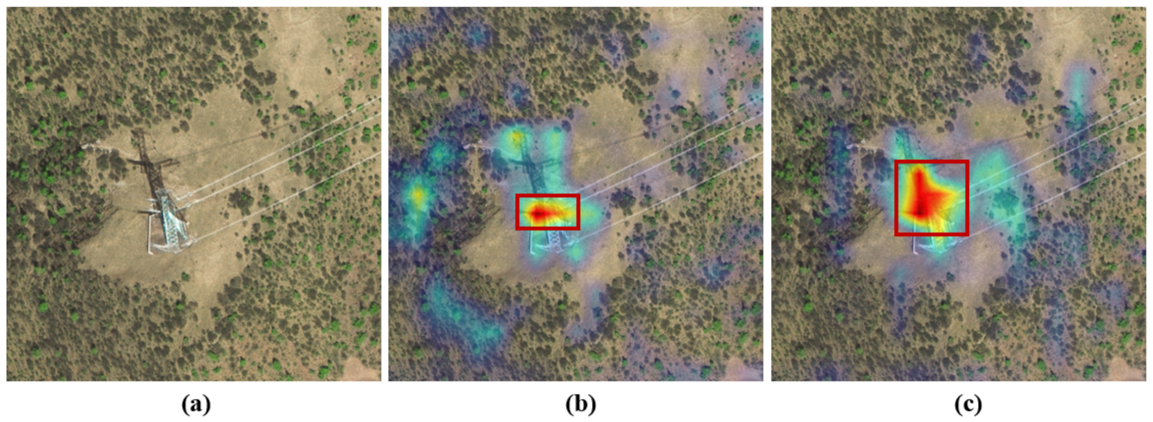
Huang et al. [22] proposed SI-STD. The network introduces shadow information to compensate for the characteristics of target lost during imaging. In the case of sufficient illumination, the problem of information loss is basically solved. It is just a preliminary attempt to use external information such as shadows for detection. It does not fully consider the impact of imaging conditions on the presentation of features, and still strongly depends on the features presented by the training data set. When the view angle changes, the generality of the algorithm model is insufficient, and the performance of the model decreases. SI-STD introduces shadow information to complement the features lost during imaging, but the generation of shadows is completely dependent on the solar elevation angle, and its performance in the image has nothing to do with the satellite perspective, while the target’s performance in the image basically depends on the satellite perspective, the roots of the shadow and the target are completely different, but SI-STD merges the shadow and the target together and treats them as a big target for detection. This approach is obviously affected by the satellite perspective. Any changes in these parameters will affect the results. As shown in Figure 1, when the satellite perspective is relatively small, the imaging information of the target in the image is not obvious. At this time, the recognition is basically based on shadow information, and when the satellite perspective is larger, the imaging information of the target in the image becomes gradually obvious. At this time, the characteristics of the shadow and the target can be considered comprehensively in the recognition. However, SI-STD merges the shadow and the target together and obviously cannot automatically assign the weight of the shadow and the target. As shown in Figure 2b, this figure is the result of the heatmap of SI-STD. The darker the color in the figure, the higher the attention of detection. It can be seen that most of the attention of SI-STD is on the target itself; there is little attention to the shadow, but the information contained in the shadow of the image is obviously greater than the target itself. This also confirms that although SI-STD can solve the problem of feature loss, there are still shortcomings when the satellite perspective changes.
In summary, the detection of high-voltage transmission towers based on optical satellite images still has the following problems:
- During imaging, a large number of features of slender targets are lost. As shown in Figure 1, for traditional object detection methods, the main features of some stumpy targets such as houses are concentrated on the top. The information will not be lost during imaging and has little effect on object detection. However, the main characteristics of slender targets such as high-voltage transmission towers are concentrated on the vertical trunk. During imaging, they will be greatly compressed in the vertical direction, and many features will be lost, which is not conducive to object detection.
- According to the imaging geometry model of the optical satellite remote sensing, the imaging results are greatly affected by the satellite perspective. The same target has different image under different satellite perspective. As shown in Figure 1a,b, high-voltage power transmission towers behave differently under different satellite perspective. In different situations, target information and shadow information contribute differently to detection.
Through the above analysis, we cannot combine the shadow with the target together. For this reason, we propose STC-Det, which treats the shadow and the tower as two types of targets to detect separately, and realize the automatic distribution of the weights of shadow information and tower information. In summary, the overall contribution of this paper is as follows:
- STC-Det is proposed, which broadens the application range of slender target detection and expands the application range of satellite perspective.
- Using deformable convolution for reference, an automatic shadow and target matching method is designed. This method achieves fast shadow and target matching with only a small increase in network complexity, improves network efficiency, and reduces computational complexity.
- A new feature fusion method is designed, which realizes the fusion of shadow features and target features, and can also realize automatic weighting of features, which further improves the utilization efficiency of shadow and target feature information.
- In order to intuitively see the influence of shadow information and target information on detection when the satellite perspective changes, we have improved Group-CAM [23] so that it can be used for the visualization of the heatmap of object detection, and thereby verify the effectiveness of STC-Det.
2. Materials and Methods
In this part, we first analyze the imaging geometry model of optical satellite images, then introduce the overall architecture of STC-Det, and the two main innovative modules AMM and FFM, and finally introduce our method for heatmap calculation.
2.1. The Imaging Geometry Model of Optical Satellite Images
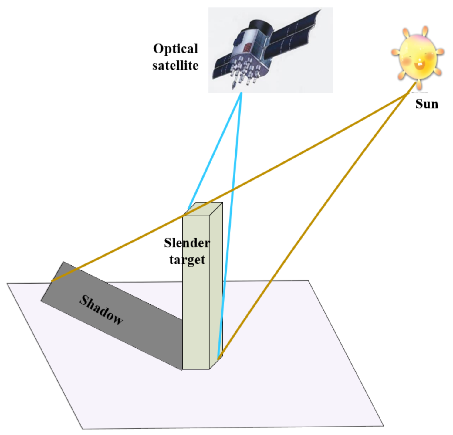
Figure 3 shows the imaging geometry model of slender targets in optical satellite images. Different from stumpy targets, the characteristics of slender targets are often distributed on the trunk located on the side elevation of the target. The optical satellite utilizes side-view imaging. When the satellite perspective is small, most of its trunk features are compressed during imaging. When the satellite perspective is not too small, some of its trunk features will inevitably be compressed. This provides different imaging results for the same slender target under a different satellite perspective. The shadow of the slender target is produced by the sun, which reflects the trunk characteristics of the target and has nothing to do with the satellite perspective. Shadows are flat features. According to the imaging model, it can be seen that the image of shadow is basically not affected by the satellite perspective. Therefore, in the case of a small satellite perspective, we can use shadow information to supplement the trunk information lost in imaging of slender targets; when the satellite perspective changes, the shadow imaging results are basically unchanged, and we can use constant shadows to assist in the detection of changing targets, thereby reducing the impact of the satellite perspective on the detection of slender targets. Based on this feature, we proposed STC-Det.
2.2. STC-Det
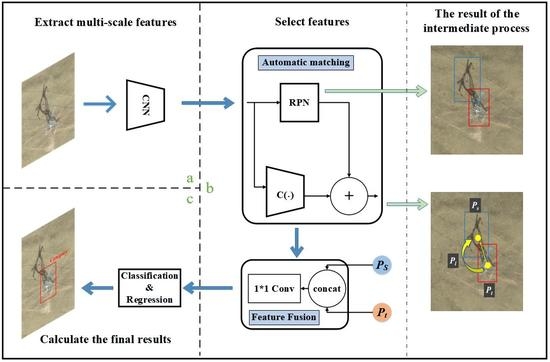
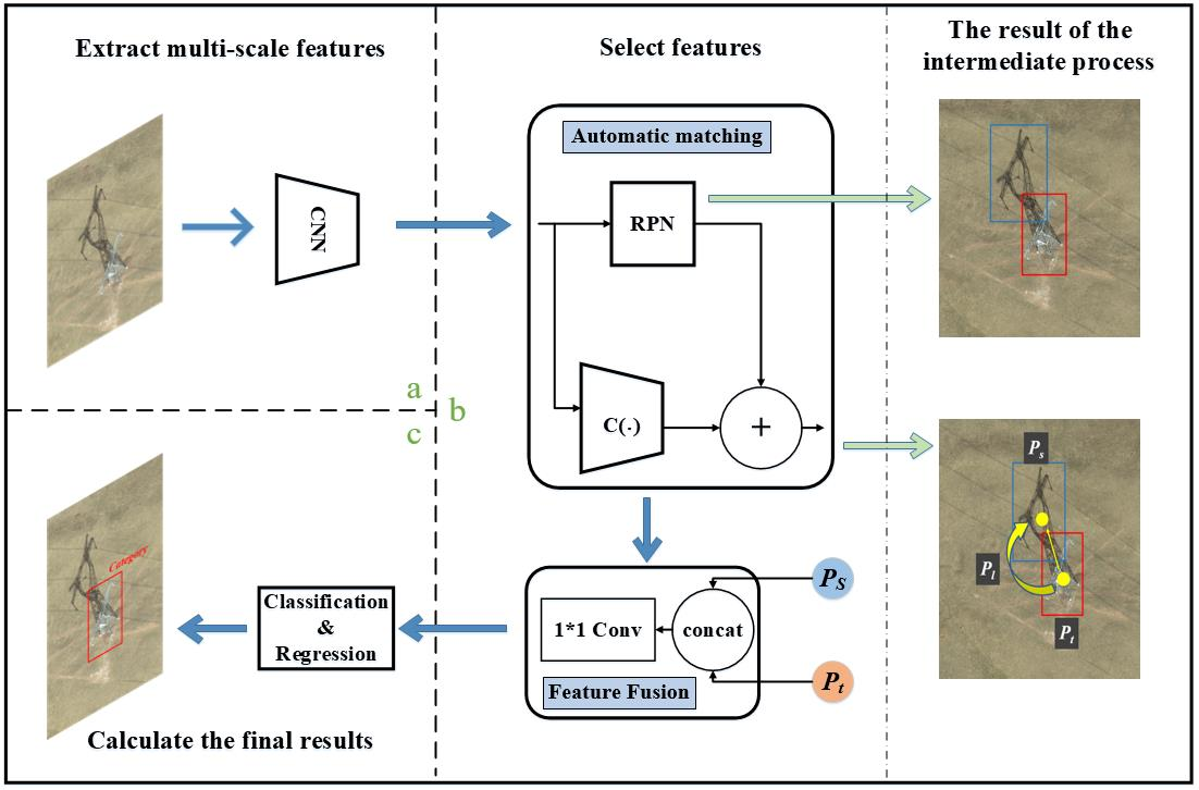
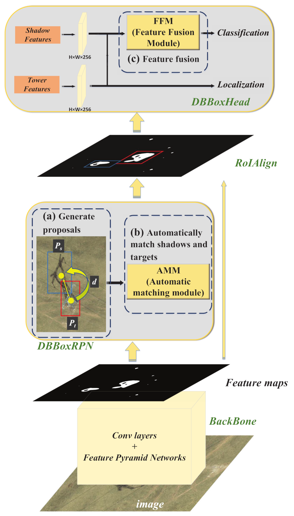
As shown in Figure 4, STC-Det still uses the structure of Faster R-CNN [17], but it improved the region proposal network (RPN) and Head in Faster R-CNN, and named them DBBoxRPN and DBBoxHead, respectively. In DBBoxRPN, the candidate regions of the shadow and the target are extracted separately, and the automatic matching module (AMM) module is used to realize the automatic matching of the shadow with the target. In DBBoxHead, the FFM module is used to realize the information fusion and automatic weighting of shadow features and target features, which solves the problem of information fusion.
In Figure 4, BackBone is mainly used to extract features of different scales of data. This part is mainly composed of ResNet [24] and FPN [25]. ResNet is a deep convolutional network, which mainly includes a convolutional layer, pooling layer, and activation layer. ResNet is used to extract features of different depths. FPN is a feature combination network that combines features extracted by ResNet into feature groups of different scales and depths. The input data of the BackBone part is the original image () after normalization and other preprocessing, , finally output a five-layer feature .
The role of DBBoxRPN is similar to that of RPN in Faster R-CNN, except that it not only needs to extract the candidate regions of the target but also needs to extract the candidate regions of the shadow corresponding to the target, as shown in Figure 4a. DBBoxRPN consists of a shared convolution layer and five convolution channels. The five layers of features extracted by BackBone are input into DBBoxRPN for calculation in turn, and all feature layers share the same set of convolution operations. The specific formula is as follows:
where , and are six convolutional layers of different sizes, , and d are respectively the confidence of the shadow candidate regions predicted by the network, the confidence of the target candidate regions, the regression of the shadow candidate regions, the regression of the target candidate regions, and the offset of the shadow relative to the target (the offset is used to realize the automatic matching of shadow and target; it will be described in detail in the following Section 2.3). , , is the regressor at the center of the prediction box, w and h are the regressions of the predicted regions width and height, respectively. , and are the offset of the shadow center of the same target relative to the x and y coordinates of the target center, respectively.
The ground truth of the shadow and target are and , respectively. The ground truth of the categories of shadow and target are and , respectively. The anchors of the shadow and target are and . The predicted proposals for shadow and target are and , respectively. They have the following relationships:
The deviations of the ground truth of the shadow and the target from the anchor are and , respectively. They can be obtained by the following equations:
After extracting the shadow and target candidate regions, the shadow and target must be matched. From the imaging geometry model, the shadow in image is related to the target. The shadow is the image of the target under the sun, and the two must be connected in space. The side-view imaging of satellite will not change this. The AMM module (described in detail in Section 2.3) uses the relationship between the shadow and the target on the image to match the extracted shadow candidate regions with the target candidate regions. DBBoxRPN outputs a series of paired proposals , among them, and are the shadow candidate regions and target candidate regions of the same target, and N is the maximum number of candidate regions extracted from a signal image.
The loss of DBBoxRPN is:
where represents the total number of extracted target candidate regions, represents the total number of extracted shadow candidate regions, represents the number of target candidate regions that can be matched to the shadow candidate regions, and represents the ground truth of the offset of the shadow center to the target center. , , and are the loss of classification, regression, and position shift, respectively. uses FocalLoss [26], the gamma and alpha of which are set to 2.0 and 0.25, respectively. and use SmoothL1Loss (as shown in Formula (15)). The weight of each loss in Formula (14) is 1.
The proposals extracted by DBBoxRPN undergo RoIAlign [27] to extract the corresponding features and , , where is an interpolation operation.
Finally, and are input into DBBoxHead for classification and regression. DBBoxHead contains two channels. One channel is used for classification; it contains a feature fusion module (FFM) and two fully connected layers. The other channel is used to regress the target position; it only contains two fully connected layers, specifically:
Among them, c represents the category results of the network, B represents the target position regression results of the network, represents the fully connected layer, represents the tiling operation, and represents the feature fusion module (described in detail in Section 2.3).
The loss of DBBoxRPN is:
where uses cross-entropy loss, and uses SmoothL1Loss (as shown in Formula (15)). The weight of each loss in Formula (18) is 1.
The total loss of the entire network is:
2.3. AMM
The automatic matching module (AMM) is located in DBBoxRPN, as shown in Figure 4b, which is used to match the extracted shadow candidate regions with target candidate regions. Generally, if you want to match the shadow and target together, you must use the position information of the two. Although preliminary matching can be carried out, it needs to be matched and screened one by one. The speed is slow, and the error of using the position information to match is also relatively large. AMM can easily and quickly match the shadow candidate regions with target candidate regions.
Figure 5b is a schematic diagram of deformable convolution. Deformable convolution calculates the position offset of each position to change the receptive field of the convolution kernel, so as to realize the convolution of any shape. Deformable convolution can be calculated by the following formula:
where f represents the feature before convolution, F represents the feature after convolution, and represents the offset of each feature point , which can be learned through the network.
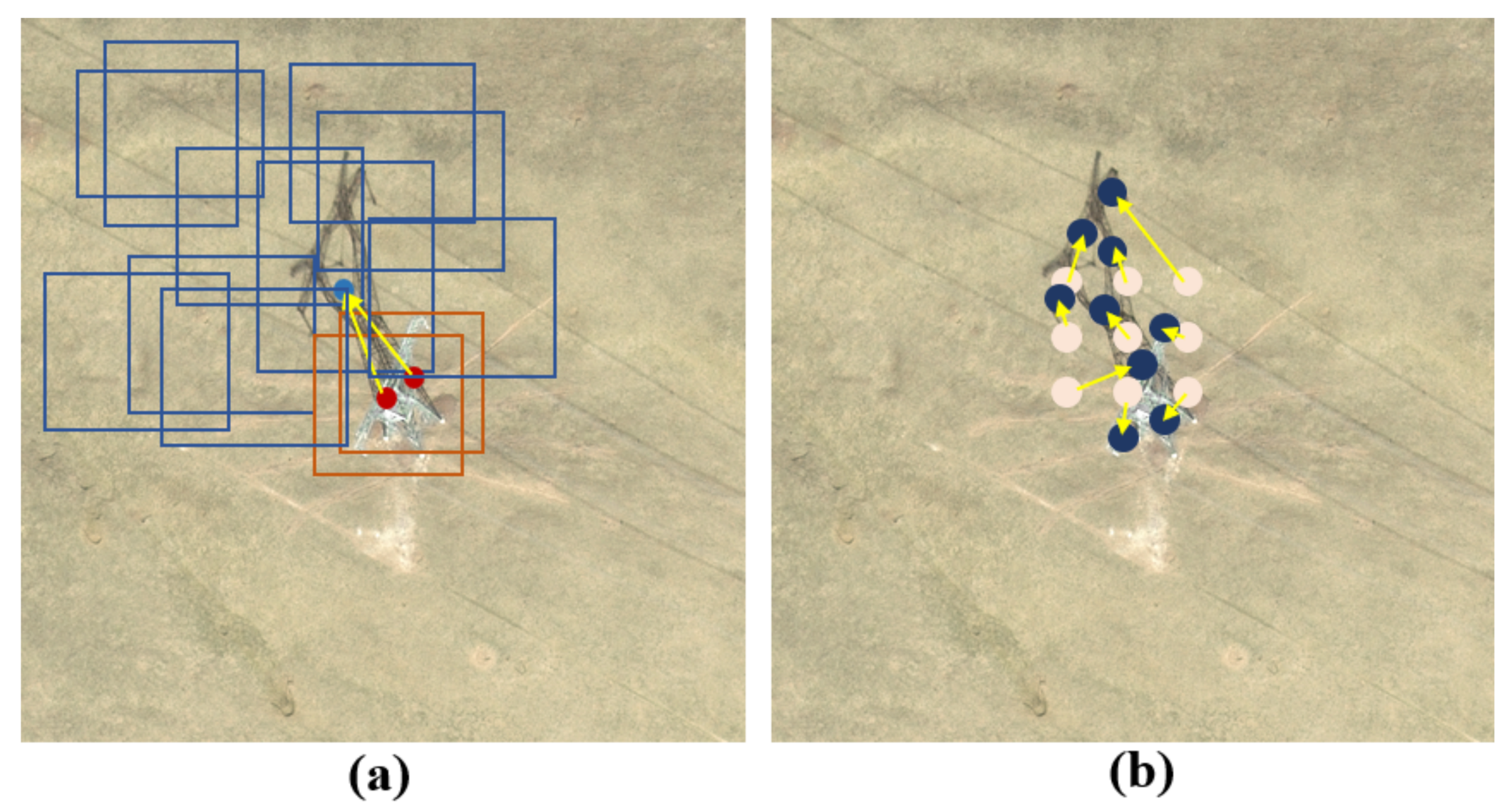
Deformable convolution [28] obtains the offset of each feature point through the network, which can realize the convolution of any shape. Deformable convolution learns the mapping of the convolution kernel to different parts of the target. According to the imaging geometry model of the optical satellite, the same pair of target and shadow should be connected together. If the target and shadow are regarded as a whole, the target and shadow will be two parts of the whole. Drawing lessons from the idea of deformable convolution, we designed AMM. We can directly learn the mapping from the center of the target to the center of the shadow, which is equivalent to learning the mapping of two parts. With this mapping, we can directly map the target candidate regions to the position of the shadow candidate regions and quickly achieve the matching of the candidate regions. As shown in Figure 5a, the blue rectangle in the figure represents the candidate regions of the shadow, the red rectangle represents the candidate regions of the target, the blue dot represents the center point of the shadow, and the red dot represents the center point of the target. According to the mapping from the target to the shadow, we can directly get the shadow center point from the target candidate region. If the center point of the shadow candidate region is consistent with the obtained shadow center point, the corresponding shadow candidate regions matches the target candidate regions. The specific calculation is shown below.
The calculation of the offset d from the target center to the shadow center is shown in Section 2.1. The ground truth of the center offset is :
When matching the shadow with target, according to the target candidate region , the matching shadow center can be obtained by the center offset :
Through the above calculations, we obtain the shadow center and the predicted shadow candidate region . We only need to find the corresponding shadow prediction regions according to the calculated shadow center . If there is a shadow prediction region centered on , then is the shadow prediction region that matches the target prediction region .
In training, both the predicted regions of the target and the shadow are different from the ground truths. To improve robustness, after the shadow center is obtained, is not directly compared with the center of the shadow prediction region. We first calculate the center of the shadow prediction region. If the center of the shadow prediction region falls within a certain range centered on , it can be regarded as a matching candidate region, and then select the one with greatest confidence from these candidate regions as the final result.
2.4. FFM
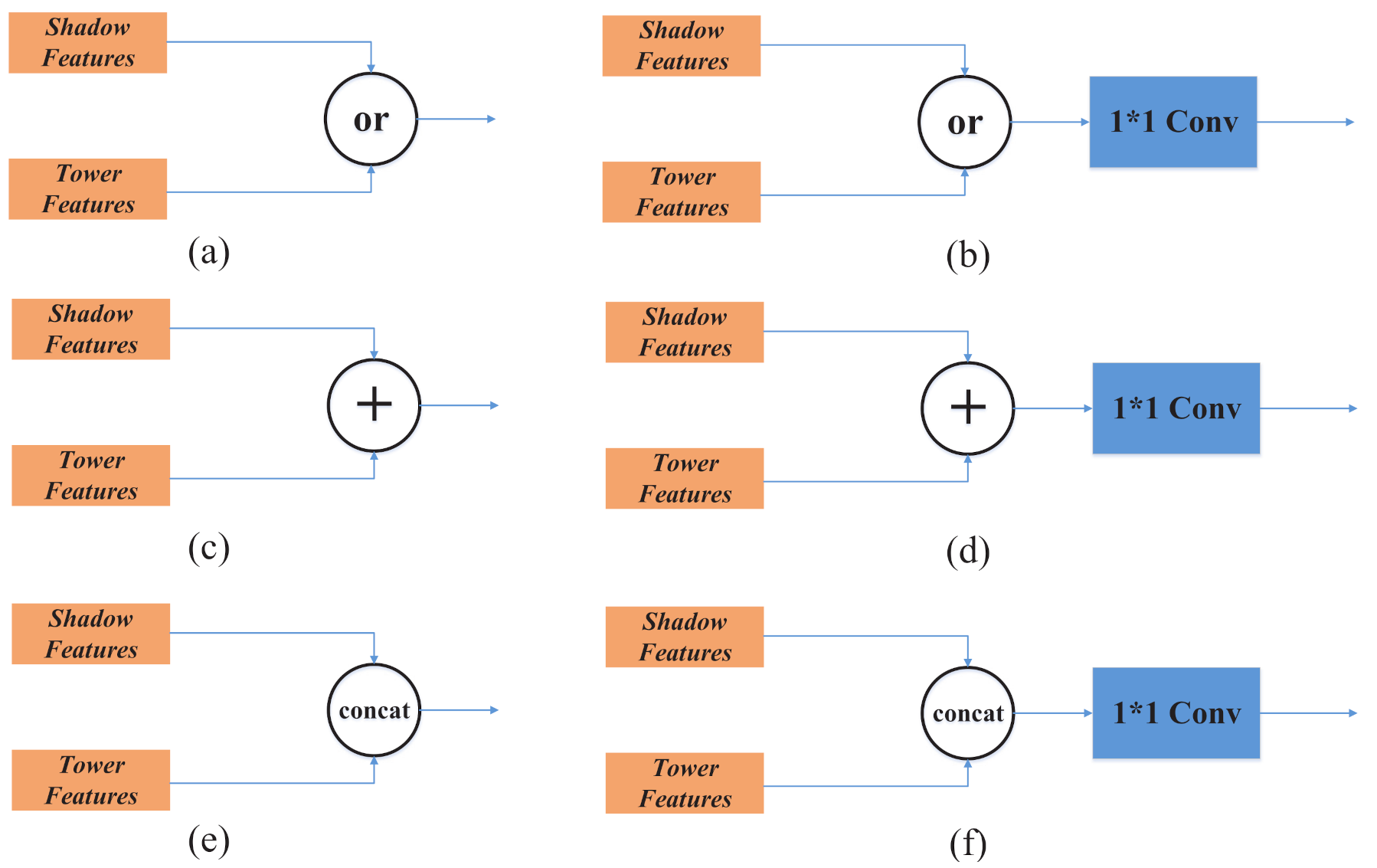
The feature fusion module (FFM) is located in DBBoxHead (as shown in Figure 4c), and its main function is to fuse the features of classification. DBBoxRPN not only extracts the candidate regions of the target but also extracts the shadow candidate regions corresponding to the target. When classifying, we can use only the shadow feature, or only the target feature, or even use the combined features of the two at the same time and automatically set the weight of the difference, as shown in Figure 6. From the analysis of satellite imaging geometric model, when satellite perspective are small, the characteristics of the target are not too obvious, and the shadow information is more obvious, so the shadow information can be used for classification. Theoretically, as long as the fusion weights of the two types of features are reasonably allocated for classification, the combined use of the features of the target and the shadow for classification will have a better effect. For this reason, we designed the FFM module to perform feature selection and fusion.
Figure 6 shows six feature fusion methods, of which (a) and (b) use only one feature of the shadow and the target, (c) and (d) directly add the shadow and the target feature together, and (e) and (f) combine the features of the shadows and the target. The three fusion methods on the left in Figure 6 do not use 1*1 convolution after fusion, while the three methods on the right use 1*1 convolution after fusion. 1*1 convolution is a point-by-point channel convolution, where it acts as a weighted average and can dynamically learn weighting coefficients.
After the above theoretical analysis and comparative experiments (Table 1), we choose Figure 6f as the FFM module, which is specifically:
Among them, , , and represent the extracted shadow features, target features, and the output of FFM, respectively. stands for feature stacking operation, and stands for 1*1 convolution operation.
2.5. Heatmap Visualization Algorithm
Group-CAM is a heatmap visualization algorithm for image classification. We have improved Group-CAM to enable it to be used for object detection. The calculation of Group-CAM is divided into four steps:
- Input the original image into the network F and extract the characteristic layer A and the corresponding gradient value W to be viewed.
- Use filter to filter the original image to get , use the extracted gradient value W to weight the feature layer A and group to get the feature mask , L is to be divided into a number of groups.
- The feature mask M is respectively weighted and merged with the original image after the illusion, and the masked image I is obtained. Input I into the network to obtain the weight of the corresponding feature layer.
- Use the obtained feature layer weights to weight the corresponding feature layers to obtain the final heat map.
In image classification, the confidence score of the corresponding category of the data can be obtained by inputting the data into network, and the score can be directly used as the weight. In object detection, the data input into network can obtain a series of prediction regions and confidence. The result cannot be used directly as a weight.
In order to make Group-CAM suitable for object detection tasks, we made adjustments in the third step of the original Group-CAM. When calculating the weight in the third step, we do not directly use the final result but use the loss of the corresponding data as the weight, and the loss is just the opposite of the original confidence. The greater the confidence of the original Group-CAM, the greater the weight. Here, the greater the loss, the smaller the weight, specifically:
3. Experiment
3.1. Data Set
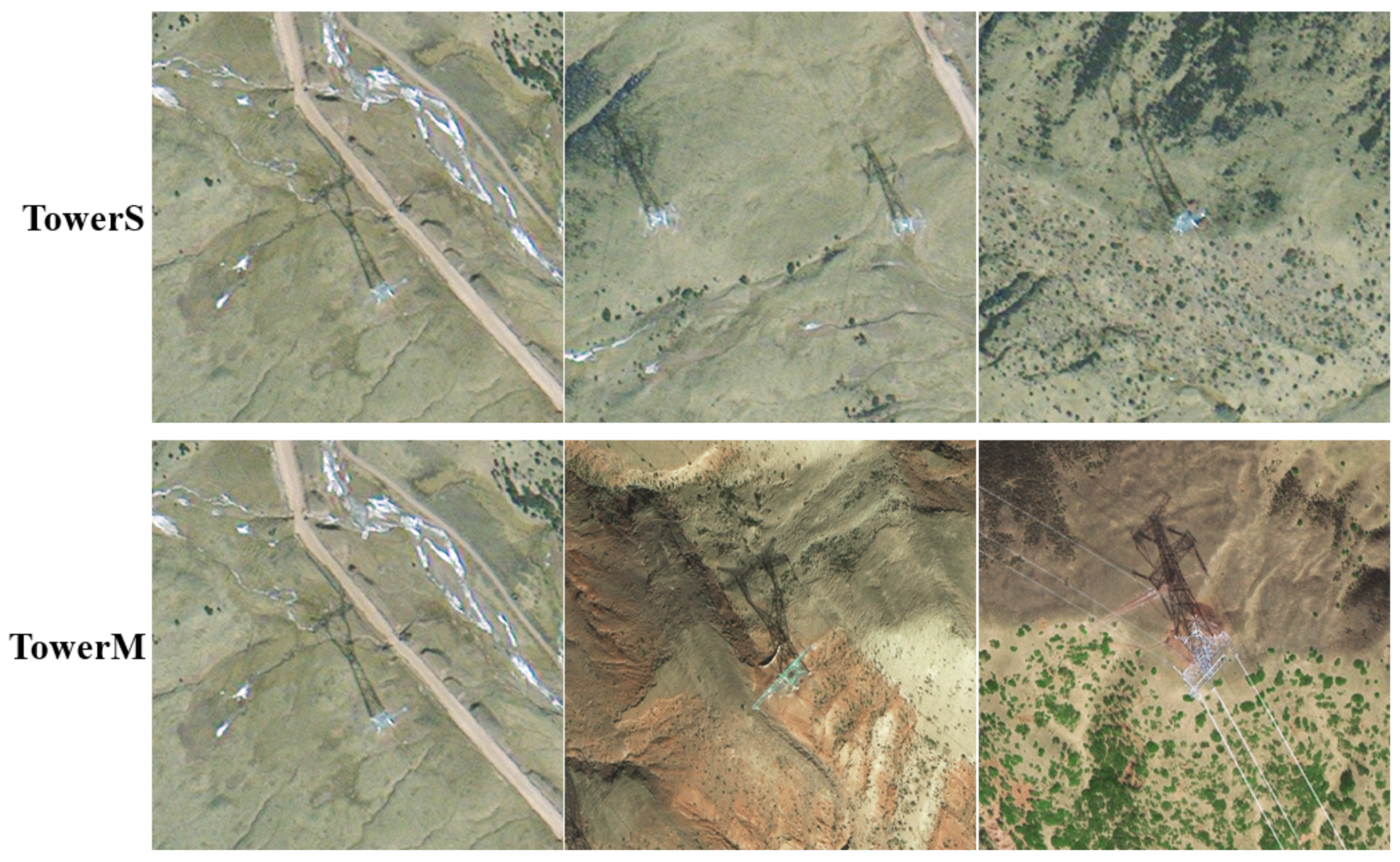
The data used in the experiment includes three types of transmission towers with heights between 15 m and 70 m, namely the wine-glass tower, the dry-type tower and cat-head tower, the same as SI-STD [22]. In order to verify the effectiveness of the methods proposed in this paper, we made two data sets. To make it easier to distinguish, we named the first data set “TowerS” and the second data set “TowerM”, as shown in Figure 7. The satellite perspective of TowerS is relatively small, and the satellite perspective of TowerM is variable. Both of these data sets are intercepted from BJ-2, WV-2 and Google Earth, and the size of a single data is 600*600. TowerS contains 1574 training data and 686 test data, while TowerM contains 2575 training data and 904 test data. The data volume of the three towers in all data sets is approximately 1:1:1.
3.2. Training Configurations
All experiments in this paper are carried out in the PyTorch environment. The experimental platform is two RTX 2080 Ti graphics cards, and the batch size is set to 4. The size of the experimental optical images is 600*600. In order to facilitate subsequent operations, it is filled with 0 to 608*608. There are a total of 20 epochs in the experiment. The initial stage learning rate is set to 0.001667. In the following 3600 steps, the learning rate increases by at each step until it increases to 0.005. From the seventh to the twelfth epoch, the learning rate drops to 0.0005, and from the thirteenth to the twentieth epoch, the learning rate drops to 0.00005. In the DBBoxRPN part, the network uses an anchor-based method to extract the shadow and target candidate regions. There are 16 shadow anchors, the aspect ratio is [1.0,2.0,3.0,4.0], and the scale size is [4,8,16,32], 12 anchors of the target are set, the aspect ratio is [0.5,1.0,2.0,3.0], and the scale size is [4,8,16,32]. Shadow and target are in progress. When matching, the and in Equations (21)–(24) are 50. In order to improve the robustness of matching, after calculating the center position of the predicted shadow regions, we will perform matching within a radius of 50 (This value is determined through experiments, as shown in Figure 8.).
3.3. Parameter Selection and Ablation Experiment
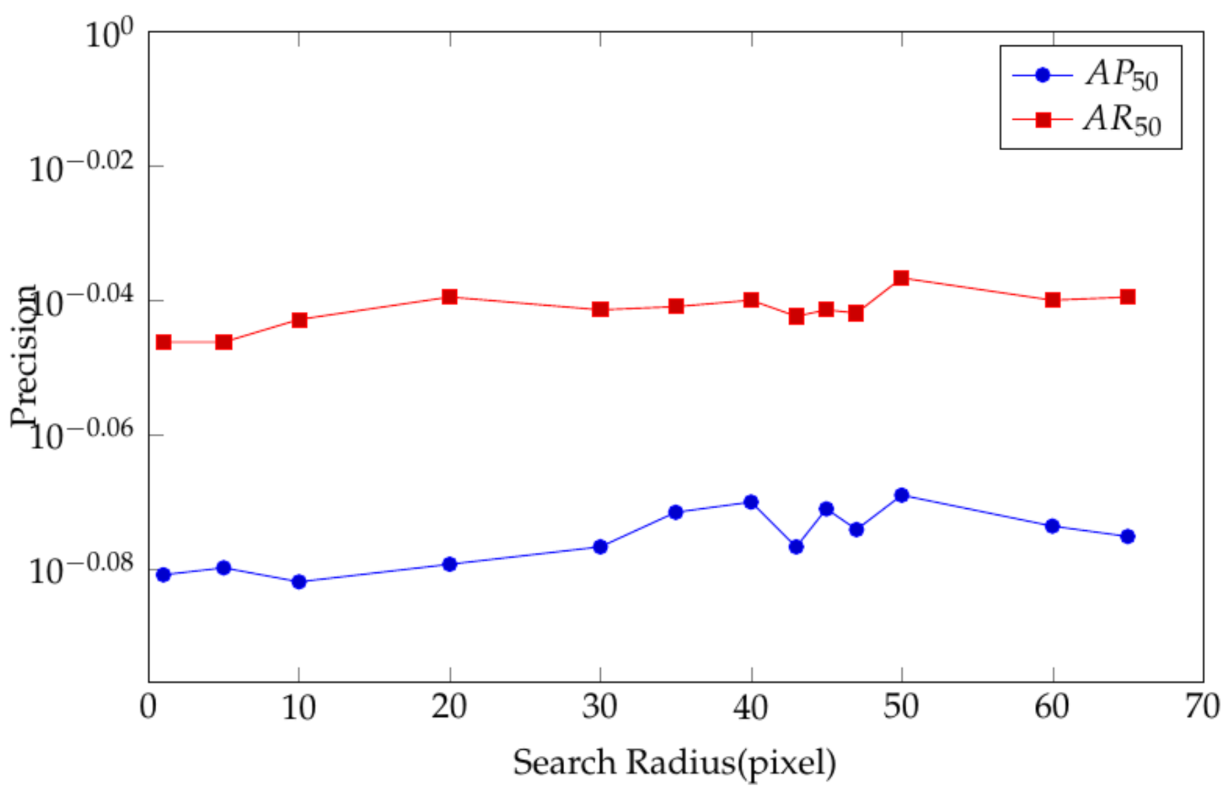
In AMM of the DBBoxRPN part, when matching the shadow with the target, we use the tower as the target to find the corresponding shadow. According to the center of the target candidate region and the offset from the target to the shadow, we can get the position of the shadow center . At this time, the shadow candidate region with as the center can be directly selected as the shadow to be matched, but there are some deviations. The shadow candidate regions and target candidate regions predicted by the network have a certain deviation from the ground truth, and there will be a certain error in directly using the shadow candidate regions. In order to reduce errors and improve the robustness of the network, we do not directly use as the shadow center but regard the shadow candidate regions within a certain range of the circle center as the possible range of the shadow to be matched and then select the shadow candidate with the highest confidence in this range as the matching shadow. The search range is a hyperparameter. In order to find the optimal range, we have conducted a series of experiments for different search ranges, as shown in Figure 8. Through experiments, it is found that the precision of the result is highest when is the center of the circle and the search radius is 50. This value is also used in subsequent experiments.
In FFM of the DBBoxHead part, we propose several feature fusion methods, as shown in Figure 6. In order to choose the best method, we conducted further experiments on these methods. The experimental results are shown in Table 1. In this table, “shadow” means that only shadow information is used, “tower” means that only target information is used, and “add” and “concat” mean that both shadow and target information are used together. It can be seen that only using shadows for classification has the lowest precision, followed by only using targets for classification. The precision of classification using shadow and target information is higher than that of using only one type of information alone. This also proves that our idea of using shadows to complete actual information and to assist classification is correct. Judging from the postoperation without using convolution, in addition to using shadow information alone for classification, other methods have improved accuracy after using convolution. convolution is also equivalent to a weight allocator, indicating that it is effective to redistribute feature weights before classification.
The result in row 3 in Table 1 is the result when only the target information is used for classification and no postoperation is performed. This experiment just divides the classification and regression of the Head part in the original Faster R-CNN framework into two channels for processing separately. Comparing the results of Faster R-CNN in Table 2, it can be seen that in the final classification, separating classification and regression can improve the precision and reduce the mutual influence of classification and regression. Comparing the results of the first four rows with the last four rows of Table 1, it can be seen that the comprehensive use of shadow and target information for classification can indeed improve the final precision. This also reflects that our AMM is indeed effective and can accurately match the shadow to the target.
3.4. Results
3.4.1. Performance on the Two Data Sets
In the experiment part, there are five comparison networks, namely Faster R-CNN [17], TSD [29], ATSS [30], Retinanet [26], and SI-STD [22]. In order to verify the effectiveness of STC-Det when the satellite perspective change, we establish two data sets, which are called TowerS and TowerM, respectively. The satellite perspective of the data in TowerS are relatively simple, while the satellite perspective of the data in TowerM are variable. There are six experimental indicators: “”, “”, “”, “”, “”, “”. “”, “”, “” represent the precision of networks under different IoU thresholds, “” represents the average recall of networks under different sizes of bboxes, “” represents the number of network parameters, “” represents the network’s ability to process data per second, the calculations of “Precision” and “Recall” are shown in Formula (33) and (34), and the calculation method of the above six parameters is consistent with the MS COCO data set [31]. The performance of experimental networks on the two data sets are shown in Table 2 and Table 3, respectively.
Through the analysis of Table 2 and Table 3, it can be seen that the precision of STC-Det on the TowerS data set is increased by 5.2% compared with other networks, and the precision on the TowerM data set is still improved by 1.7% compared with other networks (here, considering the average precision ). On the TowerS data set, the recall of STC-Det increased by 1.6%, and it also maintained a high recall rate on the TowerM data set. However, the network parameters of STC-Det did not increase much, much less than the number of parameters of TSD, indicating that STC-Det improved the detection precision while maintaining no significant increase in parameters. Observing the FPS index, it is found that the detection speed of STC-Det is the slowest among these networks, almost twice as slow as other networks. This is because the network needs to extract the shadow and target candidate regions at the same time, and also to match the shadow and the target, which undoubtedly greatly increases the amount of calculation, but in the case of low requirements for detection speed, it is worthwhile to trade the loss of detection speed for a substantial increase in precision.
3.4.2. Visualization of Results
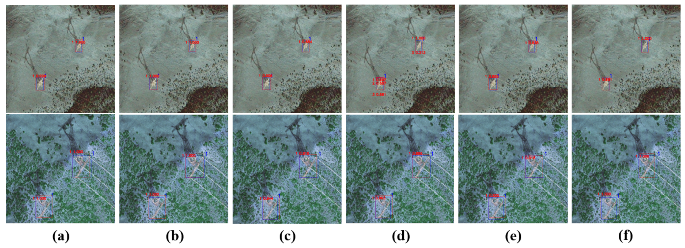
Figure 9 shows the visualization results of the networks used in the experimental part. Combining Table 2 with Table 3, it can be seen that these networks can all complete the detection task. Networks such as Faster R-CNN, TSD, ATSS, and Retinanet perform relatively ordinarily on these two data sets. SI-STD performs better when the satellite perspective is small, while the precision decreases when the satellite perspective increases. This may be due to the increase of the satellite perspective, and the target features gradually become obvious. SI-STD basically only pays attention to the target, so the shadow next to target will interfere with the detection. STC-Det performed well in both cases, which may be due to the separate use of shadow and target features and the different weights of shadow and target.
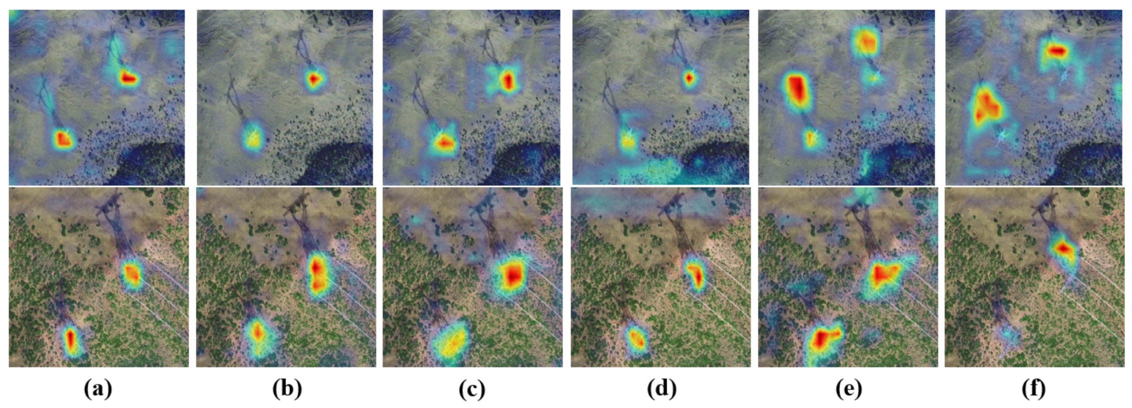
Figure 10 can also explain this phenomenon. It can be seen from the heatmap that traditional networks such as Faster R-CNN, TSD, ATSS, Retinanet pay more attention to the target itself. These networks only focus on the target itself and ignore the shadows next to the target. When the satellite perspective is small, the characteristics of the target are very inconspicuous, which makes the detection precision low. After the satellite perspective is increased, the target features are obvious, and the detection precision is improved. According to Figure 10e, it can be seen that when the satellite perspective is small, the SI-STD pays attention to the shadow and the target at the same time. At this time, the target characteristics are not obvious, and the network tends to shadow characteristics. This phenomenon makes sense. But when the satellite perspective increases, the target characteristics become obvious. SI-STD almost only pays attention to the target feature, but it also extracts the shadow feature. The shadow extracted interferes with the overall detection and reduces the detection precision. It can be seen from Figure 10f that STC-Det can comprehensively use shadow features and target features regardless of whether the satellite perspective is large or small. It can be clearly found that when the satellite perspective is small, STC-Det pays more attention to the shadow features. When the satellite perspective is large, STC-Det is more inclined to focus on the target features, which is also our expectation. It can be proved that compared with SI-STD, STC-Det can flexibly set different weights for shadows and target features, and can automatically select different degrees of attention in different situations, which also broadens the scope of application of the network to the satellite perspective.
3.5. Discussion
The trunk information of the slender target in the optical satellite remote sensing will be greatly compressed during imaging, and its performance is greatly affected by the satellite perspective. In most cases, the shadow of a slender target can well reflect the missing structural features of target, and the imaging of the shadow is basically not affected by the satellite perspective. Based on this feature, we designed the STC-Det network, which uses shadow information to assist in detecting slender targets, and can automatically adjust the weights of shadows and targets under different satellite perspective, which greatly improves the detection accuracy and the robustness of the satellite perspective. SI-STD is our preliminary attempt to detect slender targets based on shadow information. Based on SI-STD, STC-Det is proposed to solve the impact of satellite perspective on detection. However, there are still some problems that need to be overcome. First, the shadow-based detection methods are greatly affected by shadows. In some extreme weather or special solar parameters, the shadow information is blurred, which not only cannot help the detection, but will interfere with the detection. Second, the current method uses less external information such as satellite parameters and is a completely data-driven detector, which requires a great amount of data and calculations, and the detection efficiency of the algorithm is low. To solve this problem, we can consider adding external prior information such as satellite parameters in the to reduce the dependence on data and the complexity of algorithm. Finally, the existing research does not consider the drastic changes of the solar altitude and the solar azimuth, which is also a problem that needs to be overcome in the future.
4. Conclusions
In this paper, we found that there are two problems in the detection of slender targets based on optical satellite images. One is that the main feature of slender targets located on the side elevation of the trunk is compressed greatly during imaging, which is not conducive to detection. Second, the performance of slender targets such as power transmission towers in the image is greatly affected by the satellite perspective, and the same target behaves completely differently under different satellite perspectives. In response to these two problems, this paper has made some improvements. We analyzed the imaging geometry model of slender targets and their shadows in optical satellite images. Slender targets are easily affected by changes of the satellite perspective, while their shadows are less affected by the satellite perspective. When the satellite perspective is small, shadows can be used to make up for the missing side elevation shape information of the slender targets. When the satellite perspective changes, the invariable shadow features can be used to assist in the interpretation of the changing slender targets. Combining this idea, in the paper, we propose STC-Det. STC-Det imitated deformable convolution and designed the AMM module to realize the automatic matching of the shadow candidate regions with the target candidate regions, and the FFM module was proposed after many experiments to effectively use the shadow and target information, which realized the fusion of shadow and target information and the automatic distribution of the weights of the two. Finally, in order to intuitively see the impact of changes in satellite perspective on slender targets and shadow imaging results, in this paper, we improve the existing heatmap algorithm to make it suitable for object detection and verify the validity and correctness of the method proposed in the paper in an intuitive way. In this paper, we propose a series of improvement measures for the detection of high-voltage power transmission towers and other slender targets in optical satellite images. These methods are indeed effective, but there are still many shortcomings. Some hyperparameters of the STC-Det network proposed in this paper need to be adjusted manually, and the detection speed of the network needs to be improved. Therefore, the focus of the next phase of work is to reduce the number of hyperparameters in the network and improve the efficiency of the network.
Author Contributions
Z.H. and F.W. designed the algorithm; Z.H. performed the algorithm with Python; H.Y. and Y.H. guided the whole project; Z.H. and F.W. wrote this paper; H.Y. and F.W. read and revised this paper. All authors have read and agreed to the published version of the manuscript.
Funding
This research received no external funding.
Institutional Review Board Statement
Not applicable.
Informed Consent Statement
Not applicable.
Data Availability Statement
The data that support the findings of this study are available from the corresponding author upon reasonable request.
Conflicts of Interest
The authors declare no conflict of interest.
References
- Rostami, M.; Kolouri, S.; Eaton, E.; Kim, K. SAR Image Classification Using Few-Shot Cross-Domain Transfer Learning. In Proceedings of the 2019 IEEE/CVF Conference on Computer Vision and Pattern Recognition Workshops (CVPRW), Long Beach, CA, USA, 16–20 June 2019. [Google Scholar]
- Xu, D.; Wu, Y. Improved YOLO-V3 with DenseNet for Multi-Scale Remote Sensing Target Detection. Sensors 2020, 20, 4276. [Google Scholar] [CrossRef]
- Nie, X.; Duan, M.; Ding, H.; Hu, B.; Wong, E.K. Attention Mask R-CNN for ship detection and segmentation from remote sensing images. IEEE Access 2020, 8, 9325–9334. [Google Scholar] [CrossRef]
- Yin, S.; Li, H.; Teng, L. Airport Detection Based on Improved Faster RCNN in Large Scale Remote Sensing Images. Sens. Imaging 2020, 21, 49. [Google Scholar] [CrossRef]
- Wu, L.; Ma, Y.; Fan, F.; Wu, M.; Huang, J. A Double-Neighborhood Gradient Method for Infrared Small Target Detection. IEEE Geosci. Remote Sens. Lett. 2021, 18, 1476–1480. [Google Scholar] [CrossRef]
- Sun, X.; Huang, Q.; Jiang, L.J.; Pong, P.W.T. Overhead High-Voltage Transmission-Line Current Monitoring by Magnetoresistive Sensors and Current Source Reconstruction at Transmission Tower. IEEE Trans. Magn. 2014, 50, 1–5. [Google Scholar] [CrossRef] [Green Version]
- Tragulnuch, P.; Kasetkasem, T.; Isshiki, T.; Chanvimaluang, T.; Ingprasert, S. High Voltage Transmission Tower Identification in an Aerial Video Sequence using Object-Based Image Classification with Geometry Information. In Proceedings of the 2018 15th International Conference on Electrical Engineering/Electronics, Computer, Telecommunications and Information Technology (ECTI-CON), Chiang Rai, Thailand, 18–21 July 2018; pp. 473–476. [Google Scholar] [CrossRef]
- Zhao, J.; Zhao, T.; Jiang, N.Q. Power transmission tower type determining method based on aerial image analysis. In Proceedings of the CICED 2010 Proceedings, Nanjing, China, 13–16 September 2010; pp. 1–5. [Google Scholar]
- Li, Z.; Mu, S.; Li, J.; Wang, W.; Liu, Y. Transmission line intelligent inspection central control and mass data processing system and application based on UAV. In Proceedings of the 2016 4th International Conference on Applied Robotics for the Power Industry (CARPI), Jinan, China, 11–13 October 2016; pp. 1–5. [Google Scholar] [CrossRef]
- He, T.; Zeng, Y.; Hu, Z. Research of Multi-Rotor UAVs Detailed Autonomous Inspection Technology of Transmission Lines Based on Route Planning. IEEE Access 2019, 7, 114955–114965. [Google Scholar] [CrossRef]
- Liu, Z.; Wang, X.; Liu, Y. Application of Unmanned Aerial Vehicle Hangar in Transmission Tower Inspection Considering the Risk Probabilities of Steel Towers. IEEE Access 2019, 7, 159048–159057. [Google Scholar] [CrossRef]
- Shajahan, N.M.; Kuruvila, T.; Kumar, A.S.; Davis, D. Automated Inspection of Monopole Tower Using Drones and Computer Vision. In Proceedings of the 2019 2nd International Conference on Intelligent Autonomous Systems (ICoIAS), Singapore, 28 February–2 March 2019; pp. 187–192. [Google Scholar] [CrossRef]
- Chen, D.Q.; Guo, X.H.; Huang, P.; Li, F.H. Safety Distance Analysis of 500kV Transmission Line Tower UAV Patrol Inspection. IEEE Lett. Electromagn. Compat. Pract. Appl. 2020, 2, 124–128. [Google Scholar] [CrossRef]
- IEEE Guide for Unmanned Aerial Vehicle-Based Patrol Inspection System for Transmission Lines. IEEE Std 2821-2020. [CrossRef]
- Tragulnuch, P.; Chanvimaluang, T.; Kasetkasem, T.; Ingprasert, S.; Isshiki, T. High Voltage Transmission Tower Detection and Tracking in Aerial Video Sequence using Object-Based Image Classification. In Proceedings of the 2018 International Conference on Embedded Systems and Intelligent Technology International Conference on Information and Communication Technology for Embedded Systems (ICESIT-ICICTES), Khon Kaen, Thailand, 7–9 May 2018; pp. 1–4. [Google Scholar] [CrossRef]
- Wang, H.; Yang, G.; Li, E.; Tian, Y.; Zhao, M.; Liang, Z. High-Voltage Power Transmission Tower Detection Based on Faster R-CNN and YOLO-V3. In Proceedings of the 2019 Chinese Control Conference (CCC), Guangzhou, China, 27–30 July 2019; pp. 8750–8755. [Google Scholar] [CrossRef]
- Ren, S.; He, K.; Girshick, R.; Sun, J. Faster R-CNN: Towards Real-Time Object Detection with Region Proposal Networks. IEEE Trans. Pattern Anal. Mach. Intell. 2017, 39, 1137–1149. [Google Scholar] [CrossRef] [PubMed] [Green Version]
- Redmon, J.; Farhadi, A. YOLOv3: An Incremental Improvement. arXiv 2018, arXiv:1804.02767. [Google Scholar]
- Zhou, X.; Liu, X.; Chen, Q.; Zhang, Z. Power Transmission Tower CFAR Detection Algorithm Based on Integrated Superpixel Window and Adaptive Statistical Model. In Proceedings of the IGARSS 2019—2019 IEEE International Geoscience and Remote Sensing Symposium, Yokohama, Japan, 28 July–2 August 2019; pp. 2326–2329. [Google Scholar] [CrossRef]
- Wenhao, O.U.; Yang, Z.; Zhao, B.B.; Fei, X.Z.; Yang, G. Research on Automatic Extraction Technology of Power Transmission Tower Based on SAR Image and Deep Learning Technology. In Proceedings of the 2019 6th International Conference on Information Science and Control Engineering (ICISCE), Shanghai, China, 20–22 December 2019. [Google Scholar]
- Tian, G.; Meng, S.; Bai, X.; Liu, L.; Zhi, Y.; Zhao, B.; Meng, L. Research on Monitoring and Auxiliary Audit Strategy of Transmission Line Construction Progress Based on Satellite Remote Sensing and Deep Learning. In Proceedings of the 2020 2nd International Conference on Information Technology and Computer Application (ITCA), Guangzhou, China, 18–20 December 2020; pp. 73–78. [Google Scholar] [CrossRef]
- Huang, Z.; Wang, F.; You, H.; Hu, Y. Shadow Information-Based Slender Targets Detection Method in Optical Satellite Images. IEEE Geosci. Remote Sens. Lett. 2021, 1–5. [Google Scholar] [CrossRef]
- Zhang, Q.; Rao, L.; Yang, Y. Group-CAM: Group Score-Weighted Visual Explanations for Deep Convolutional Networks. arXiv 2021, arXiv:2103.13859. [Google Scholar]
- He, K.; Zhang, X.; Ren, S.; Sun, J. Deep Residual Learning for Image Recognition. In Proceedings of the 2016 IEEE Conference on Computer Vision and Pattern Recognition (CVPR), Las Vegas, NV, USA, 27–30 June 2016. [Google Scholar]
- Lin, T.-Y.; Dollár, P.; Girshick, R.; He, K.; Hariharan, B.; Belongie, S. Feature Pyramid Networks for Object Detection. arXiv 2016, arXiv:1612.03144. [Google Scholar]
- Lin, T.Y.; Goyal, P.; Girshick, R.; He, K.; Dollár, P. Focal Loss for Dense Object Detection. In Proceedings of the 2017 IEEE International Conference on Computer Vision (ICCV), Venice, Italy, 22–29 October 2017; pp. 2999–3007. [Google Scholar]
- He, K.; Gkioxari, G.; Dollár, P.; Girshick, R. Mask R-CNN. IEEE Trans. Pattern Anal. Mach. Intell. 2017, 2980–2988. [Google Scholar] [CrossRef]
- Dai, J.; Qi, H.; Xiong, Y.; Li, Y.; Zhang, G.; Hu, H.; Wei, Y. Deformable Convolutional Networks. In Proceedings of the 2017 IEEE International Conference on Computer Vision (ICCV), Venice, Italy, 22–29 October 2017; pp. 764–773. [Google Scholar] [CrossRef] [Green Version]
- Song, G.; Liu, Y.; Wang, X. Revisiting the Sibling Head in Object Detector. arXiv 2020, arXiv:2003.07540. [Google Scholar]
- Zhang, S.; Chi, C.; Yao, Y.; Lei, Z.; Li, S.Z. Bridging the Gap Between Anchor-Based and Anchor-Free Detection via Adaptive Training Sample Selection. In Proceedings of the 2020 IEEE/CVF Conference on Computer Vision and Pattern Recognition (CVPR), Seattle, WA, USA, 16–18 June 2020. [Google Scholar]
- Lin, T.Y.; Maire, M.; Belongie, S.; Hays, J.; Zitnick, C.L. Microsoft COCO: Common Objects in Context. In Proceedings of the European Conference on Computer Vision, Zurich, Switzerland, 6–12 September 2014. [Google Scholar]
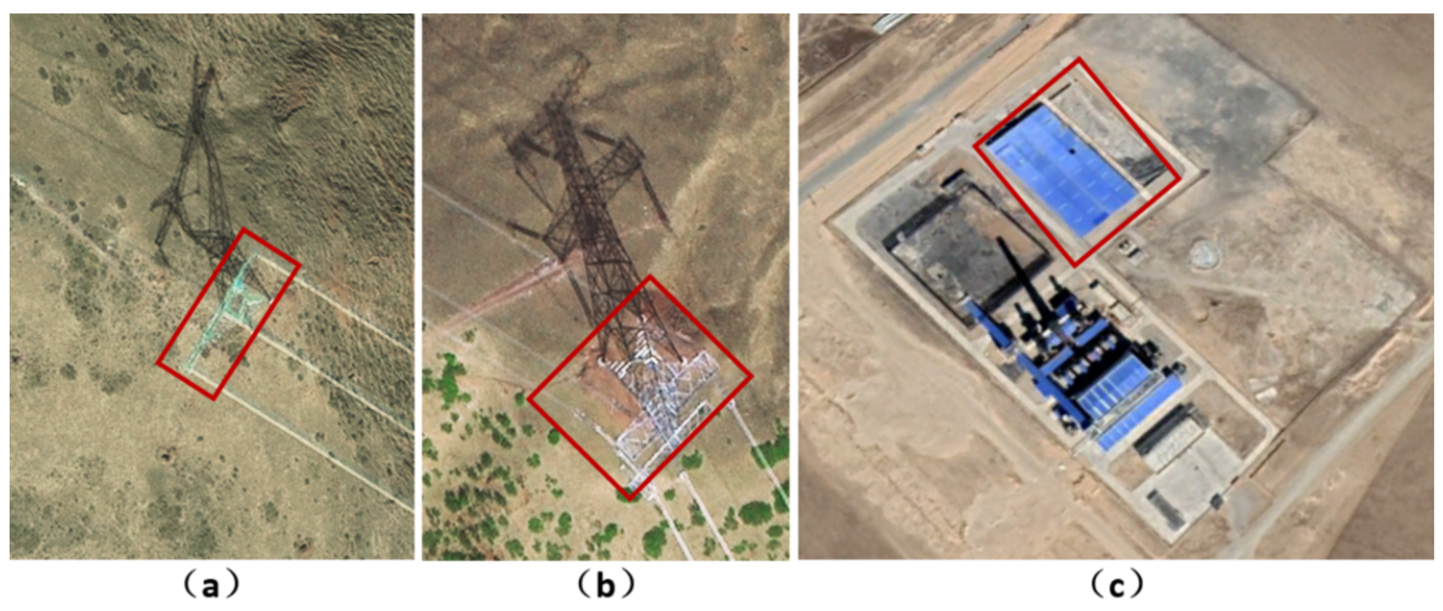
Figure 1.
Images of different types of targets in different satellite perspectives. (a) is the image of slender target in a small satellite perspective. (b) is the image of slender target in a big satellite perspective. (c) is the image of stumpy targets such as buildings.
Figure 1.
Images of different types of targets in different satellite perspectives. (a) is the image of slender target in a small satellite perspective. (b) is the image of slender target in a big satellite perspective. (c) is the image of stumpy targets such as buildings.

Figure 2.
Visualization of heatmaps of SI-STD and STC-Det. (a) is the original image. (b) is the heatmap of SI-STD. (c) is the headmap of STC-Det.
Figure 2.
Visualization of heatmaps of SI-STD and STC-Det. (a) is the original image. (b) is the heatmap of SI-STD. (c) is the headmap of STC-Det.

Figure 3.
The imaging geometry model of slender targets in optical satellite images.

Figure 4.
The overall structure of STC-Det. (a) Generate candidate regions, including shadow candidate regions and target candidate regions. (b) Automatically matching module (AMM) matches the shadow with the target. (c) Feature fusion module (FFM) fusion shadow and target feature for classification.

Figure 5.
Schematic diagram of AMM matching shadow candidate regions with target candidate regions. (a) A simple demonstration of the method of AMM matching shadows with targets, where the red rectangles represent the target candidate regions, the blue rectangles represent the shadow candidate regions, the red dots represent the center points of the target candidate regions, and the yellow arrows indicate the mappings from the center of the targets to the center of the shadow. The blue dot represents the shadow center calculated based on the target center and the offset from the target center to the shadow center. (b) A simple demonstration of the working principle of deformable convolution, where the light-colored dots represent the normal rectangular convolution kernel, and the dark-colored dots represent the shifted convolution kernel.

Figure 6.
Several feature fusion methods considered in FFM. (a,b) use only one of the shadow feature and the target feature. (c,d) The shadow feature and the target feature are used together. (e,f) combine shadow features and target features together. The three methods on the left in this figure do not perform postoperation after selecting the features to be used, and the three methods on the right perform a 1*1 convolution operation after selecting the features.

Figure 7.
Partial sampling data of TowerS and TowerM. The satellite perspective of all data in TowerS is relatively single, and the satellite perspective are extremely small. TowerM expands the range of satellite perspective on the basis of TowerS.
Figure 7.
Partial sampling data of TowerS and TowerM. The satellite perspective of all data in TowerS is relatively single, and the satellite perspective are extremely small. TowerM expands the range of satellite perspective on the basis of TowerS.

Figure 8.
The precision corresponding to different search radius in AMM. All results are obtained on the TowerM data set. The abscissa represents different search radius, the search radius is in pixels, and the radius range is 1 to 65. The ordinate represents the precision corresponding to different search radius. There are two broken lines in the figure. The blue one represent the changes of AP when the IoU threshold is 0.5 for different search radius, and the red one represent the changes of AR when the IoU threshold is 0.5 for different search radius, and the precision ranges from 0.8 to 1.0.

Figure 9.
Visualization results of six types of networks on the two data sets. (a) is the partial result of Faster R-CNN, (b) is the partial result of TSD, (c) is the partial result of ATSS, (d) is the partial result of Retinanet, (e) is the partial result of result SI-STD, and (f) shows part of the results of STC-Det. The upper row in the figure is a partial result on the TowerS data set, and the next row is a partial result on the TowerM data set. The red rectangles in the figure are the prediction results of the networks, and the blue rectangles are the ground truths.

Figure 10.
Visualization results of heatmaps of six networks on the two data sets. (a) is the partial result of Fastr R-CNN, (b) is the partial result of TSD, (c) is the partial result of ATSS, (d) is the partial result of Retinanet, (e) is the partial result of result SI-STD, and (f) shows part of the results of STC-Det. The upper row in the figure is a partial result on the TowerS data set, and the next row is a partial result on the TowerM data set. The darker the color in this picture, the greater the impact of this part on the detection.


Table 1.
Experiment results of using different feature fusion methods. This table shows the experimental results of the multiple fusion methods shown in Figure 6. All results are obtained on the TowerM data set. Among them, “Feature selection” means to select different information, such as “shadow” means to use only shadow information, “tower” means to use only tower information, “add” means to add shadow information and tower information together, and “concat” means to combine shadow information and tower information. “Postoperation” refers to the operation after information is selected, where “none” means no operation, and “1*1 conv” means that a convolution operation is performed with a convolution kernel after information is selected. The last two columns represent the changes in AP and AR when the IoU threshold is 0.5 for different operations.
| Feature Selection | Postoperation | ||||||
|---|---|---|---|---|---|---|---|
| Shadow | Tower | Add | Concat | None | 1*1 Conv | ||
| √ | √ | 0.077 | 0.921 | ||||
| √ | √ | 0.068 | 0.881 | ||||
| √ | √ | 0.802 | 0.901 | ||||
| √ | √ | 0.821 | 0.893 | ||||
| √ | √ | 0.834 | 0.907 | ||||
| √ | √ | 0.842 | 0.913 | ||||
| √ | √ | 0.816 | 0.901 | ||||
| √ | √ | 0.853 | 0.919 | ||||
Table 2.
Experimental results on the TowerM data set. Each column represents a indicator, and each row represents a network. The parameters in the table are calculated three times, and the corresponding average (AVG) and standard deviation (SD) are listed.
Table 2.
Experimental results on the TowerM data set. Each column represents a indicator, and each row represents a network. The parameters in the table are calculated three times, and the corresponding average (AVG) and standard deviation (SD) are listed.
| Model | AP | AR | ||||||||
|---|---|---|---|---|---|---|---|---|---|---|
| AVG | SD | AVG | SD | AVG | SD | AVG | SD | |||
| Faster R-CNN | 0.412 | 0.002 | 0.806 | 0.002 | 0.392 | 0.0 | 0.518 | 0.001 | 31.9 | 44.1 |
| TSD | 0.412 | 0.001 | 0.792 | 0.0 | 0.391 | 0.003 | 0.518 | 0.0 | 15.0 | 72.3 |
| ATSS | 0.397 | 0.001 | 0.776 | 0.0 | 0.377 | 0.001 | 0.528 | 0.0 | 20.2 | 32.2 |
| Retinanet | 0.432 | 0.002 | 0.821 | 0.002 | 0.393 | 0.002 | 0.549 | 0.002 | 36.1 | 36.1 |
| SI-STD | 0.313 | 0.003 | 0.770 | 0.002 | 0.170 | 0.005 | 0.448 | 0.001 | 18.1 | 35.2 |
| STC-Det | 0.449 | 0.003 | 0.852 | 0.005 | 0.424 | 0.006 | 0.536 | 0.001 | 9.8 | 55.2 |
Table 3.
Experimental results on the TowerS data set. Each column represents a indicator, and each row represents a network. The parameters in the table are calculated three times, and the corresponding average (AVG) and standard deviation (SD) are listed.
Table 3.
Experimental results on the TowerS data set. Each column represents a indicator, and each row represents a network. The parameters in the table are calculated three times, and the corresponding average (AVG) and standard deviation (SD) are listed.
| Model | AP | AR | ||||||||
|---|---|---|---|---|---|---|---|---|---|---|
| AVG | SD | AVG | SD | AVG | SD | AVG | SD | |||
| Faster R-CNN | 0.269 | 0.006 | 0.614 | 0.003 | 0.184 | 0.001 | 0.417 | 0.0 | 44.1 | 30.4 |
| TSD | 0.253 | 0.004 | 0.575 | 0.005 | 0.170 | 0.001 | 0.378 | 0.002 | 72.3 | 15.1 |
| ATSS | 0.250 | 0.002 | 0.572 | 0.003 | 0.175 | 0.002 | 0.405 | 0.001 | 32.2 | 19.7 |
| Retinanet | 0.207 | 0.003 | 0.470 | 0.006 | 0.167 | 0.003 | 0.420 | 0.001 | 36.1 | 35.9 |
| SI-STD | 0.267 | 0.007 | 0.742 | 0.023 | 0.103 | 0.021 | 0.434 | 0.002 | 35.2 | 17.4 |
| STC-Det | 0.321 | 0.007 | 0.746 | 0.006 | 0.224 | 0.018 | 0.450 | 0.007 | 55.2 | 9.7 |
Publisher’s Note: MDPI stays neutral with regard to jurisdictional claims in published maps and institutional affiliations. |
© 2021 by the authors. Licensee MDPI, Basel, Switzerland. This article is an open access article distributed under the terms and conditions of the Creative Commons Attribution (CC BY) license (https://creativecommons.org/licenses/by/4.0/).
Share and Cite
MDPI and ACS Style
Huang, Z.; Wang, F.; You, H.; Hu, Y. STC-Det: A Slender Target Detector Combining Shadow and Target Information in Optical Satellite Images. Remote Sens. 2021, 13, 4183. https://0-doi-org.brum.beds.ac.uk/10.3390/rs13204183
AMA Style
Huang Z, Wang F, You H, Hu Y. STC-Det: A Slender Target Detector Combining Shadow and Target Information in Optical Satellite Images. Remote Sensing. 2021; 13(20):4183. https://0-doi-org.brum.beds.ac.uk/10.3390/rs13204183
Chicago/Turabian StyleHuang, Zhaoyang, Feng Wang, Hongjian You, and Yuxin Hu. 2021. "STC-Det: A Slender Target Detector Combining Shadow and Target Information in Optical Satellite Images" Remote Sensing 13, no. 20: 4183. https://0-doi-org.brum.beds.ac.uk/10.3390/rs13204183
Note that from the first issue of 2016, this journal uses article numbers instead of page numbers. See further details here.