
Improved GNSS-R Altimetry Methods: Theory and Experimental Demonstration Using Airborne Dual Frequency Data from the Microwave Interferometric Reflectometer (MIR)

 , , , , , ,
  , and
, and
Abstract
:1. Introduction
2. Materials
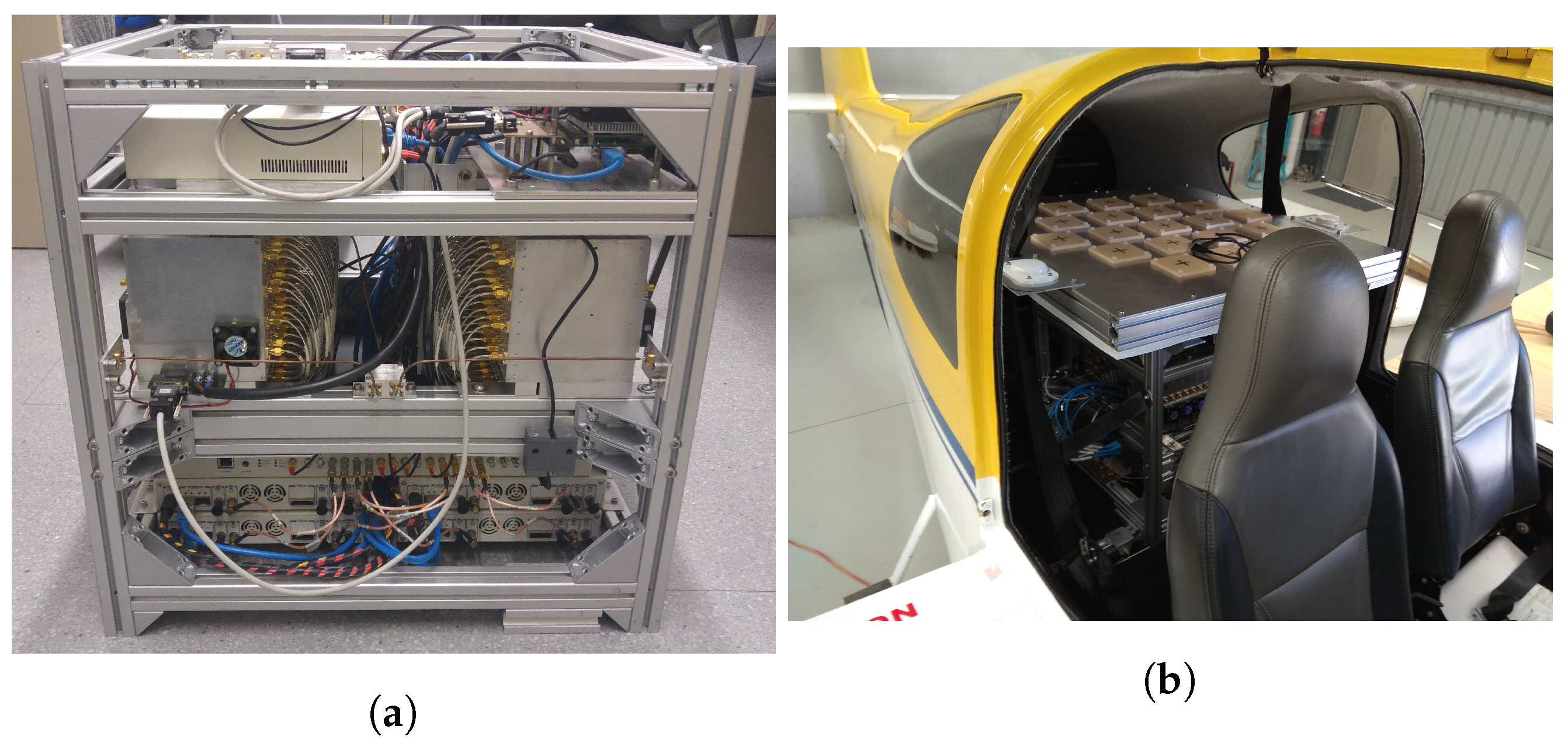
2.1. Receiver Specifications
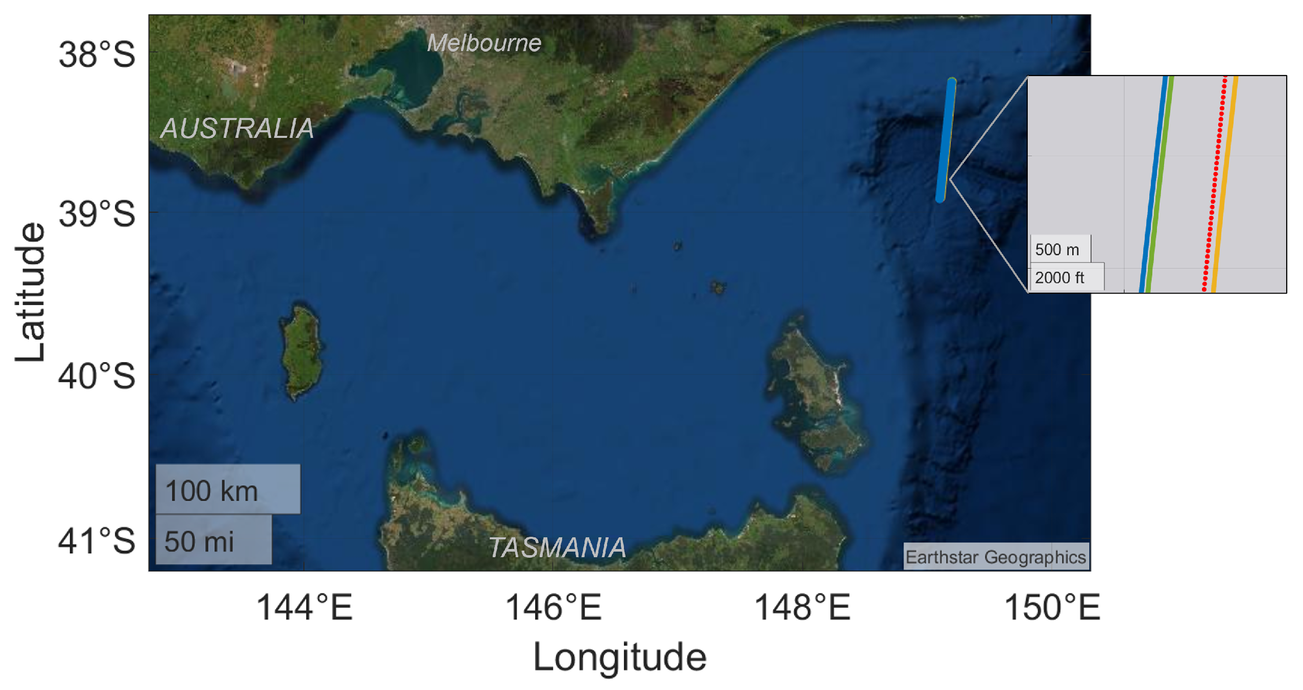
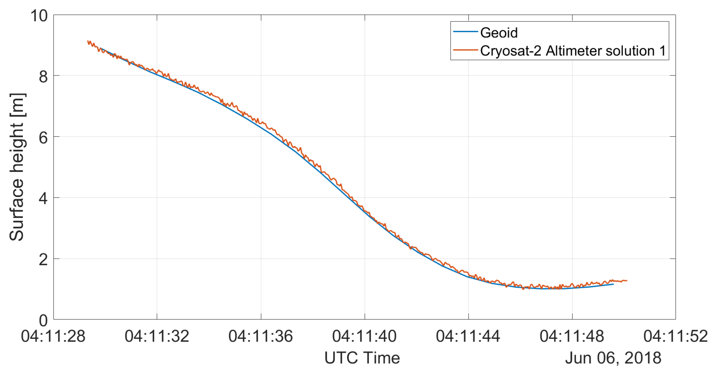
2.2. Data
3. Altimetric Methods
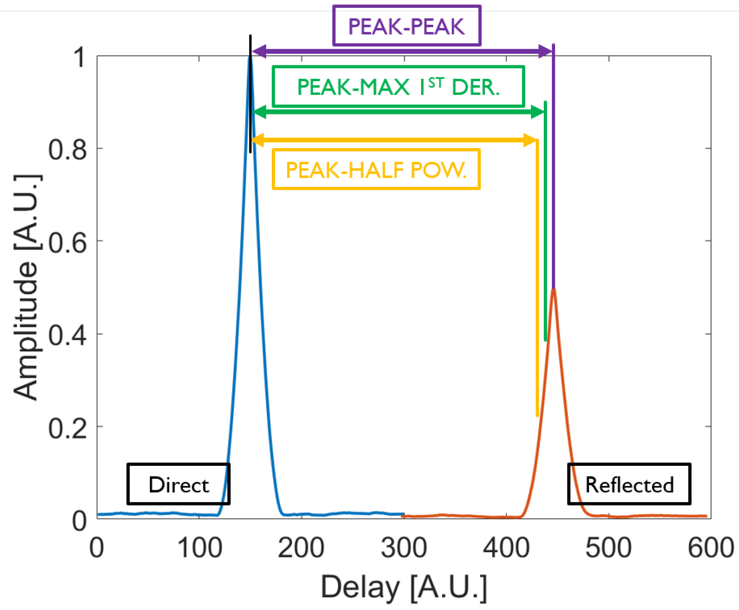
- In Peak-to-Peak (P-P), the peak (maximum) of the waveform is optimal for the direct signal. However, for the reflected case, it will only be optimal if the reflection is specular. As seen in [54], during the analyzed flight the wind-driven waves were ∼1.7 m high with a period of 5 s, and the swell waves were ∼1.2 m high with a period of 10 s. Therefore, the flat surface condition (Rayleigh criterion, Equation (7), [35,59]) is not satisfied for the frequencies and incidence angles considered, and the reflection was not specular.
- The second method considered uses the peak of the direct signal waveform, and the maximum of the first derivative of the reflected signal waveform (P-Max1D) [49].
- The third method tracks the Half-power position of the waveform (P-HP), as in radar altimetry [60]. It is adapted to GNSS-R using the peak of the direct signal waveform and the half-power point of the leading-edge of the reflected signal waveform. The main difference with respect to radar altimetry is that the bandwidths used in GNSS-R are much smaller, at least by an order of magnitude. Based on the model of the position of the maximum of the first derivative [49], some GNSS-R experiments [21,41] have also used this technique, but using the point at 70% instead.
- Finally, to overcome the limitations of the previous methods, a new method is proposed: the use of the peak of the direct signal waveforms and the minimum of the 3rd derivative of the reflected signal waveform (P-Min3D).
3.1. GNSS-R Altimetry Using the Peak-to-Minimum of the 3rd Derivative
3.1.1. Case 1
3.1.2. Case 2
4. Results
4.1. Altimetric Methods
- In the first part of the table L1 cGNSS-R cases are shown.
- -
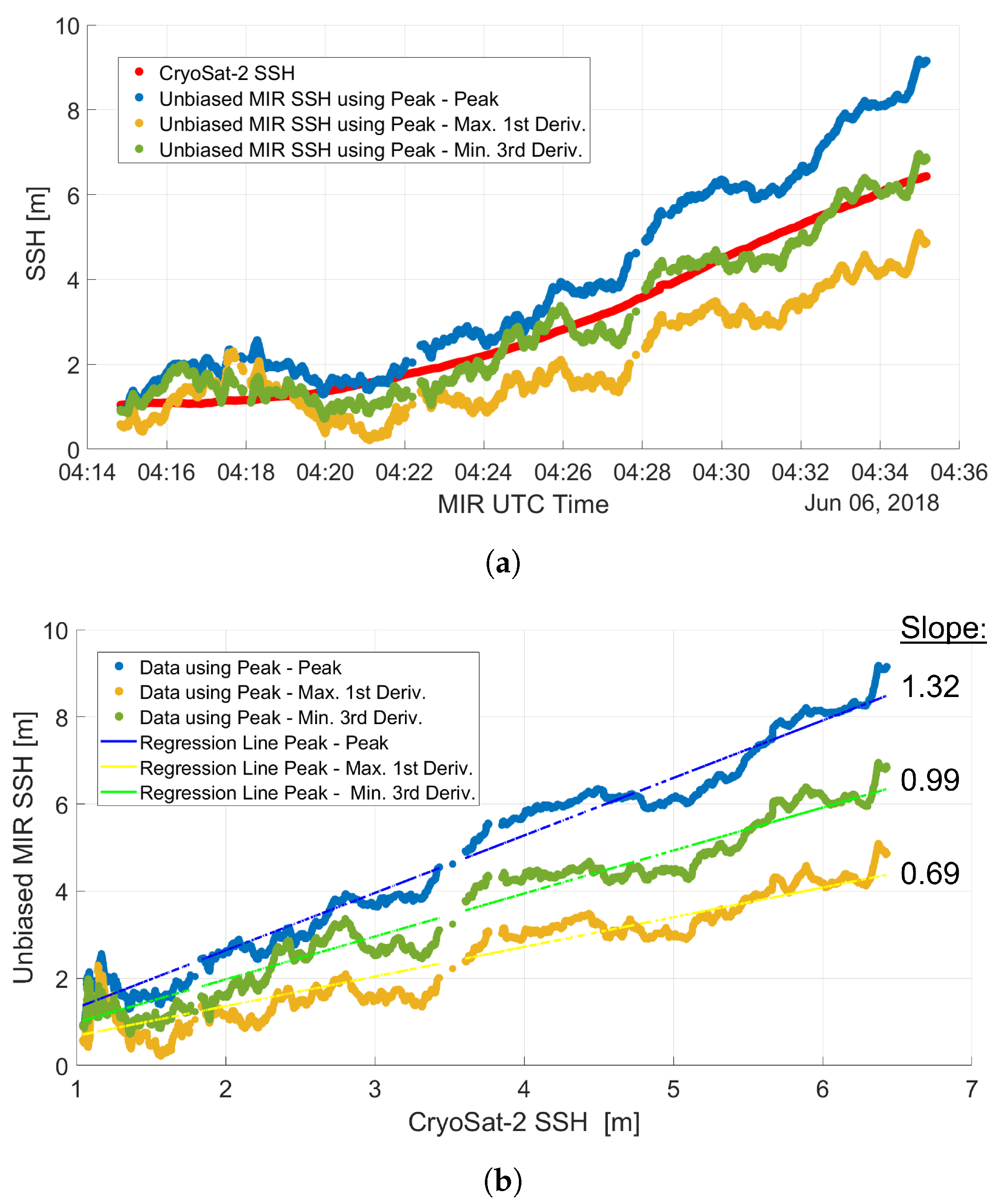
- The P-P method is not optimal as the slope is significantly larger than 1.
- -
- The P-Max1D is not optimal either. As explained in Section 3.1, results match with the simulation of P-Min3D, where, due to the finite bandwidth, the tracking position shifts.
- -
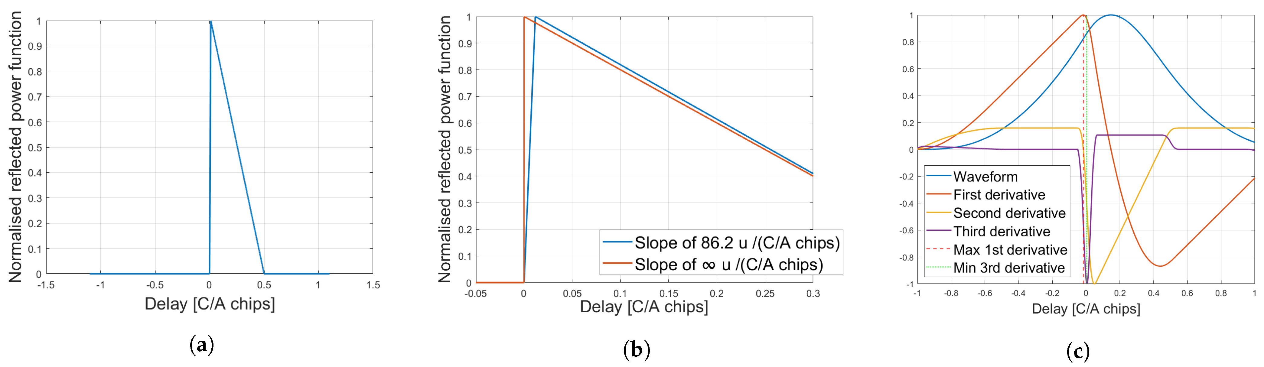
- The P-HP shows the worst results. L1 C/A signal limited bandwidth (Table 1) makes a wide waveform with a gradual leading edge. Figure 9c) shows that the 50% position is shifted almost 0.2 C/A chips (∼58 m) from the optimal zero delay, which explains the large offset and that the behaviorfrom the estimates is so far away from the optimal (slope 1). As it will be seen, this method extrapolated from radar altimetry works better with larger bandwidth signals with a steeper leading edge.
- -
- The next section of the Table 2 shows the main results for the cGNSS-R at L5:
- -
- As in L1, the P-P method does not offer the best performance. As it has been stated, this method works best with specular reflections and the sea waves present on that day induce a non-specular reflection.
- -
- The P-Max1D performs slightly better than at L1. In the L5 case, the first derivative maximum is close to the half power position (Figure 12b), because of the steepness of the waveform.
- -
- The P-HP achieves the best slope (i.e., closest to 1). L5 codes have a large bandwidth, 10 times larger than L1 C/A codes. which leads to a sharper waveform (Figure 13).
- -
- Finally, the P-Min3D presents a similar behaviorto the P-Max1D. Its position is closer to the half power position as now the leading edge is much steeper, due to the larger bandwidth.
- The slopes of the E5a waveforms have a similar behaviorto those of at L5. The waveform shapes are very similar (Figure 13b,c), and the code bandwidth is the same. The P-HP method is the one with the closest slope to 1. Galileo E5a transmitted power is also 3 dB higher than GPS L5 [10], this is likely to be the reason why, in general, all the slopes are better than at L5.
- As shown in Table 1, iGNSS-R cases exhibit a lower SNR than cGNSS-R, and lower at L1 than at L5. L1 waveforms also present multiple correlation peaks overlapping in the same composite waveform, formed by the correlation of the different signals present at L1 (e.g., C/A, P(Y) or M-codes). The low SNR, and the different shapes present in the waveforms are actually a challenge for these methods. The P-P method is the one performing the best for this case. It usually tracked the peak of the correlation of the encrypted codes, although not in the optimal position for non-specular reflections. For these reasons, the slope of the fit is worse than for the other cases.
- The iGNSS-R L5 case is quite similar to the conventional case, as it is already using large bandwidth codes. The secondary peaks from secondary reflections which sometimes appear in the L5 waveforms [54] are also present. As in the L5 conventional case the P-HP achieves the slope closest to 1.
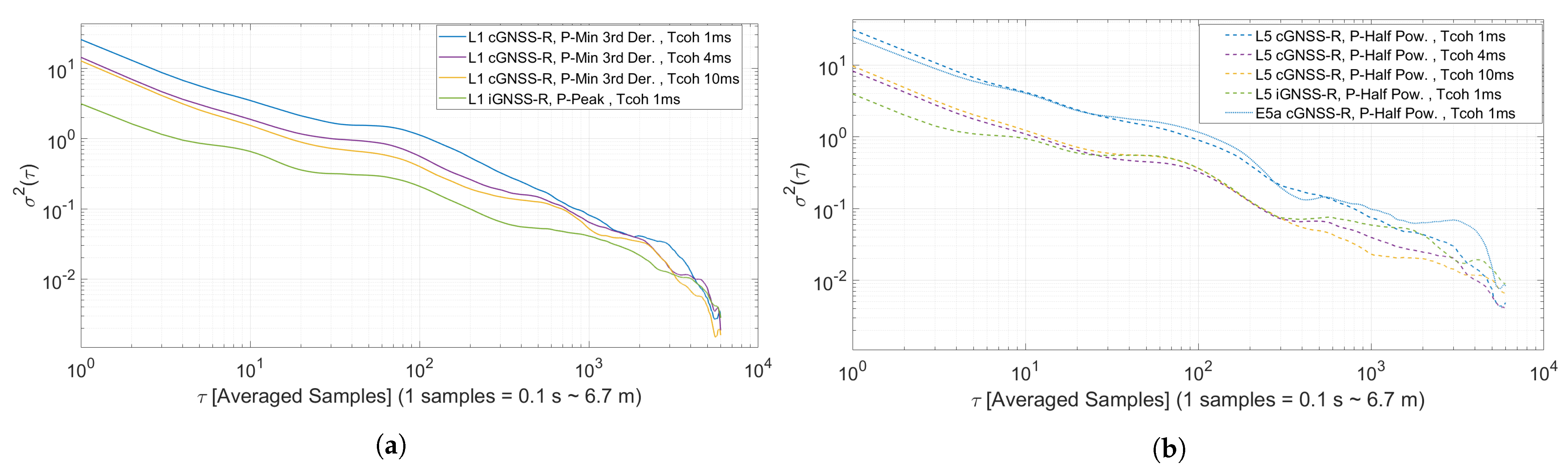
4.2. Allan Variance
- L1 cGNSS-R with ms measurements with few averaged samples have less variance than those from the L5. This might be due to the oversampling at L1. MIR uses 32 samples per C/A chip, at L5 due to the narrower waveforms the number of samples defining the peak is smaller. As the averaging increases, L5 starts to show a smaller variance than the L1 ones, although both results are quite close.
- L1 and L5 cGNSS-R at long coherent integration times, ms and ms exhibit better performance, at L5 better than L1. At L1 cGNSS-R the SNR improved with longer coherent integration times, and the variance decreased as the SNR increased. At L5, the SNR also increased with longer coherent integration times, but for ms the variance is smaller than for ms. This behavioris attributed to the coherence time of a surface () which can be estimated as Equation (8) [56].where is the wavelength; v the platform speed; h is the height; c the speed of light; is the duration of a chip; and the incidence angle. For the conditions of this flight, at L1, the coherency would be lost after 2 ms for ° or 2.8 ms for ° [63], so the improvement in 4 and 10 ms is purely linked to the SNR improvement. However, at L5 coherency would be lost after 7.7 ms for ° or 10 ms for ° [63]. Since varied from 31° to 21°, it never reached 10 ms, but the coherence of the surface was always longer than for 4 ms. This is clearly shown by the L5 variance which reached the better value for ms.
- The iGNSS-R cases achieved the smallest variances since they have largest bandwidths, despite the lower SNRs. In this particular case L1 is a bit better than L5. iGNSS-R cases are limited by the receiver’s bandwidth and the maximum bandwidths transmitted at the band. In L5 MIR bandwidth ∼34 MHz is larger than the total transmitted bandwidth at L5, 24 MHz, so noise is being added to the signal. At L1 MIR bandwidth ∼20 MHz is lower than the 30.69 MHz transmitted, in this case the maximum resolution [10] is limited by the bandwidth, but there is no addition of noise due to a larger bandwidth.
- E5a measurements (cGNSS-R with ms), start with a variance similar to L1, and as the averaging increases it shows similar variances to the L1 and L5 cGNSS-R ones with ms.
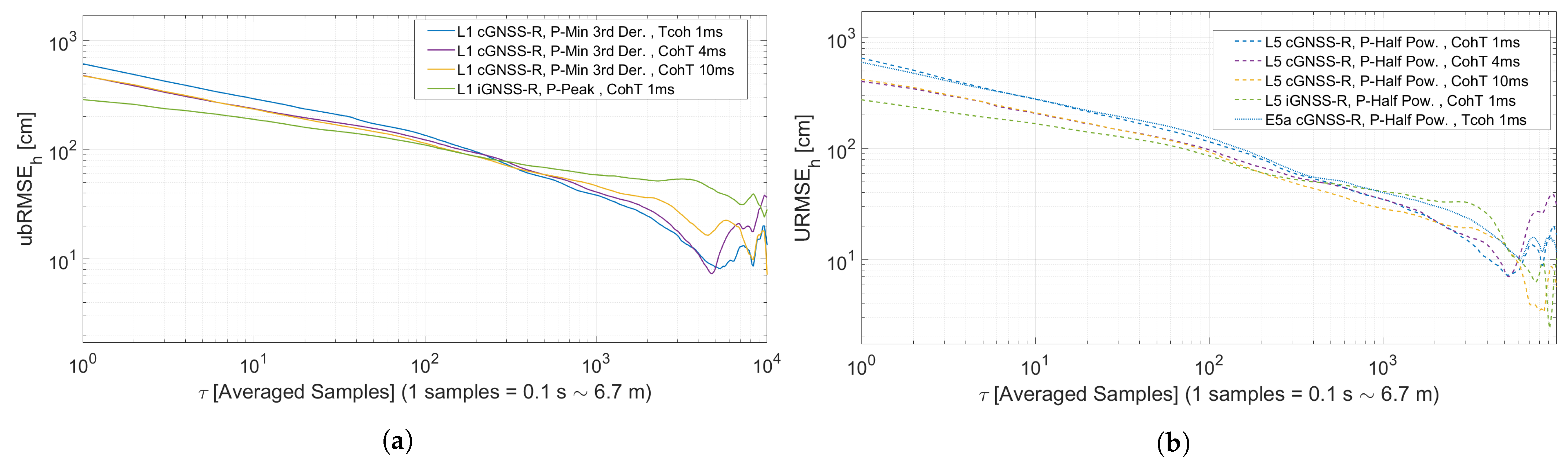
4.3. ubRMSE
5. Discussion
- iGNSS-R cases achieved the best results showing an ubRMSE improvement of a factor of ∼2.2 with respect to the same band and using the cGNSS-R technique. From the simulated precisions for GEROS-ISS [42], more improvement was predicted when using the iGNSS-R technique as compared to the cGNSS-R technique. However, this was a space-borne prediction, and considering dual-frequency observables, among many other corrections, which makes the results hardly comparable. Differently, it was experimentally shown [32] that the improvement factor when using P(Y) with the reconstructed GNSS-R (rGNSS-R) technique compared to C/A with the cGNSS-R technique was ∼2.4. Considering that rGNSS-R will have a higher SNR than iGNSS-R it matches that the improvement factor is higher for rGNSS-R, but with very similar magnitudes.
- Comparing L1 and L5 iGNSS-R cases, they performed similar with low averages, but L5 better overall. L5 iGNSS-R signal had almost 8 dB more SNR than L1 iGNSS-R, and MIR bandwidth is more limited at L1 than at L5. Therefore, the expected achievable resolution was lower at L1 than at L5, and the results show this behavior. Theoretical optima have been analyzed in [10], showing that L1 should perform better than L5. However, the conditions considered for the theoretical analysis are distinct than the ones provided by MIR, as in that analysis the signals are considered to have the optimal bandwidth and same 20 dB SNR, while MIR signals have different bandwidths than the theoretical optimal and SNR varies with the signal. For these reasons both iGNSS-R cases have these performances.
- A similar thing happens with the E5a signal. It does perform the best for cGNSS-R with ms and ms, but when increasing the incoherent averaging it does not have a clear advantage compared with L5. According to the GEROS-ISS simulations [42] Galileo signal should perform the best, but again it is considering dual-frequency observables. And looking at the optimal parameters again [10], the most optimal parameters are not met. Also, the signals come form different satellites which may generate significant differences for its fair comparison. Between the L1 and L5 cGNSS-R cases, L5 performs better than L1, because L1 only uses the C/A code, which has a narrower bandwidth compared to L5 code.
- Increasing the coherent integration time in cGNSS-R cases increases the SNRs, which improves the ubRMSE. An improvement of a factor of ∼1.3–1.6 is observed with respect to the ms. The best performance with coherent integration time is observed when the coherency of the surface is considered, as at L5.
6. Conclusions
Author Contributions
Funding
Institutional Review Board Statement
Informed Consent Statement
Data Availability Statement
Conflicts of Interest
Abbreviations
| MIR | Microwave Interferometric Reflectometer |
| GNSS | Global Navigation Satellite System |
| Peak-to-Minimum of the 3rd Derivative | P-Min3D |
| Peak-to-Half Power | P-HP |
| Peak-to-Peak | P-P |
| Peak-to-Maximum of the 1st Derivative | P-Max1D |
| GNSS-R | Global Navigation Satellite System Reflectometry |
| cGNSS-R | Conventional GNSS-R |
| iGNSS-R | Interferometric GNSS-R |
| rGNSS-R | Reconstructed GNSS-R |
| Bw | Bandwidth |
| Coherent integration time | |
| Incoherent integration number | |
| Incoherent integration time | |
| SNR | Signal to Noise Ratio |
| w.r.t. | With respect to |
| SSH | Sea Surface Height |
| ubRMSE | Unbiased Root Mean Squared Error |
| Min | Minimum |
| Max | Maximum |
| Der | Derivative |
| UTC | Coordinated Universal Time |
| NN | Neural Network |
References
- Martin-Neira, M. A Passive Reflectometry and Interferometry System (PARIS): Application to ocean altimetry. ESA J. 1993, 17, 331–355. [Google Scholar]
- Treuhaft, R.N.; Lowe, S.T.; Zuffada, C.; Chao, Y. 2-cm GPS altimetry over Crater Lake. Geophys. Res. Lett. 2001, 28, 4343–4346. [Google Scholar] [CrossRef]
- Martin-Neira, M.; Caparrini, M.; Font-Rossello, J.; Lannelongue, S.; Vallmitjana, C. The PARIS concept: An experimental demonstration of sea surface altimetry using GPS reflected signals. IEEE Trans. Geosci. Remote Sens. 2001, 39, 142–150. [Google Scholar] [CrossRef] [Green Version]
- Martin-Neira, M.; Colmenarejo, P.; Ruffini, G.; Serra, C. Altimetry precision of 1 cm over a pond using the wide-lane carrier phase of GPS reflected signals. Can. J. Remote Sens. 2002, 28, 394–403. [Google Scholar] [CrossRef]
- Lowe, S.T.; Zuffada, C.; Chao, Y.; Kroger, P.; Young, L.E.; LaBrecque, J.L. 5-cm-Precision aircraft ocean altimetry using GPS reflections. Geophys. Res. Lett. 2002, 29, 13-1–13-4. [Google Scholar] [CrossRef] [Green Version]
- Ruffini, G.; Soulat, F.; Caparrini, M.; Germain, O.; Martín-Neira, M. The Eddy Experiment: Accurate GNSS-R ocean altimetry from low altitude aircraft. Geophys. Res. Lett. 2004, 31. [Google Scholar] [CrossRef] [Green Version]
- Martin-Neira, M.; D’Addio, S.; Buck, C.; Floury, N.; Prieto-Cerdeira, R. The PARIS Ocean Altimeter In-Orbit Demonstrator. IEEE Trans. Geosci. Remote Sens. 2011, 49, 2209–2237. [Google Scholar] [CrossRef]
- Rius, A.; Nogués-Correig, O.; Ribó, S.; Cardellach, E.; Oliveras, S.; Valencia, E.; Park, H.; Tarongí, J.M.; Camps, A.; van der Marel, H.; et al. Altimetry with GNSS-R interferometry: First proof of concept experiment. GPS Solut. 2011, 16, 231–241. [Google Scholar] [CrossRef]
- Garrison, J.L.; Katzberg, S.J.; Hill, M.I. Effect of sea roughness on bistatically scattered range coded signals from the Global Positioning System. Geophys. Res. Lett. 1998, 25, 2257–2260. [Google Scholar] [CrossRef] [Green Version]
- Pascual, D.; Camps, A.; Martin, F.; Park, H.; Arroyo, A.A.; Onrubia, R. Precision Bounds in GNSS-R Ocean Altimetry. IEEE J. Sel. Top. Appl. Earth Obs. Remote Sens. 2014, 7, 1416–1423. [Google Scholar] [CrossRef]
- Li, W.; Cardellach, E.; Fabra, F.; Rius, A.; Ribó, S.; Martín-Neira, M. First spaceborne phase altimetry over sea ice using TechDemoSat-1 GNSS-R signals. Geophys. Res. Lett. 2017, 44, 8369–8376. [Google Scholar] [CrossRef]
- Cardellach, E.; Ao, C.O.; de la Torre Juárez, M.; Hajj, G.A. Carrier phase delay altimetry with GPS-reflection/occultation interferometry from low Earth orbiters. Geophys. Res. Lett. 2004, 31. [Google Scholar] [CrossRef]
- Fabra, F.; Cardellach, E.; Rius, A.; Ribo, S.; Oliveras, S.; Nogues-Correig, O.; Belmonte Rivas, M.; Semmling, M.; D’Addio, S. Phase Altimetry With Dual Polarization GNSS-R Over Sea Ice. IEEE Trans. Geosci. Remote Sens. 2012, 50, 2112–2121. [Google Scholar] [CrossRef]
- Lestarquit, L.; Peyrezabes, M.; Darrozes, J.; Motte, E.; Roussel, N.; Wautelet, G.; Frappart, F.; Ramillien, G.; Biancale, R.; Zribi, M. Reflectometry With an Open-Source Software GNSS Receiver: Use Case With Carrier Phase Altimetry. IEEE J. Sel. Top. Appl. Earth Obs. Remote Sens. 2016, 9, 4843–4853. [Google Scholar] [CrossRef]
- Yun, Z.; Binbin, L.; Luman, T.; Qiming, G.; Yanling, H.; Zhonghua, H. Phase Altimetry Using Reflected Signals From BeiDou GEO Satellites. IEEE Geosci. Remote Sens. Lett. 2016, 13, 1410–1414. [Google Scholar] [CrossRef]
- Kucwaj, J.C.; Reboul, S.; Stienne, G.; Choquel, J.B.; Benjelloun, M. Circular Regression Applied to GNSS-R Phase Altimetry. Remote Sens. 2017, 9, 651. [Google Scholar] [CrossRef] [Green Version]
- Liu, W.; Beckheinrich, J.; Semmling, M.; Ramatschi, M.; Vey, S.; Wickert, J.; Hobiger, T.; Haas, R. Coastal Sea-Level Measurements Based on GNSS-R Phase Altimetry: A Case Study at the Onsala Space Observatory, Sweden. IEEE Trans. Geosci. Remote Sens. 2017, 55, 5625–5636. [Google Scholar] [CrossRef]
- Bai, W.; Sun, Y.; Fu, Y.; Zhu, G.; Du, Q.; Zhang, Y.; Han, Y.; Cheng, C. GNSS-R open-loop difference phase altimetry: Results from a bridge experiment. Adv. Space Res. 2012, 50, 1150–1157. [Google Scholar] [CrossRef]
- Cardellach, E.; Li, W.; Rius, A.; Semmling, M.; Wickert, J.; Zus, F.; Ruf, C.S.; Buontempo, C. First Precise Spaceborne Sea Surface Altimetry With GNSS Reflected Signals. IEEE J. Sel. Top. Appl. Earth Obs. Remote Sens. 2020, 13, 102–112. [Google Scholar] [CrossRef]
- Hu, C.; Benson, C.; Rizos, C.; Qiao, L. Single-Pass Sub-Meter Space-Based GNSS-R Ice Altimetry: Results From TDS-1. IEEE J. Sel. Top. Appl. Earth Obs. Remote Sens. 2017, 10, 3782–3788. [Google Scholar] [CrossRef]
- Mashburn, J.; Axelrad, P.; Lowe, S.T.; Larson, K.M. Global Ocean Altimetry With GNSS Reflections From TechDemoSat-1. IEEE Trans. Geosci. Remote Sens. 2018, 56, 4088–4097. [Google Scholar] [CrossRef]
- Rius, A.; Cardellach, E.; Fabra, F.; Li, W.; Ribó, S.; Hernández-Pajares, M. Feasibility of GNSS-R Ice Sheet Altimetry in Greenland Using TDS-1. Remote Sens. 2017, 9, 742. [Google Scholar] [CrossRef] [Green Version]
- Hu, C.; Benson, C.R.; Qiao, L.; Rizos, C. The Validation of the Weight Function in the Leading-Edge-Derivative Path Delay Estimator for Space-Based GNSS-R Altimetry. IEEE Trans. Geosci. Remote Sens. 2020, 58, 6243–6254. [Google Scholar] [CrossRef]
- Li, W.; Cardellach, E.; Fabra, F.; Ribó, S.; Rius, A. Assessment of Spaceborne GNSS-R Ocean Altimetry Performance Using CYGNSS Mission Raw Data. IEEE Trans. Geosci. Remote Sens. 2020, 58, 238–250. [Google Scholar] [CrossRef]
- Zhang, Y.; Tian, L.; Meng, W.; Gu, Q.; Han, Y.; Hong, Z. Feasibility of Code-Level Altimetry Using Coastal BeiDou Reflection (BeiDou-R) Setups. IEEE J. Sel. Top. Appl. Earth Obs. Remote Sens. 2015, 8, 4130–4140. [Google Scholar] [CrossRef]
- Cartwright, J.; Banks, C.J.; Srokosz, M. Improved GNSS-R bi-static altimetry and independent digital elevation models of Greenland and Antarctica from TechDemoSat-1. Cryosphere 2020, 14, 1909–1917. [Google Scholar] [CrossRef]
- Clarizia, M.P.; Ruf, C.; Cipollini, P.; Zuffada, C. First spaceborne observation of sea surface height using GPS-Reflectometry. Geophys. Res. Lett. 2016, 43, 767–774. [Google Scholar] [CrossRef] [Green Version]
- Cardellach, E.; Rius, A.; Martín-Neira, M.; Fabra, F.; Nogués-Correig, O.; Ribó, S.; Kainulainen, J.; Camps, A.; D’Addio, S. Consolidating the Precision of Interferometric GNSS-R Ocean Altimetry Using Airborne Experimental Data. IEEE Trans. Geosci. Remote Sens. 2014, 52, 4992–5004. [Google Scholar] [CrossRef]
- Semmling, A.M.; Schmidt, T.; Wickert, J.; Schön, S.; Fabra, F.; Cardellach, E.; Rius, A. On the retrieval of the specular reflection in GNSS carrier observations for ocean altimetry. Radio Sci. 2012, 47. [Google Scholar] [CrossRef]
- Semmling, A.M.; Wickert, J.; Schön, S.; Stosius, R.; Markgraf, M.; Gerber, T.; Ge, M.; Beyerle, G. A zeppelin experiment to study airborne altimetry using specular Global Navigation Satellite System reflections. Radio Sci. 2013, 48, 427–440. [Google Scholar] [CrossRef] [Green Version]
- Carreno-Luengo, H.; Park, H.; Camps, A.; Fabra, F.; Rius, A. GNSS-R Derived Centimetric Sea Topography: An Airborne Experiment Demonstration. IEEE J. Sel. Top. Appl. Earth Obs. Remote Sens. 2013, 6, 1468–1478. [Google Scholar] [CrossRef]
- Carreno-Luengo, H.; Camps, A.; Ramos-Pérez, I.; Rius, A. Experimental Evaluation of GNSS-Reflectometry Altimetric Precision Using the P(Y) and C/A Signals. IEEE J. Sel. Top. Appl. Earth Obs. Remote Sens. 2014, 7, 1493–1500. [Google Scholar] [CrossRef]
- Ichikawa, K.; Ebinuma, T.; Konda, M.; Yufu, K. Low-Cost GNSS-R Altimetry on a UAV for Water-Level Measurements at Arbitrary Times and Locations. Sensors 2019, 19, 998. [Google Scholar] [CrossRef] [Green Version]
- Ribot, M.A.; Kucwaj, J.C.; Botteron, C.; Reboul, S.; Stienne, G.; Leclère, J.; Choquel, J.B.; Farine, P.A.; Benjelloun, M. Normalized GNSS Interference Pattern Technique for Altimetry. Sensors 2014, 14, 10234–10257. [Google Scholar] [CrossRef] [PubMed] [Green Version]
- Alonso-Arroyo, A.; Camps, A.; Park, H.; Pascual, D.; Onrubia, R.; Martín, F. Retrieval of Significant Wave Height and Mean Sea Surface Level Using the GNSS-R Interference Pattern Technique: Results From a Three-Month Field Campaign. IEEE Trans. Geosci. Remote Sens. 2015, 53, 3198–3209. [Google Scholar] [CrossRef] [Green Version]
- Geremia-Nievinski, F.; Hobiger, T.; Haas, R.; Liu, W.; Strandberg, J.; Tabibi, S.; Vey, S.; Wickert, J.; Williams, S. SNR-based GNSS reflectometry for coastal sea-level altimetry: Results from the first IAG inter-comparison campaign. J. Geod. 2020, 94, 70. [Google Scholar] [CrossRef]
- Fagundes, M.A.R.; Mendonça-Tinti, I.; Iescheck, A.L.; Akos, D.M.; Geremia-Nievinski, F. An open-source low-cost sensor for SNR-based GNSS reflectometry: Design and long-term validation towards sea-level altimetry. GPS Solut. 2021, 25, 73. [Google Scholar] [CrossRef]
- Zavorotny, V.U.; Gleason, S.; Cardellach, E.; Camps, A. Tutorial on Remote Sensing Using GNSS Bistatic Radar of Opportunity. IEEE Geosci. Remote Sens. Mag. 2014, 2, 8–45. [Google Scholar] [CrossRef] [Green Version]
- Hajj, G.A.; Zuffada, C. Theoretical description of a bistatic system for ocean altimetry using the GPS signal. Radio Sci. 2003, 38. [Google Scholar] [CrossRef]
- Gleason, S.; Gommenginger, C.; Cromwell, D. Fading statistics and sensing accuracy of ocean scattered GNSS and altimetry signals. Adv. Space Res. 2010, 46, 208–220. [Google Scholar] [CrossRef]
- Mashburn, J.; Axelrad, P.; Lowe, S.T.; Larson, K.M. An Assessment of the Precision and Accuracy of Altimetry Retrievals for a Monterey Bay GNSS-R Experiment. IEEE JOurnal Sel. Top. Appl. Earth Obs. Remote Sens. 2016, 9, 4660–4668. [Google Scholar] [CrossRef]
- Camps, A.; Park, H.; Sekulic, I.; Rius, J.M. GNSS-R Altimetry Performance Analysis for the GEROS Experiment on Board the International Space Station. Sensors 2017, 17, 1583. [Google Scholar] [CrossRef] [PubMed] [Green Version]
- Park, H.; Camps, A.; Valencia, E.; Rodriguez-Alvarez, N.; Bosch-Lluis, X.; Ramos-Perez, I.; Carreno-Luengo, H. Retracking considerations in spaceborne GNSS-R altimetry. GPS Solut. 2012, 16, 507–518. [Google Scholar] [CrossRef]
- Park, H.; Valencia, E.; Camps, A.; Rius, A.; Ribo, S.; Martin-Neira, M. Delay Tracking in Spaceborne GNSS-R Ocean Altimetry. IEEE Geosci. Remote Sens. Lett. 2013, 10, 57–61. [Google Scholar] [CrossRef]
- Martín-Neira, M.; D’Addio, S.; Vitulli, R. Study of Delay Drift in GNSS-R Altimetry. IEEE J. Sel. Top. Appl. Earth Obs. Remote Sens. 2014, 7, 1473–1480. [Google Scholar] [CrossRef]
- Ozafrain, S.; Roncagliolo, P.A.; Muravchik, C.H. Likelihood Map Waveform Tracking Performance for GNSS-R Ocean Altimetry. IEEE J. Sel. Top. Appl. Earth Obs. Remote Sens. 2019, 12, 5379–5384. [Google Scholar] [CrossRef]
- Ghavidel, A.; Schiavulli, D.; Camps, A. Numerical Computation of the Electromagnetic Bias in GNSS-R Altimetry. IEEE Trans. Geosci. Remote Sens. 2016, 54, 489–498. [Google Scholar] [CrossRef] [Green Version]
- Park, J.; Johnson, J.T.; Lowe, S.T. A study of the electromagnetic bias for GNSS-R ocean altimetry using the choppy wave model. Waves Random Complex Media 2016, 26, 599–612. [Google Scholar] [CrossRef]
- Rius, A.; Cardellach, E.; Martin-Neira, M. Altimetric Analysis of the Sea-Surface GPS-Reflected Signals. IEEE Trans. Geosci. Remote Sens. 2010, 48, 2119–2127. [Google Scholar] [CrossRef]
- Martín, F.; Camps, A.; Park, H.; D’Addio, S.; Martín-Neira, M.; Pascual, D. Cross-Correlation Waveform Analysis for Conventional and Interferometric GNSS-R Approaches. IEEE J. Sel. Top. Appl. Earth Obs. Remote Sens. 2014, 7, 1560–1572. [Google Scholar] [CrossRef]
- Pascual, D.; Park, H.; Camps, A.; Arroyo, A.A.; Onrubia, R. Simulation and Analysis of GNSS-R Composite Waveforms Using GPS and Galileo Signals. IEEE J. Sel. Top. Appl. Earth Obs. Remote Sens. 2014, 7, 1461–1468. [Google Scholar] [CrossRef]
- Onrubia, R.; Pascual, D.; Querol, J.; Park, H.; Camps, A. The Global Navigation Satellite Systems Reflectometry (GNSS-R) Microwave Interferometric Reflectometer: Hardware, Calibration, and Validation Experiments. Sensors 2019, 19, 1019. [Google Scholar] [CrossRef] [Green Version]
- ESA/ESTEC. CryoSat Mission and Data Description. 2007. Available online: http://esamultimedia.esa.int/docs/Cryosat/Mission_and_Data_Descrip.pdf (accessed on 15 May 2021).
- Munoz-Martin, J.F.; Onrubia, R.; Pascual, D.; Park, H.; Camps, A.; Rüdiger, C.; Walker, J.; Monerris, A. Experimental Evidence of Swell Signatures in Airborne L5/E5a GNSS-Reflectometry. Remote Sens. 2020, 12, 1759. [Google Scholar] [CrossRef]
- Nogues, O.C.i.; Pascual, D.; Onrubia, R.; Camps, A. Advanced GNSS-R Signals Processing With GPUs. IEEE J. Sel. Top. Appl. Earth Obs. Remote Sens. 2020, 13, 1158–1163. [Google Scholar] [CrossRef]
- Camps, A.; Park, H.; Valencia i Domènech, E.; Pascual, D.; Martin, F.; Rius, A.; Ribo, S.; Benito, J.; Andrés-Beivide, A.; Saameno, P.; et al. Optimization and Performance Analysis of Interferometric GNSS-R Altimeters: Application to the PARIS IoD Mission. IEEE J. Sel. Top. Appl. Earth Obs. Remote Sens. 2014, 7, 1436–1451. [Google Scholar] [CrossRef]
- Onrubia Ibáñez, R. Advanced GNSS-R Instruments for Altimetric and Scatterometric Applications. Ph.D. Thesis, UPC, Departament de Teoria del Senyal i Comunicacions, 2020. Available online: http://hdl.handle.net/2117/328191 (accessed on 17 October 2021).
- Camps, A.; Martín, F.; Park, H.; Valencia, E.; Rius, A.; D’Addio, S. Interferometric GNSS-R achievable altimetric performance and compression/denoising using the wavelet transform: An experimental study. In Proceedings of the 2012 IEEE International Geoscience and Remote Sensing Symposium, Munich, Germany, 22–27 July 2012; pp. 7512–7515. [Google Scholar] [CrossRef]
- Hajnsek, I.; Papathanassiou, K. Rough surface scattering models. ESA 2005. Available online: https://earth.esa.int/documents/653194/656796/Rough_Surface_Scattering_Models.pdf (accessed on 20 June 2021).
- Brown, G. The average impulse response of a rough surface and its applications. IEEE Trans. Antennas Propag. 1977, 25, 67–74. [Google Scholar] [CrossRef]
- Chelton, D.B.; Walsh, E.J.; MacArthur, J.L. Pulse Compression and Sea Level Tracking in Satellite Altimetry. J. Atmos. Ocean. Technol. 1989, 6, 407–438. [Google Scholar] [CrossRef] [Green Version]
- Allan, D.W. Historicity, strengths, and weaknesses of Allan variances and their general applications. Gyroscopy Navig. 2016, 7, 1–17. [Google Scholar] [CrossRef]
- Munoz-Martin, J.F.; Onrubia, R.; Pascual, D.; Park, H.; Camps, A.; Rüdiger, C.; Walker, J.; Monerris, A. Untangling the Incoherent and Coherent Scattering Components in GNSS-R and Novel Applications. Remote Sens. 2020, 12, 1208. [Google Scholar] [CrossRef] [Green Version]


| Sat. | Band | Available | MIR | Process. | Average SNR | |||
|---|---|---|---|---|---|---|---|---|
| PRN | BW [MHz] | beam | Tech. | [ms] | [ms] | [dB] | ||
| 3 | L1 | 2.046 | 2 | cGNSS-R | 1 | 100 | 100 | 20.5 |
| 3 | L1 | 2.046 | 2 | cGNSS-R | 4 | 25 | 100 | 26.5 |
| 3 | L1 | 2.046 | 2 | cGNSS-R | 10 | 10 | 100 | 28.7 |
| 3 | L1 | 30.69 | 2 | iGNSS-R | 1 | 100 | 100 | 10.9 |
| 3 | L5 | 20.46 | 3 | cGNSS-R | 1 | 100 | 100 | 22.6 |
| 3 | L5 | 20.46 | 3 | cGNSS-R | 4 | 25 | 100 | 25.3 |
| 3 | L5 | 20.46 | 3 | cGNSS-R | 10 | 10 | 100 | 27.5 |
| 3 | L5 | 24.00 | 3 | iGNSS-R | 1 | 100 | 100 | 18.8 |
| E08 | E5a | 20.46 | 4 | cGNSS-R | 1 | 100 | 100 | 20.8 |
| Process. Tech. | Band | Altimetry Method | Slope [m/m] | Offset [m] |
|---|---|---|---|---|
| cGNSS-R | L1 | P-P | 1.36 | −9.42 |
| L1 | P-Max1D | 0.71 | 12.25 | |
| L1 | P-HP | 0.57 | 46.52 | |
| L1 | P-Min3D | 1.03 | 2.78 | |
| cGNSS-R | L5 | P-P | 1.35 | −8.63 |
| L5 | P-Max1D | 1.12 | 1.97 | |
| L5 | P-HP | 1.03 | 3.87 | |
| L5 | P-Min3D | 1.17 | −0.97 | |
| cGNSS-R | E5a | P-P | 1.20 | −8.39 |
| E5a | P-Max1D | 1.05 | 1.52 | |
| E5a | P-HP | 1.02 | 3.04 | |
| E5a | P-Min3D | 1.07 | −0.57 | |
| iGNSS-R | L1 | P-P | 1.14 | −4.06 |
| L1 | P-Max1D | 1.17 | 1.48 | |
| L1 | P-HP | 0.50 | 11.17 | |
| L1 | P-Min3D | 1.16 | 1.01 | |
| iGNSS-R | L5 | P-P | 1.20 | −6.84 |
| L5 | P-Max1D | 1.19 | 1.73 | |
| L5 | P-HP | 1.05 | 4.09 | |
| L5 | P-Min3D | 1.16 | 0.63 |
| Process. | Band | Altimetry | Slope | [m] | [m] | [m] | |
|---|---|---|---|---|---|---|---|
| Tech. | Method | [ms] | at 0.1 s | at 1 s | at 10 s | ||
| cGNSS-R | L1 | P-Min3D | 1 | 1.03 | 6.11 | 2.92 | 1.35 |
| cGNSS-R | L1 | P-Min3D | 4 | 1.06 | 4.78 | 2.37 | 1.22 |
| cGNSS-R | L1 | P-Min3D | 10 | 0.99 | 4.74 | 2.34 | 1.14 |
| iGNSS-R | L1 | P-P | 1 | 1.14 | 2.87 | 1.89 | 1.10 |
| cGNSS-R | L5 | P-HP | 1 | 1.03 | 6.53 | 2.78 | 1.14 |
| cGNSS-R | L5 | P-HP | 4 | 1.05 | 4.03 | 2.07 | 0.97 |
| cGNSS-R | L5 | P-HP | 10 | 1.04 | 4.20 | 2.09 | 0.92 |
| iGNSS-R | L5 | P-HP | 1 | 1.05 | 2.75 | 1.67 | 0.85 |
| cGNSS-R | E5a | P-HP | 1 | 1.02 | 5.99 | 2.79 | 1.25 |
Publisher’s Note: MDPI stays neutral with regard to jurisdictional claims in published maps and institutional affiliations. |
© 2021 by the authors. Licensee MDPI, Basel, Switzerland. This article is an open access article distributed under the terms and conditions of the Creative Commons Attribution (CC BY) license (https://creativecommons.org/licenses/by/4.0/).
Share and Cite
Nogués, O.C.i.; Munoz-Martin, J.F.; Park, H.; Camps, A.; Onrubia, R.; Pascual, D.; Rüdiger, C.; Walker, J.P.; Monerris, A. Improved GNSS-R Altimetry Methods: Theory and Experimental Demonstration Using Airborne Dual Frequency Data from the Microwave Interferometric Reflectometer (MIR). Remote Sens. 2021, 13, 4186. https://0-doi-org.brum.beds.ac.uk/10.3390/rs13204186
Nogués OCi, Munoz-Martin JF, Park H, Camps A, Onrubia R, Pascual D, Rüdiger C, Walker JP, Monerris A. Improved GNSS-R Altimetry Methods: Theory and Experimental Demonstration Using Airborne Dual Frequency Data from the Microwave Interferometric Reflectometer (MIR). Remote Sensing. 2021; 13(20):4186. https://0-doi-org.brum.beds.ac.uk/10.3390/rs13204186
Chicago/Turabian StyleNogués, Oriol Cervelló i, Joan Francesc Munoz-Martin, Hyuk Park, Adriano Camps, Raul Onrubia, Daniel Pascual, Christoph Rüdiger, Jeffrey P. Walker, and Alessandra Monerris. 2021. "Improved GNSS-R Altimetry Methods: Theory and Experimental Demonstration Using Airborne Dual Frequency Data from the Microwave Interferometric Reflectometer (MIR)" Remote Sensing 13, no. 20: 4186. https://0-doi-org.brum.beds.ac.uk/10.3390/rs13204186