Article

USA Crop Yield Estimation with MODIS NDVI: Are Remotely Sensed Models Better than Simple Trend Analyses?

1
United States Department of Agriculture/National Agricultural Statistics Service, 1400 Independence Ave. SW, Washington, DC 20250, USA
2
United States Department of Agriculture/Foreign Agricultural Service, 1400 Independence Ave. SW, Washington, DC 20250, USA
3
Goddard Space Flight Center, National Aeronautics and Space Administration/Earth Sciences Division, Code 610, Greenbelt, MD 20771, USA
*
Author to whom correspondence should be addressed.
Remote Sens. 2021, 13(21), 4227; https://0-doi-org.brum.beds.ac.uk/10.3390/rs13214227
Submission received: 20 September 2021 / Revised: 8 October 2021 / Accepted: 18 October 2021 / Published: 21 October 2021
(This article belongs to the Special Issue Advances in Remote Sensing for Crop Monitoring and Yield Estimation)

Abstract

:
Crop yield forecasting is performed monthly during the growing season by the United States Department of Agriculture’s National Agricultural Statistics Service. The underpinnings are long-established probability surveys reliant on farmers’ feedback in parallel with biophysical measurements. Over the last decade though, satellite imagery from the Moderate Resolution Imaging Spectroradiometer (MODIS) has been used to corroborate the survey information. This is facilitated through the Global Inventory Modeling and Mapping Studies/Global Agricultural Monitoring system, which provides open access to pertinent real-time normalized difference vegetation index (NDVI) data. Hence, two relatively straightforward MODIS-based modeling methods are employed operationally. The first model constitutes mid-season timing based on the maximum peak NDVI value, while the second is reflective of late-season timing by integrating accumulated NDVI over a threshold value. Corn model results nationally show the peak NDVI method provides a R2 of 0.88 and a coefficient of variation (CV) of 3.5%. The accumulated method, using an optimally derived 0.58 NDVI threshold, improves the performance to 0.93 and 2.7%, respectively. Both these models outperform simple trend analysis, which is 0.48 and 7.4%, correspondingly. For soybeans the R2 results of the peak NDVI model are 0.62, and 0.73 for the accumulated using a 0.56 threshold. CVs are 6.8% and 5.7%, respectively. Spring wheat’s R2 performance with the accumulated NDVI model is 0.60 but just 0.40 with peak NDVI. The soybean and spring wheat models perform similarly to trend analysis. Winter wheat and upland cotton show poor model performance, regardless of method. Ultimately, corn yield forecasting derived from MODIS imagery is robust, and there are circumstances when forecasts for soybeans and spring wheat have merit too.

1. Introduction

Timely and accurate crop yield forecasting at regional and national levels is a fundamental agricultural statistic providing early insight into season-ending production totals [1]. This information helps decision-makers reduce food allocation risk through understanding the supply situation across geographies in near real-time. It serves not only as an early warning for resource apportionment but also can help guide domestic and international trade, economic and environmental policy, and highlight chronically underperforming farming areas [2,3,4].
The monitoring of crop yields over large regions can be undertaken in several ways. The traditional method is mostly through on-the-ground probability-based surveys. These usually involve contacting a random selection of farmers and asking for their opinions on their prospective yields. Alternatively, the information can also be directly obtained via biophysical measurements of the plants themselves, also through a sampling process. The United States Department of Agriculture (USDA), National Agricultural Statistics Service (NASS) has a long history of undertaking both methodologies [5], which combined inform its monthly crop production reports [6] for the United States of America (USA). Of note, the USDA more broadly monitors and tracks crop production globally through a variety of methods [7,8].
Crop yield forecasting and estimation can also be modeled. There is a lot of research toward this goal, and it is generally divided into two approaches. The first is through employing process-based models. Here all the underlying biophysical mechanisms that drive crop growth and grain production must be understood and assimilated. Input variables can include soil type, rainfall, sunlight, seed variety, plant date, fertilizer, etc. The most common process-based yield models are known by their acronyms of WOFOST [9], DSSAT [10], and APSIM [11]. Some of these models also integrate remotely sensed satellite information such as soil moisture or leaf area index [12,13,14,15]. A strong research bias has been toward modeled corn yields versus other crops with any of these methods [16,17,18,19,20]. Predictions from any of these models can be good, but they suffer from complexity in an operational setting because many input datasets and assumptions must be managed.
The second category of models is empirical. Here, observations from the past are used to inform what is happening in the present, without a strong need for understanding of the causality. The relationships between the predictor variables and the outcomes have traditionally been explored through statistical inference, but machine learning approaches can be used too. A fundamental requirement for the empirical approach is access to reliable and deep historical yield statistics, thus limiting where it can be employed, geographically. However, some governmental operational examples by organizations do exist in North America and Europe [21,22] as well as more broadly in an international context [23]. For several years, NASS has developed empirical, regional yield models for corn and soybeans in parallel with its traditional field surveys.
Imagery data from earth observation satellites have been particularly common as inputs for empirical crop yield modeling and have a long history of use. The data’s wide area coverage, timeliness, and relatively simple handling needs are all major benefits for implementation as predictor variables. Most pervasive is the use of the visible red and near-infrared (NIR) spectral bands, which have strong negative and positive correlations, respectively, with plant productivity [24,25,26,27]. Furthermore, data reduction of these two bands through the equation known as the normalized difference vegetation index (NDVI) is strongly correlated with photosynthetic capacity, and thus yield. It is calculated as:
NDVI = (NIR − red)/(NIR + red)
NDVI amplifies the contrast between the two spectral bands and has widespread adoption for use within the vegetation monitoring community. Values are unitless and can theoretically range from −1.0 to 1.0. Observations that are less than 0.3 are areas mostly devoid of vegetation, while extremely verdant spots can reach 0.9 or higher. Many other spectral band combinations exist and are used for vegetation monitoring, but NDVI performance usually competes with if not outperforms others [28], which explains its continued popularity.
The launch of the series of Advanced Very High-Resolution Radiometer (AVHRR) instruments aboard National Oceanic and Atmospheric Administration polar orbiting satellites in the early 1980 s provided the first widespread means for collecting NDVI imagery [29] for use in empirical style crop yield modeling estimation [30,31,32,33,34]. Two NDVI products were available from the AVHRR: Local Area Coverage (LAC) at 1 km spatial resolution; and Global Area Coverage (GAC) at 8 km. Though coarser, GAC data became the standard for vegetation monitoring and crop yield [35,36] given its daily global coverage as LAC data were often incomplete given the limited onboard data storage capacity of the satellites at the time. The most practical use of the imagery was shown to be creation of composited mosaics that combine the best-of, cloud free imagery over multi-day periods such as a week or a dekad [37]. This produced imagery that is ready-to-use with lower image preprocessing capacity needed by end users.
The turn of the century brought a new era of crop yield modeling with the launch of the Terra and Aqua satellites carrying the Moderate Resolution Imaging Spectroradiometer (MODIS) instrument. MODIS offered significantly better spatial resolution than AVHRR by going from at best 1 km down to 250 m. As a result, crop yield modeling efforts began shifting to leverage the data improvement provided by MODIS [38,39]. However, widespread uptake was slow due to increased data volumes, absence of a dedicated operational data delivery for agriculture, and the deep AVHRR data history. Thus, yield research with AVHRR continued [40,41,42,43,44,45]. Over time though, a history of MODIS data has accrued, leading to intensified research efforts to develop MODIS-based yield models [46,47,48,49,50,51,52].
Attempts to fully summarize the many remote-sensing-based yield modeling efforts, from both AVHRR and MODIS, have been undertaken [53,54,55]. Corn and the symbiotic crop soybeans have seen the majority of crop-specific modeling attention with MODIS [56,57,58], as has the commodity of wheat [46,59,60]. Study areas of interest have occurred throughout the world, but studies have tended to target the major grain producing areas. Efforts to combine process and empirical models have also been undertaken [61]. A shift from more traditional statistical modeling techniques to machine learning is just getting underway [62,63,64].
Yield model results from the myriad of past research, built from simple linear models using NDVI or something more sophisticated, typically range from 0.70 to 0.90 as expressed by the coefficient of determination (R2). The coefficient of variation (CV) ranges from roughly 5.0% to 20.0%. These numbers imply good performance but fail to recognize that an educated guess via simple averaging or trend modeling can often be better. This may be the reason for the lack of widespread yield modeling uptake in the applied setting. NASS itself has not fully embraced remotely sensed yield estimation but finds utility in many situations.
As such, the objective of this manuscript is to describe the within-season crop yield forecasting ability of ready-to-use, pre-summarized MODIS NDVI data at USA national and state levels used by NASS. This was measured for the dominant USA crops of corn, soybeans, spring wheat, winter wheat, and cotton. The methods shown here are not necessarily advanced but strive to provide a pragmatic approach for use in a time-sensitive, operational setting. A broader aim is to reflect the various remotely sensed yield modeling research during the MODIS era and reinforce that simple yield estimation approaches can be the best.

2. Materials and Methods
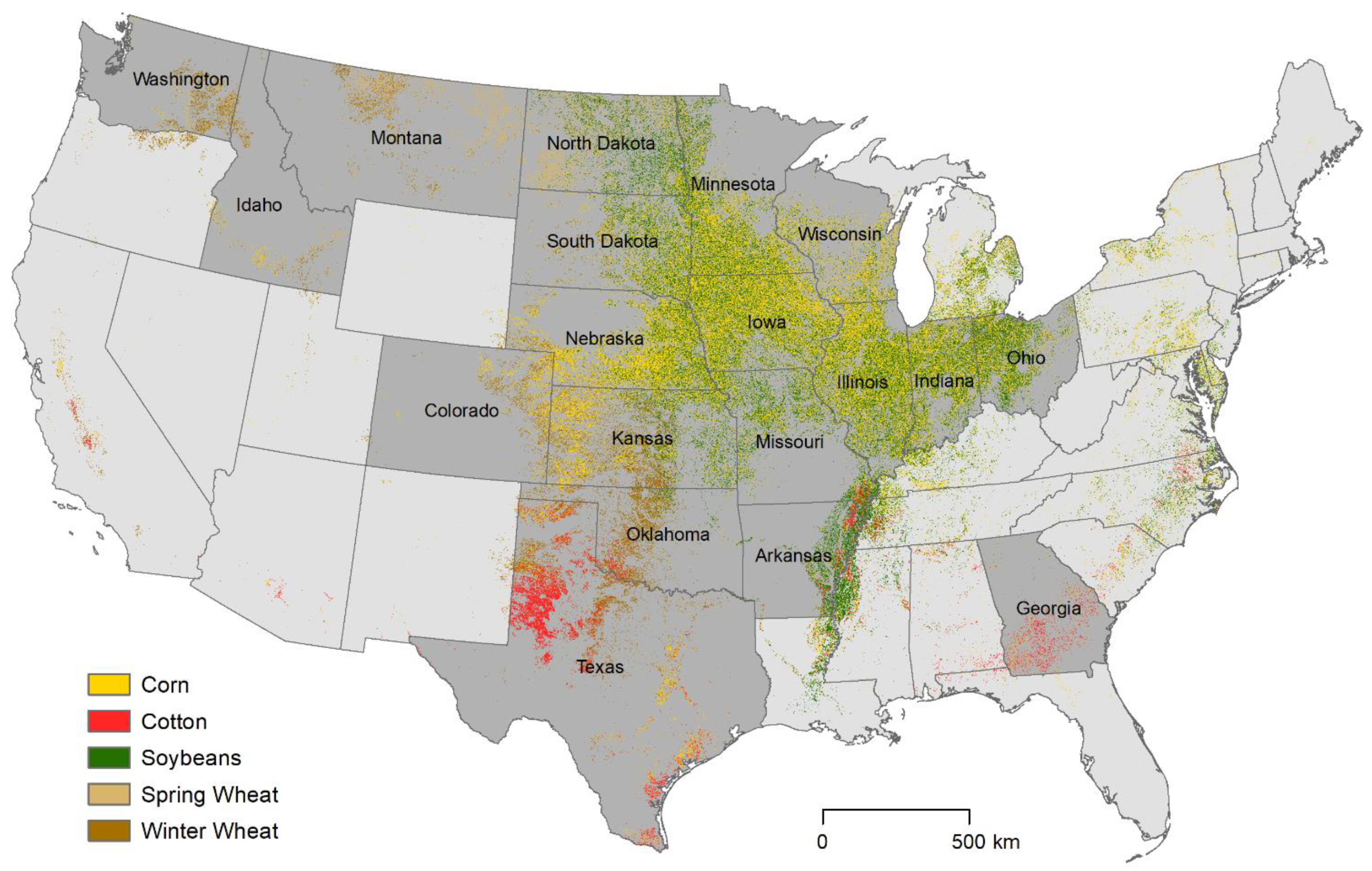
2.1. Study Area

Crops are found throughout much of the USA and are dominated by the commodities of corn, soybeans, wheat, and cotton. There are roughly 315 million acres (125 million hectares) of cropland dedicated to field crops. The past five years have averaged 91 million acres (37 million hectares) to corn, 84 million to soybeans, 12 million to spring wheat, 33 million to winter wheat, and 13 million to upland cotton [65]. This respectively equals about 29%, 27%, 4%, 11%, and 4% of the cropland total, or 75% combined.
Figure 1 shows the distribution of these primary crops across the conterminous US. Corn and soybeans are most heavily concentrated in the core of the country centered in and around the state of Iowa. This broad region is often referred to colloquially as the Corn Belt. Here the summers are warm and humid and the winters cold and snowy. Crop yields within the Corn Belt are some of the best in the world given exceptionally fertile soils and usually ample precipitation of nearly a meter per year. Only areas toward the west where it becomes drier, particularly in Nebraska, need irrigation to supplement the natural rainfall.
Adjacent west of the Corn Belt, yet east of the Rocky Mountains, is the semi-arid region known as the Great Plains. Here winter wheat, which is seeded in the fall, is planted in abundance. Because it requires less water, it can still thrive with only rainfed conditions of about half a meter per year. The state of Kansas and the immediate surrounding area grow the heaviest concentration of winter wheat in the USA. However, the crop is distributed throughout other parts of the country too, particularly in the interior areas of the northwest, such as in the state of Washington as well as in areas of the eastern and southern Corn Belt. The temperatures in these areas are generally more moderate than the Corn Belt, and thus the plants can survive winter dormancy.
Spring wheat, which is seeded in the spring, is most commonly found within the northern reaches of the Corn Belt and along the USA–Canada border. North Dakota and the surrounding states are where spring wheat is the most heavily concentrated. The region gets moderate rainfall of about half a meter per year but is extremely cold in the winter.
Finally cotton, the upland variety, is grown in the very humid south and southeast USA with pockets centered in the states of Georgia and Western Texas. Georgia receives more than a meter per year of precipitation, so irrigation is rare. Cotton in West Texas, however, is heavily dependent on irrigation given the summers are very hot and rainfall is roughly one third of Georgia’s.

2.2. Data

The foundational dataset for this work is summarized time series NDVI data provided via the Global Agriculture Monitoring (GLAM) system [66]. GLAM is operated and maintained by the Global Inventory Modeling and Mapping Studies (GIMMS) team located at the National Aeronautics and Space Administration (NASA) Goddard Space Flight Center (GSFC). The GIMMS group ensures that GLAM receives the best science quality data for NDVI production from NASA’s Land, Atmosphere Near real-time Capability for Earth Observing System (LANCE) operated by the Earth Science Data and Information System. The USDA/NASA GLAM system has been funded through an interagency agreement since 2003 by the USDA Foreign Agricultural Service (FAS), International Production Assessment Division (IPAD). This was a follow-on agreement to global AVHHR NDVI processing, which started in 2000.
The GLAM MODIS NDVI system was built from the GIMMS experience gained when providing the first operational and global AVHRR time series dataset from 1981 as referenced in the Introduction section. GIMMS developed the maximum value compositing (MVC) technique for AVHRR NDVI processing, and MVC became the standard operational cloud screening method for reducing clouds in NDVI time series composites [37]. Furthermore, the MODIS NDVI compositing algorithms were refined by the MODIS science team, which utilized a bi-directional reflectance distribution function model that includes an operational view angle constraint [67,68]. The GLAM system produces and archives eight-day NDVI imagery composites from Terra and Aqua MODIS with 250-m spatial resolution globally. Near real-time eight-day MODIS NDVI composites from LANCE are first generated. Then those are ultimately replaced a few days later with science-quality Collection 6 MOD09 NDVI composites as provided by the MODIS Adaptive Processing System as part of NASA’s Terrestrial Information Systems Branch. The data are versioned through Collections and are updated every several years to take advantage of improved processing algorithms.
GLAM also summarized the imagery to produce eight-day NDVI averages, and departure from the long-term historical averages, over national, sub-national, and 0.25-degree grid levels. These are disseminated in tabular form and eliminate the need for any image processing by an analyst. Furthermore, these averages can be tailored to exclude, or “mask”, non-agricultural areas within an area of interest. This focuses the time series signal to remove non-pertinent areas such as water bodies, urban areas, forests, etc. For the US, crop-specific masks were developed using the NASS Cropland Data Layer (CDL) [69].
The generation of these USA masks involved gathering the six years of 30 m CDLs from 2011–2016, “stacking” them, and counting for each pixel the number of occurrences by crop type during the period. Ideally, these would have been calculated over the full MODIS period, but the CDLs only exist nationally from 2008 onward, so the 2011–2016 period was used to represent the center of the time span. Next, if a 30 m CDL-scaled pixel had a specific crop two or more times during the six-year period it was flagged. The surface area of those flagged pixels was then calculated within the constraints of each 250 m MODIS pixel. If the area of the flagged 30 m pixels comprised 50 percent or more of the 250 m one, then the whole pixel was placed into the crop mask. The constraints chosen were purposely conservative to help generate the most dynamic signal. Ultimately, the full time series of NDVI data were extracted back to 2002 from GLAM using the crop-specific masks at the national and various state levels. Only the data from the MODIS morning overpass Terra were used. Note that the Terra MODIS data span back to 2000, but the first two years had time-series gaps and thus were excluded from the analyses.
In parallel, historical yield data were obtained via NASS’s Quickstats database query tool [65]. Quickstats is the consolidated repository for all NASS published data. The yield information within it comes from the annual Crop Summary [6] reports that are released every January. The Crop Summary reports document the final production, in terms of harvested area and yield, and estimates of all major USA field crops. Data were obtained over the 2002–2020 period for the nation and select states for corn, soybeans, spring and winter wheat, and upland cotton. The NASS yield data are considered the “gold standard” globally, although uncertainties are not provided. The annual yield estimates were ultimately aligned with the corresponding average MODIS NDVI data.

2.3. Methods

Three linear modeling methods were examined and performed identically by crop type. Models were fit at the USA national level and at the state level where the crop is prevalent. The predictor variable for the first model was simply year; that is, a trend model based on time was fit. The second model involved taking the annual peak, or maximum, average NDVI over the area of interest and relating that to historical yields from the same region. The third model utilized an accumulation of NDVI over the growing season and then relating that to yields. The construction of each method is explained in more detail in the following subsections.

2.3.1. Year Trend

Nineteen years of NASS yield averages were regressed against the corresponding years 2002–2020 to generate the linear trend model. In other words, the year was the independent variable and the yield the dependent variable. This could have been extended to include years prior to 2002, but to make a direct assessment against the MODIS NDVI data it was limited to 19 years. The resulting trend model could be considered the naïve guess and an easy-to-build benchmark.

2.3.2. Peak NDVI

For 2002–2020 the maximum, or peak, MODIS NDVI was obtained annually from the time series, and each year’s yield was linearly regressed against the maximum NDVI of the corresponding year. Note that the maximum NDVI did not pertain to a singular date during the growing season but rather varied in time based on the crop and unique growing conditions, as expressed with the NDVI temporal profile of that year. For winter wheat the peak NDVI tended to occur in late April, spring wheat late June, corn late July, soybeans early August, and upland cotton in the middle of August.
Figure 2 shows, for context, the NDVI time series profiles for corn over the USA for the four most extreme scenarios occurring during the period 2002–2020. Year 2018 had the earliest NDVI onset of vegetative growth, while 2019 had the latest. Year 2012 had the weakest NDVI amplitude, while 2020 was the strongest. The maximum NDVI in 2020 peaked at 0.86 but was only 0.78 in 2012, which occurred in early August and mid-July, respectively. The 2019 maximum was 0.84 and did not occur until mid-August. Of note, the corresponding published yields for years 2012, 2018, 2019, and 2020 were 123.1, 176.4, 167.5, and 172.0 bushels/acre (7.73, 11.07, 10.51, and 10.80 metric tons/hectare), respectively. The 123.1 and 176.4 values reflect the yield range for the entire period. The year 2012 was characterized by the most severe drought over the last 30 years. Year 2019 was the latest planting on record given an extremely cool and wet spring. Years 2018 and 2020 both had strong yields despite very different NDVI timings.

2.3.3. Accumulated NDVI

For 2002–2020 the accumulated, or integrated, NDVI was calculated over each growing season and then regressed against the corresponding crop yield. This seasonal integration of NDVI can be calculated in different ways, but here a method analogous to the calculation of growing degree days (GDD) [70] was employed. GDD accumulate growing season temperature over a set base, usually 10 degrees C, to produce a measure of total heating over time. Here MODIS NDVI was used instead of temperature. However, NDVI does not have a known optimal base to use as a floor for accumulating values above. If the base is set too low, there is risk of incorporating noisy or confusing NDVI information far from the mid-season peak vegetative and reproductive periods. If it is set too high, information could be lost during the vegetative green-up and brown-down periods, or the threshold might never be reached at all.
To discover an optimal NDVI threshold for the accumulation method, an iterative test was set up to understand the model performance. The coefficient of determination (R2) was used as the metric for model performance and tracked as the NDVI threshold was varied. This was conducted at the national level for all five crops. Figure 3 summarized the results graphically with the x-axis depicting the NDVI threshold value and the y-axis the model performance.
The corn yield model performance was quite insensitive to the threshold. When set between 0.45 and 0.75, the R2 was consistently above 0.90. This is reassuring and suggests there is flexibility in choosing the value. Ultimately, the corn model performed the very best when the NDVI threshold was set to 0.58, which resulted in an R2 of 0.93, so that was used as the threshold. Soybeans also showed a mostly flat response to the threshold values, although it was lower overall. The performance decreased when below 0.50. Its most optimized performance was at an NDVI of 0.56, for which the R2 was 0.73. Spring wheat had a more complicated optimal NDVI thresholding result. It was nearly flat, staying between an R2 of 0.5 and 0.6 but showed the best threshold performance at a questionably low 0.30. This was the predetermined point at which the experiment stopped given the assumption that anything much lower is background noise or irrelevant. This minimum 0.30 was kept as the spring wheat NDVI threshold, however. For winter wheat, a clear threshold optimization point occurred at 0.34, albeit the model was weak with an R2 of only 0.21. Finally, upland cotton was very poor across its possible thresholding range. It did maximize with an R2 of 0.09 at 0.37 NDVI, so that was used as a threshold. These thresholds were established at the national level and held the same for the crops during the state-level yield analysis even though tuning could improve model performance in some cases.

3. Results

USA national-level yield linear modeling depictions for the different crop types and independent variables (year, seasonal peak NDVI, and season accumulated NDVI) are shown in Figure 4. Each scatterplot has 19 points representing a year between 2002–2020. The y-axis in each is the NASS published yield average in USA units (i.e., bushels per acre or, for cotton, bales per acre). The charts in the left column contain the yield values through the years and document any temporal trend. The middle column is the annual yield versus the seasonal peak, or maximum, NDVI. The right column is the annual yield versus seasonally accumulated NDVI, over an optimized threshold. Again, for corn, soybeans, spring wheat, winter wheat, and cotton, the respective NDVI thresholds were optimized at 0.58, 0.56, 0.30, 0.34, and 0.37. The resulting least-squares regression (LSR), used for quantitative comparison, is shown as a dotted red line.
The correlation coefficient (R2), standard error (SE), and normalized SE via the coefficient of variation (CV) from each LSR are summarized in Table 1. R2 provides a comparative indication of the model performance with larger values being better. The SE and CV provide the absolute and relative model error, akin to the standard deviation. Lower error values are better. The table provides model summaries at the USA national level, as well as at the state level for select states for which the crops of interest are commonly found.
National-level yields are increasing on average through time for all crops as shown on the left column of scatterplots in Figure 4. The R2 results in Table 1 are best for soybeans at 0.72 and worst for cotton at 0.24. Corn, spring wheat, and winter wheat fall in between with R2 of 0.48, 0.58, 0.48, respectively. The strength of soybeans is notable, given it contained a low outlier year in 2012. In summary, simple linear modeling based solely on knowing the year provides some predictive insight for all crops examined but is strongest for soybeans.
The modeling using seasonal maximum peak NDVI shows mixed results. For corn the R2 is 0.88, a significant improvement from the 0.48 trend model. In terms of SE, the value drops roughly in half going from 11.4 to 5.6 bu/ac (0.72 to 0.35 mt/ha). Likewise, the CVs dropped from 7.4% to 3.5%. For the other four crops, the peak NDVI methodology performs worse than the trend. Soybeans R2 fell from 0.72 to 0.62 with the SE increasing from 2.6 to 3.0 bu/ac (0.17 to 0.20 mt/ha). Thus, CVs increased from 5.8% to 6.8%. Spring wheat showed some forecasting utility using peak NDVI by having an R2 of 0.40, but, in context, that was down from the 0.58 trend model. Winter wheat and cotton R2 results were near zero, or very poor, using peak NDVI as a yield predictor.
Results based on the accumulated NDVI method showed continued mixed results by crop. Corn nationally saw the very best model performance improving to 0.93 in terms of R2. The SE was 4.3 bu/ac (0.27 mt/ha) and thus a CV of only 2.7%. For soybeans and spring wheat the accumulated NDVI method was marginally better than using trend alone, up 0.01 to 0.73, and 0.02 to 0.60, respectively. For winter wheat and cotton the performance was worse than with trend and quite poor overall, reaching R2 values of only 0.21 and 0.09. CVs for the non-corn crops ranged from 5.7% to 8.6%, which were like those from the trend models.
Crop yield model results compared at the state level mostly mirrored those of the nation for corn and soybeans. For corn the accumulated NDVI approach was best in all cases except Ohio and Wisconsin, where the peak NDVI method was shown to be best. For all methods, the state-level averages were not as strong as the results nationally, nor was one singularly better. For soybeans, the accumulated NDVI method was the best modeling method for six of the eleven states presented. The method based simply on annual trend was best in Arkansas, Illinois, and South Dakota. The peak NDVI modeling for soybeans was best in a single state, Ohio.
In contrast though, state models for the other three crops exhibited little consistency with the national ones. Winter wheat showed the accumulated NDVI method was best in four out of six states. Spring wheat showed mixed and mostly weak performance for all states tested. Cotton was poor regardless of state or method.

4. Discussion

The efficacy of using MODIS NDVI data for USA-wide yield modeling was varied. For corn, both the mid-season peak and the season ending accumulation methodologies performed very well to excellent and easily outperformed trend analysis alone. This was nearly consistent at the state level as well providing even more confidence in the results. Corn yield estimation from MODIS data has a history of success [38,52,56,57,58] and the results here only reinforce if not improve upon it, particularly given the simplicity of the effort involved.
The modeling results for soybeans and spring wheat were also good and strengthen prior research [47,50,59,62]. This is only at first glance, however. When taken in the context of trend modeling, the results are arguably only fair. Reasons for the weakness compared to corn are unknown, but the speculation is the relationship of the soybean and spring wheat grain yields to the verdancy of the biomass, as expressed through NDVI, is simply not as strong. There is still some suggestion that the accumulated NDVI is still useful, particularly for soybeans at the state level. A better forecasting approach might be to combine the year trend and the accumulated MODIS information together in an integrated model. Alternative, MODIS information could only be relied upon when an anomaly is suggested from ancillary sources such as weather or field reports.
The results for winter wheat did not show much usefulness in any situation. This contradicts other MODIS yield research [15,46,60], but it is speculated those efforts were tested under more optimal conditions and over a shorter history. Confounding factors could be winter wheat’s much earlier growing season making it more frost prone than most crops. Furthermore, winter wheat has higher propensity to go unharvested, usually due to drought, which is hard to control for using generalized crop masks. Cotton results were even worse. There is no MODIS-based research to support or oppose these findings. As with winter wheat, an explanation could be that large swaths of cotton can go unharvested in years when growing conditions are poor. In those regions the MODIS signal is likely being heavily influenced by areas of low NDVI values that were ultimately abandoned. Using crop production instead of yield as the dependent variable might provide better modeling outcomes.
As described in the methodology, a single threshold was optimally sought for the accumulation by crop for the national-level model. Furthermore, the threshold used at the national level was propagated to the state level, both for simplicity and because the model performance was not overly sensitive to the threshold. However, the optimal thresholding levels were found to vary by state. Using state-specific thresholds can improve results for the accumulated NDVI scenario. Corn saw the biggest impact with the 10-state average R2 increasing from 0.76 to 0.81 (no table shown) and the CV decreasing from 6.5% to 5.8%. For soybeans the result was more subtle with R2 only increasing from 0.57 to 0.60 and conversely the CV decreasing from to 8.9% to 8.6%. The other crops showed little difference. In short, threshold tuning the accumulated NDVI models at finer geographic scales can in some instances produce results that more closely match those of the national level.
The modeling goal is to generate a simple estimate of the regional average yield for each crop. However, the integration of the NDVI data in context with the models can provide richer information. By applying the derived yield model to all pixels within the MODIS imagery, a map can be generated to provide detailed contextual information. Figure 5 illustrates this for corn in the year 2020. In short, the derived accumulated NDVI model equation was applied against the seasons’ worth of time series GIMMS MODIS data at a 250 m pixel resolution. To isolate only the corn areas, the 2020 CDL was used as a mask. Map areas in blue and purple are those with the highest yields. Iowa and Minnesota showed the strongest yields throughout, and this is consistent with the USDA estimate of 192.0 bu/ac (12.05 mt/ha), which was the highest in the Corn Belt that year. Iowa usually competes for the best yields annually, but 2020 saw widespread dryness, and a large derecho in early August, which decreased yields across that state. The map captures this corn yield reduction centered in Iowa. That state only realized a yield of 178.0 bu/ac (11.17 mt/ha) in 2020 even though the five years prior averaged 198 bu/ac (12.43 mt/ha).
There is a recent trend toward using finer resolution data than MODIS, which can provide yield maps at the field level [71,72,73,74,75,76] and even sub-field [77,78,79]. Finer spatial granularity is certainly important in complex landscapes [80,81] where field sizes are small. There is little doubt that this spatially detailed information has utility for field-level yield monitoring and management. Whether or not this massive quantity of data would improve regional-level yield estimation is unclear though. It is obvious that the effort would be orders of magnitude more difficult given the massive data handling needs.
Finally, it must be acknowledged that the lengthier than projected two decades long MODIS era is coming to an end. MODIS has provided a highly consistent dataset through the period allowing for unprecedented regional to global monitoring of agriculture building upon what was learned from AVHRR. This 20-year history has translated into a robust application to rapidly monitor certain crops, particularly corn, from afar. As MODIS is retired, it is natural to look toward alternative data sources, and it is anticipated the similar Visible Infrared Imaging Radiometer Suite (VIIRS) mission will be the replacement data source for this style of work. The first VIIRS instrument was placed into orbit nearly a decade ago, and a second has already followed, allowing for both historical assessment and overlap with MODIS. The uptake has been slow, likely owing to the deeper history of MODIS, the afternoon versus morning overpass time, and the spatial degradation of the red and NIR bands, which are 375 m resolution versus 250 m. Whether VIIRS will be adequate for yield modeling is yet to be tested, however.

5. Conclusions

Leveraging relatively straightforward summarized MODIS data as disseminated via the GLAM interface allows construction of an excellent corn yield model for the USA nationally. Using an accumulated NDVI method, the SE was 4.3 bu/ac (0.27 mt/ha). This equates to a CV uncertainty of only 2.7%. It seems unlikely any other modeling approach, whether empirically or physically based, could best that performance, particularly if including ease of use as a consideration. The accumulated method does have the disadvantage of needing most of the season to have transpired before being able to run, so is limited for forecasting. However, the peak NDVI method can be implemented mid-season and is still very good with SE of 5.6 bu/ac (0.35 mt/ha), or a 3.5% CV. These both significantly outperform the benchmark trend only model, which has a SE of 11.4 bu/ac (0.72 mt/ha) or a CV of 7.4%. State-level corn results are more muted but they still provide a good SE average of 9.7 bu/ac (0.61 mt/ac), equating to a CV of 6.5%, with the accumulated NDVI method. The average CVs for the peak methodology were poorer at 7.2%, but still consistently better than using a trend model, which was 10.7%.
For the other crops the usefulness of the MODIS data for yield modeling, versus simple trend, is less clear. Soybeans showed the best results at the national and state levels using the accumulated NDVI methodology, but the model estimates were only marginally better than just using trend. This is shown with the national soybean model CV, being 5.8% for trend and 5.7% for accumulated NDVI. Spring wheat also had similar CVs for both trend and accumulated NDVI, being 8.8% and 8.6%, respectively. Ultimately, the soybean and spring wheat CVs were two to three times worse than for corn. The winter wheat results were mostly poor, but there were suggestions the Northwest USA states could see some yield modeling utility with the GLAM MODIS NDVI data. All modeling scenarios for upland cotton, trend or MODIS-based, were poor. Given the success of the method for corn, it suggests for these other crops it is not so much a failure of the methodology but rather weakness in the underlying assumption of the relationship between the MODIS NDVI data and crop yield.
It is anticipated these results would be similar if the yield modeling methods were performed for intensive crop regimes globally. To concretely test this, however, is a challenge given the less comprehensive and robust historical yield estimate databases available in most countries. A secondary weakness of this modeling approach internationally is the lack of high-quality crop maps for the masking of coarse-scale imagery like MODIS. Ultimately, expansion of this style of work beyond the USA is highly welcomed, as is the pursuit of models for other crops.

Author Contributions

Conceptualization, D.M.J. and R.M.; methodology, D.M.J. and A.R.; software, D.M.J., A.R., C.R., A.A. and E.P.; validation, D.M.J., A.R. and R.M.; formal analysis, D.M.J. and A.R.; investigation, D.M.J., A.R. and R.M.; resources, R.M., R.F. and C.R.; data curation, A.A., E.P. and C.T.; writing—original draft preparation, D.M.J. and A.R.; writing—review and editing, D.M.J., A.R., R.M., C.R. and A.A., visualization, D.M.J. and C.R.; supervision, R.M., R.F. and C.T. All authors have read and agreed to the published version of the manuscript.

Funding

This research received no external funding.

Institutional Review Board Statement

Not applicable.

Informed Consent Statement

Not applicable.

Data Availability Statement

Not applicable.

Acknowledgments

This research was supported by the intramural research program of the USDA NASS Research and Development Division. The findings and conclusions in this publication have not been formally disseminated by the USDA and should not be construed to represent any agency determination or policy. Internal thanks to Eileen O’Brien, Linda Young, and Joseph Parsons for comments. External thanks to peer-reviewers’ feedback and suggestion. Special thanks to the USDA FAS IPAD for long-term interagency support to the NASA GSFC’s GIMMS group providing MODIS NDVI data processing through the GLAM system as found at https://glam1.gsfc.nasa.gov/, accessed on 18 October 2021. Finally, acknowledgement to the late Paul Doraiswamy who led the initial investigation of MODIS data toward crop yield estimation for NASS.

Conflicts of Interest

The authors declare no conflict of interest.

References

  1. World Bank. Global Strategy to Improve Agricultural and Rural Statistics; Report Number 56719-GLB; World Bank: Washington, DC, USA, 2011; Available online: http://www.fao.org/3/am082e/am082e00.pdf (accessed on 9 March 2021).
  2. Rosegrant, M.W.; Cline, S.A. Global food security: Challenges and policies. Science 2003, 302, 1917–1919. [Google Scholar] [CrossRef] [Green Version]
  3. Lobell, D.B.; Cassman, K.G.; Field, C.B. Crop Yield Gaps: Their Importance, Magnitudes, and Causes. Annu. Rev. Environ. Resour. 2009, 34, 179–204. [Google Scholar] [CrossRef] [Green Version]
  4. Carletto, C.; Jolliffe, D.; Banerjee, R. From Tragedy to Renaissance: Improving Agricultural Data for Better Policies. J. Dev. Stud. 2015, 51, 133–148. [Google Scholar] [CrossRef]
  5. US Department of Agriculture, National Agricultural Statistics Service. The Yield Forecasting Program of NASS, SMB Staff Report Number SMB 12-01. 2012. Available online: https://www.nass.usda.gov/Education_and_Outreach/Understanding_Statistics/Yield_Forecasting_Program.pdf (accessed on 25 March 2021).
  6. US Department of Agriculture, National Agricultural Statistics Service. Crop Production, Annual Summary; USDA-NASS: Washington, DC, USA, 2020; Available online: https://usda.library.cornell.edu/concern/publications/k3569432s (accessed on 17 March 2021).
  7. Vogel, F.A.; Bange, G.A. Understanding USDA Crop Forecasts. National Agricultural Statistics Service and World Agricultural Outlook Board, Office of the Chief Economist, US Department of Agriculture. 1999. Miscellaneous Publication No. 1554. Available online: https://www.nass.usda.gov/Education_and_Outreach/Understanding_Statistics/pub1554.pdf (accessed on 25 March 2021).
  8. US Department of Agriculture, World Agricultural Outlook Board. World Agricultural Supply and Demand Estimates (WASDE) Report; USDA-NASS: Washington, DC, USA, 2021. Available online: https://www.usda.gov/oce/commodity/wasde (accessed on 21 March 2021).
  9. Van Diepen, C.A.; Wolf, J.; Van Keulen, H.; Rappoldt, C. WOFOST: A simulation model of crop production. Soil Use Manag. 1989, 5, 16–24. [Google Scholar] [CrossRef]
  10. Jones, J.W.; Hoogenboom, G.; Porter, C.H.; Boote, K.J.; Batchelor, W.D.; Hunt, L.A.; Wilkens, P.W.; Singh, U.; Gijsman, A.J.; Ritchie, J.T. The DSSAT cropping system model. Eur. J. Agron. 2003, 18, 235–265. [Google Scholar] [CrossRef]
  11. Holzworth, D.P.; Huth, N.I.; deVoil, P.G.; Zurcher, E.J.; Herrmann, N.I.; McLean, G.; Chenu, K.; van Oosterom, E.J.; Snow, V.; Murphy, C.; et al. APSIM—Evolution towards a New Generation of Agricultural Systems Simulation. Environ. Modell. Softw. 2014, 62, 327–350. [Google Scholar] [CrossRef]
  12. Lambin, E.F.; Cashman, P.; Moody, A.; Parkhurst, B.H.; Pax, M.H.; Schaaf, C.B. Agricultural production monitoring in the Sahel using remote sensing: Present possibilities and research needs. J. Environ. Manag. 1993, 38, 301–322. [Google Scholar] [CrossRef]
  13. Fang, H.; Liang, S.; Hoogenboom, G. Integration of MODIS LAI and vegetation index products with the CSM-CERES-Maize model for corn yield estimation. Int. J. Remote Sens. 2011, 32, 1039–1065. [Google Scholar] [CrossRef]
  14. Ines, A.V.M.; Das, N.N.; Hansen, J.W.; Njoku, E.G. Assimilation of remotely sensed soil moisture and vegetation with a crop simulation model for maize yield prediction. Remote Sens. Environ. 2013, 138, 149–164. [Google Scholar] [CrossRef] [Green Version]
  15. Huang, J.; Tian, L.; Liang, S.; Ma, H.; Becker-Reshef, I.; Huang, Y.; Su, W.; Zhang, X.; Zhu, D.; Wu, W. Improving winter wheat yield estimation by assimilation of the leaf area index from Landsat TM and MODIS data into the WOFOST model. Agric. For. Meteorol. 2015, 204, 106–121. [Google Scholar] [CrossRef] [Green Version]
  16. Yang, H.S.; Dobermann, A.; Lindquist, J.L.; Walters, D.T.; Arkebauer, T.J.; Cassman, K.G. Hybrid-Maize—A maize simulation model that combines two crop modeling approaches. Field Crops Res. 2004, 87, 131–154. [Google Scholar] [CrossRef] [Green Version]
  17. Jin, Z.; Zhuang, Q.; Tan, Z.; Dukes, J.S.; Zheng, B.; Melillo, J.M. Do maize models capture the impacts of heat and drought stresses on yield? Using algorithm ensembles to identify successful approaches. Glob. Chang. Biol. 2016, 22, 3112–3126. [Google Scholar] [CrossRef] [PubMed]
  18. Li, Y.; Guan, K.; Schnitkey, G.D.; DeLucia, E.; Peng, B. Excessive rainfall leads to maize yield loss of a comparable magnitude to extreme drought in the United States. Glob. Chang. Biol. 2019, 25, 2325–2337. [Google Scholar] [CrossRef] [PubMed] [Green Version]
  19. Jiang, Z.; Liu, C.; Ganapathysubramanian, B.; Hayes, D.; Sarkar, S. Predicting county-scale maize yields with publicly available data. Sci. Rep. 2020, 10, 14957. [Google Scholar] [CrossRef] [PubMed]
  20. Shahhosseini, M.; Hu, G.; Archontoulis, S.V. Forecasting corn yield with machine learning ensembles. Front. Plant Sci. 2020, 11, 1120. [Google Scholar] [CrossRef] [PubMed]
  21. Chipanshi, A.; Zhang, Y.; Kouadio, L.; Newlands, N.; Davidson, A.; Hill, H.; Warren, R.; Qian, B.; Daneshfar, B.; Bedard, F.; et al. Evaluation of the Integrated Canadian Crop Yield Forecaster (ICCYF) model for in-season prediction of crop yield across the Canadian agricultural landscape. Agric. For. Meteorol. 2015, 206, 137–150. [Google Scholar] [CrossRef] [Green Version]
  22. López-Lozano, R.; Duveiller, G.; Seguini, L.; Meroni, M.; García-Condado, S.; Hooker, J.; Leo, O.; Baruth, B. Towards regional grain yield forecasting with 1km-resolution EO biophysical products: Strengths and limitations at pan-European level. Agric. For. Meteorol. 2015, 206, 12–32. [Google Scholar] [CrossRef]
  23. Becker-Reshef, I.; Justice, C.; Sullivan, M.; Vermote, E.; Tucker, C.; Anyamba, A.; Small, J.; Pak, E.; Masuoka, E.; Schmaltz, J.; et al. Monitoring Global Croplands with Coarse Resolution Earth Observations: The Global Agriculture Monitoring (GLAM). Project. Remote Sens. 2010, 2, 1589. [Google Scholar] [CrossRef] [Green Version]
  24. Tucker, C.J.; Holben, B.N.; Elgin, J.H.; McMurtrey, J.E. Relationship of spectral data to grain yield variation. Photogramm. Eng. Remote Sens. 1980, 46, 657–666. [Google Scholar]
  25. Hatfield, J.L. Remote sensing estimators of potential and actual crop yield. Remote Sens. Environ. 1983, 13, 301–311. [Google Scholar] [CrossRef]
  26. Tucker, C.J.; Sellers, P.J. Satellite remote sensing of primary production. Int. J. Remote Sens. 1986, 7, 1395–1416. [Google Scholar] [CrossRef]
  27. Bartholome, E. Radiometric measurements and crop yield forecasting. Some observations over millet and sorghum experimental plots in Mali. Int. J. Remote Sens. 1988, 9, 1539–1552. [Google Scholar] [CrossRef]
  28. Johnson, D.M. A comprehensive assessment of the correlations between field crop yields and commonly used MODIS products. Int. J. Appl. Earth Obs. 2016, 52, 65–81. [Google Scholar] [CrossRef] [Green Version]
  29. Tucker, C.J. Red and photographic infrared linear combinations for monitoring vegetation. Remote Sens. Environ. 1979, 8, 127–150. [Google Scholar] [CrossRef] [Green Version]
  30. Rasmussen, M.S. Assessment of millet yields and production in northern Burkina Faso using integrated NDVI from the AVHRR. Int. J. Remote Sens. 1992, 13, 3431–3442. [Google Scholar] [CrossRef]
  31. Groten, S.M.E. NDVI—Crop monitoring and early yield assessment of Burkina Faso. Int. J. Remote Sens. 1993, 14, 1495–1515. [Google Scholar] [CrossRef]
  32. Quarmby, N.; Mines, M.; Hindle, T.; Silleos, N. The use of multi-temporal NDVI measurements from AVHRR data for crop yield estimation and prediction. Int. J. Remote Sens. 1993, 14, 199–210. [Google Scholar] [CrossRef]
  33. Benedetti, R.; Rossini, P. On the use of NDVI profiles as a tool for agricultural statistics: The case study of wheat yield estimate and forecast in Emilia Romagna. Remote Sens. Environ. 1993, 45, 311–326. [Google Scholar] [CrossRef]
  34. Hayes, M.J.; Decker, W.L. Using NOAA AVHRR data to estimate maize production in the United States Corn Belt. Int. J. Remote Sens. 1996, 17, 3189–3200. [Google Scholar] [CrossRef]
  35. Maselli, F.; Rembold, F. Integration of LAC and GAC NDVI data to improve vegetation monitoring in semi-arid environments. Int. J. Remote Sens. 2002, 23, 2475–2488. [Google Scholar] [CrossRef]
  36. Anyamba, A.; Tucker, C.J. Historical Perspectives on AVHRR NDVI and Vegetation Drought Monitoring. In Remote Sensing for Drought: Innovative Monitoring Approaches; CRC Press/Taylor & Francis Publishers: New York, NY, USA, 2012; pp. 32–49. [Google Scholar]
  37. Holben, B.N. Characteristics of maximum-value composite images from temporal AVHRR data. Int. J. Remote Sens. 1986, 7, 1417–1434. [Google Scholar] [CrossRef]
  38. Doraiswamy, P.C.; Sinclair, T.R.; Hollinger, S.; Akhmedov, B.; Stern, A.; Prueger, J. Application of MODIS derived parameters for regional crop yield assessment. Remote Sens. Environ. 2005, 97, 192–202. [Google Scholar] [CrossRef]
  39. Reeves, M.C.; Zhao, M.; Running, S.W. Usefulness of limits of MODIS GPP for estimating wheat yield. Int. J. Remote Sens. 2005, 26, 1403–1421. [Google Scholar] [CrossRef]
  40. Labus, M.P.; Nielsen, G.A.; Lawrence, R.L.; Engel, R.; Long, D.S. Wheat yield estimates using multi-temporal NDVI satellite imagery. Int. J. Remote Sens. 2002, 23, 4169–4180. [Google Scholar] [CrossRef]
  41. Domenikiotis, C.; Spiliotopoulus, M.; Tsiros, E.; Dalezios, N.R. Early cotton yield assessment by the use of the NOAA/AVHRR derived vegetation condition index (VCI) in Greece. Int. J. Remote Sens. 2004, 25, 2807–2819. [Google Scholar] [CrossRef]
  42. Ferencz, C.; Bognár, P.; Lichtenberger, J.; Hamar, D.; Tarcsai, G.; Timár, G.; Molnár, G.; Pásztor, S.; Steinbach, P.; Székely, B.; et al. Crop yield estimation by satellite remote sensing. Int. J. Remote Sens. 2004, 25, 4113–4149. [Google Scholar] [CrossRef]
  43. Salazar, L.; Kogan, F.; Roytman, L. Use of remote sensing data for estimation of winter wheat yield in the United States. Int. J. Remote Sens. 2007, 28, 3795–3811. [Google Scholar] [CrossRef]
  44. Kogan, F.; Salazar, L.; Roytman, L. Forecasting crop production using satellite-based vegetation health indices in Kansas, USA. Int. J. Remote Sens. 2012, 33, 2798–2814. [Google Scholar] [CrossRef]
  45. Zhang, X.; Zhang, Q. Monitoring interannual variation in global crop yield using long-term AVHRR and MODIS observations. ISPRS J. Photogramm. Remote Sens. 2016, 114, 191–205. [Google Scholar] [CrossRef] [PubMed]
  46. Becker-Reshef, I.; Vermote, E.; Lindeman, M.; Justice, C. A generalized regression-based model for forecasting winter wheat yields in Kansas and Ukraine using MODIS data. Remote Sens. Environ. 2010, 114, 1312–1323. [Google Scholar] [CrossRef]
  47. Mkhabela, M.S.; Bullock, P.; Raj, S.; Wang, S.; Yang, Y. Crop yield forecasting on the Canadian prairies using MODIS NDVI data. Agric. For. Meteorol. 2011, 151, 385–393. [Google Scholar] [CrossRef]
  48. Kouadio, L.; Newlands, N.K.; Davidson, A.; Zhang, Y.; Chipanshi, A. Assessing the performance of MODIS NDVI and EVI for seasonal crop yield forecasting at the ecodistrict scale. Remote Sens. 2014, 6, 10193–10214. [Google Scholar] [CrossRef] [Green Version]
  49. Shao, Y.; Campbell, J.B.; Taff, G.N.; Zheng, B. An analysis of cropland mask choice and ancillary data for annual corn yield forecasting using MODIS data. Int. J. Appl. Earth Obs. Geoinf. 2015, 38, 78–87. [Google Scholar] [CrossRef]
  50. Johnson, M.D.; Hsieh, W.W.; Cannon, A.J.; Davidson, A.; Bédard, F. Crop yield forecasting on the Canadian prairies by remotely sensed vegetation indices and machine learning methods. Agric. For. Meteorol. 2016, 218–219, 74–84. [Google Scholar] [CrossRef]
  51. Skakun, S.; Franch, B.; Vermote, E.; Roger, J.-C.; Becker-Reshef, I.; Justice, C.; Kussul, N. Early season large-area winter crop mapping using MODIS NDVI data, growing degree days information and a Gaussian mixture model. Remote Sens. Environ. 2017, 195, 244–258. [Google Scholar] [CrossRef]
  52. Petersen, L.K. Real-time prediction of crop yields from MODIS relative vegetation health: A continent-wide analysis of Africa. Remote Sens. 2018, 10, 1726. [Google Scholar] [CrossRef] [Green Version]
  53. Funk, C.; Budde, M.E. Phenologically tuned MODIS NDVI-based production anomaly estimates for Zimbabwe. Remote Sens. Environ. 2009, 113, 115–125. [Google Scholar] [CrossRef]
  54. Huang, J.; Han, D. Meta-analysis of influential factors on crop yield estimation by remote sensing. Int. J. Remote Sens. 2014, 35, 2267–2295. [Google Scholar] [CrossRef]
  55. Weiss, M.; Jacob, F.; Duveiller, G. Remote sensing for agricultural applications: A meta-review. Remote Sens. Environ. 2020, 236, 111402. [Google Scholar] [CrossRef]
  56. Bolton, D.K.; Friedl, M.A. Forecasting crop yield using remotely sensed vegetation indices and crop phenology metrics. Agric. For. Meteorol. 2013, 173, 74–84. [Google Scholar] [CrossRef]
  57. Sakamoto, T.; Gitelson, A.A.; Arkebauer, T.J. MODIS-based corn grain yield estimation model incorporating crop phenology information. Remote Sens. Environ. 2013, 131, 215–231. [Google Scholar] [CrossRef]
  58. Johnson, D.M. An assessment of pre-and within-season remotely sensed variables for forecasting corn and soybean yields in the United States. Remote Sens. Environ. 2014, 141, 116–128. [Google Scholar] [CrossRef]
  59. Kouadio, L.; Duveiller, G.; Djaby, B.; El Jarroudi, M.; Defourny, P.; Tychon, B. Estimating regional wheat yield from the shape of decreasing curves of green area index temporal profiles retrieved from MODIS data. Int. J. Appl. Earth Obs. 2012, 18, 111–118. [Google Scholar] [CrossRef] [Green Version]
  60. Franch, B.; Vermote, E.F.; Skakun, S.; Roger, J.C.; Becker-Reshef, I.; Murphy, E.; Justice, C. Remote sensing based yield monitoring: Application to winter wheat in United States and Ukraine. Int. J. Appl. Earth Obs. 2019, 76, 112–127. [Google Scholar] [CrossRef]
  61. Prasad, A.K.; Chai, L.; Singh, R.P.; Kafatos, M. Crop yield estimation model for Iowa using remote sensing and surface parameters. Int. J. Appl. Earth Obs. Geoinf. 2006, 8, 26–33. [Google Scholar] [CrossRef]
  62. Kamir, E.; Waldner, F.; Hochman, Z. Estimating wheat yields in Australia using climate records, satellite image time series and machine learning methods. ISPRS J. Photogramm. 2020, 160, 124–135. [Google Scholar] [CrossRef]
  63. Schwalbert, R.A.; Amado, T.; Corassa, G.; Pott, L.P.; Prasad, P.V.V.; Ciampitti, I.A. Satellite-based soybean yield forecast: Integrating machine learning and weather data for improving crop yield prediction in southern Brazil. Agric. For. Meteorol. 2020, 284, 107886. [Google Scholar] [CrossRef]
  64. Wolanin, A.; Mateo-Garciá, G.; Camps-Valls, G.; Gómez-Chova, L.; Meroni, M.; Duveiller, G.; Liangzhi, Y.; Guanter, L. Estimating and understanding crop yields with explainable deep learning in the Indian Wheat Belt. Environ. Res. Lett. 2020, 15, 024019. [Google Scholar] [CrossRef]
  65. US Department of Agriculture, National Agricultural Statistics Service. Quick Stats; USDA-NASS: Washington, DC, USA, 2021. Available online: http://www.nass.usda.gov/Quick Stats/ (accessed on 17 March 2021).
  66. US Department of Agriculture, Foreign Agricultural Service. Global Agricultural Monitoring. 2021. Available online: https://glam1.gsfc.nasa.gov/ (accessed on 17 March 2021).
  67. Van Leeuwen, W.J.D.; Huete, A.R.; Laing, T.W. MODIS vegetation index compositing approach: A prototype with AVHRR data. Remote Sens. Environ. 1999, 69, 264–280. [Google Scholar] [CrossRef]
  68. Huete, A.; Didan, K.; Miura, T.; Rodriguez, E.P.; Gao, X.; Ferreira, L.G. Overview of the radiometric and biophysical performance of the MODIS vegetation indices. Remote Sens. Environ. 2002, 83, 195–213. [Google Scholar] [CrossRef]
  69. US Department of Agriculture, National Agricultural Statistics Service. Cropland Data Layer; USDA-NASS: Washington, DC, USA, 2016. Available online: https://www.nass.usda.gov/Research_and_Science/Cropland/Release/index.php (accessed on 17 March 2021).
  70. Gilmore, E.C., Jr.; Rogers, J.S. Heat Units as a Method of Measuring Maturity in Corn. Agron. J. 1958, 50, 611–615. [Google Scholar] [CrossRef]
  71. Lobell, D.B.; Thau, D.; Seifert, C.; Engle, E.; Little, B. A scalable satellite-based crop yield mapper. Remote Sens. Environ. 2015, 164, 324–333. [Google Scholar] [CrossRef]
  72. Battude, M.; Al Bitar, A.; Morin, D.; Cros, J.; Huc, M.; Sicre, C.M.; Le Dantec, V.; Demarez, V. Estimating maize biomass and yield over large areas using high spatial and temporal resolution Sentinel-2 like remote sensing data. Remote Sens. Environ. 2016, 184, 668–681. [Google Scholar] [CrossRef]
  73. Jin, Z.; Azzari, G.; Lobell, D.B. Improving the accuracy of satellite-based high-resolution yield estimation: A test of multiple scalable approaches. Agric. For. Meteorol. 2017, 247, 207–220. [Google Scholar] [CrossRef]
  74. Gao, F.; Anderson, M.; Daughtry, C.; Johnson, D. Assessing the variability of corn and soybean yields in central Iowa using high spatiotemporal resolution multi-satellite imagery. Remote Sens. 2018, 10, 1489. [Google Scholar] [CrossRef] [Green Version]
  75. Lai, Y.R.; Pringle, M.J.; Kopittke, P.M.; Menzies, N.W.; Orton, T.G.; Dang, Y.P. An empirical model for prediction of wheat yield, using time-integrated Landsat NDVI. Int. J. Appl. Earth Obs. 2018, 72, 99–108. [Google Scholar] [CrossRef]
  76. Kang, Y.; Özdoğan, M. Field-level crop yield mapping with Landsat using a hierarchical data assimilation approach. Remote Sens. Environ. 2019, 228, 144–163. [Google Scholar] [CrossRef]
  77. Hunt, M.L.; Blackburn, G.A.; Carrasco, L.; Redhead, J.W.; Rowland, C.S. High resolution wheat yield mapping using Sentinel-2. Remote Sens. Environ. 2019, 233, 111410. [Google Scholar] [CrossRef]
  78. Kayad, A.; Sozzi, M.; Gatto, S.; Marinello, F.; Pirotti, F. Monitoring within-field variability of corn yield using sentinel-2 and machine learning techniques. Remote Sens. 2019, 11, 2873. [Google Scholar] [CrossRef] [Green Version]
  79. Skakun, S.; Kalecinski, N.I.; Brown, M.G.L.; Johnson, D.M.; Vermote, E.F.; Roger, J.-C.; Franch, B. Assessing within-field corn and soybean yield variability from WorldView-3, Planet, Sentinel-2, and Landsat 8 satellite imagery. Remote Sens. 2021, 13, 872. [Google Scholar] [CrossRef]
  80. Azzari, G.; Jain, M.; Lobell, D.B. Towards fine resolution global maps of crop yields: Testing multiple methods and satellites in three countries. Remote Sens. Environ. 2017, 202, 129–141. [Google Scholar] [CrossRef]
  81. Lambert, M.-J.; Traoré, P.C.S.; Blaes, X.; Baret, P.; Defourny, P. Estimating smallholder crops production at village level from Sentinel-2 time series in Mali′s cotton belt. Remote Sens. Environ. 2018, 216, 647–657. [Google Scholar] [CrossRef]
Figure 1. Study area. USA states in dark grey represent those that were also focused on for state-level yield assessment in addition to national-level. Crops shown are from the 2020 USDA NASS Cropland Data Layer.
Remotesensing 13 04227 g001
Figure 2. Average NDVI signal over corn area of the USA showing years with highest (2020: yellow), lowest (2012: orange), earliest (2018: green), and latest (2019: blue) profiles.
Remotesensing 13 04227 g002
Figure 3. R2 optimization versus threshold in the accumulated NDVI methodology. The left side of the chart was bounded by 0.3 as that was the point at which NDVI typically reaches a minimum off season. The right end of each line represents the minimum NDVI maximum that occurred during the period.
Remotesensing 13 04227 g003
Figure 4. Relationships of USA-level crop yield versus year, peak NDVI, and accumulated NDVI (crop by row: (a). corn, (b). soybeans, (c). spring wheat, (d). winter wheat, (e). cotton; model by column: i. year, ii. peak NDVI, iii. accumulated NDVI). The LSR line is in dotted red with the corresponding R2, SE, and CV values shown in Table 1.
Remotesensing 13 04227 g004
Figure 5. MODIS NDVI estimated 2020 corn yields over the Central USA Corn Belt based on accumulated over 0.58 NDVI methodology (1 corn bu/ac = 0.0628 mt/ha).
Remotesensing 13 04227 g005
Table 1. Model performance results expressed as the correlation coefficient (R2), standard error (SE), and coefficient of variation (CV). Highlighted grey is the best performance of the three scenarios by crop and region.
CropRegionModel Performance
TrendPeak NDVIAccumulated NDVI
R2SE 1CVR2SE 1CVR2SE 1CV
CornUSA0.4811.47.40.885.63.50.934.32.7
Illinois0.2922.012.80.8211.06.60.917.74.5
Indiana0.2620.112.50.7711.17.00.878.35.2
Iowa0.3214.28.10.6410.45.90.788.24.6
Kansas0.0215.712.00.2413.810.60.3612.79.8
Minnesota0.4811.56.80.718.55.00.846.33.8
Missouri0.2324.817.90.5319.414.00.5818.413.2
Nebraska0.6210.66.40.846.94.20.895.83.5
Ohio0.3319.212.30.839.66.20.7711.37.3
South Dakota0.5914.310.70.6812.69.40.7910.27.6
Wisconsin0.6011.17.30.905.53.60.788.25.4
SoybeansUSA0.722.65.80.623.06.80.732.55.7
Arkansas0.802.97.00.046.515.40.275.613.4
Illinois0.684.07.90.286.011.90.544.89.5
Indiana0.543.87.70.543.87.70.653.36.7
Iowa0.364.99.60.484.48.70.613.87.5
Kansas0.286.417.90.773.610.20.852.98.3
Minnesota0.424.29.60.075.312.20.474.09.2
Missouri0.434.811.90.663.89.30.663.79.1
Nebraska0.644.07.70.872.44.70.902.14.1
North Dakota0.153.711.40.113.811.70.183.611.2
Ohio0.574.18.70.643.88.00.623.98.2
South Dakota0.623.910.10.474.611.80.604.010.2
Spring
Wheat
USA0.583.88.80.404.56.80.603.68.6
Minnesota0.376.211.50.475.710.60.336.311.9
Montana0.345.116.80.763.110.10.812.78.9
North Dakota0.554.711.40.266.114.60.524.911.7
Winter
Wheat
USA0.483.26.90.084.29.20.213.98.4
Colorado0.267.521.80.526.017.50.406.819.7
Idaho0.246.47.60.236.47.60.455.46.5
Kansas0.157.017.20.186.816.80.405.914.5
Oklahoma0.036.922.10.405.417.30.256.019.3
Montana0.484.310.10.534.19.70.643.68.4
Washington0.217.010.50.376.39.40.674.56.7
CottonUSA0.2452.76.40.1655.16.70.0957.47.0
Georgia0.2799.811.90.19105.112.50.00116.914.0
Texas0.0591.413.80.4271.110.70.3575.611.4
1: 1 corn bu/ac = 0.0628 mt/ha, 1 soybean or wheat bu/ac = 0.0673 mt/ha, 1 cotton lb/ac = 0.0011 mt/ha.
Publisher’s Note: MDPI stays neutral with regard to jurisdictional claims in published maps and institutional affiliations.

