Article

Estimating Gross Primary Productivity (GPP) over Rice–Wheat-Rotation Croplands by Using the Random Forest Model and Eddy Covariance Measurements: Upscaling and Comparison with the MODIS Product

1
Climate and Weather Disasters Collaborative Innovation Center, Key Laboratory for Aerosol-Cloud-Precipitation of China Meteorological Administration, School of Atmospheric Physics, Nanjing University of Information Science and Technology, Nanjing 210044, China
2
State Key Laboratory of Atmospheric Boundary Layer Physics and Atmospheric Chemistry, Institute of Atmospheric Physics, Chinese Academy of Sciences, Beijing 100029, China
3
Ningbo Meteorological Bureau, Ningbo 315000, China
*
Author to whom correspondence should be addressed.
Remote Sens. 2021, 13(21), 4229; https://0-doi-org.brum.beds.ac.uk/10.3390/rs13214229
Submission received: 9 September 2021 / Revised: 14 October 2021 / Accepted: 19 October 2021 / Published: 21 October 2021

Abstract

:
Despite advances in remote sensing–based gross primary productivity (GPP) modeling, the calibration of the Moderate Resolution Imaging Spectroradiometer (MODIS) GPP product (GPPMOD) is less well understood over rice–wheat-rotation cropland. To improve the performance of GPPMOD, a random forest (RF) machine learning model was constructed and employed over the rice–wheat double-cropping fields of eastern China. The RF-derived GPP (GPPRF) agreed well with the eddy covariance (EC)-derived GPP (GPPEC), with a coefficient of determination of 0.99 and a root-mean-square error of 0.42 g C m−2 d−1. Therefore, it was deemed reliable to upscale GPPEC to regional scales through the RF model. The upscaled cumulative seasonal GPPRF was higher for rice (924 g C m−2) than that for wheat (532 g C m−2). By comparing GPPMOD and GPPEC, we found that GPPMOD performed well during the crop rotation periods but underestimated GPP during the rice/wheat active growth seasons. Furthermore, GPPMOD was calibrated by GPPRF, and the error range of GPPMOD (GPPRF minus GPPMOD) was found to be 2.5–3.25 g C m−2 d−1 for rice and 0.75–1.25 g C m−2 d−1 for wheat. Our findings suggest that RF-based GPP products have the potential to be applied in accurately evaluating MODIS-based agroecosystem carbon cycles at regional or even global scales.

1. Introduction

Gross primary productivity (GPP), defined as the total photosynthetic carbon uptake by terrestrial plants, is the first phase of atmospheric CO2 reaching the biosphere [1,2]. Currently, farmland accounts for ~12% of the Earth’s land surface [3], and around 15% of global CO2 fixation is contributed by crop GPP [4]. Therefore, accurately quantifying crop GPP can provide valuable information on the ecosystem’s carbon cycle, agricultural applications and climate change [5].
For assessing GPP in crops, eddy covariance (EC) systems, satellite-driven methods, and process-based models are frequently employed. Among these, the EC technique allows the direct and continuous monitoring of land–atmosphere net ecosystem exchange (NEE) [6]. The gathered NEE data are routinely partitioned into GPP and ecosystem respiration [7]. However, these EC measurements only represent the fluxes at the scale of the tower footprint, with an along-wind extent ranging between hundreds of meters and several kilometers [8]. Although over 600 EC flux towers are currently in operation around the world, their point-based measurements are insufficient to cover continuous regions in space [9].
To deal with the problem of spatial discontinuity in the EC technique, satellite remote sensing, light use efficiency models and process-oriented land surface models are adopted [6]. However, remote sensing-based GPP may not fully guarantee the accuracy of data. For instance, Wang et al. [2] assessed the latest Moderate Resolution Imaging Spectroradiometer (MODIS) GPP product (MOD17A2H) in different biome types compared with global EC flux-estimated GPP and found that MOD17A2H GPP performed poorly at both annual (coefficient of determination: 0.62) and 8-day scales (coefficient of determination: 0.52). Thus, a more advanced calibration model is required for large-scale applications [10]. Process-based land surface models (e.g., Community Land Model [11] and Simple Biosphere Model 2 [12]) have been designed for cropland GPP, but are subject to complicated scientific assumptions and model parameters [13].
GPP in crops is a complicated non-linear function due to the spatial heterogeneity of vegetation and soil properties, and the temporal heterogeneity of the environmental factors (meteorological conditions and agricultural managements) [9,11]. Currently, data-driven machine learning algorithms constitute another popular method for predicting GPP, because they can elucidate precisely nonlinear processes of CO2 exchanges in agroecosystems [14]. Although, in principle, they are black-box models, machine learning methods (e.g., model tree ensembles [15], support vector machines [13], and neural network models [16,17], random forest models [18,19,20,21]) have good performance for multi-ecosystem GPP estimations. For instance, Tramontana et al. [22] quantified the 8-day GPP and the mean European annual carbon budget across ecosystems (e.g., forest, grassland, cropland and wetland) by using a random forest (RF) algorithm, remote sensing and EC data. Recently, an RF model was also adopted to upscale the EC-based GPP to regional scales in an arid and semi-arid area in Northwestern China [23]. Previous studies have evaluated the latest MOD17A2H GPP product across various ecosystems (e.g., forests and grasslands) with global EC data [1,2]. However, the validation has rarely been performed for double-cropping agriculture, especially in rice–wheat-rotation cropland, which is the most extensive land cover type in the northern Yangtze River Delta (NYRD) region, China [24]. Furthermore, the existing studies on the GPP changes in the NYRD mainly focused on the temporal characteristics of carbon exchanges [25,26,27], leaving a knowledge gap with respect to the upscaling of GPP and the calibration of the MOD17A2H GPP product.
Therefore, a random forest (RF) machine learning algorithm for GPP (GPPRF) was developed for rice–wheat double-cropping fields by integrating multi-source satellite remote sensing images as well as ground measurements. Based on the above data, the main objectives were to: (1) assess the performance of the MODIS GPP product (GPPMOD) through comparison with EC-estimated GPP (GPPEC) and determine the driving factors of GPP; (2) extrapolate the GPP from the single-site scale to multi-site scales; and (3) calibrate the GPPMOD over the rice–wheat-rotation cropland in the NYRD.

2. Study Area, Data and Methods
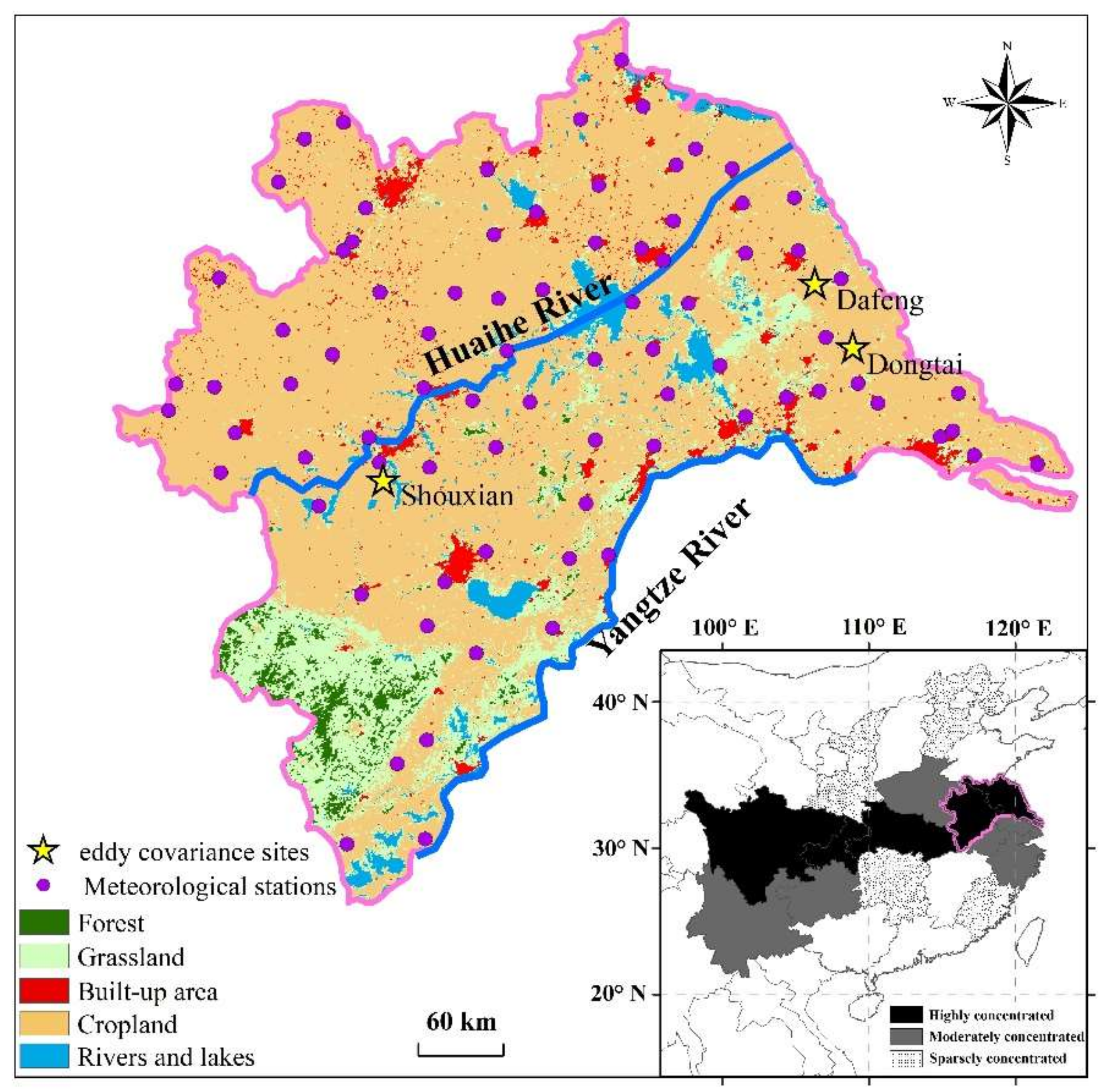
2.1. Study Area

The NYRD is composed of the northern Anhui and Jiangsu provinces and Shanghai, ranging between 114° and 122°E and 29° and 36°N (Figure 1). The NYRD covers an area of 176,960 km2, consisting of 73% cropland, 16% grassland, 5% built-up land, 4% water bodies, and 2% forest (Figure 1). Three EC flux sites were representative of typical rice–wheat-rotation cropland landscapes found in this cropland (Figure 1, inset map) [24,25]. The soil pH value (H2O), soil organic carbon and soil total nitrogen in topsoil (0–0.3 cm) for our study area mainly ranged between 5.5 and 7.2, 1.2, 2, 0.1 and 0.15%, respectively, according to the results of Wei et al. [28]. Here, the winter wheat grows from November to late May. At the beginning of June, the rice paddies are flooded, plowed and harrowed to incorporate the wheat straw residue from the last wheat growing season [29]. Then, one-month-old rice seedlings are transplanted to the leveled field in mid-June and harvested in early November (Figure 2a), which can be indicated by the seasonal dynamics of the 8-day leaf area index (LAI) averaged from 23 weather stations and 3 EC stations during the period of 2014–2018 (Figure 2b). The rice/wheat canopy height can reach about 1–1.2 m at the peak LAI growing seasons. The local climate is sub-tropical monsoon-type, with a mean annual (2014–2018, calculated from the 23 surface meteorological stations in Figure 1) air temperature of 16 °C and rainfall of 1100 mm.

2.2. Data

2.2.1. Eddy Covariance Flux Data

Flux data from three rice–wheat-rotation cropland EC stations within the study area—the Shouxian site in Anhui and the Dongtai and Dafeng sites in Jiangsu—were selected for model training and prediction (Figure 1). At the Shouxian site, the EC sensors were mounted 2.5 m above the ground and consisted of a three-dimensional sonic anemometer (CSAT3, Campbell Scientific Inc., Logan, UT, USA) along with a CO2/H2O open-path infrared gas analyzer (EC 150, Campbell Scientific Inc., Logan, UT, USA). At the Dongtai and Dafeng sites, virtual temperature and wind velocity components were monitored using a three-dimensional sonic anemometer (CSAT3, Campbell Scientific, Inc., Logan, UT, USA). To measure H2O and CO2 density, a fast response open path gas analyzer (LI-7500, LI-COR, Inc., Lincoln, NE, USA) was used. The installation height of the sensors for the Dongtai site was 10 m, whereas for the Dafeng site it was 6.3 m above the ground. As mentioned in the previous studies ([26,27,29]), the three EC sites are relatively flat, with more than 90% of the flux primarily contributed by the cropland. EddyPro 5.2.1 (LI-COR, Inc., Lincoln, NE, USA, 2015) software was applied to calculate hourly CO2 fluxes and to correct for CO2 canopy storage to obtain NEE values. Data pre-processing in the EddyPro software mainly included averaging and statistical tests [30], time lag compensation, double coordinate rotation, spectral correction [31], and Webb–Pearman–Leuning density correction [32]. The poor-quality fluxes (Eddypro quality check flag value = 2) were further discarded. The REddyProc R package (https://www.bgc-jena.mpg.de/bgi/index.php/Services/REddyProcWebRPackage, accessed on 10 July 2021) inputted pre-processed half-hourly EC data and supported further processing [33]. Firstly, a quality-check and filtering were performed based on the relationship between observed flux and friction velocity to discard biased data [34]. Then, the flux data were gap-filled using the marginal distribution sampling approach [35]. NEE was separated into GPP and ecosystem respiration based on the nighttime partitioning algorithms [35]. The gap-filled hourly GPP data were summed to compute cumulative GPP for daily, 8 day, seasonal and annual time resolution for further analysis [36]. Data from these three sites were processed using the same methods. Details of the agricultural practices and processing methods at these three sites can be obtained from the references in Table 1 [26,27,29].

2.2.2. Meteorological Data

Hourly air temperature and relative humidity (RH) at 23 automatic stations were obtained from the China Meteorological Administration for the period of 2014–2018. The hourly vapor pressure deficit (VPD) was estimated with relative humidity and air temperature data following the World Meteorological Organization Commission for Instruments and Methods of Observation Guide conversion equation [37]. The hourly surface downward solar radiation (DSR) ERA5 reanalysis data were provided by the European Center for Medium-Range Weather Forecasts at a 0.25° spatial resolution.

2.2.3. MODIS Data

Land cover maps were available in a 500 m spatial resolution of the MODIS MCD12Q1 product for the year 2016 (Figure 1, ref. [38]). The 16-day Normalized Difference Vegetation Index (NDVI) data during the period of 2014–2018 were obtained from the MODIS MOD13Q1 product with a 250 m resolution [39]. The 8-day fraction of photosynthetically active radiation (FPAR) and LAI data were derived from the 500 m spatial resolution of MODIS MOD15A2H [40]. The MODIS GPP product MOD17A2H (version 6) had a 8-day temporal resolution and 500 m spatial resolution [41]. All of these datasets were downloaded from https://ladsweb.modaps.eosdis.nasa.gov/search/, accessed on 10 July 2021. These MODIS products were quality-controlled to exclude anomalous pixel interference.

2.3. Methods

RF is a fast and flexible machine learning algorithm, which is often used for analyzing the classification and regression tasks [42]. This model can successfully process highly dimensional and multicollinear data, being insensitive to overfitting [43]. The RF model provides a feature-selection tool to identify the importance of the predictor. Feature importance is defined as the contribution of each variable to the model, with important variables showing a greater impact on the model evaluation results [44]. In this section, a GPP prediction model based on RF framework was proposed. The flowchart of estimating and upscaling GPP and calibrating the MOD17A2H GPP product with the RF model is shown in Figure 3, including four steps as follows:
(1)
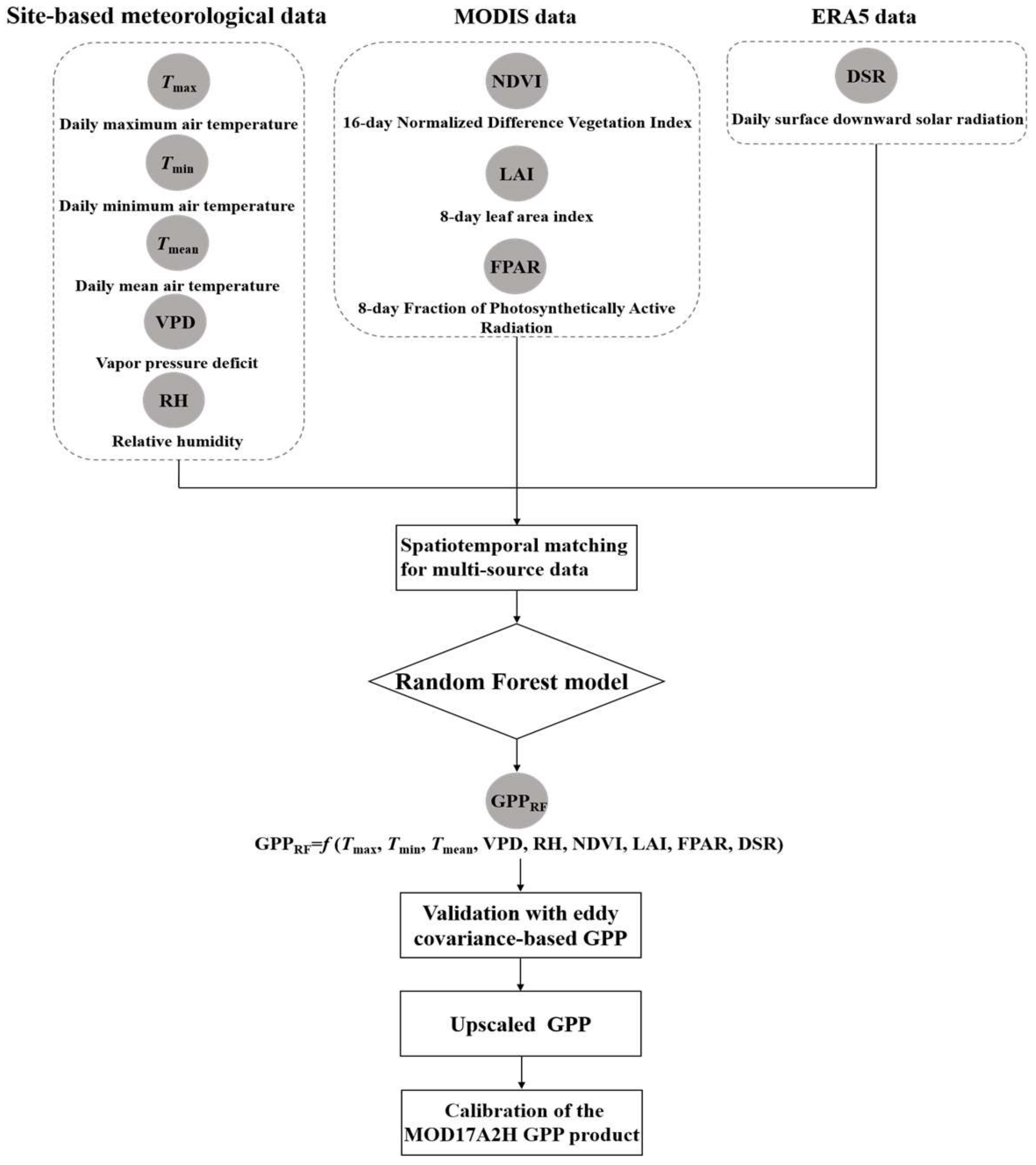
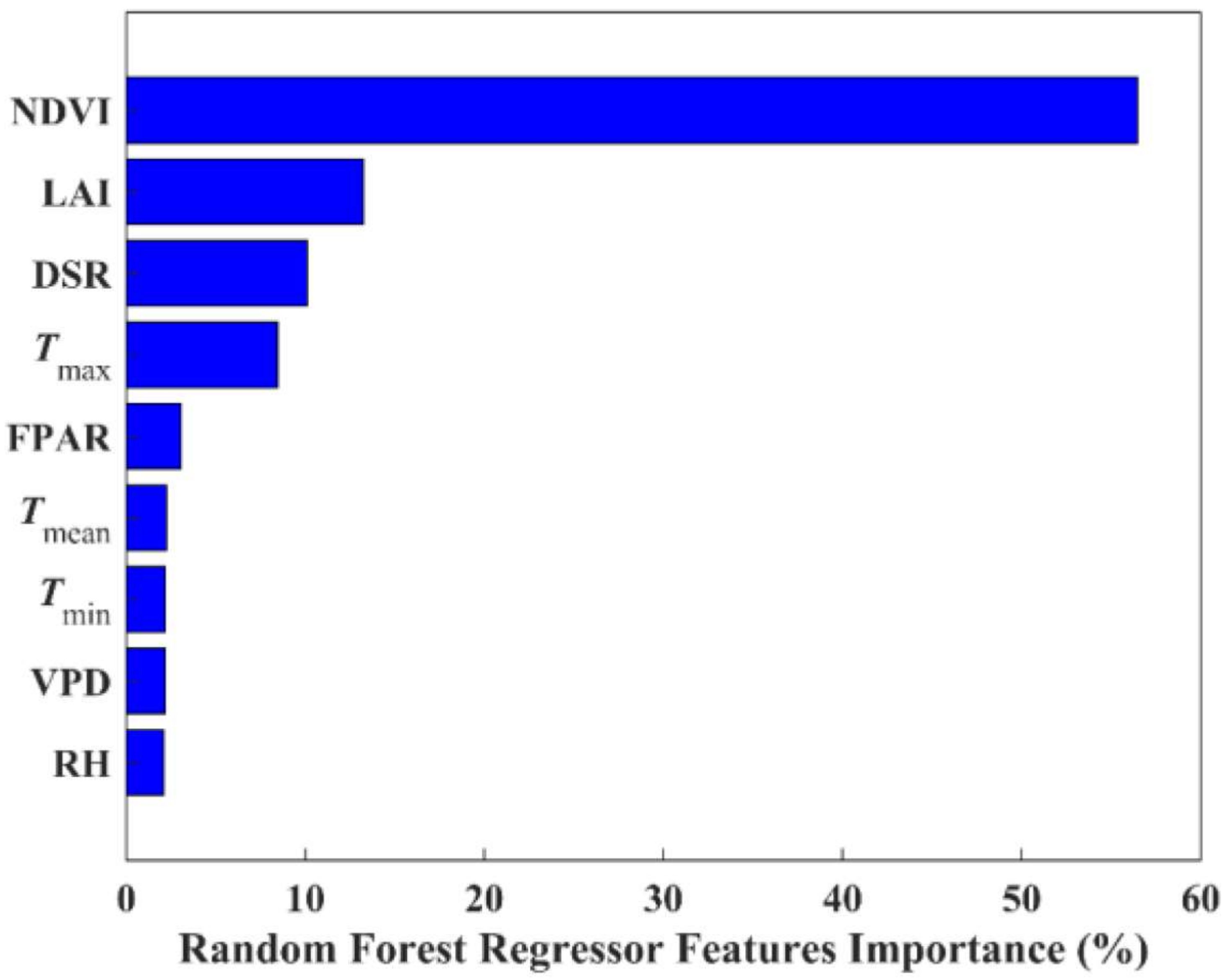
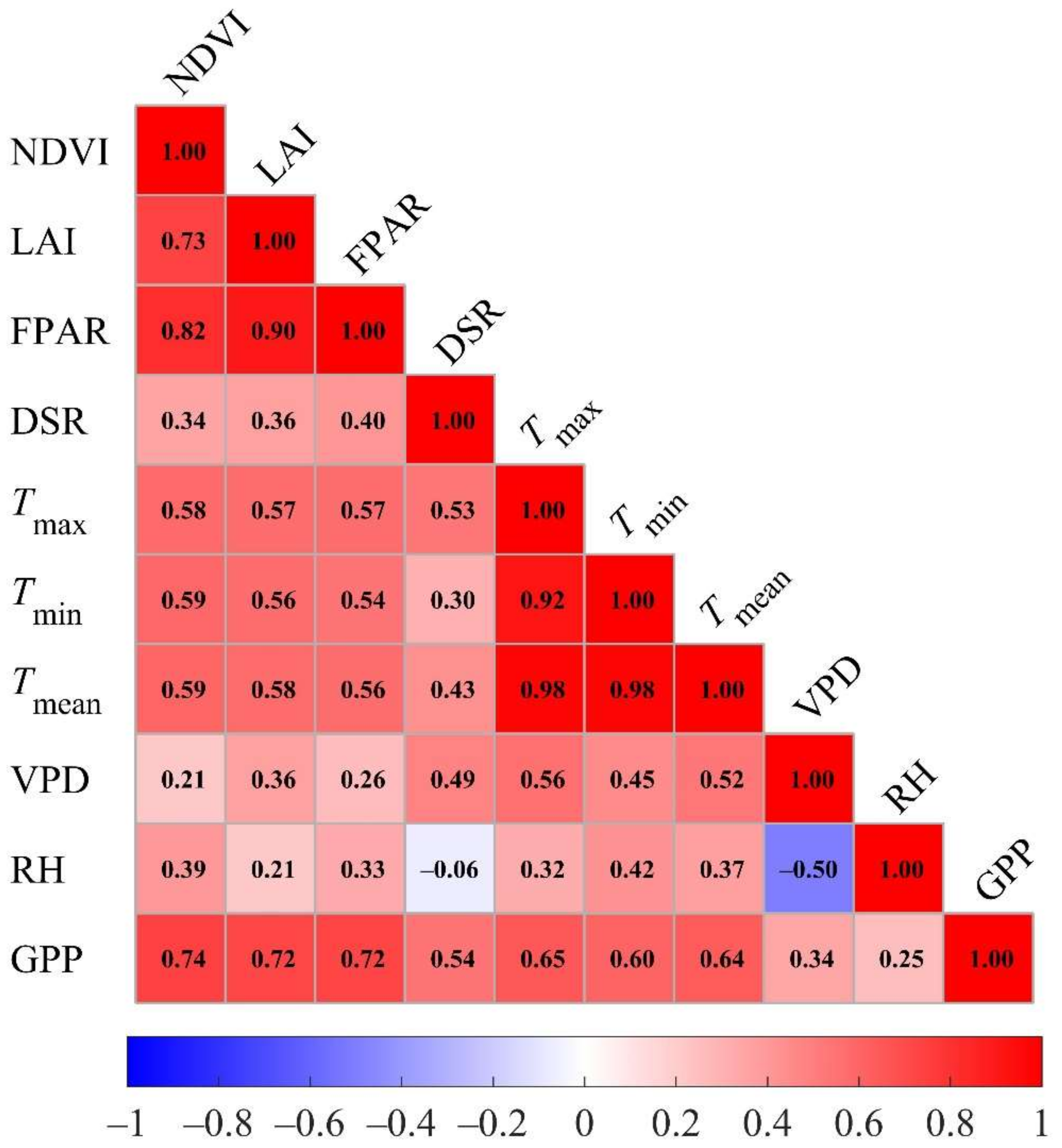
Variable selection and data matching. Crop photosynthesis is a complicated process affected by shortwave radiation, air temperature, vapor pressure deficit, soil edaphoclimatic conditions and fertilization at the canopy scale, etc. Meanwhile, at the ecosystem level, GPP is closely related to light, water and canopy phenology [23,45]. Based on the previous literature as well as our current available data, nine input explanatory variables, NDVI, LAI, FPAR, DSR, daily maximum air temperature (Tmax), daily minimum air temperature (Tmin), daily mean air temperature (Tmean), VPD, and RH, were chosen for predicting the GPP dynamics in the NYRD region. As RF model training requires a large number of samples, MODIS data were linearly interpolated from 8-day/16-day to daily values to match the input parameters, following a previous study by Reitz et al. [19].
(2)
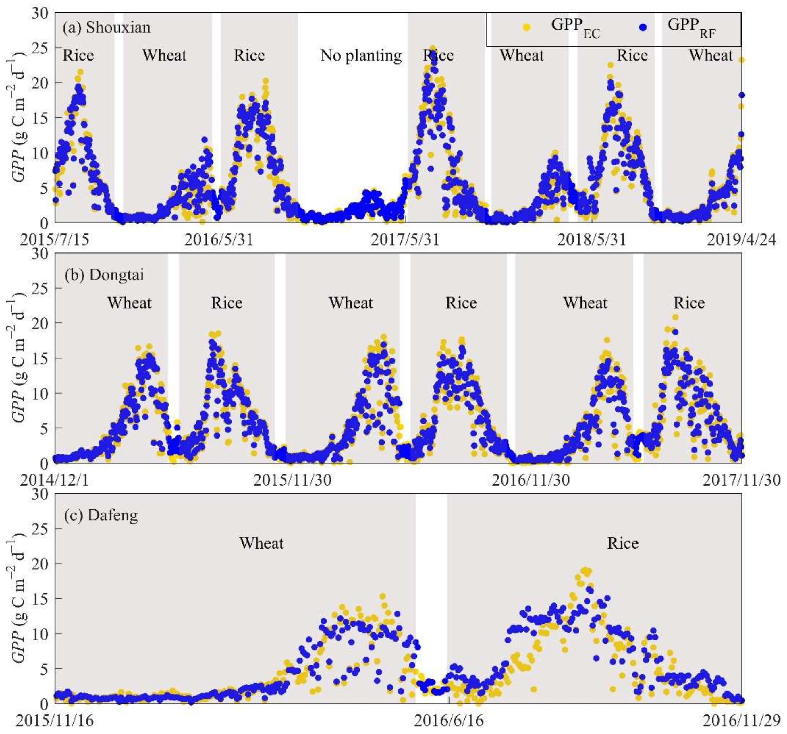
RF model construction, training and testing. In this paper, 90% (the rest 10%) of the EC data at Shouxian and Dongtai during the entire observation period were employed to train (validate) the RF model, and 100% of the EC data at Dafeng were applied to validate the model. The Shouxian and the Dafeng sites were independent of each other with a negligible autocorrelation between them, as these sites are about 300–400 km far away from each other (Figure 1). Here, a 10-fold cross-validation (CV) algorithm was applied to weaken the overfitting [20]. In 10-fold CV experiments, all the training data at the Shouxian and Dongtai sites during the entire observation period were randomly partitioned into ten equal-sized subsamples. Of the ten subsamples, nine subsamples were used as the training data and the remaining one was the testing data. This CV process was repeated ten times, with all ten subsamples used exactly once as the testing data. The ten results from the folds were averaged to produce a single estimation. To select the best model, we adjusted the four hyperparameters of the RF model based on Bayesian optimization [46,47]: the number of trees to grow (n_estimators), the minimum sample number placed in a node prior to the node being split (msplit), maximum number of features considers to split a node (Mfeatures), and the maximum number of levels in each decision tree (Mdepth). Three statistical metrics—the index of agreement (IA) [48], the coefficient of determination (R2), and the root mean square error (RMSE)—were used to examine the simulated performance of the 10-fold CV results. The range of IA is 0–1, and a better correspondence between the observed and modeled results often occurs when it approaches 1 [49]. Therefore, n_estimators = 219, msplit = 2, Mfeatures = 9, and Mdepth = 32 were set for the final RF model.
(3)
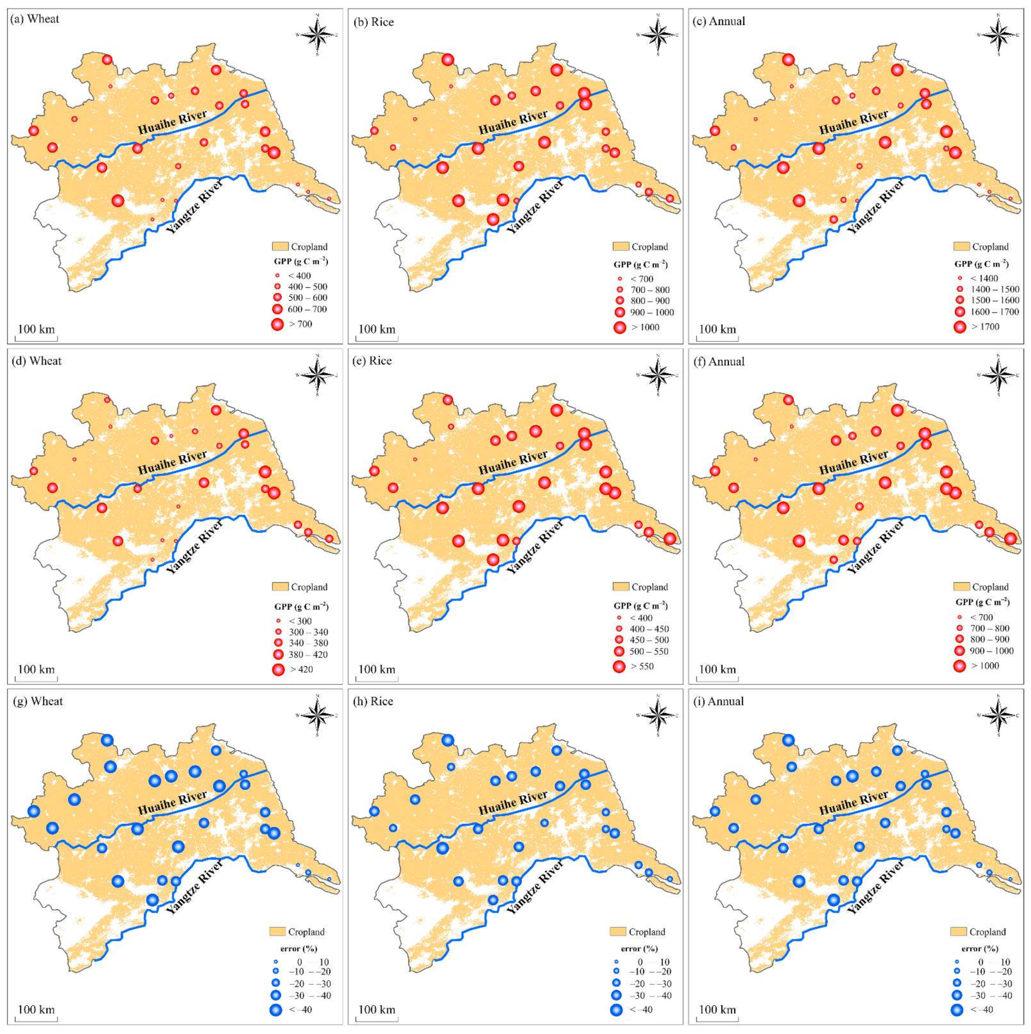
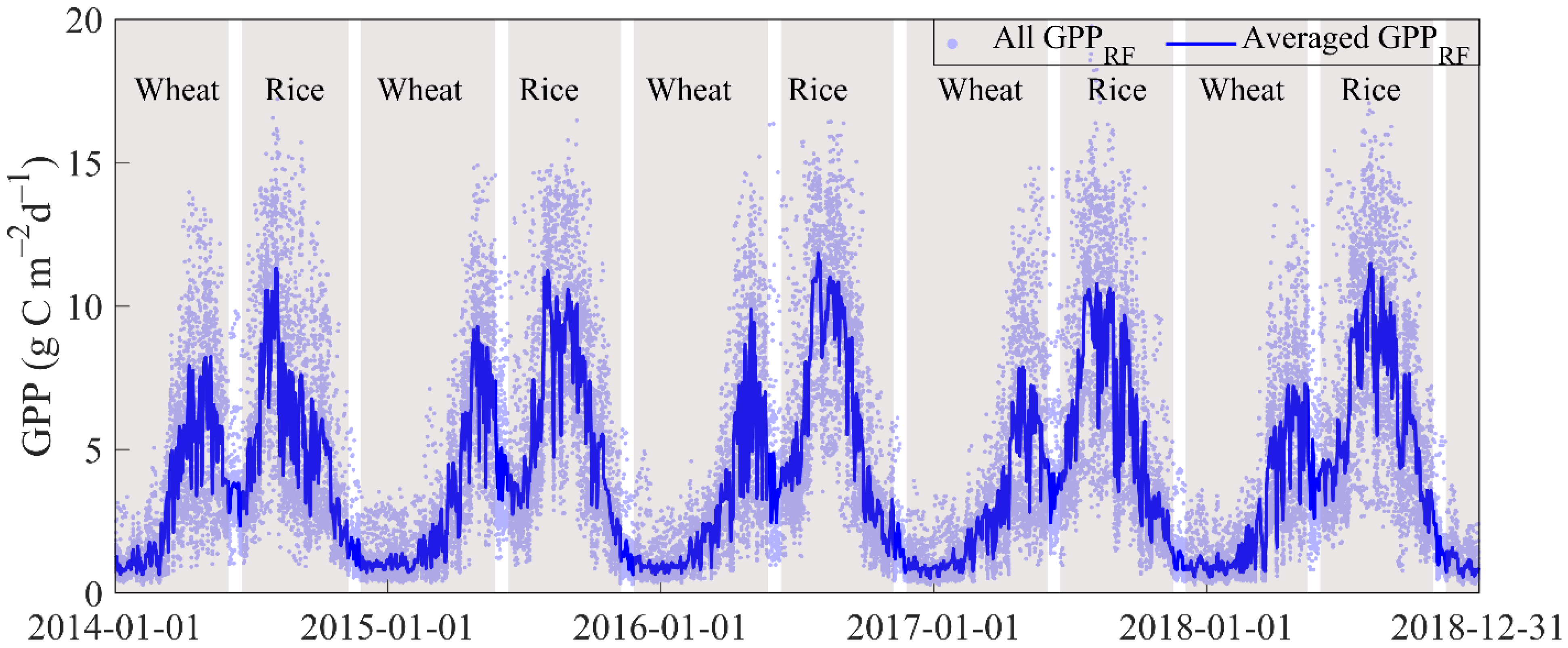
GPP upscaling. The general relationships between GPPRF and explanatory data were first trained at site level, and then applied regionally by using regional surface meteorological stations of explanatory variables as follows: GPPRF VS f (Tmax, Tmin, Tmean, VPD, RH, NDVI, LAI, FPAR, DSR).
(4)
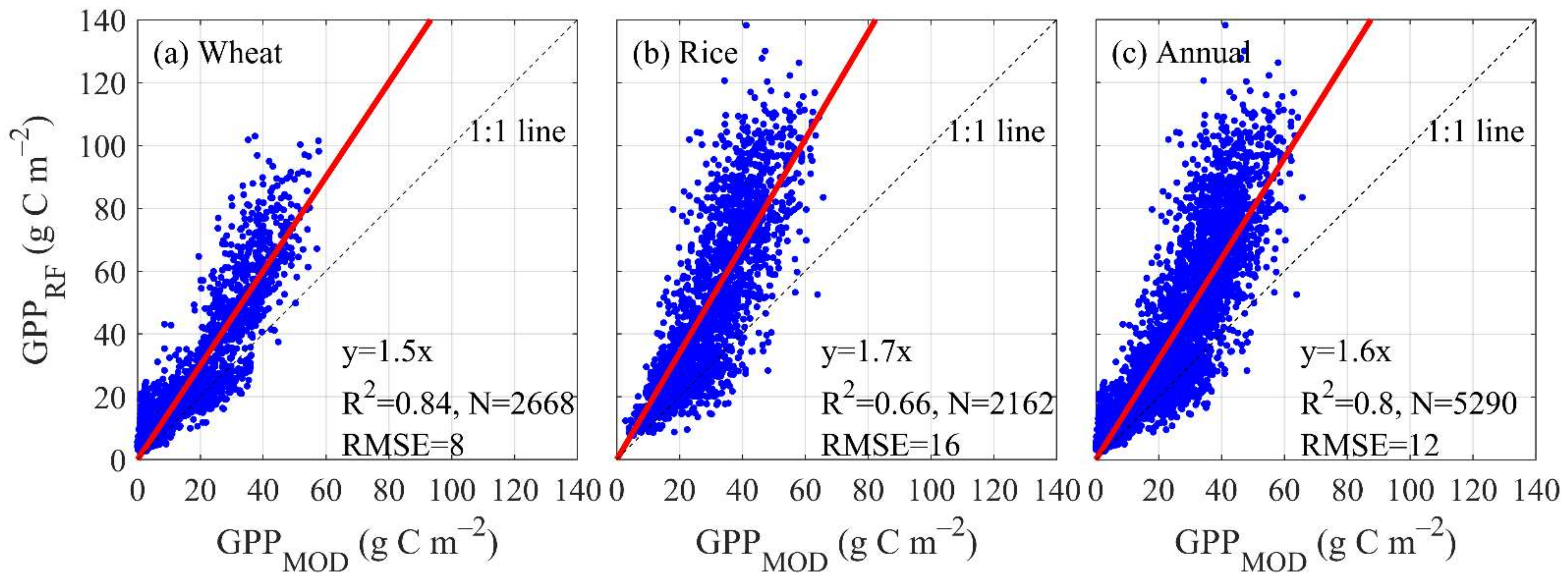
MOD17A2H GPP product calibration. Based on the upscaled results of GPPRF and GPPMOD at the station scale, a relationship between GPPRF and GPPMOD was built. The calibration function was then applied from the site scale to the regional scale.

3. Results

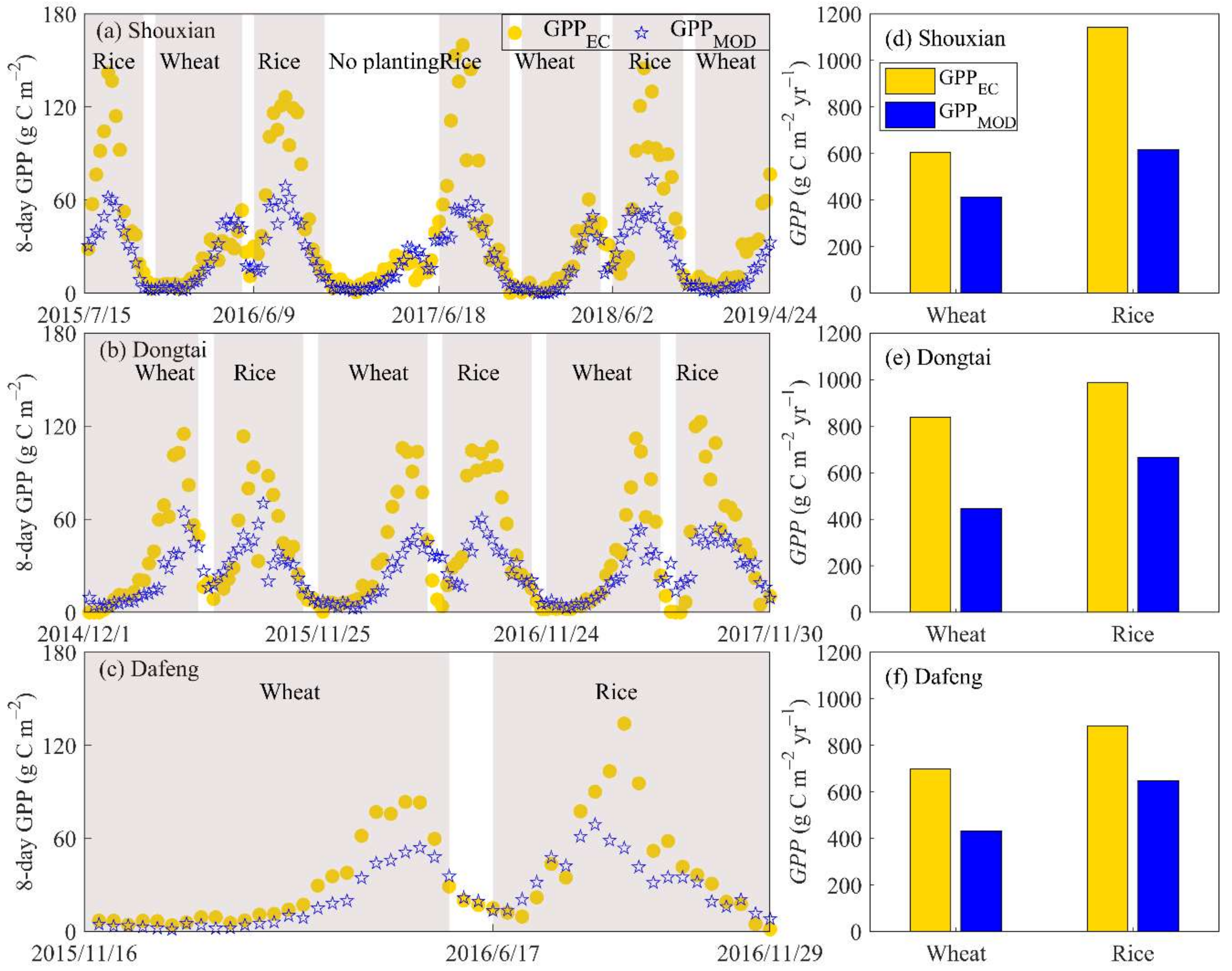
3.1. Intraseasonal Variations of GPP

MOD17A2H GPP has been extensively employed to evaluate the terrestrial carbon balance [1]. However, to have confidence in GPPMOD, it is critical to validate it against in situ measurements [49]. As shown in Figure 4a–c, the 8-day GPPMOD and GPPEC exhibit close agreement in their seasonal patterns, with peaks in July (May) for the rice (wheat) growing seasons across the three rice–wheat-rotation cropland sites. The GPP increases during the no-planting period in 2017 (Figure 4a), mainly due to weed photosynthesis. GPPMOD underestimated GPPEC during the rice (wheat) active growing periods from July to September (from March to May), with IA = 0.56 and RMSE = 47 g C m−2 (IA = 0.61 and RMSE = 29 g C m−2) across the three sites. However, GPPMOD performed well during the intercropping periods from late May to early June (or late November), with IA = 0.77 and RMSE = 8 g C m−2 across the three sites.
The seasonal cumulative GPPEC at the three cropland sites was larger for the summer rice growing seasons (1170, 1066, and 889 g C m−2 for Shouxian, Dongtai and Dafeng, respectively) than for wheat (609, 848 and 701 g C m−2, respectively) (Figure 4d–f). The seasonal cumulative GPPMOD was significantly lower than GPPEC during the wheat growth seasons, with a 32–47% underestimation of the seasonal cumulative GPPEC at the three sites; the seasonal average GPPMOD was 27–47% lower than the seasonal cumulative GPP during the summer rice growth seasons (Figure 4d–f).

3.2. Driving Factors of GPP on a Seasonal Scale

The possible drivers related to the GPP variations in the NYRD are investigated by the RF model in Figure 5 to assess their relative contributions. NDVI was the most important factor in modulating GPP, accounting for 56% of the overall variable importance. As illustrated in Figure 6, GPP showed the strongest positive correlation with NDVI, with the highest Pearson correlation coefficient (r) of 0.74, which was consistent with the variable importance value in Figure 5. In addition to NDVI, there were another three dominant variables—namely, LAI, DSR, Tmax and FPAR, with importance values of 13%, 10%, 8% and 3%, respectively. NDVI and LAI were important indicators of the phase of terrestrial photosynthesis, which tracked well the crop phenological dynamics over time [22,48,50]. DSR and FPAR covaried with light to a large degree—the source of energy for photosynthesis in vegetation [51]. Tmax played a critical role in the chemical reactions of biological processes [17]. In contrast, the impact of Tmean, Tmin, VPD and RH on GPP was not obvious, exhibiting the lowest relative importance, with values of 2, 2, 2 and 2%, respectively. Although FPAR was highly correlated with NDVI (Figure 6), the importance of FPAR was very low in the RF model. This was because NDVI was directly derived from the satellite spectrum, while FPAR was indirectly calculated based on LAI and the physical models. The uncertainties in the MODIS LAI product can be attributed to the input data (surface reflectance or radiation data), model imperfections, and the inversion process [52]. The Pearson correlation coefficient for Tmean (r = 0.64) lay in the range of those for Tmax (r = 0.65) and Tmin (r = 0.60), as Tmean incorporated both day- and nighttime conditions (Figure 6). Generally, all these predictors were involved to different degrees in CO2 exchange processes. Vegetation indices (i.e., NDVI and LAI), related to the phenological properties of the plants, had the greatest influence on GPP variations. In terms of meteorological factors, DSR, Tmax and FPAR carried the information of the light-dependent reactions of photosynthesis, which had a moderate effect on the GPP changes. In particular, Tmean, Tmin, VPD and RH showed weak influences on the GPP cycles.

3.3. Random Forest Model Evaluation
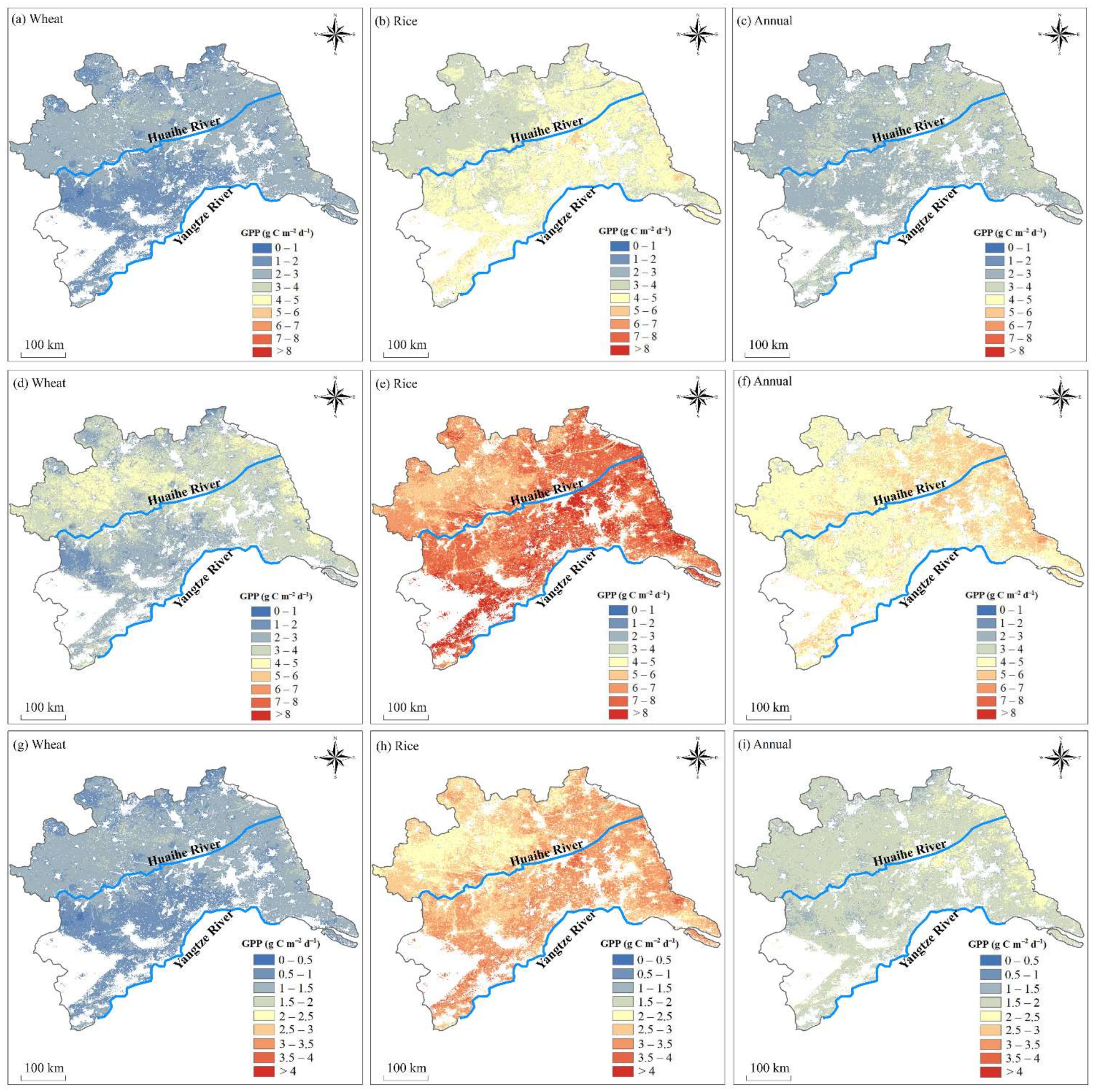
The RF model performed well for both the training (R2 = 0.99, RMSE = 0.42 g C m−2 d−1) and testing (R2 = 0.89, RMSE = 2.8 g C m−2 d−1) datasets (Figure 7a,b). This indicated that the input variables in the RF model were representative and can accurately capture the temporal characteristics of GPP. RF model also proved to be good at the validation site (i.e., Dafeng site), in which the seasonal distributions of GPPRF showed high correlation and coherence with GPPEC (IA = 0.94, Figure 8c). All sites exhibited double peaks, with the peaks during the rice growth season being higher than those during the wheat growth season (Figure 8), which is a common pattern in this double-cropping field. The R2 and RMSE at the validation site (i.e., Dafeng site) were 0.80 and 4.39 g C m−2 d−1 (Figure 7d)—a result that was similar to that across global FLUXNET sites conducted by Tramontana et al. [53], in which the R2 ranged from 0.61 to 0.81. Hence, the RF model was deemed suitable for GPP prediction at unknown stations as well as regional GPP upscaling.

3.4. Upscaled GPP

Figure 9a–c show that the regional RF-modeled cumulative seasonal GPP (GPPRF) averaged from 23 weather stations and 3 EC stations during the period of 2014–2018 was much higher for the rice growth seasons (924 g C m−2) than that for the wheat growth seasons (532 g C m−2). This relationship (cumulative seasonal GPP in the rice growth season > cumulative seasonal GPP in the wheat growth season) was also be confirmed by the GPPMOD in Figure 9d–f. For our study sites, the annual mean for GPPMOD and GPPRF averaged from 23 weather stations and 3 EC stations were 966 g C m−2 and 1548 g C m−2, respectively. Figure 9g–i show the difference between the two GPP products across all sites (relative error at each site as computed by (GPPMOD–GPPRF) × 100/GPPRF) during the period of 2014–2018. Relative errors exhibited negative values across all sites, with −18–−46% for rice growing seasons, −1–−50% for wheat growing seasons and −5–−47% for the whole year, respectively. In general, relative errors during the wheat growing seasons were relatively larger than those during the rice growing seasons/the whole year at most sites (Figure 9g–i).
To examine the spatial consistency of the GPPRF dynamics among the upscaled sites, Figure 10 shows the seasonal variations in GPPRF among 23 weather stations and 3 EC stations during the period of 2014–2018 over the rice–wheat-rotation cropland in the North Yangtze River Delta region. The daily mean GPPRF averaged from 23 weather stations and 3 EC stations during the period of 2014–2018 for wheat was lower than 2 g C m−2 d−1 during the winter extensive bare soil period (December–February). It started to increase in the active tillering stage (March) and reached a maximum of about 8–10 g C m−2 d−1 during the heading stage (late April), and next decreased to around 4 g C m−2 d−1 at harvest. The largest daily GPPRF for rice paddies occurred in late July, with a peak value of about 11 g C m−2 d−1, suggesting that the rice biological activities (e.g., photosynthetic rates) were quite strong at this stage. After that, daily GPPRF decreased to approximately 1 g C m−2 d−1 at rice harvest (Figure 10). Generally, good consistency was found in the seasonal variation among all upscaled sites, exhibiting similarly temporal characteristics of the real GPP over the rice–wheat-rotation system (Figure 4).

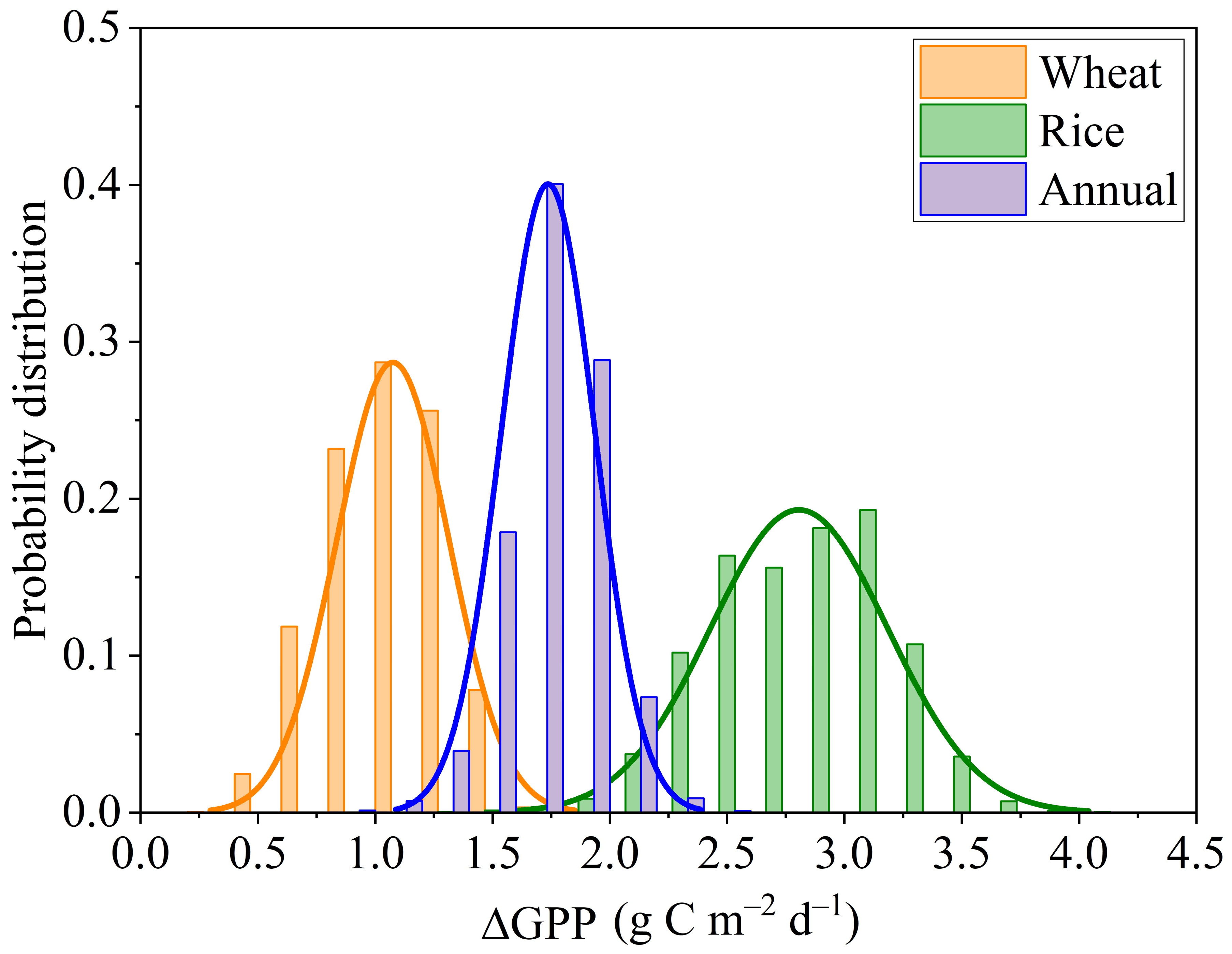
3.5. Calibration of the MOD17A2H GPP Product

Based on the upscaled results of GPPRF and GPPMOD at the station scale in the previous section, the relationship between GPPRF and GPPMOD is shown in Figure 11. Here, the daily GPPRF was aggregated to 8-day sums to match the 8-day GPPMOD product.
Then, the linear relationship between GPPMOD (Figure 12a–c) and the calibrated GPP MOD (GPPCMOD) (Figure 12d–f) at the grid scale was established as follows:
G P P C M O D = 1.5 × G P P M O D , f o r   w h e a t 1.7 × G P P M O D , f o r   r i c e 1.6 × G P P M O D , f o r   a n n u a l
Both GPPMOD and GPPCMOD exhibited a higher value during the rice growth seasons than that during the wheat growth seasons. The annual mean GPP in most parts of the NYRD varied from 2 to 4 g C m−2 d−1 for GPPMOD and 4 to 6 g C m−2 d−1 for GPPCMOD, with the higher values in the eastern coastal areas of the NYRD (Figure 12c,f). Here, sea–land breezes prevail, carrying rainfall and water resources sufficient to favor crop growth. Figure 12g–i show the seasonal mean of the error ranges of daily GPP (∆GPP, as computed by subtracting GPPMOD (Figure 12a–c) from GPPCMOD (Figure 12d–f)) during the period of 2014–2018. ∆GPP in most parts of the NYRD ranged between 2 and 4 g C m−2 d−1 during the rice growing seasons, while they were smaller (i.e., 0–1.5 g C m−2 d−1) for wheat. The probability density function (PDF) of ∆GPP in the NYRD is shown in Figure 13. The PDF of ∆GPP varies seasonally, which play a pivotal role in regulating the carbon dynamics in the NYRD. Rice paddies had a broader distribution in the peak PDF of the mean ∆GPP than that for wheat fields, i.e., between 0.75 and 1.25 g C m−2 d−1 during the wheat growth seasons, between 2.5 and 3.25 g C m−2 d−1 during the rice growth seasons, and around 1.75 g C m−2 d−1 for the annual mean.

4. Discussion

4.1. Complexity of the Drivers of Spatio-Temporal Variation in GPP

In this work, three rice–wheat-rotation cropland EC sites were quantified and used to explore the complexity of the drivers of spatio-temporal variation in GPP. In order to eliminate the errors induced by instrument measurements, Table 2 only summarized GPP values in EC-based literatures. The cumulative GPP for the wheat fields ranged from 609 to 848 g C m−2 in eastern China, which was equivalent to that reported in India (621 g C m−2, ref. [54]) but lower than that reported in Germany (1241 g C m−2, ref. [55]) and northern China (1174 g C m−2, ref. [56]). The total seasonal GPP during the rice growing season in eastern China (889–1170 g C m−2) was higher than that in India (811 g C m−2, ref. [57]) and the Philippines (778 g C m−2, ref. [51]). The discrepancy in the cumulative seasonal GPP among the previous studies is probably because of the difference in local meteorological conditions (e.g., precipitation, air temperature, and photosynthetically active radiation) and phenology (e.g., growth duration, NDVI and LAI) [55,56,57]. For example, the summer rice growing season was warmer (23–24 °C in eastern China) and received more precipitation (735–1028 mm in eastern China, Table 2) as compared with the winter wheat growing season. The mean seasonal GPP for rice paddies (889–1170 g C m−2) was obviously higher than those for wheat fields (609–848 g C m−2) in eastern China, mostly because of the different crop growth conditions. Furthermore, values of 609–848 g C m−2 for winter wheat fields in eastern China were lower than the value of 1174 g C m−2 in northern China, mainly because the growth duration of winter wheat in northern China is generally longer [56].
In addition to the meteorological factors and phenology, crop management (e.g., fertilizer) and edaphoclimatic conditions (e.g., soil temperature, soil water content and microbial populations) also have influences on the GPP dynamics. The fertilization time for wheat and rice is basically fixed (Figure 2) during the sowing period (early June for rice and middle November for wheat) and the tillering period (early July for rice and late February for wheat). Chen et al. [15] reported that the basic fertilizer applied during the rice/wheat sowing period had the most remarkable effect, with an increase in GPP reaching 2–3 g C m–2d–1 over 8 days. Spraying leaf fertilization during the crop tillering stages had a minor effect on GPP, with an increase in GPP up to 1–2 g C m–2d–1 over 8 days. Edaphoclimatic conditions (such as soil temperature and soil moisture) varied seasonally, modulating the GPP dynamics [18]. However, detailed information about the in situ fertilization and the edaphoclimatic conditions was not available for us to input into our RF models. Considering the importance of these factors, nevertheless, we cannot ignore the potential influence of the crop management or edaphoclimatic conditions.

4.2. Potential Discrepancy between GPPEC and GPPMOD

Figure 4 shows the inconsistency between GPPMOD and GPPEC at the three sites, which can be attributed to three aspects: (a) input parameters such as FPAR data and meteorological conditions [49]; (b) the uncertainties in the MOD17A2H GPP algorithm [2]; and (c) the spatial mismatch between remotely sensed pixels and EC footprints [58,59]. In the past few decades, a wide network of sites have been established across various ecosystems and climate regions; for example, AmeriFlux, Integrated Carbon Observation System, National Ecological Observatory Network, and FluxNet [60,61]. These EC sites provide potential opportunities to annually update the cropland sites in the land cover maps, redefine the MOD17 cropland parameters and greatly improve GPPMOD at regional or even global scales. To the best of our knowledge, China has the largest area of the rice–wheat-rotation croplands in the world. In China, these croplands are distributed widely along the Yangtze River Basin (Figure 1, inset map), covering around 13 Mha in total [24]. This rotation cropland system is a non-negligible part of the agroecosystem. While the MOD17 algorithm defines only 11 land cover classes, i.e., one type of cropland, one type of woodland, two types of grasslands, two types of shrubland and five types of forests [49]. Therefore, the large discrepancy between GPPMOD and GPPEC over the rice–wheat-rotation cropland indicates that the parameters in the MOD17 product should be modified and more types of cropland (e.g., double-cropping or mixed-cropping systems) should be defined.
Meanwhile, the MOD17 GPP product has a fine resolution with 500 m, and so the high-quality MOD17 GPP product can be employed to accurately assess the ecosystem’s carbon cycle and agricultural productions. In particular, out-of-academy precision agriculture or commercialized precision agriculture put forward higher requirements for the accuracy evaluation of GPP products. Nowadays, EC-based calibration of MODIS products is a common method. In the present work, due to the study being limited to three EC sites over rotation cropland areas in eastern China, the observations cannot be used to stand for the whole area. Therefore, we proposed the machine learning-based GPP prediction model for 23 meteorological sites by using multi-source data to derive more virtual EC sites (23 sites) over the whole area, which can offer more ground-based GPP samples for calibrating MOD17 GPP. Generally, the simulations of the RF-based GPP models show a better performance with respect to other machine learning methods (e.g., Decision Tree Regression, support vector machine, artificial neural network, and deep belief network, referring to Figures S1–S4 in the Supplementary Materials), which is consistent with the results in Yu et al. [23]. In our present work, thus, RF-based upscaling and calibrating methods are more suitable over large-scale agroecosystem areas if EC measurements, meteorological observations and MODIS data are available.

5. Conclusions

In this study, the GPP estimated from EC flux measurements over rice–wheat-rotation cropland can represent the amount of carbon uptake by the main land cover type in the NYRD area. To obtain multiple samples for calibration of the MOD17A2H GPP product, a RF model for estimating GPP was designed by integrating multi-source satellite retrievals and in situ ground observations during the period of 2014–2018 over the rice–wheat double-cropping fields of eastern China. The RF model showed that multiple co-acting factors (NDVI, LAI, DSR, Tmax, and FPAR) modulate GPP dynamics. GPPRF performed well when compared with GPPEC, with a R2 of 0.99 and RMSE of 0.42 g C m−2 d−1, indicating these explanatory variables are reasonably representative and reliable for regional GPP upscaling. The regional upscaled cumulative seasonal GPPRF in rice paddies (924 g C m−2) was roughly two times higher than that in a wheat field (532 g C m−2) at the station scale, probably because of the much longer growing season and lower LAI of wheat. Compared with GPPEC, this indicates that GPPMOD underestimates GPP during the active crop growth stages but performs well during the crop rotation periods. Based on the upscaled results of GPPRF at the station scale, the functional relationship between GPPMOD and GPPRF at the grid scale was established to calibrate the GPPMOD. The error range of ∆GPP (GPPRF minus GPPMOD) was higher for rice paddies than for wheat fields, i.e., between 0.75 and 1.25 g C m−2 d−1 during the wheat growth seasons, between 2.5 and 3.25 g C m−2 d−1 during the rice growth seasons, along with an annual mean of 1.75–2 g C m−2 d−1.
To sum up, the GPP in rice–wheat-rotation agroecosystems is considerably diverse and varies with the seasons. Our findings are potentially applicable in terms of the climate response of greenhouse gases over wide-scale cropland areas. Our research demonstrates that RF machine learning is a powerful and expedient modeling tool for estimating and even calibrating the MODIS GPP product. In future, it would be worthwhile using global FLUXNET data, multi-source satellite observations and machine learning methods to simulate the GPP in more ecosystem types (e.g., grassland and forests) and climate zones at large scales to fully understand the nature of global carbon dynamics.

Supplementary Materials

The following are available online at https://0-www-mdpi-com.brum.beds.ac.uk/article/10.3390/rs13214229/s1, Figure S1: Scatter density plots results for the support vector machine model in predicting gross primary productivity in the (a) 10-fold cross-validation training set, (b) 10-fold cross-validation testing set, (c) validation by the rest samples at Shouxian and Dongtai sites, and (d) validation by all samples at Dafeng site, Figure S2: Scatter density plots results for the Decision Tree Regression model in predicting gross primary productivity in the (a) 10-fold cross-validation training set, (b) 10-fold cross-validation testing set, (c) validation by the rest samples at Shouxian and Dongtai sites, and (d) validation by all samples at Dafeng site, Figure S3: Scatter density plots results for the deep belief network model in predicting gross primary productivity in the (a) 10-fold cross-validation training set, (b) 10-fold cross-validation testing set, (c) validation by the rest samples at Shouxian and Dongtai sites, and (d) validation by all samples at Dafeng site, Figure S4: Scatter density plots results for the artificial neural network model in predicting gross primary productivity in the (a) 10-fold cross-validation training set, (b) 10-fold cross-validation testing set, (c) validation by the rest samples at Shouxian and Dongtai sites, and (d) validation by all samples at Dafeng site.

Author Contributions

Conceptualization, Z.D. and Y.Y.; methodology, Z.D., Y.Y. and S.Z.; software, Z.D., S.Z. and L.Z.; validation, Z.D., Y.Y. and Z.G.; formal analysis, Z.D., Y.Y., S.Z., Z.G., L.Z., S.F. and J.Y.; data curation, Y.Y. and Z.G.; writing—original draft preparation, Z.D. and Y.Y.; writing—review and editing, Z.D., Y.Y. and Z.G. All authors have read and agreed to the published version of the manuscript.

Funding

This work was funded by the National Natural Science Foundation of China (Grant: 41875013).

Institutional Review Board Statement

Not applicable.

Informed Consent Statement

Not applicable.

Data Availability Statement

MODIS products used in this paper can be downloaded from https://ladsweb.modaps.eosdis.nasa.gov/search/, accessed on 10 July 2021. ERA5 reanalysis data is from the Copernicus Climate Change Service at https://cds.climate.copernicus.eu/cdsapp#!/dataset/reanalysis-era5-single-levels?tab=form, accessed on 10 July 2021. The data of automatic stations and eddy covariance flux data are not available to the public. Please direct any inquiries regarding the data to the first author ([email protected]).

Acknowledgments

We acknowledge Hongsheng Zhang at Peking University for providing the eddy covariance data at the Dafeng site. We are very grateful to three anonymous reviewers for their careful review and valuable comments, which led to a substantial improvement of the paper.

Conflicts of Interest

The authors declare no conflict of interest.

References

  1. Zhu, X.Y.; Pei, Y.Y.; Zheng, Z.P.; Dong, J.W.; Zhang, Y.; Wang, J.B.; Chen, L.J.; Doughty, R.B.; Zhang, G.L.; Xiao, X.M. Underestimates of Grassland Gross Primary Production in MODIS Standard Products. Remote Sens. 2018, 10, 1771. [Google Scholar] [CrossRef] [Green Version]
  2. Wang, L.; Zhu, H.; Lin, A.; Zou, L.; Qin, W.; Du, Q. Evaluation of the Latest MODIS GPP Products across Multiple Biomes Using Global Eddy Covariance Flux Data. Remote Sens. 2017, 9, 418. [Google Scholar] [CrossRef] [Green Version]
  3. Wood, S.; Sebastian, K.; Scherr, S. Pilot Analysis of Global Ecosystems: Agroecosystems; WRI: Washington, DC, USA, 2000. [Google Scholar]
  4. Malmström, C.M.; Thompson, M.V.; Juday, G.P.; Los, S.O.; Randerson, J.T.; Field, C.B. Interannual variation in global-scale net primary production: Testing model estimates. Glob. Biogeochem. Cycles 1997, 11, 367–392. [Google Scholar] [CrossRef] [Green Version]
  5. Xie, X.Y.; Li, A.N.; Tan, J.B.; Jin, H.A.; Nan, X.; Zhang, Z.J.; Bian, J.H.; Lei, G.B. Assessments of gross primary productivity estimations with satellite data-driven models using eddy covariance observation sites over the northern hemisphere. Agric. For. Meteorol. 2020, 280, 14. [Google Scholar] [CrossRef]
  6. Baldocchi, D.D. Assessing the eddy covariance technique for evaluating carbon dioxide exchange rates of ecosystems: Past, present and future. Glob. Change Biol. 2003, 9, 479–492. [Google Scholar] [CrossRef] [Green Version]
  7. Lasslop, G.; Reichstein, M.; Papale, D.; Richardson, A.D.; Arneth, A.; Barr, A.; Stoy, P.; Wohlfahrt, G. Separation of net ecosystem exchange into assimilation and respiration using a light response curve approach: Critical issues and global evaluation. Glob. Change Biol. 2010, 16, 187–208. [Google Scholar] [CrossRef] [Green Version]
  8. John, R.; Chen, J.; Noormets, A.; Xiao, X.; Xu, J.; Lu, N.; Chen, S. Modelling gross primary production in semi-arid Inner Mongolia using MODIS imagery and eddy covariance data. Int. J. Remote Sens. 2013, 34, 2829–2857. [Google Scholar] [CrossRef]
  9. Lee, B.; Kim, N.; Kim, E.-S.; Jang, K.; Kang, M.; Lim, J.-H.; Cho, J.; Lee, Y. An Artificial Intelligence Approach to Predict Gross Primary Productivity in the Forests of South Korea Using Satellite Remote Sensing Data. Forests 2020, 11, 1000. [Google Scholar] [CrossRef]
  10. Reeves, M.C.; Zhao, M.; Running, S.W. Usefulness and limits of MODIS GPP for estimating wheat yield. Int. J. Remote Sens. 2005, 26, 1403–1421. [Google Scholar] [CrossRef]
  11. Post, H.; Hendricks Franssen, H.J.; Han, X.; Baatz, R.; Montzka, C.; Schmidt, M.; Vereecken, H. Evaluation and uncertainty analysis of regional-scale CLM4.5 net carbon flux estimates. Biogeosciences 2018, 15, 187–208. [Google Scholar] [CrossRef] [Green Version]
  12. Wang, J.W.; Denning, A.S.; Lu, L.X.; Baker, I.T.; Corbin, K.D.; Davis, K.J. Observations and simulations of synoptic, regional, and local variations in atmospheric CO2. J. Geophys. Res.-Atmos. 2007, 112, 7410. [Google Scholar] [CrossRef] [Green Version]
  13. Ueyama, M.; Ichii, K.; Iwata, H.; Euskirchen, E.S.; Zona, D.; Rocha, A.V.; Harazono, Y.; Iwama, C.; Nakai, T.; Oechel, W.C. Upscaling terrestrial carbon dioxide fluxes in Alaska with satellite remote sensing and support vector regression. J. Geophys. Res. Biogeosci. 2013, 118, 1266–1281. [Google Scholar] [CrossRef]
  14. Cutler, D.R.; Edwards, T.C., Jr.; Beard, K.H.; Cutler, A.; Hess, K.T.; Gibson, J.; Lawler, J.J. Random Forests for Classification in Ecology. Ecology 2007, 88, 2783–2792. [Google Scholar] [CrossRef] [PubMed]
  15. Jung, M.; Reichstein, M.; Margolis, H.A.; Cescatti, A.; Richardson, A.D.; Arain, M.A.; Arneth, A.; Bernhofer, C.; Bonal, D.; Chen, J.; et al. Global patterns of land-atmosphere fluxes of carbon dioxide, latent heat, and sensible heat derived from eddy covariance, satellite, and meteorological observations. J. Geophys. Res. Biogeosci. 2011, 116, 1566. [Google Scholar] [CrossRef] [Green Version]
  16. Dou, X.; Yang, Y.; Luo, J. Estimating Forest Carbon Fluxes Using Machine Learning Techniques Based on Eddy Covariance Measurements. Sustainability 2018, 10, 203. [Google Scholar] [CrossRef] [Green Version]
  17. Tramontana, G.; Migliavacca, M.; Jung, M.; Reichstein, M.; Keenan, T.F.; Camps-Valls, G.; Ogee, J.; Verrelst, J.; Papale, D. Partitioning net carbon dioxide fluxes into photosynthesis and respiration using neural networks. Glob. Change Biol. 2020, 26, 5235–5253. [Google Scholar] [CrossRef]
  18. Zeng, J.; Matsunaga, T.; Tan, Z.-H.; Saigusa, N.; Shirai, T.; Tang, Y.; Peng, S.; Fukuda, Y. Global terrestrial carbon fluxes of 1999–2019 estimated by upscaling eddy covariance data with a random forest. Sci. Data 2020, 7, 313. [Google Scholar] [CrossRef]
  19. Reitz, O.; Graf, A.; Schmidt, M.; Ketzler, G.; Leuchner, M. Upscaling Net Ecosystem Exchange Over Heterogeneous Landscapes With Machine Learning. J. Geophys. Res. Biogeosci. 2021, 126, 5814. [Google Scholar] [CrossRef]
  20. Cai, J.C.; Xu, K.; Zhu, Y.H.; Hu, F.; Li, L.H. Prediction and analysis of net ecosystem carbon exchange based on gradient boosting regression and random forest. Appl. Energy 2020, 262, 114566. [Google Scholar] [CrossRef]
  21. Chen, Y.; Shen, W.; Gao, S.; Zhang, K.; Wang, J.; Huang, N. Estimating deciduous broadleaf forest gross primary productivity by remote sensing data using a random forest regression model. J. Appl. Remote Sens. 2019, 13, e038502. [Google Scholar] [CrossRef]
  22. Tramontana, G.; Ichii, K.; Camps-Valls, G.; Tomelleri, E.; Papale, D. Uncertainty analysis of gross primary production upscaling using Random Forests, remote sensing and eddy covariance data. Remote Sens. Environ. 2015, 168, 360–373. [Google Scholar] [CrossRef]
  23. Yu, T.; Zhang, Q.; Sun, R. Comparison of Machine Learning Methods to Up-Scale Gross Primary Production. Remote Sens. 2021, 13, 2448. [Google Scholar] [CrossRef]
  24. Timsina, J.; Connor, D.J. Productivity and management of rice–wheat cropping systems: Issues and challenges. Field Crop. Research. 2001, 69, 93–132. [Google Scholar] [CrossRef]
  25. Chen, C.; Li, D.; Gao, Z.; Tang, J.; Guo, X.; Wang, L.; Wan, B. Seasonal and interannual variations of carbon exchange over a rice-wheat rotation system on the North China Plain. Adv. Atmos. Sci. 2015, 32, 1365–1380. [Google Scholar] [CrossRef]
  26. Duan, Z.; Yang, Y.; Wang, L.; Liu, C.; Fan, S.; Chen, C.; Tong, Y.; Lin, X.; Gao, Z. Temporal characteristics of carbon dioxide and ozone over a rural-cropland area in the Yangtze River Delta of eastern China. Sci. Total Environ. 2021, 757, e143750. [Google Scholar] [CrossRef] [PubMed]
  27. Ge, H.; Zhang, H.; Zhang, H.; Cai, X.; Song, Y.; Kang, L. The characteristics of methane flux from an irrigated rice farm in East China measured using using the eddy covariance method. Agric. For. Meteorol. 2018, 249, 228–238. [Google Scholar] [CrossRef]
  28. Shangguan, W.; Dai, Y.; Liu, B.; Zhu, A.; Duan, Q.; Wu, L.; Ji, D.; Ye, A.; Yuan, H.; Zhang, Q.; et al. A China data set of soil properties for land surface modeling. J. Adv. Model. Earth Syst. 2013, 5, 212–224. [Google Scholar] [CrossRef]
  29. Duan, Z.; Grimmond, C.; Gao, C.Y.; Sun, T.; Liu, C.; Wang, L.; Li, Y.; Gao, Z. Seasonal and interannual variations in the surface energy fluxes of a rice–wheat rotation in Eastern China. J. Appl. Meteorol. Climatol. 2021, 60, 877–891. [Google Scholar] [CrossRef]
  30. Anapalli, S.S.; Fisher, D.K.; Reddy, K.N.; Krutz, J.L.; Pinnamaneni, S.R.; Sui, R. Quantifying water and CO2 fluxes and water use efficiencies across irrigated C3 and C4 crops in a humid climate. Sci. Total Environ. 2019, 663, 338–350. [Google Scholar] [CrossRef]
  31. Moncrieff, J.; Clement, R.; Finnigan, J.; Meyers, T. Averaging, Detrending, and Filtering of Eddy Covariance Time Series. In Handbook of Micrometeorology: A Guide for Surface Flux Measurement and Analysis; Lee, X., Massman, W., Law, B., Eds.; Springer: Dordrecht, The Netherlands, 2005; pp. 7–31. [Google Scholar]
  32. Webb, E.K.; Pearman, G.I.; Leuning, R. Correction of flux measurements for density effects due to heat and water vapour transfer. Q. J. R. Meteorol. Soc. 1980, 106, 85–100. [Google Scholar] [CrossRef]
  33. Wutzler, T.; Lucas-Moffat, A.; Migliavacca, M.; Knauer, J.; Sickel, K.; Sigut, L.; Menzer, O.; Reichstein, M. Basic and extensible post-processing of eddy covariance flux data with REddyProc. Biogeosciences 2018, 15, 5015–5030. [Google Scholar] [CrossRef] [Green Version]
  34. Papale, D.; Reichstein, M.; Aubinet, M.; Canfora, E.; Bernhofer, C.; Kutsch, W.; Longdoz, B.; Rambal, S.; Valentini, R.; Vesala, T.; et al. Towards a standardized processing of Net Ecosystem Exchange measured with eddy covariance technique: Algorithms and uncertainty estimation. Biogeosciences 2006, 3, 571–583. [Google Scholar] [CrossRef] [Green Version]
  35. Reichstein, M.; Falge, E.; Baldocchi, D.; Papale, D.; Aubinet, M.; Berbigier, P.; Bernhofer, C.; Buchmann, N.; Gilmanov, T.; Granier, A.; et al. On the separation of net ecosystem exchange into assimilation and ecosystem respiration: Review and improved algorithm. Glob. Change Biol. 2005, 11, 1424–1439. [Google Scholar] [CrossRef]
  36. Wagle, P.; Gowda, P.H.; Northup, B.K.; Neel, J.P.S.; Starks, P.J.; Turner, K.E.; Moriasi, D.N.; Xiao, X.; Steiner, J.L. Carbon dioxide and water vapor fluxes of multi-purpose winter wheat production systems in the U.S. Southern Great Plains. Agric. For. Meteorol. 2021, 310, 108631. [Google Scholar] [CrossRef]
  37. Yang, D.; Xu, X.; Xiao, F.; Xu, C.; Luo, W.; Tao, L. Improving modeling of ecosystem gross primary productivity through re-optimizing temperature restrictions on photosynthesis. Sci. Total Environ. 2021, 788, 147805. [Google Scholar] [CrossRef]
  38. Friedl, M.; Sulla-Menashe, D. MCD12Q1 MODIS/Terra+Aqua Land Cover Type Yearly L3 Global 500m SIN Grid V006. NASA EOSDIS Land Process. DAAC; 2019. Available online: https://lpdaac.usgs.gov/products/mcd12q1v006/ (accessed on 10 July 2021). [CrossRef]
  39. Didan, K. MOD13Q1 MODIS/Terra Vegetation Indices 16-Day L3 Global 250m SIN Grid V006. NASA EOSDIS Land Process. DAAC; 2015. Available online: https://lpdaac.usgs.gov/products/mod13q1v006 (accessed on 10 July 2021). [CrossRef]
  40. Myneni, R.; Knyazikhin, Y.; Park, T. MOD15A2H MODIS/Terra Leaf Area Index/FPAR 8-Day L4 Global 500m SIN Grid V006. NASA EOSDIS Land Process. DAAC; 2015. Available online: https://lpdaac.usgs.gov/products/mod15a2hv006/ (accessed on 10 July 2021). [CrossRef]
  41. Running, S.; Mu, Q.; Zhao, M. MOD17A2H MODIS/Terra Gross Primary Productivity 8-Day L4 Global 500m SIN Grid V006. NASA EOSDIS Land Process. DAAC; 2015. Available online: https://lpdaac.usgs.gov/products/mod17a2hv006/ (accessed on 10 July 2021). [CrossRef]
  42. Breiman, L. Random Forests. Mach. Learn. 2001, 45, 5–32. [Google Scholar] [CrossRef] [Green Version]
  43. Belgiu, M.; Dragut, L. Random forest in remote sensing: A review of applications and future directions. Isprs J. Photogramm. Remote Sensing. 2016, 114, 24–31. [Google Scholar] [CrossRef]
  44. Liu, J.; Zuo, Y.; Wang, N.; Yuan, F.; Zhu, X.; Zhang, L.; Zhang, J.; Sun, Y.; Guo, Z.; Guo, Y.; et al. Comparative Analysis of Two Machine Learning Algorithms in Predicting Site-Level Net Ecosystem Exchange in Major Biomes. Remote Sens. 2021, 13, 2242. [Google Scholar] [CrossRef]
  45. Xiao, J.; Zhuang, Q.; Baldocchi, D.D.; Law, B.E.; Richardson, A.D.; Chen, J.; Oren, R.; Starr, G.; Noormets, A.; Ma, S.; et al. Estimation of net ecosystem carbon exchange for the conterminous United States by combining MODIS and AmeriFlux data. Agric. For. Meteorol. 2008, 148, 1827–1847. [Google Scholar] [CrossRef] [Green Version]
  46. Baareh, A.K.; Elsayad, A.; Al-Dhaifallah, M. Recognition of splice-junction genetic sequences using random forest and Bayesian optimization. Multimed. Tools Appl. 2021, 80, 30505–30522. [Google Scholar] [CrossRef]
  47. Frazier, P.I. A Tutorial on Bayesian Optimization. arXiv 2018, arXiv:1807.02811. [Google Scholar]
  48. Willmott, C.J. Some Comments on the Evaluation of Model Performance. Bull. Am. Meteorol. Soc. 1982, 63, 1309–1313. [Google Scholar] [CrossRef] [Green Version]
  49. Zhang, Y.; Yu, Q.; Jiang, J.; Tang, Y. Calibration of Terra/MODIS gross primary production over an irrigated cropland on the North China Plain and an alpine meadow on the Tibetan Plateau. Glob. Change Biol. 2008, 14, 757–767. [Google Scholar] [CrossRef]
  50. Rahman, A.F.; Sims, D.A.; Cordova, V.D.; El-Masri, B.Z. Potential of MODIS EVI and surface temperature for directly estimating per-pixel ecosystem C fluxes. Geophys. Res. Lett. 2005, 32. [Google Scholar] [CrossRef] [Green Version]
  51. Alberto, M.C.R.; Wassmann, R.; Hirano, T.; Miyata, A.; Kumar, A.; Padre, A.; Amante, M. CO2/heat fluxes in rice fields: Comparative assessment of flooded and non-flooded fields in the Philippines. Agric. For. Meteorol. 2009, 149, 1737–1750. [Google Scholar] [CrossRef]
  52. Fang, H.; Zhang, Y.; Wei, S.; Li, W.; Ye, Y.; Sun, T.; Liu, W. Validation of global moderate resolution leaf area index (LAI) products over croplands in northeastern China. Remote Sens. Environ. 2019, 233, 111377. [Google Scholar] [CrossRef]
  53. Tramontana, G.; Jung, M.; Schwalm, C.R.; Ichii, K.; Camps-Valls, G.; Raduly, B.; Reichstein, M.; Arain, M.A.; Cescatti, A.; Kiely, G.; et al. Predicting carbon dioxide and energy fluxes across global FLUXNET sites with regression algorithms. Biogeosciences 2016, 13, 4291–4313. [Google Scholar] [CrossRef] [Green Version]
  54. Patel, N.R.; Pokhariyal, S.; Chauhan, P.; Dadhwal, V.K. Dynamics of CO2 fluxes and controlling environmental factors in sugarcane (C4)-wheat (C3) ecosystem of dry sub-humid region in India. Int. J. Biometeorol. 2021, 65, 1069–1084. [Google Scholar] [CrossRef]
  55. Schmidt, M.; Reichenau, T.G.; Fiener, P.; Schneider, K. The carbon budget of a winter wheat field: An eddy covariance analysis of seasonal and inter-annual variability. Agric. For. Meteorol. 2012, 165, 114–126. [Google Scholar] [CrossRef]
  56. Zhang, Q.; Lei, H.M.; Yang, D.W.; Xiong, L.H.; Liu, P.; Fang, B.J. Decadal variation in CO2 fluxes and its budget in a wheat and maize rotation cropland over the North China Plain. Biogeosciences 2020, 17, 2245–2262. [Google Scholar] [CrossRef] [Green Version]
  57. Bhattacharyya, P.; Neogi, S.; Roy, K.S.; Dash, P.K.; Tripathi, R.; Rao, K.S. Net ecosystem CO2 exchange and carbon cycling in tropical lowland flooded rice ecosystem. Nutr. Cycl. Agroecosystems 2013, 95, 133–144. [Google Scholar] [CrossRef]
  58. Wagle, P.; Gowda, P.H.; Neel, J.P.S.; Northup, B.K.; Zhou, Y. Integrating eddy fluxes and remote sensing products in a rotational grazing native tallgrass prairie pasture. Sci. Total Environ. 2020, 712, 136407. [Google Scholar] [CrossRef]
  59. Gelybó, G.; Barcza, Z.; Kern, A.; Kljun, N. Effect of spatial heterogeneity on the validation of remote sensing based GPP estimations. Agric. For. Meteorol. 2013, 174–175, 43–53. [Google Scholar] [CrossRef]
  60. Franssen, H.J.H.; Stöckli, R.; Lehner, I.; Rotenberg, E.; Seneviratne, S.I. Energy balance closure of eddy-covariance data: A multisite analysis for European FLUXNET stations. Agric. For. Meteorol. 2010, 150, 1553–1567. [Google Scholar] [CrossRef]
  61. McGloin, R.; Šigut, L.; Havránková, K.; Dušek, J.; Pavelka, M.; Sedlák, P. Energy balance closure at a variety of ecosystems in Central Europe with contrasting topographies. Agric. For. Meteorol. 2018, 248, 418–431. [Google Scholar] [CrossRef]
Figure 1. MODIS landcover maps (resolution: 500 m) in 2016 and the meteorological stations in the North Yangtze River Delta region. The inset map indicates the distribution of rice–wheat-rotation cropland areas in China.
Remotesensing 13 04229 g001
Figure 2. (a) Crop calendars for the rice and wheat in the North Yangtze River Delta region. (b) Time series of the 8-day leaf area index (LAI) for the rice–wheat-rotation croplands averaged from 23 weather stations and 3 EC stations during the period of 2014–2018 of the North Yangtze River Delta.
Remotesensing 13 04229 g002
Figure 3. Flowchart of the random forest model for estimating, validating, upscaling gross primary production (GPP), and calibrating the MOD17A2H GPP product.
Remotesensing 13 04229 g003
Figure 4. (ac) Eight-day averaged gross primary production (GPP) measured by EC (GPPEC) and MOD17A2H (GPPMOD), and (df) seasonal cumulative GPP for rice and wheat growth seasons.
Remotesensing 13 04229 g004
Figure 5. Feature importance for the random forest model in the North Yangtze River Delta region.
Remotesensing 13 04229 g005
Figure 6. Correlations among the GPP (gross primary productivity) and Input variables. The correlations were calculated by all training data from the Dongtai and Shouxian sites.
Remotesensing 13 04229 g006
Figure 7. Scatter density plots for the random forest model in predicting gross primary productivity in the (a) 10-fold cross-validation training set, (b) 10-fold cross-validation testing set, (c) validation by the rest of the samples at the Shouxian and Dongtai sites, and (d) validation by all samples at the Dafeng site.
Remotesensing 13 04229 g007
Figure 8. Daily gross primary productivity (GPP) measured by EC (GPPEC) and predicted by the random forest (RF) model (GPPRF) at (a) Shouxian, (b) Dongtai, and (c) Dafeng during the rice and wheat growth seasons.
Remotesensing 13 04229 g008
Figure 9. Spatial distributions of gross primary productivity (GPP) (ac) predicted by the random forest (RF) model (GPPRF), (df) measured by the MODIS product (MOD17A2H) (GPPMOD), and (gi) their difference ((GPPMOD–GPPRF) × 100/GPPRF) at the station scale for wheat growth seasons, rice growth seasons, and the whole year during the period of 2014–2018. The dark yellow background represents cropland.
Remotesensing 13 04229 g009
Figure 10. Seasonal variations in gross primary productivity (GPP) predicted by the random forest (RF) model (GPPRF). The blue line represents the daily GPPRF averaged from 23 weather stations and 3 EC stations during the period of 2014–2018 over the rice–wheat-rotation cropland in the North Yangtze River Delta region.
Remotesensing 13 04229 g010
Figure 11. Relationship between the gross primary productivity (GPP) predicted by the random forest (RF) model (GPPRF) and that measured by MODIS (GPPMOD) for the (a) wheat growth seasons, (b) rice growth seasons, and (c) the annual mean during the period of 2014–2018.
Remotesensing 13 04229 g011
Figure 12. Spatial patterns of the gross primary productivity (GPP) (ac) measured by MODIS (GPPMOD), (df) measured by MODIS and then calibrated (GPPCMOD), and (gi) their difference (GPPCMOD minus GPPMOD) (∆GPP) at the grid scale for wheat growth seasons, rice growth seasons, and the annual mean during the period of 2014–2018.
Remotesensing 13 04229 g012
Figure 13. Probability distribution functions of the error ranges of daily GPP at the grid scale (∆GPP) in the NYRD during the period of 2014–2018.
Remotesensing 13 04229 g013
Table 1. Characteristics of the three rice–wheat-rotation eddy covariance sites (Tave, annual mean air temperature; Pave, annual cumulative precipitation).
StationLocationAltitude (m)PeriodTave (°C)Pave (mm)Reference
Shouxian(32.44°N, 116.79°E)2715 July 2015–24 April 2019161115[26]
Dongtai(32.76°N, 120.47°E)21 December 2014–30 November 2017131484[29]
Dafeng(33.21°N, 120.28°E)116 November 2015–29 November 2016151060[27]
Table 2. Review of EC-based cumulative seasonal gross primary productivity (GPP, g C m−2), mean growing-season air temperature (T, °C), and cumulative growing-season precipitation (P, mm) across different rice/wheat sites.
CropClimateLocationPeriodGPPTPReference
WheatSemi-humidShouxian, China (32.44°N, 116.79°E)October–May, 2007–2010107110351[25]
Temperate and semi-humidWeishan, China (36.65°N, 116.05°E)October–May, 2005–20161174[56]
Sub-tropical dry sub-humidSaharanpur, India (29.87°N, 77.57°E)December 2014–April 201562120224[54]
Temperate maritimeSelhausen, Germany (50.87°N, 6.45°E)October 2007–October 2009124110734[55]
Semi-humidShouxian, China (32.44°N, 116.79°E)November–May, 2015–20196099378This study
Sub-tropical monsoonDongtai, China (32.76°N, 120.47°E)November–May, 2014–20178489298This study
Sub-tropical monsoonDafeng (33.21°N, 120.28°E)November–May, 2015–20167019300This study
RiceSemi-humidShouxian, China (32.44°N, 116.79°E)October 2007–May 201097626567[25]
Sub-tropical monsoonCuttack, India (20.45°N, 85.94°E)July–November 2012811[57]
TropicalLaguna, Philippines (14.16°N, 120.25°E)January–May 200877826[51]
Semi-humidShouxian, China (32.44°N, 116.79°E)June–October, 2015–2019117023735This study
Sub-tropical monsoonDongtai, China (32.76°N, 120.47°E)June–October, 2015–20171066231025This study
Sub-tropical monsoonDafeng, China (33.21°N, 120.28°E)June–October, 2015–2016889241028This study
Publisher’s Note: MDPI stays neutral with regard to jurisdictional claims in published maps and institutional affiliations.

