Fusing Geostationary Satellite Observations with Harmonized Landsat-8 and Sentinel-2 Time Series for Monitoring Field-Scale Land Surface Phenology

Abstract

Accurate and timely land surface phenology (LSP) provides essential information for investigating the responses of terrestrial ecosystems to climate changes and quantifying carbon and surface energy cycles on the Earth. LSP has been widely investigated using daily Visible Infrared Imaging Radiometer Suite (VIIRS) or Moderate Resolution Imaging Spectroradiometer (MODIS) observations, but the resultant phenometrics are frequently influenced by surface heterogeneity and persistent cloud contamination in the time series observations. Recently, LSP has been derived from Landsat-8 and Sentinel-2 time series providing detailed spatial pattern, but the results are of high uncertainties because of poor temporal resolution. With the availability of data from Advanced Baseline Imager (ABI) onboard a new generation of geostationary satellites that observe the earth every 10–15 min, daily cloud-free time series could be obtained with high opportunities. Therefore, this study investigates the generation of synthetic high spatiotemporal resolution time series by fusing the harmonized Landsat-8 and Sentinel-2 (HLS) time series with the temporal shape of ABI data for monitoring field-scale (30 m) LSP. The algorithm is verified by detecting the timings of greenup and senescence onsets around north Wisconsin/Michigan states, United States, where cloud cover is frequent during spring rainy season. The LSP detections from HLS-ABI are compared with those from HLS or ABI alone and are further evaluated using PhenoCam observations. The result indicates that (1) ABI could provide ~3 times more high-quality observations than HLS around spring greenup onset; (2) the greenup and senescence onsets derived from ABI and HLS-ABI are spatially consistent and statistically comparable with a median difference less than 1 and 10-days, respectively; (3) greenup and senescence onsets derived from HLS data show sharp boundaries around the orbit-overlapped areas and shifts of ~13 days delay and ~15 days ahead, respectively, relative to HLS-ABI detections; and (4) HLS-ABI greenup and senescence onsets align closely to PhenoCam observations with an absolute average difference of less than 2 days and 5 days, respectively, which are much better than phenology detections from ABI or HLS alone. The result suggests that the proposed approach could be implemented the monitor of 30 m LSP over regions with persistent cloud cover.

1. Introduction

Land surface phenology (LSP) plays an important role in understanding the response of terrestrial ecosystems to environmental changes [1,2]. Shifts in LSP have been frequently linked to the variability of climate patterns with significant influences on the cycling of land surface carbon, water and energy flows, and the interaction between different plant species [3,4,5,6].

Phenology of vegetated land surface has been widely observed by polar-orbiting satellite data from regional to global scales over the past three decades as its capacity of repeat monitoring with a worldwide coverage [7,8]. Coarse satellite images (≥500 m), such as Moderate Resolution Imaging Spectroradiometer (MODIS) and the Visible Infrared Imaging Radiometer Suite (VIIRS), provides LSP detections from regional [9,10,11], national [12,13], continental [14,15], to global scales [16,17] because of their abilities to provide global observations at daily wise. However, the resultant phenometrics could be of high uncertainties in regions with persistent seasonal cloud-contaminations and mixture of various vegetation types in heterogeneous areas [16,18,19]. Fine spatial resolution satellite data, such as Landsat-8 as well as Sentinel-2A, Sentinel-2B data, are capable of characterizing vegetation seasonality and phenology properties at a field scale (30m) [20,21,22,23,24]. At such spatial extent, the phenological behaviors of individual land cover type (i.e., specific crop type or tree species) could be revealed [25]. However, these satellite observations are unable to capture fast seasonal variations in vegetation development because of insufficient revisit frequency, such as 16 days in Landsat-8 OLI imagery and ~5 days in Sentinel-2 satellite (Sentinel-2A and -2B). Despite efforts have been put on the generation of harmonized Landsat-8 and Sentinel-2 (HLS) data to improve revisit frequency (~3 days, varying along latitudes) [20,26,27], it is still challenging to avoid missing-data or time series gaps arising from persistent cloud cover and long-lasting rainy weather in local areas [24,28]. Indeed, current polar-orbiting satellite observations are incapable of providing sufficient cloud-free observations for LSP detections in persistent cloudy regions.

Data fusion techniques, fortunately, provides a solution for bridging between observations with high spatial resolution and high temporal resolution for phenological studies. The Spatial and Temporal Adaptive Reflectance Fusion Model (STARFM) and its enhanced versions (Enhanced-STARFM, and STAARCH-the Spatial Temporal Adaptive Algorithm for mapping Reflectance Change, etc.) have been commonly used for predicting Landsat-scale (30 m) images from MODIS data [29,30,31,32]. The fundamental assumption of STARFM and STARFM-like methods in phenological applications is that the vegetation growth rate for the same vegetation type is spatially synchronous [29,33]; however, the greenness magnitude and phenological phases for the same neighboring vegetation type may greatly shift because of different management practice (i.e., planting date lags) and microclimate [24]. More recently, a Spatiotemporal Shape-Matching Model (SSMM) has been developed to generate synthetic time series of high spatiotemporal resolution satellite data [24]. The SSMM makes full use of all spatiotemporally matched fine and coarse resolution data in an entire time series to establish a temporally uniformed fusion model for a given fine resolution pixel. Thus, it is able to effectively generate synthetic time series in all different land cover types for LSP detections. All current data fusion algorithms make use of daily MODIS or VIIRS data to improve the temporal observation in Landsat or Sentential-2 time series. However, MODIS or VIIRS data themselves are frequently contaminated by clouds, where MODIS time series shows that more than 27% of the Earth’s land surface could be consecutively affected by clouds for more than 16 days during vegetation growing seasons [34]. The cloud-contaminated gap in MODIS data is often much longer than a week during the rainy season [34,35]. Prolonged cloudy conditions during vegetation growing seasons always induce poor accuracy in LSP detections [36].

Geostationary satellite sensors, such as the Spinning Enhanced Visible and InfraRed Imager (SEVIRI, covering most parts of Africa and Europe) and the Advanced Himawari Imager (AHI, covering the Asia–Pacific region), are able to increase the temporal sampling of ground to sub-daily resolution and provide more than 50% cloud-free observations comparing to MODIS and VIIRS in reconstruction of time series vegetation indices (VIs) although there are no observations in high latitudes [28,37,38,39,40]. Moreover, the Earth Polychromatic Imaging Camera (EPIC) onboard the Deep Space Climate Observatory (DSCOVR) satellite observes global land surface once every 1–2 hours at 10 km spatial resolution, but its coarser spatial resolution significantly limit the application of vegetation phenology detections in high heterogeneous regions [41]. These high temporal observations greatly improve the capability of LSP detections [39,40]. The Advanced Baseline Imager (ABI) onboard the new generation Geostationary Operational Environmental Satellite (GOES) 16/17 is an advanced radiometer, which has red band (Band-2) of 500 m nadir resolution, 1 km for most visible and near-infrared bands (Band-1,3, and 5) and 2 km for other infrared bands, similar to those provided by MODIS and VIIRS [42]. ABI provides temporal sampling every 10 to 15 minutes across North America and South America, which has the ability to effectively avoid cloud-contaminations by peeking at the land surface through the rarely occurring clear sky, even over the Amazon rainforests [43]. It has a great potential for high-quality LSP detection in regions with long-lasting cloud-cover and rainfalls.

With the availability of high temporal-sampling ABI images and high spatial resolution HLS data, we in this study for the first time quantify the fused HLS-ABI time series for enhancing field-scale LSP detections in seasonally persistent cloud covered regions. To reach this goal, objectives of this study are to (1) generate synthetic high spatiotemporal resolution HLS-ABI time series by fusing the HLS time series with the temporal shape of ABI time series; (2) detect spring and autumn phenological transition dates (greenup onset and senescence onset) from HLS-ABI, HLS, and ABI, separately; (3) compare the HLS-ABI derived spring and autumn phenology with those from ABI and HLS alone spatially and statistically; and (4) evaluate satellite-derived greenup and senescence onsets using PhenoCam observations.

2. Materials and Methodology

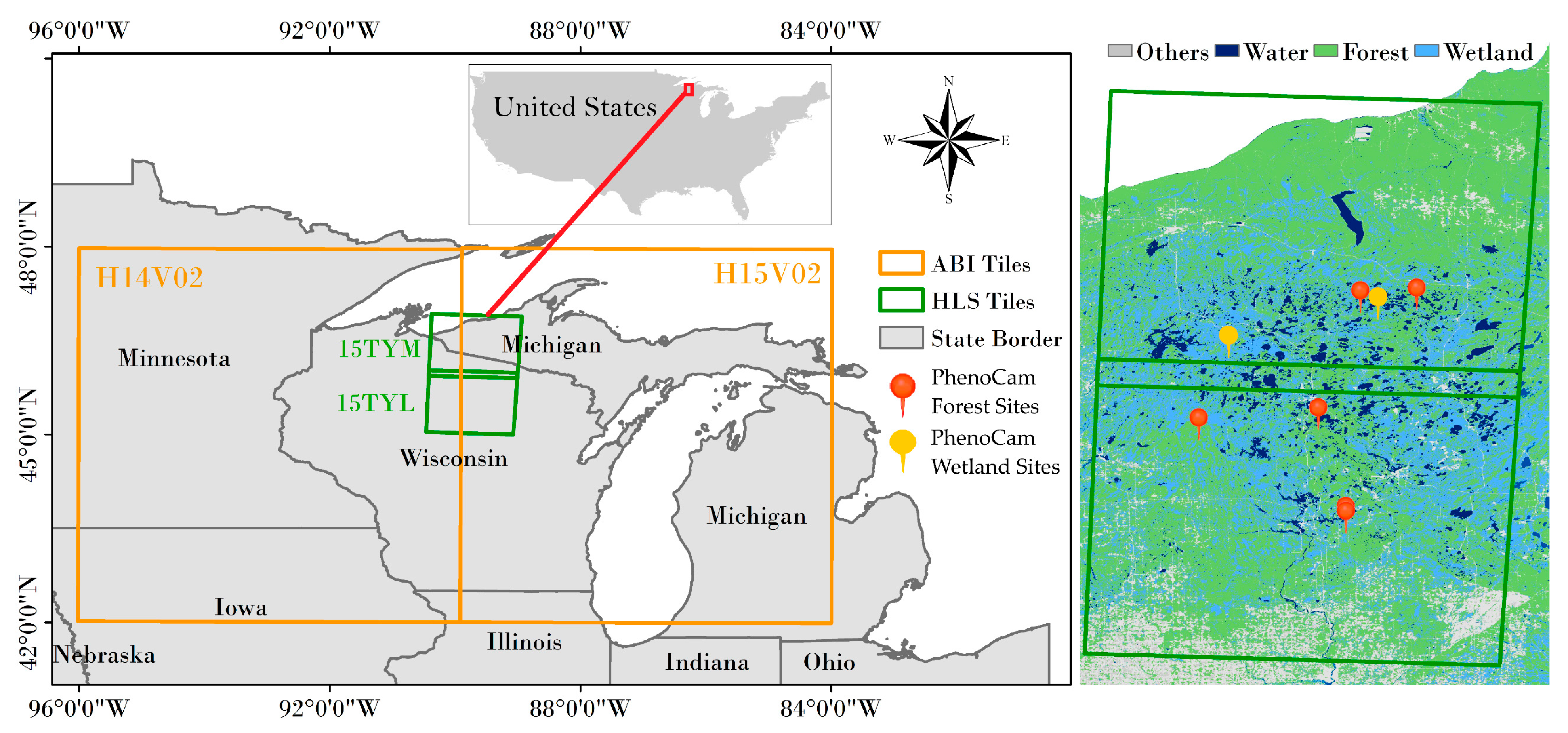
2.1. Study Area and Data

We focused on an area located around the northern Michigan and Wisconsin states (Figure 1), where typical rainy and cloudy weather happened frequently in early growing season [18,25]. In this area, there are only about two-three months on average each year without cloud cover (http://climexp.knmi.nl/ accessed on 1 November 2021). Optical satellite observations in winter and early spring season are commonly contaminated by clouds and snow, which significantly influence land surface monitoring.

2.1.1. Land Cover Data

Land cover type was extracted from the cropland data layer (CDL) produced by the National Agricultural Statistics Service (NASS) of the US Department of Agriculture (USDA). This product has a spatial resolution of 30 m covering the entire Continuous US (CONUS) [44]. Based on the CDL in 2018, we identified locations of forest, wetland, and all vegetation types (“all”) for further extracting corresponding onsets of greenup and senescence dates. In the research area, the proportion of different land cover types was showed below (

Table 1. The proportion of land cover types in the study area.

Land Cover	Proportion	Details
Forest	52%	deciduous forest (47%), evergreen forest (2%), mixed forest (3%)
Wetland	14%	woody wetland (8%) and herbaceous wetland (6%)
Water	7%	open water (7%)
Others	27%	developed (25%), and a small area of croplands (<2%)

).

2.1.2. HLS NBAR Data

The HLS V1.4 dataset provides radiometrically “harmonized’ time series of surface reflectance images, which currently covers the entire North American area and a few selected tiles in other regions of the world. The integration of both Operational Land Imager (OLI) instrument onboard Landsat 8 and the Multi-Spectral Instrument (MSI) onboard Sentinel-2 is able to observe the ground at a field-scale (30 m) ~3 days varying with latitude [27]. To generate HLS data, a set of process is applied to both Landsat-8 and Sentinel-2 images, including consistent atmospheric correction [45], cloud screening and snow detection [46], spatial co-registration and gridding [47], surface reflectance adjustment using nadir bidirectional reflectance distribution function (BRDF) (NBAR) [48,49], and spectral bandpass across sensors [26]. HLS imagery has a tile-dimension of ~110 km (3660 by 3660 pixels) with the projection of the UTM-based Military Grid References System (MGRS- https://hls.gsfc.nasa.gov/products-description/tiling-system/accessed on 19 September 2018) and is available since 2013 (https://hls.gsfc.nasa.gov/data/v1.4/accessed on 2 January 2021). The quality assurance (QA) flags are also included in HLS product, such as snow/ice, clouds, cloud shadows, and water. In this study, two tiles time series of HLS NBAR product (Figure 1. 15TYM and 15TYL) from 1 January 2018 to 31 December 2018 were acquired to produce high-quality time series EVI2 (two-band enhanced vegetation index) [50]. The EVI2 has two main advantages: (1) less sensitive to bare ground cover and higher sensitive to denser vegetation canopy than Normalized Difference Vegetation Index (NDVI) [51,52], and (2) no requirement of blue band, which could improve the applicability of EVI in spectroradiometers without blue bands [50]. The EVI2 was calculated using equation 1. Note that the high-quality HLS time series means the clouds and snow related abiotic contaminations are removed based on the QA flags.

$$\mathrm{EVI}2=\mathrm{G} \left(\frac{{\rho }_{Nir}-{\rho }_{red}}{{\rho }_{Nir}+C\ast {\rho }_{red}+L}\right)$$

(1)

where ${\rho }_{Nir}$ and ${\rho }_{red}$ are spectral reflectance in the near-infrared and red bands, respectively; L (=1), C (=2.4), and G (=2.5) are scaling factors for canopy background adjustment, aerosol resistance coefficient, and a gain factor.

2.1.3. GOES-16 ABI Data

The Top-of-Atmosphere (TOA) reflectance is one of the GOES-16 ABI products generated by Geostationary-NASA Earth Exchange (GeoNEX) project [42], in which the Bidirectional Reflectance Factor (BRF) for Bands 1–6 are provided. This dataset is distributed by a commonly defined tile-gridding in the geographic (latitude/longitude) projection, which is chosen to facilitate intercomparisons between geostationary and polar-orbiting sensors [53]. This gridding system starts from upper-left corner at (60°N, 180°W) to lower-right corner (60°S, 180°E), in which the grid is divided into 6° × 6° tiles that are labelled 0–59 in the horizontal direction and 0–19 in the vertical direction. The pixels in this product are produced into a nadir 500 m spatial resolution for red band (band-2) and 1 km spatial resolution for near-infrared band (band-3). Note that (1) the 1 km near-infrared and short-wave infrared bands are both resampled using nearest neighbor algorithm to create compatible 500 m resolution images with native red band, and (2) the ABI TOA data for 2018 has 15 minutes revisit frequency while it is 10 min in 2019 because of the scan model changed. The ABI TOA product is available from 1 January 2018 to present at https://data.nas.nasa.gov/geonex/data.php?dir=/geonexdata/ accessed on 27 May 2021. In this study, we downloaded two tiles (Figure 1. h15v02 and h14v02) of time series ABI TOA product since 1 January 2018 to 31 December 2018.

2.1.4. Time Series of PhenoCam Data

The PhenoCam network provides near-surface canopy phenology across hundreds of sites distributed in various ecosystems of the United States and some parts of the world. With its high spatial (single vegetation type to the whole canopy) and temporal resolution (every half-hour), the canopy greenness indices derived from PhenoCam photographs have become a robust tool to evaluate the satellite based LSP [54,55]. Unlike conventional remote sensing, PhenoCam provides imagery that is continuous in time, free of contamination by clouds and reasonably built a bridge between ground monitoring by human observers and satellite based LSP detections due to its ability to capture the phenological signal of either the individual organisms (i.e., specific tree/crop type) or the whole canopy (landscape) [56]. The time series of PhenoCam images are freely available from http://klima.sr.unh.edu/accessed on 5 November 2021. In this study, the time series images of 7 PhenoCam sites, including five deciduous broadleaf (DB) and two wetland (WL) sites (one was excluded because of no observations in 2018), from 1 January 2018 to 31 December 2018 were downloaded. The region of vegetated pixels was extracted by using graphical user interface (GUI) tool from https://phenocam.sr.unh.edu/webcam/tools/accessed on 5 November 2021. The 30-min green chromatic coordinate (GCC) was calculated from digital numbers (DN) of red (R), green (G), and blue (B) color channels attached in PhenoCam photographs:

GCC = G/(R + G + B)

(2)

In a 3-day interval from 1 January 2018 to 31 December 2018, the GCC values at 30 minutes wise for these vegetated pixels were calculated and the 90th percentile approach was applied to choose the representative GCC value. The 3-day composite could decrease the influence of abnormal GCC values and variations due to weather conditions (such as fogs) and illumination geometry [57]. Finally, the 3-day composite GCC time series was utilized to track LSP using the same approach used for HLS-ABI LSP detections (see Section 2.2.3).

2.2. Phenology Detection from HLS, ABI, and HLS-ABI Time Series

2.2.1. Generation of 3-day EVI2 Time Series for HLS and ABI

3-day time series of EVI2 from HLS NBAR product was generated. First, HLS observations were removed if the corresponding QA flags were labeled as cloud or snow, but the remaining HLS data could still contain the impacts from residual snow and cloud, as well as the inaccurate atmospheric correction. Then, the EVI2, normalized difference vegetation index (NDVI) [51] and normalized difference water index (NDWI) [58] were calculated for the days when HLS images were available, otherwise, they were assigned to a fill value (e.g., 32,767). Because NDWI is sensitive to cloud/atmospheric effects and snow related contamination and NDVI could be used to filter out the abnormal high values in the daily EVI2 since the red band is very easily influenced by the cloud/aerosol, which results in either irregular larger or lower red band reflectance [16,58,59,60,61], the EVI2 was further set to fill value if NDWI > NDVI or EVI2 > NDVI [16]. Finally, 3-day composite was aggregated from daily valid EVI2 from January 2018 to December 2018, which represents high quality HLS EVI2 time series. The NDWI is calculated using the Equation (3):

$$\mathrm{NDWI}=\frac{{\rho }_{nir}-{\rho }_{swir}}{{\rho }_{nir}+{\rho }_{swir}}$$

(3)

where ${\rho }_{Nir}$ and ${\rho }_{swir}$ are spectral reflectance in the near-infrared and short-wave near-infrared (SWIR) bands, respectively.

Because there are no QA flags associated with ABI TOA product, we generated relative high-quality 3-day EVI2 time series from ABI data based on the following steps. First, we only acquired the ABI images obtained during 8 am to 5 pm within a 3-day period and removed all the observations if NDWI > NDVI or EVI2 > NDVI in order to reduce the snow and cloud-related noise. Then, we performed the 90th percentile approach to the remaining EVI2 values within a 3-day period to select an observation to represent the 3-day EVI2. Finally, we calculated mean and standard deviation (SD) of EVI2 within a 7-point moving window and filtered out the corresponding EVI2 values that were less than mean-SD because EVI2 contaminated by clouds is always abnormally low. Selecting this window length was optimal based on our tests. Although different lengths could remove more or less outliers, resultant time series remained very similar.

2.2.2. Fusion of EVI2 Time Series between HLS and ABI

A synthetic high spatiotemporal resolution HLS-VIIRS EVI2 time series was reconstructed by fusing HLS and ABI data using a newly developed Spatiotemporal Shape-Matching Model (SSMM) [24,62]. The fundamental assumption for this model is that the temporal shape (phenological behavior) of both fine and coarse resolution time series is closely comparable while their magnitudes may differ largely and phenological phases may shift even for the same and neighboring vegetation species. Therefore, for a given HLS pixel from 1 January 2018 to 31 June 2018 (one year), the HLS EVI2 temporal shape could match with one neighboring ABI EVI2 time series though the seasonality and the spatial coverages of both pixels could be different. Within a 5 km window around a given HLS pixel, the HLS time series was compared to a set of the 500 m ABI time series using the equations 4 and 5 (as following), which was called spatiotemporal matching, to select the most similar ABI EVI2 time series as the reference shape model. This reference shape model was then used to predict the gap observations in the time series of HLS high-quality EVI2 that was obstructed by cloud or no overpasses, resulting in a synthetic 30 m HLS-ABI time series.

$$HLS\left(t\right)=\alpha \times ABI\left(T\right)+\gamma$$

(4)

$$T=\gamma \left(t+\beta \right)$$

(5)

where t is the time in number of days starting from 1st January of the one-year fitting window; $\mathrm{HLS}\left(t\right)$ is high quality EVI2 observations while $\mathrm{ABI}\left(T\right)$ is the selected high-quality ABI observations; and α, β, γ, and λ are scaling factors. The detailed steps to calculate these scaling factors are provided in a previous study [24]. Briefly, λ is set to 1 based on a set of tests because the same growing season length in a given HLS pixel can most likely be found from an ABI pixel within a window of 5 km under the same local weather condition. By assuming that difference of phenological phase between HLS and ABI time series is less than one month in a local area, β is selected from −30 to 30 days with a 3-day interval once the minimum of mean squared deviation (MSD) and largest correlation coefficient (R) between the observed HLS EVI2 and the predicted HLS-ABI EVI2 is obtained from Equation (4).

2.2.3. Phenology Detection from EVI2 Time Series

A Hybrid Piecewise Logistic Model (HPLM) LSP detection (LSPD) algorithm was applied to detect phenological transition dates from the HLS-ABI EVI2 time series. It is because the HPLM-LSPD model directly links functional eigenvalues to biophysical parameters. This model has been successfully applied to generate the phenology product from MODIS and VIIRS data [16,17]. The detail of this algorithm could be found elsewhere [16,60] and here we only briefly outlined it.

After the cloud and snow contaminations in one-year HLS-ABI EVI2 time series were removed in Section 2.2.1 and Section 2.2.2, the Savitzy-Golay filter, the moving averaging and moving median methods were first applied to the EVI2 time series to attenuate irregular variations. Then, the greenup phase and the senescence phase were separated by identifying the slope changes over five-point moving windows in EVI2 time series. By integrating vegetation development under normal and stress conditions, the HPLM was further developed to rebuild the seasonal trajectory of vegetation greenness [63,64]. Finally, the key phenometrics were automatically identified by detecting the local extremes of curvature change rate in the HPLM reconstructed EVI2 time series. Vegetation greenup onset during spring and senescence onset during autumn were retrieved because they are the most important phenological transition dates in a vegetation growth cycle.

2.3. Intercomparisons among Remotely Sensed Greenup and Senescence Onsets

The quality of EVI2 time series was investigated as it is the major source of uncertainty in phenology detections [36]. The number of cloud-free 3-day EVI2 composite from HLS and ABI during spring (Astronomical spring from 20th March to 20th June, DOY from 79 to 171 in 2018) was counted and the related pixel frequency was calculated. Because the HPLM model fitting is highly associated with high-quality observations [16] and the cloudy and rainy weather always happens in this region, particularly in the spring period, the reconstructed EVI2 time series for individual forest and wetland pixels from HLS, ABI, and HLS-EVI2 were also compared.

The greenup and senescence onsets derived from HLS-ABI were evaluated by comparing with the detections from ABI and HLS spatially and statistically over the study area in 2018. First, the overall spatial pattern of greenup and senescence onsets from the three time series were visually examined to reveal their differences. Second, the differences of greenup and senescence onset detections were separately analyzed over forest pixels, wetland pixels, and all vegetated land surfaces. In the comparison process with ABI data, the 30 m HLS or HLS-ABI LSP detections over a specified “pure” land cover pixel were aggregated into 500 m by averaging the 30 m valid LSP dates in a given 500 m pixel.

2.4. Evaluation of HLS-ABI Greenup and Senescence Onsets Using PhenoCam Observations

The start-of-spring (SOS) and start-of-autumn (SOA) derived from PhenoCam GCC time series was used to validate the satellite phenometrics from HLS-ABI, HLS, and ABI respectively. The geometric mean functional regression (GMFR) model [65] was used to quantify the difference of phenological timings between PhenoCam GCC derived LSP in seven sites and satellite LSP separately. This model considers variances from both independent (PhenoCam LSP) and dependent variables (satellite LSP) and their slopes could manifest the uncertainty between the two variables. Besides, the average absolute difference (AAD) and the root mean square difference (RMSD) were used to evaluate the statistical dispersion and bias between near surface phenological observations and satellite phenological detections. AAD measures their statistical dispersion by calculating the average absolute difference, while RMSD could measure the quadratic mean of these differences.

3. Results

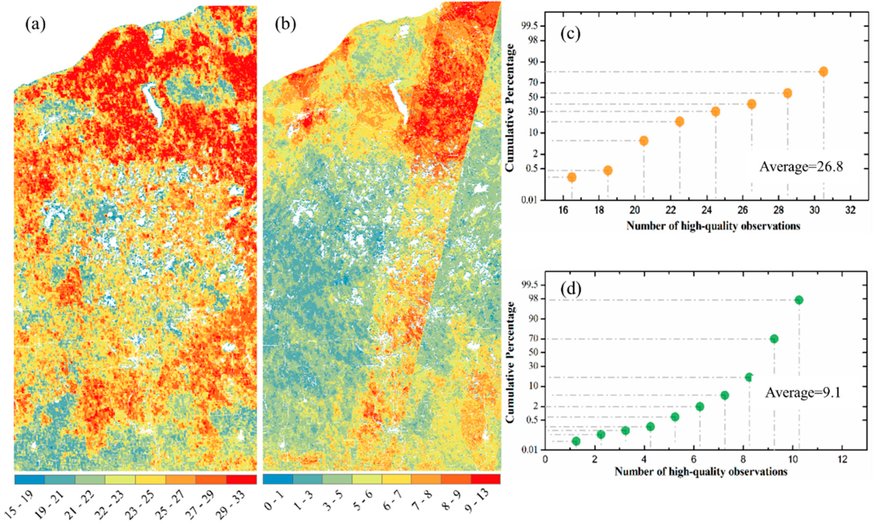
3.1. Differences in the Number of High-Quality Observations in Spring

Figure 2 shows the spatial variation of high-quality observation numbers from HLS and ABI data in astronomical spring (from DOY 79 to 171) in 2018. Overall, the number of high-quality observations for northern forest area was larger than central wetland area either for ABI or HLS data (Figure 2a,b). ABI observations with high-quality increased from 15–19 in southern vegetated lands, to 22–25 in middle wetland, and to 29–33 in northern forest areas (Figure 2a). Differences in HLS observations were apparent around the satellite overpass-orbits (southernwest to northerneast) where pixels within the area could have up to 13 observations while the neighboring pixels only had less than 5 or even 3 observations (Figure 2b). The number of high quality observations in HLS and ABI data varied most in the central wetland area, which was 22–23 on average in ABI data but less than 5 in HLS (Figure 2a,b). In other words, HLS only provided <5 high quality observations for reconstructing the vegetation temporal trajectories in early spring period. The plots of cumulative areal percentage further showed that ABI was able to provide on average 26.8 high quality observations, which was approximately 3 times higher than HLS even in the HLS orbit overlapping area (Figure 2c,d). In addition, high quality observation was less than 10 in more than 90% HLS pixels, while it was more than 20 in over 90% ABI pixels (Figure 2c,d).

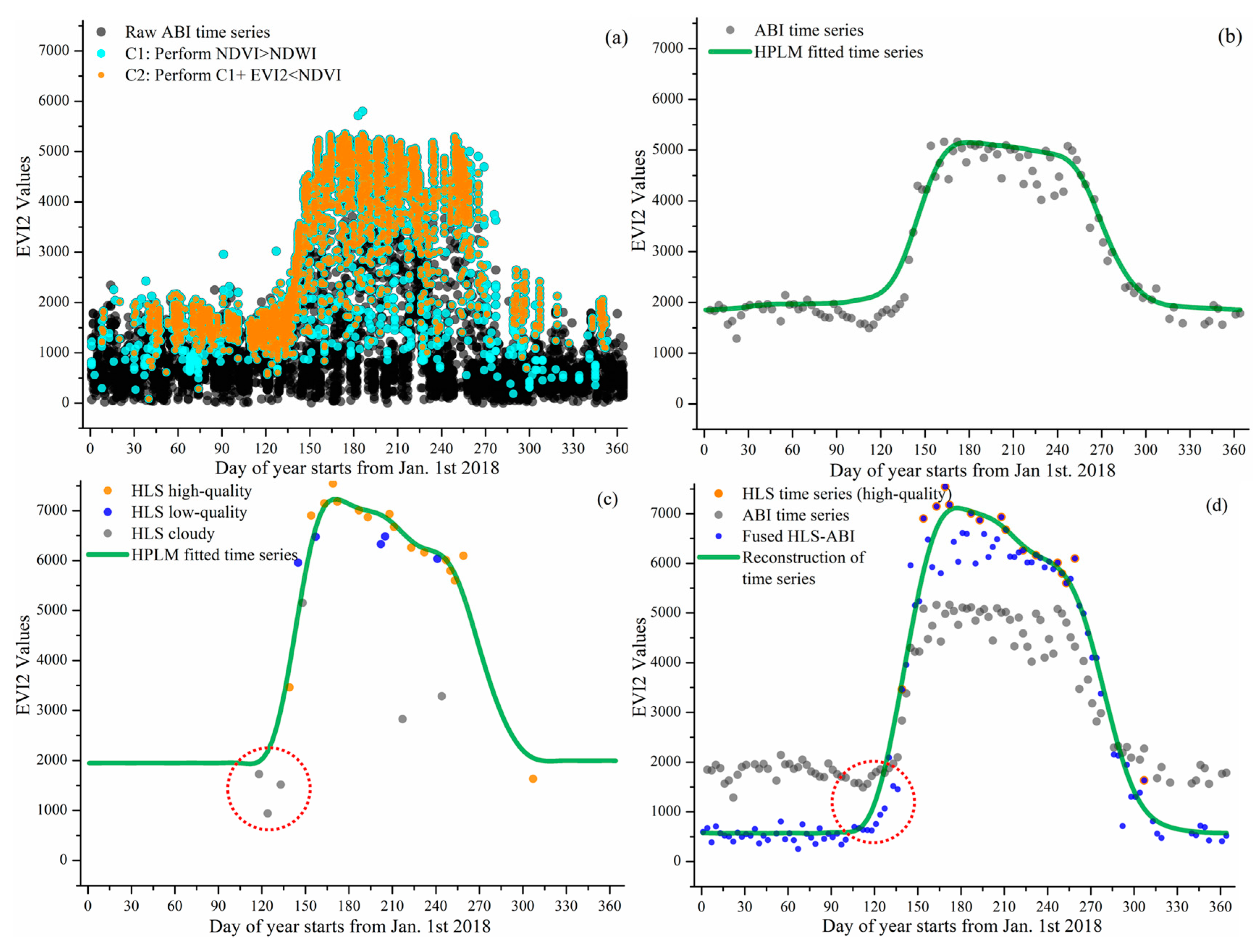
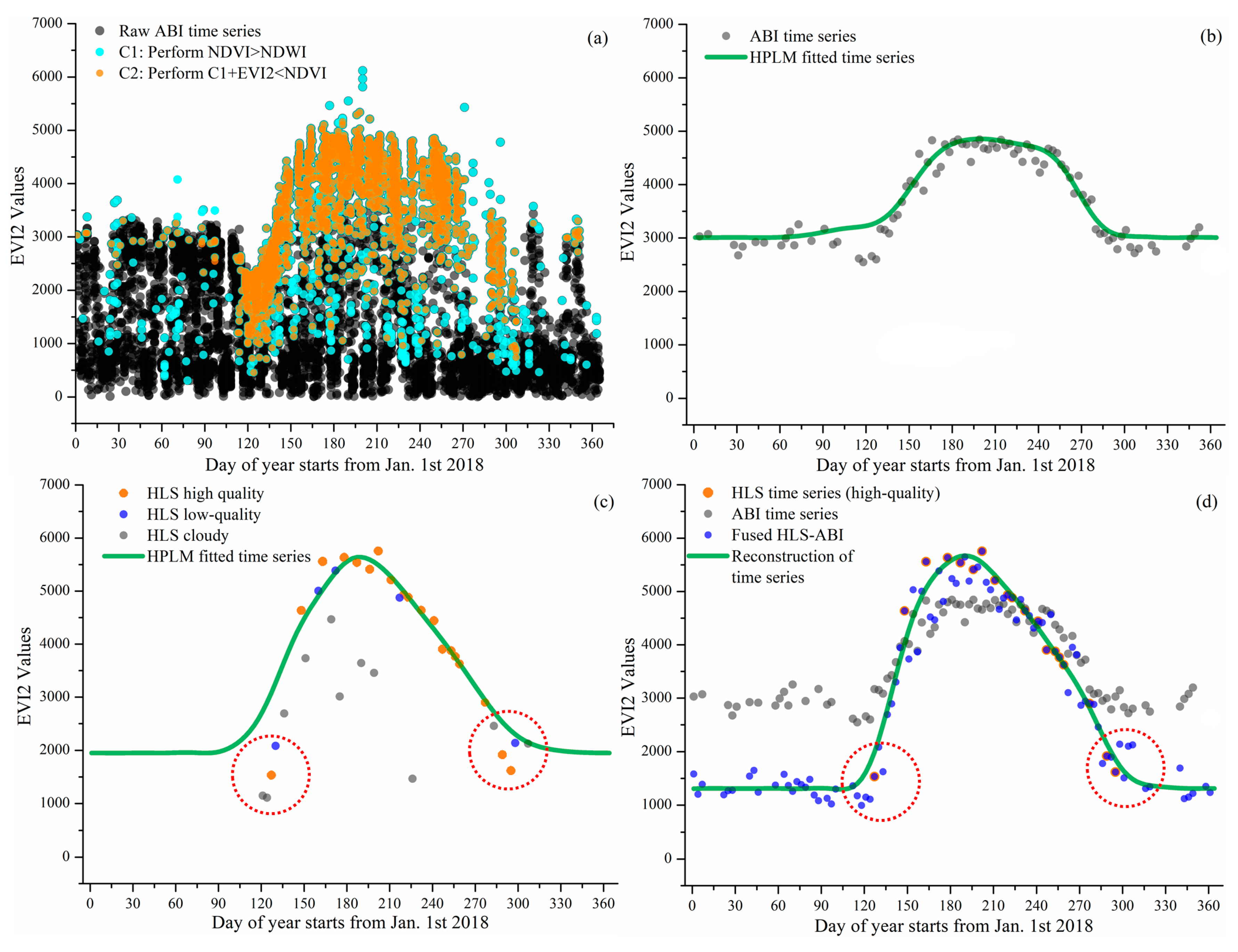
3.2. EVI2 Time Series Reconstruction

Figure 3 and Figure 4 present the reconstruction of EVI2 seasonal trajectories from HLS, ABI, and HLS-ABI in one sample deciduous broadleaf pixel (46°59′12″N, 88°30′36″W) and one sample wetland pixel (46°06′06″N, 90°24′35″W), respectively. Figure 3a and Figure 4a show the noise reduction in 10-15 minutes EVI2 observations. Clearly, a large amount of EVI2 contaminated by snow and cloud were removed using the condition of NDVI > NDWI and the abiotic noise was further reduced by applying the condition of EVI2 < NDVI. Figure 3b and Figure 4b indicate that the resultant 3-day EVI2 time series, by performing 90th percentile in a 3-day interval and a moving window to remove noise in the one-year period, well captured the seasonal variation of forest and wetland plant growth. These temporal ABI EVI2 values were considered as high-quality although some irregular fluctuations existed, which were normal in satellite observations. The ABI seasonal trajectory fitted by HPLM closely tracked the 3-day EVI2 values, which was more reasonable than temporal HLS observations in charactering vegetation phenology development (Figure 3b,c and Figure 4b,c). For the sample forest pixel, there were only one high quality HLS observation during the spring period of 20 March–18 May 2018, and sparse data after 30 August 2018 (Figure 3c). For the sample wetland pixel, only one high-quality HLS observation obtained during 1 Jan 2018 to 10 May of 2018 (Figure 4c).

Figure 3d and Figure 4d show the reconstruction of HLS-ABI EVI2 time series in the sample deciduous forest and wetland pixels, respectively. For the sample forest pixel, around the timing of vegetation greenup onset as denoted in the red circles, HLS EVI2 values were cloud contaminated, which were not used to reconstruct the HLS-ABI time series (Figure 3c), but the temporal shape was well defined in ABI EVI2. For the wetland pixel, around the greenup onset and dormancy onset in 2018, as denoted in the red circles, the high quality HLS observations were not properly used for capturing HLS phenology due to the process of very sparse observations for background determination [64], but they were well utilized in the fusion process for reconstructing HLS-ABI EVI2 time series (Figure 4c,d). Thus, the fused HLS-ABI EVI2 time series was reasonably generated using the SSMM algorithm (Figure 3d and Figure 4d). The magnitude difference of HLS and ABI EVI2 was as large as 0.2 for forest pixel from late spring to early autumn in 2018, while it was smaller for wetland pixel (~0.05) in 2018 spring because of the difference in spatial coverage and reflectance quality (particularly atmospheric effects in ABI data). Due to the insufficient HLS observations, the seasonal shift between HLS and ABI time series for both the forest and wetland pixel was unclear, while the spring and autumn phases of HLS-ABI occurred earlier and later than ABI data, respectively (Figure 3d and Figure 4d). The temporal shape of reconstructed HLS-ABI matched well with HLS high-quality observations and with those predicted using ABI EVI2 during the long-lasting HLS gaps in spring (Figure 3d and Figure 4d). However, the calculated background EVI2 from HLS-ABI differed from ABI and HLS because actual background EVI2 was not available in HLS observations (Figure 3b–d and Figure 4b–d). Note that the calculated background EVI2 in the annual time series represents a mixture of bare soil, green leaves (from evergreen plants), and non-photosynthetic vegetation during vegetation dormancy. The background EVI2 could shift year by year and the calculation could be found in the reference [64].

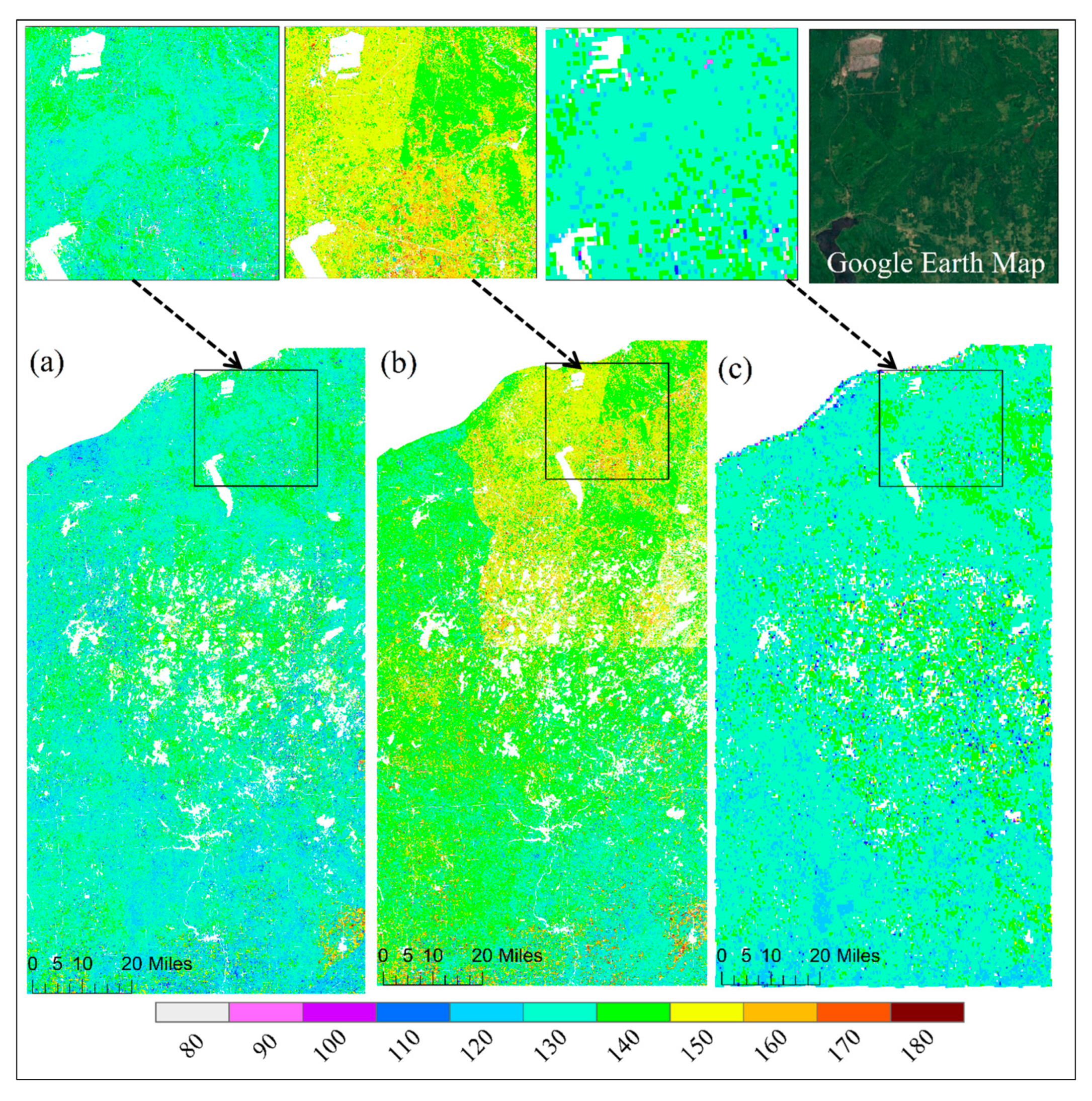
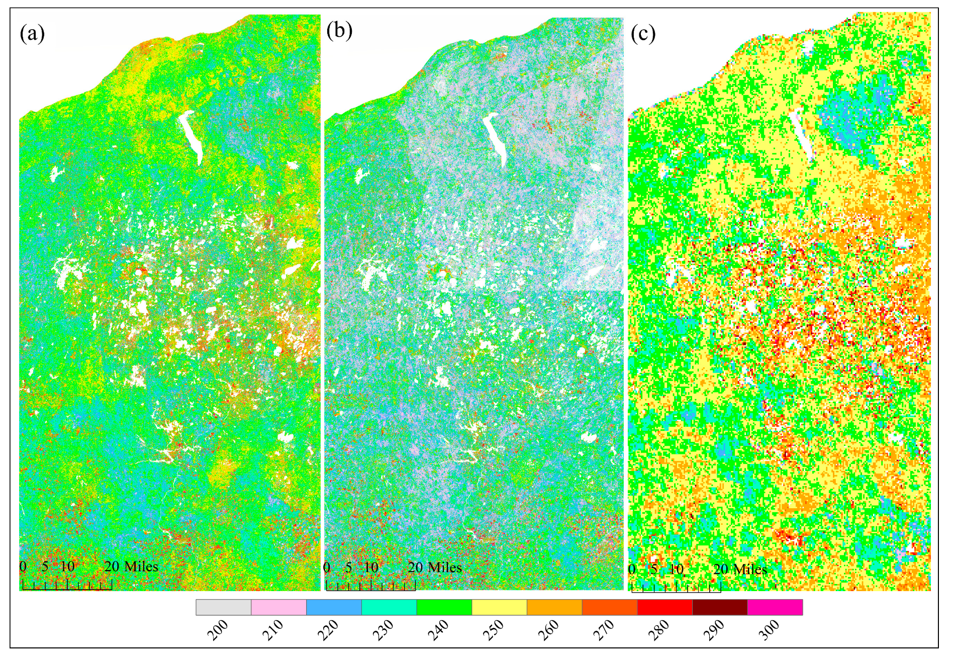
3.3. Spatial Pattern of Greenup and Senescence Onsets

Figure 5 and Figure 6 show the spatial pattern of greenup onset and senescence onset dates over vegetated land surface detected from HLS-ABI, HLS, and ABI data, respectively. The HLS-ABI greenup onset and senescence onset were comparable to the pattern from ABI but overall earlier than those from HLS alone. However, greenup onset and senescence onset in HLS detections exhibited a significant late and early pattern, separately, in the northeast area and a sharp boundary along the edges of adjacent satellite orbits (Figure 5b and Figure 6b). The difference of greenup onset along the orbit overlapping area was as large as 20 days. Such large differences are likely caused by the spatial contrast in available high-quality observations (Figure 2b). Compared to HLS-ABI and HLS detections, ABI greenup and senescence onsets covered a much larger spatial coverages (500–1000 m), resulting in a smoother (coarser) pattern (Figure 5c and Figure 6c). Because of the rich ABI observations, the timing of detected greenup onset was earlier than HLS greenup onset (Figure 5c). In addition, because of the effect of mixture pixels, there were some sparse and isolated lower ABI greenup onset values and higher ABI senescence onset values neighboring to water and around wetlands (Figure 5c and Figure 6c), which were not appeared in HLS-ABI detections. The spatial differences were much clear in the enlarged top panels, which further revealed large uncertainties in HLS detections and lack of spatial detail in ABI detections, while better quality with spatial details in HLS-ABI detections.

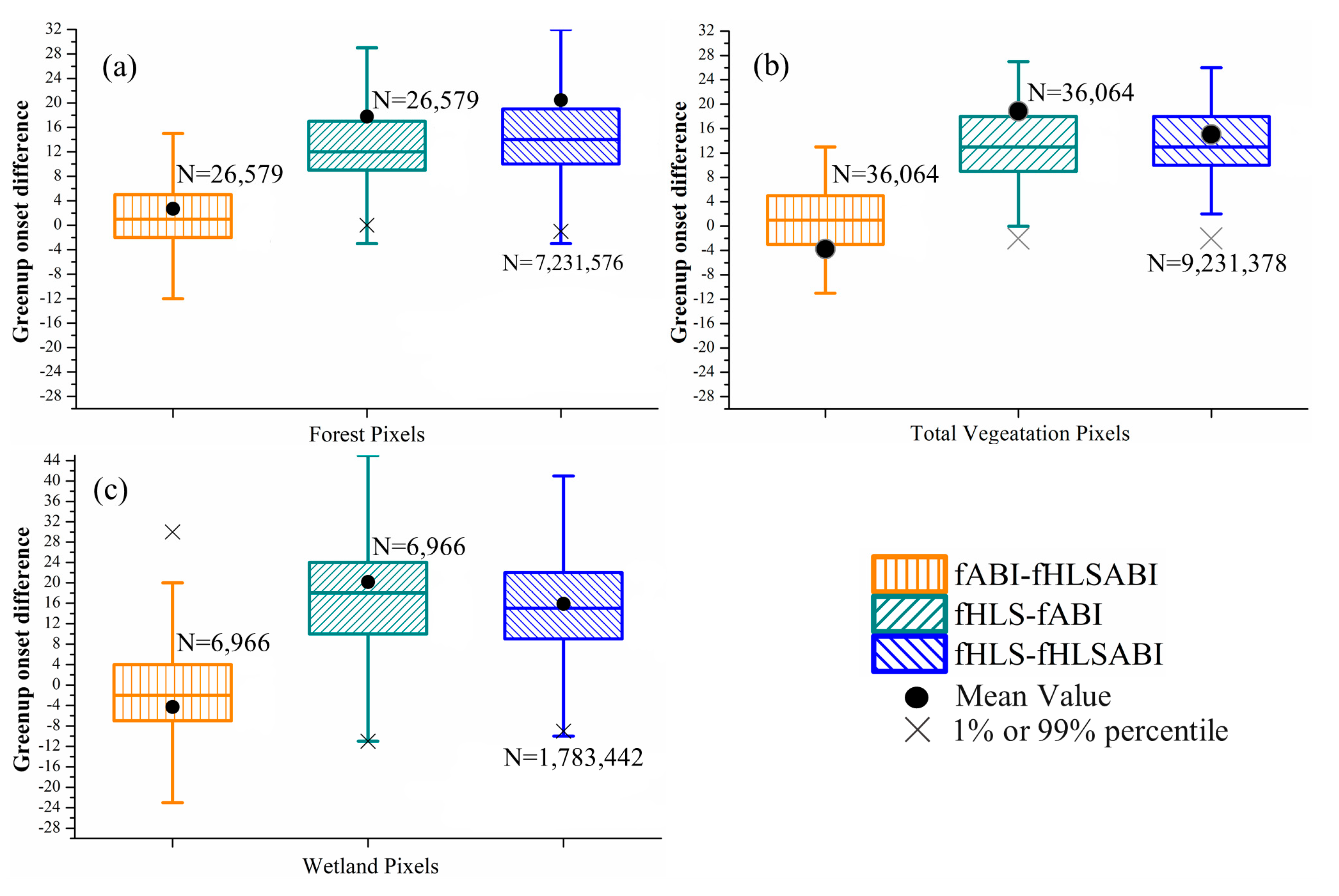
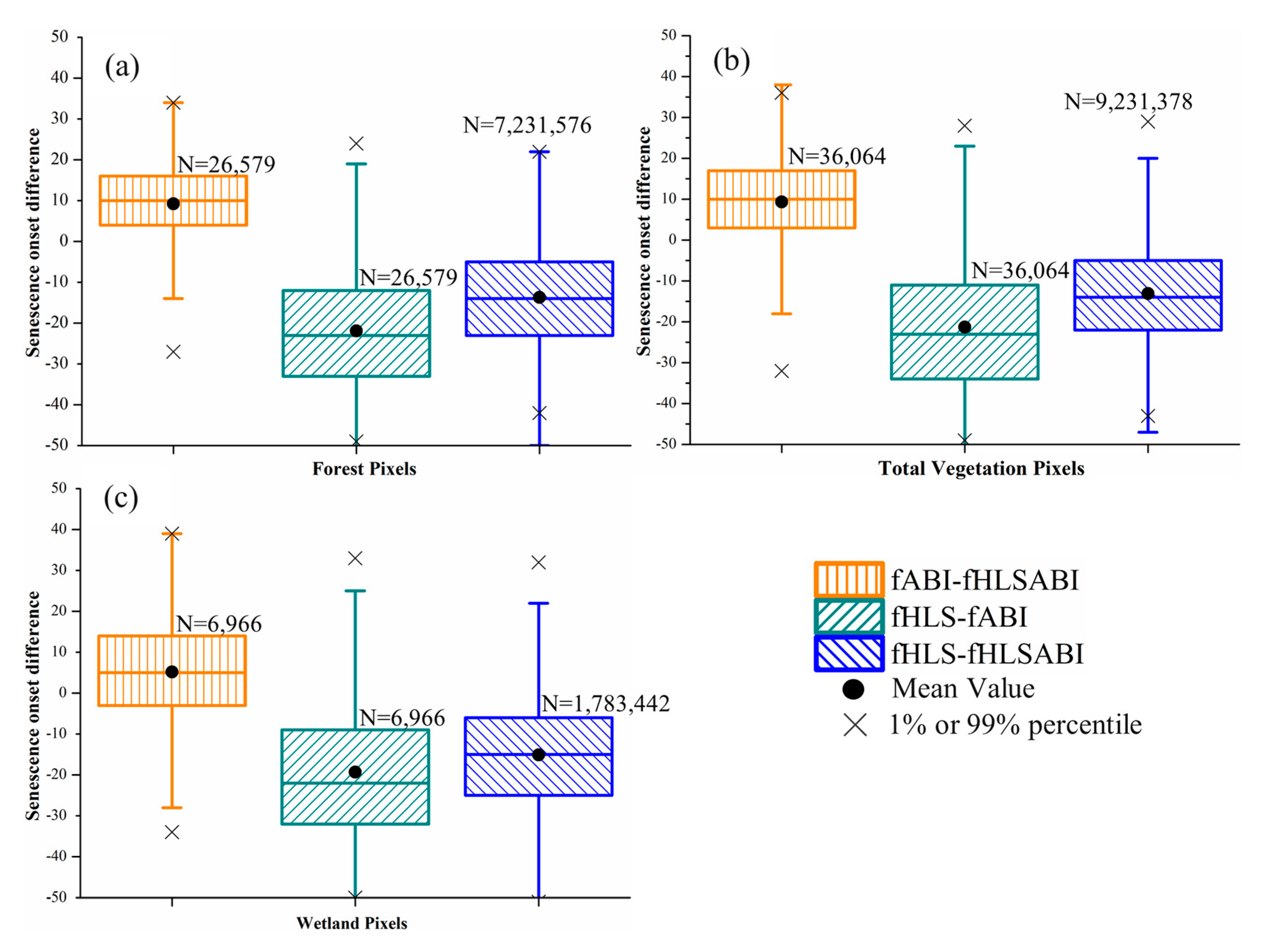
3.4. Intercomparison of Phenology Detections from Different Time Series

Figure 7 and Figure 8 present the intercomparisons of greenup and senescence onsets detected from HLS, ABI, and fused HLS-ABI over pixels from forest, wetlands, and all vegetation types (including forest, wetlands and other vegetation types), separately. For greenup onset detections, ABI showed small bias to HLS-ABI detections over pixels of forest and wetland with a median difference of 1 day earlier and 2 days later, respectively (Figure 7a,c). In addition, the greenup difference between ABI and HLS-ABI detections ranged from −6 to 6 days in more than 50% forest and wetland pixels (Figure 7a,c). The HLS greenup onset, on the other hand, was later in forest and wetland areas with a median difference of 12- and 18-days respectively, in comparison to ABI detections, and with a median difference of 14 and 15 days, respectively, relative to HLS-ABI detections (Figure 7a,c). Moreover, the variation of greenup onset difference was larger in wetland pixels than forest pixels (Figure 7a,c). Considering all vegetated pixels in this area, HLS detections shifted towards later greenup onset relative to both ABI and HLS-ABI detections while there was very small bias between ABI and HLS-ABI detections (Figure 7b). Specifically, the difference of HLS detections with ABI and HLS-ABI detections was 9 to 18 days in more than 50% pixels with a median difference close to 13 days. Compared with HLS-ABI detections, ABI greenup onset showed a median difference of 1 day later and a mean difference of 4 days earlier.

For senescence onset, the difference was distinguishable among the detections from three time series of HLS, ABI, and HLS-ABI (Figure 8). The differences between ABI and HLS-ABI in forest and wetland pixels were similar, with a median value of ~10 days (Figure 8a,b). In all vegetation pixels, however, ABI detections showed a smaller bias (5 days later) relative to HLS-ABI detections (Figure 8c). The HLS detections were earlier than ABI and HLS-ABI with a median difference of ~25 and ~15. days, respectively, in both forest and wetland pixels, and a median difference of 23 and 17 days, respectively, in all vegetation pixels. Overall, the differences in senescence onset among the three times series were larger than those in greenup onset (Figure 7 and Figure 8).

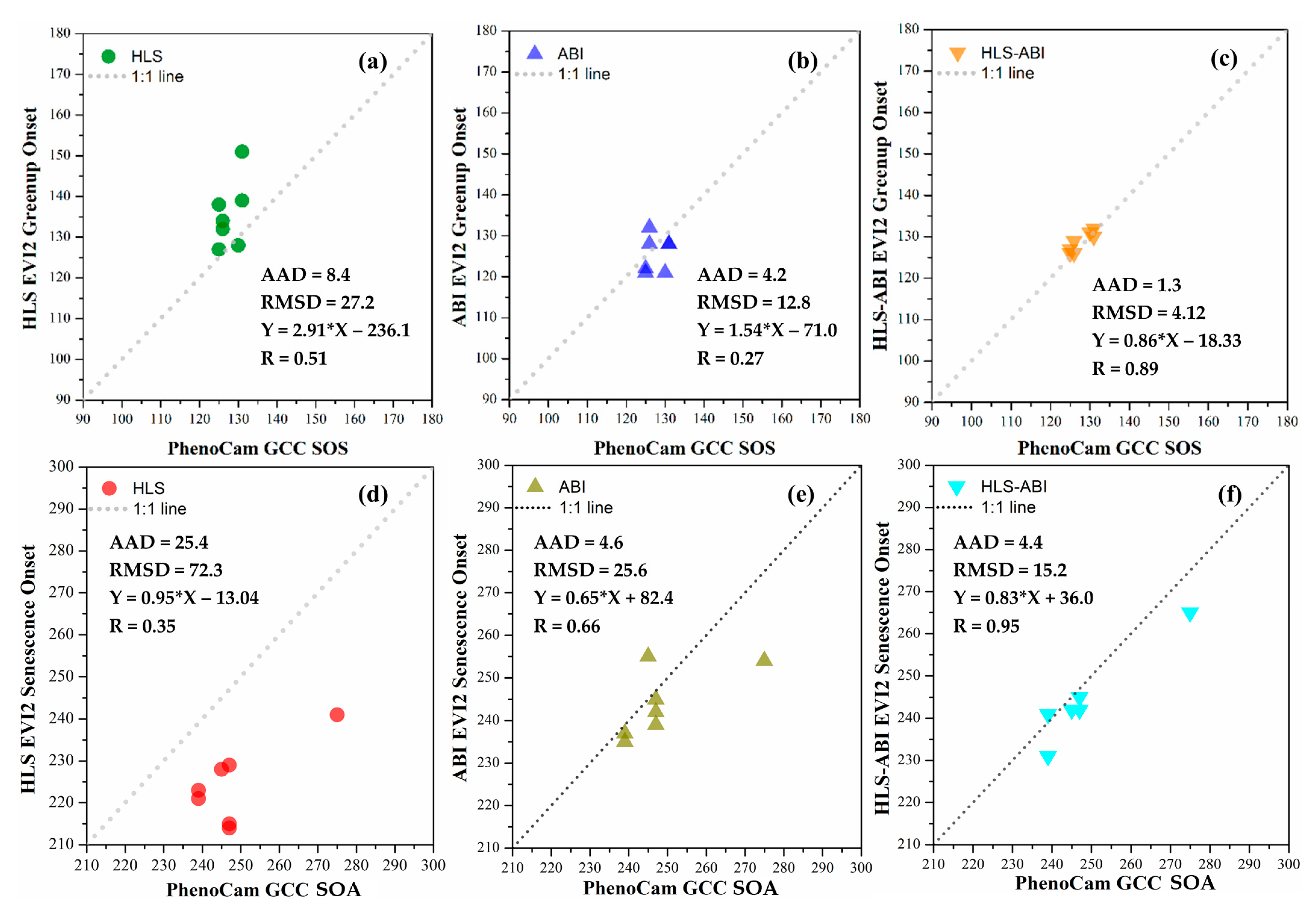
3.5. Evaluation of Satellite Phenology Using PhenoCam Observations

Figure 9 shows the evaluation of greenup onset and senescence onset detections from HLS, ABI, and HLS-ABI using 7 PhenoCam observations including five deciduous broadleaf and two wetland sites in 2018.

For greenup onset, HLS detections were later than PhenoCam SOS with the sample-pairs distributed above the 1:1 line and with an AAD of 8.4 days and RMSD of 27.2 days (Figure 9a). The differences between ABI and PhenoCam detections were 4.2 days in AAD and 12.8 days in RMSD, which were smaller than those between HLS and PhenoCam detections (Figure 9b). HLS-ABI greenup onset, however, had a good agreement with PhenoCam SOS with a slope close to 1.0 and a correlation coefficient (R) of 0.89 (p-value < 0.001) (Figure 9c). It had a small AAD (1.3 days) and RMSD (4.1 days) relative to PhenoCam SOS, suggesting that the greenup detection from HLS or ABI alone was improved by fusing HLS and ABI over this area.

For senescence onset, HLS detections were much earlier than PhenoCam SOA with all the points below the 1:1 line, and their AAD and RMSD were 25.4 and 72.3 days, respectively (Figure 9d). ABI detections showed an AAD of 4.6 days and RMSD of 25.6 days relative to PhenoCam SOA detections, but a better correlation coefficient (R = 0.66) than that between HLS and PhenoCam detections (R = 0.35) (Figure 9e). HLS-ABI senescence onset, on the other hand, aligned well with PhenoCam SOA with 4.4 days in AAD and 15.2 days in RMSD (Figure 9f). Both the slope (0.83) and correlation coefficient (R = 0.95, p-value < 0.001) between senescence onset from HLS-ABI and PhenoCam SOA and correlation coefficient (R = 0.95, p-value < 0.001) further indicated that HLS-ABI detection was more reliable than those from HLS or ABI alone over this region.

4. Discussion

This study is for the first-time to investigate the capability of geostationary satellite observations (GOES ABI) to improve field scale phenology detections by fusing with Landsat-8 and Sentinel-2 time series. The investigation was performed to detect the timing of spring vegetation greenup onset and autumn vegetation senescence onset in 2018 over the north Wisconsin/Michigan area, where polar-orbiting satellite observations are always obstructed by persistent clouds during spring. In contrast, geostationary satellites provides high-frequency observations, which can peek at land surface with more chances in rainy and cloudy seasons [43]. Thus, geostationary satellite observations are particularly useful for characterizing vegetation phenology in seasonally cloud persistent regions.

Observations from geostationary satellites have much higher effectiveness than MODIS data to track the seasonality of vegetation growth and phenology detections [39,40,43,66]. As revealed in the previous studies, cloud contaminations are the major impacts on the quality of EVI2 time series for phenology detections [16,36]. This obstruction was greatly minimized by generating high-quality ABI EVI2 time series, which included the procedure of selecting the time-window of daytime, applying the snow-cover and abiotic filters, performing approaches of 90th percentile in a 3-day period, and removing noise in a moving window. The reconstructed 3-day EVI2 time series was fairly neat with small fluctuations (Figure 3b and Figure 4b), which was able to detect greenup onset and senescence dates with a reasonable accuracy (AAD of <5 days and RMSD <13 days for spring, AAD of <5 days and RMSD ~25 days for autumn) in comparison with PhenoCam observations (Figure 9b,e). This suggests that the method we provided here is promising to establish ABI EVI2 time series for the description of seasonal vegetation greenness trajectory although the magnitude EVI2 values from ABI TOA observations could be attenuated by atmosphere. Of course, the result of phenology detection could be improved if ABI surface reflectance (SR) product with systematic atmospheric correction and bidirectional effect adjustment becomes available.

Field scale LSP has attracted increasing interest for agricultural and forest management because it provides seasonal vegetation development for the same vegetation types or species. Therefore, HLS or Senitinel-2A/B data alone has been increasingly employed to detect phenometrics over various ecosystems, such as croplands [20,67,68], forests [20,24], and grasslands [67,69]. However, the accuracy of phenometrics derived from HLS or Sentinel-2 is relatively low with high uncertainties [24] because of insufficient temporal sampling, particularly in areas with long-lasting cloud and rainfalls [25]. This is evident in this study (Figure 3c and Figure 4c, red circle), where the absence of high-quality observations in HLS time series around greenup onset highly influenced the determination of background EVI2 and further shifted the detected greenup onset date being later. This limitation has further verified in this study that the number of high-quality observations during spring rainy season was very limited (Figure 2b), and the HLS data alone could cause sharp artificial boundaries in the spatial pattern of high-quality observation numbers (Figure 2b) and phenological detections (Figure 5b and Figure 6b) due to the overlap of different satellite orbits of Landsat and Sentinel-2 in the HLS product. As a result, the HLS derived greenup onset was of a high uncertainty, with a RMSD of >27 days and an AAD of 8.4 days over the forest and wetland areas relative to PhenoCam observations (Figure 9a). This also happened to the HLS derived senescence onset with a RMSD of >72 days and an AAD of 25 days (Figure 9d). Such high uncertainties are similar to other HLS phenology detections that showed a difference of 2–4 weeks over deciduous broadleaf, evergreen needleleaf and wetlands in comparison with PhenoCam detections [20].

The reconstructed HLS-ABI EVI2 time series outperforms EVI2 time series separately generated from HLS and ABI. Relative to HLS, the HLS-ABI took the advantages of dense observations in ABI that significantly minimized the effect of cloudy contaminations and greatly reduced the uncertainties in phenological timings. Further, the HLS-ABI EVI2 time series presented smaller irregular temporal variations and largely increased the spatial details than the ABI time series because all the high-quality HLS observations were used to adjust the temporal shape of HLS-ABI. As a result, the HLS-ABI was able to successfully detect phenometrics in isolated islands surrounded by water and small vegetation areas in urban areas. This result was contrasted to the ABI detections that contained mixed information from both vegetation and adjacent water bodies or neighboring buildings, such as the earlier greenup onset and later senescence onset sparsely distributed around water regions in ABI (Figure 5c and Figure 6c). Comparison with PhenoCam observations also demonstrated that HLS-ABI could provide best agreement (Figure 9).

The SSMM algorithm has been demonstrated, in this study, its capacity and strength in establishing synthetic high spatiotemporal resolution time series from ABI and HLS observations. Unlike STARFM and STARFM-like methods [29,30,31,32], the SSMM algorithm does not require the magnitudes of greenness values in fine and coarse resolution observations to be equivalent. This is particularly important in fusing HLS and ABI-TOA time series because the EVI2 values in these two data are not directly comparable. In the fusion process, the SSMM used the advantages of HLS in high quality 30 m EVI2 values and the benefits of ABI in high quality temporal shape. It should be noted that ABI EVI2 is able to characterize well the temporal shape of vegetation greenness development although the magnitude value could be weakened by the atmosphere. This study also supports the wide applicability of SSMM algorithm that is able to handle the various responses of vegetation to complex environments including phenological timing shifts and greenness magnitude discrepancy between fine and coarse spatial resolution pixels [24].

It should be noted that datasets covering various ecosystems, wide geographical regions, and multiple years are needed to better understand the advantages of HLS-ABI time series for phenology detection. This study only conducted the comparison of phenology detections from HLS-ABI, HLS, and ABI time series in one year and two HLS tiles in the northern Michigan and Wisconsin states, and the evaluation of 7 PhenoCam sites. As a result, the conclusion is not necessarily able to represent various complex ecoregions.

5. Conclusions

This study improved 30 m land surface phenology detections by fusing HLS data with the temporal shape of geostationary satellite data over regions with persistent cloud cover using a robust LSP detection approach. This method establishes high quality ABI EVI2 time series from 10–15 min observations, generates synthetic high spatiotemporal resolution EVI2 time series from HLS and ABI EVI2 time series using SSMM algorithm, and detects greenup and senescence onsets using the HPLM approach. The resultant HLS-ABI greenup and senescence onsets in this study successfully avoided the strip effects in HLS and irregular small ABI LSP detections around water/wetlands and revealed a spatially improved pattern of greenup and senescence onsets at 30 m resolution. The consistency of HLS-ABI greenup and senescence onsets with PhenoCam observations further indicated that the reliability and effectiveness of the proposed algorithm for monitoring 30 m vegetation dynamics over regions where polar-orbiting satellite phenological detections are restricted by cloud impacts.

References

1. Visser, M.E.; Both, C. Shifts in phenology due to global climate change: The need for a yardstick. Proc. R. Soc. B Biol. Sci. 2005, 272, 2561–2569. [Google Scholar] [CrossRef]
2. Wolkovich, E.M.; Cook, B.I.; Allen, J.M.; Crimmins, T.M.; Betancourt, J.L.; Travers, S.E.; Pau, S.; Regetz, J.; Davies, T.J.; Kraft, N.J.B.; et al. Warming experiments underpredict plant phenological responses to climate change. Nature 2012, 485, 494–497. [Google Scholar] [CrossRef] [PubMed]
3. Gray, J.M.; Frolking, S.; Kort, E.A.; Ray, D.K.; Kucharik, C.J.; Ramankutty, N.; Friedl, M.A. Direct human influence on atmospheric CO2 seasonality from increased cropland productivity. Nature 2014, 515, 398–401. [Google Scholar] [CrossRef] [PubMed]
4. Laskin, D.N.; McDermid, G.J.; Nielsen, S.E.; Marshall, S.J.; Roberts, D.R.; Montaghi, A. Advances in phenology are conserved across scale in present and future climates. Nat. Clim. Chang. 2019, 9, 419–425. [Google Scholar] [CrossRef]
5. Richardson, A.D.; Braswell, B.H.; Hollinger, D.Y.; Jenkins, J.P.; Ollinger, S.V. Near-surface remote sensing of spatial and temporal variation in canopy phenology. Ecol. Appl. 2009, 19, 1417–1428. [Google Scholar] [CrossRef] [PubMed]
6. Wu, C.; Wang, J.; Ciais, P.; Peñuelas, J.; Zhang, X.; Sonnentag, O.; Tian, F.; Wang, X.; Wang, H.; Liu, R.; et al. Widespread decline in winds delayed autumn foliar senescence over high latitudes. Proc. Natl. Acad. Sci. USA 2021, 118, e2015821118. [Google Scholar] [CrossRef] [PubMed]
7. Caparros-Santiago, J.A.; Rodriguez-Galiano, V.; Dash, J. Land surface phenology as indicator of global terrestrial ecosystem dynamics: A systematic review. ISPRS J. Photogramm. Remote Sens. 2021, 171, 330–347. [Google Scholar] [CrossRef]
8. Dash, J.; Ogutu, B.O. Recent advances in space-borne optical remote sensing systems for monitoring global terrestrial ecosystems. Prog. Phys. Geogr. Earth Environ. 2016, 40, 322–351. [Google Scholar] [CrossRef]
9. Ahl, D.E.; Gower, S.T.; Burrows, S.N.; Shabanov, N.V.; Myneni, R.B.; Knyazikhin, Y. Monitoring spring canopy phenology of a deciduous broadleaf forest using MODIS. Remote Sens. Environ. 2006, 104, 88–95. [Google Scholar] [CrossRef] [Green Version]
10. Liu, L.; Zhang, X.; Yu, Y.; Gao, F.; Yang, Z. Real-Time Monitoring of Crop Phenology in the Midwestern United States Using VIIRS Observations. Remote Sens. 2018, 10, 1540. [Google Scholar] [CrossRef] [Green Version]
11. Walker, J.J.; de Beurs, K.M.; Henebry, G.M. Land surface phenology along urban to rural gradients in the U.S. Great Plains. Remote Sens. Environ. 2015, 165, 42–52. [Google Scholar] [CrossRef]
12. Liu, L.; Zhang, X.; Yu, Y.; Guo, W. Real-time and short-term predictions of spring phenology in North America from VIIRS data. Remote Sens. Environ. 2017, 194, 89–99. [Google Scholar] [CrossRef]
13. Luo, Z.; Yu, S. Spatiotemporal Variability of Land Surface Phenology in China from 2001–2014. Remote Sens. 2017, 9, 65. [Google Scholar] [CrossRef] [Green Version]
14. Adole, T.; Dash, J.; Atkinson, P.M. Characterising the land surface phenology of Africa using 500 m MODIS EVI. Appl. Geogr. 2018, 90, 187–199. [Google Scholar] [CrossRef] [Green Version]
15. Atzberger, C.; Klisch, A.; Mattiuzzi, M.; Vuolo, F. Phenological Metrics Derived over the European Continent from NDVI3g Data and MODIS Time Series. Remote Sens. 2013, 6, 257–284. [Google Scholar] [CrossRef] [Green Version]
16. Zhang, X.; Liu, L.; Liu, Y.; Jayavelu, S.; Wang, J.; Moon, M.; Henebry, G.M.; Friedl, M.A.; Schaaf, C.B. Generation and evaluation of the VIIRS land surface phenology product. Remote Sens. Environ. 2018, 216, 212–229. [Google Scholar] [CrossRef]
17. Ganguly, S.; Friedl, M.A.; Tan, B.; Zhang, X.; Verma, M. Land surface phenology from MODIS: Characterization of the Collection 5 global land cover dynamics product. Remote Sens. Environ. 2010, 114, 1805–1816. [Google Scholar] [CrossRef] [Green Version]
18. Shen, Y.; Zhang, X.; Yang, Z. Mapping Crop Phenological Metrics at Field Scales by Fusing Time Series of VIIRS and HLS over the United States Corn Belt. In Proceedings of the American Geophysical Union Fall Meeting, San Francisco, CA, USA, 1–17 December 2020; p. GC023-0008. [Google Scholar]
19. Zhang, X.; Wang, J.; Gao, F.; Liu, Y.; Schaaf, C.; Friedl, M.; Yu, Y.; Jayavelu, S.; Gray, J.; Liu, L.; et al. Exploration of scaling effects on coarse resolution land surface phenology. Remote Sens. Environ. 2017, 190, 318–330. [Google Scholar] [CrossRef] [Green Version]
20. Bolton, D.K.; Gray, J.M.; Melaas, E.K.; Moon, M.; Eklundh, L.; Friedl, M.A. Continental-scale land surface phenology from harmonized Landsat 8 and Sentinel-2 imagery. Remote Sens. Environ. 2020, 240, 111685. [Google Scholar] [CrossRef]
21. Gao, X.; Gray, J.M.; Reich, B.J. Long-term, medium spatial resolution annual land surface phenology with a Bayesian hierarchical model. Remote Sens. Environ. 2021, 261, 112484. [Google Scholar] [CrossRef]
22. Liao, C.; Wang, J.; Dong, T.; Shang, J.; Liu, J.; Song, Y. Using spatio-temporal fusion of Landsat-8 and MODIS data to derive phenology, biomass and yield estimates for corn and soybean. Sci Total Environ. 2019, 650, 1707–1721. [Google Scholar] [CrossRef] [PubMed]
23. Vrieling, A.; Meroni, M.; Darvishzadeh, R.; Skidmore, A.K.; Wang, T.; Zurita-Milla, R.; Oosterbeek, K.; O’Connor, B.; Paganini, M. Vegetation phenology from Sentinel-2 and field cameras for a Dutch barrier island. Remote Sens. Environ. 2018, 215, 517–529. [Google Scholar] [CrossRef]
24. Zhang, X.; Wang, J.; Henebry, G.M.; Gao, F. Development and evaluation of a new algorithm for detecting 30 m land surface phenology from VIIRS and HLS time series. ISPRS J. Photogramm. Remote Sens. 2020, 161, 37–51. [Google Scholar] [CrossRef]
25. Gao, F.; Anderson, M.C.; Zhang, X.; Yang, Z.; Alfieri, J.G.; Kustas, W.P.; Mueller, R.; Johnson, D.M.; Prueger, J.H. Toward mapping crop progress at field scales through fusion of Landsat and MODIS imagery. Remote Sens. Environ. 2017, 188, 9–25. [Google Scholar] [CrossRef] [Green Version]
26. Claverie, M.; Ju, J.; Masek, J.G.; Dungan, J.L.; Vermote, E.F.; Roger, J.-C.; Skakun, S.V.; Justice, C. The Harmonized Landsat and Sentinel-2 surface reflectance data set. Remote Sens. Environ. 2018, 219, 145–161. [Google Scholar] [CrossRef]
27. Li, J.; Roy, D.P. A Global Analysis of Sentinel-2A, Sentinel-2B and Landsat-8 Data Revisit Intervals and Implications for Terrestrial Monitoring. Remote Sens. 2017, 9, 902. [Google Scholar] [CrossRef] [Green Version]
28. Fensholt, R.; Sandholt, I.; Stisen, S.; Tucker, C. Analysing NDVI for the African continent using the geostationary meteosat second generation SEVIRI sensor. Remote Sens. Environ. 2006, 101, 212–229. [Google Scholar] [CrossRef]
29. Feng, G.; Masek, J.; Schwaller, M.; Hall, F. On the blending of the Landsat and MODIS surface reflectance: Predicting daily Landsat surface reflectance. IEEE Trans. Geosci. Remote Sens. 2006, 44, 2207–2218. [Google Scholar] [CrossRef]
30. Gao, F.; Hilker, T.; Zhu, X.; Anderson, M.; Masek, J.; Wang, P.; Yang, Y. Fusing Landsat and MODIS Data for Vegetation Monitoring. IEEE Geosci. Remote Sens. Mag. 2015, 3, 47–60. [Google Scholar] [CrossRef]
31. Hilker, T.; Wulder, M.A.; Coops, N.C.; Seitz, N.; White, J.C.; Gao, F.; Masek, J.G.; Stenhouse, G. Generation of dense time series synthetic Landsat data through data blending with MODIS using a spatial and temporal adaptive reflectance fusion model. Remote Sens. Environ. 2009, 113, 1988–1999. [Google Scholar] [CrossRef]
32. Hilker, T.; Wulder, M.A.; Coops, N.C.; Linke, J.; McDermid, G.; Masek, J.G.; Gao, F.; White, J.C. A new data fusion model for high spatial- and temporal-resolution mapping of forest disturbance based on Landsat and MODIS. Remote Sens. Environ. 2009, 113, 1613–1627. [Google Scholar] [CrossRef]
33. Zhu, X.; Chen, J.; Gao, F.; Chen, X.; Masek, J.G. An enhanced spatial and temporal adaptive reflectance fusion model for complex heterogeneous regions. Remote Sens. Environ. 2010, 114, 2610–2623. [Google Scholar] [CrossRef]
34. Zhang, X.; Friedl, M.A.; Schaaf, C.B. Global vegetation phenology from Moderate Resolution Imaging Spectroradiometer (MODIS): Evaluation of global patterns and comparison with in situ measurements. J. Geophys. Res. Biogeosci. 2006, 111. [Google Scholar] [CrossRef]
35. Ju, J.; Roy, D.P. The availability of cloud-free Landsat ETM+ data over the conterminous United States and globally. Remote Sens. Environ. 2008, 112, 1196–1211. [Google Scholar] [CrossRef]
36. Zhang, X.; Friedl, M.A.; Schaaf, C.B. Sensitivity of vegetation phenology detection to the temporal resolution of satellite data. Int. J. Remote Sens. 2009, 30, 2061–2074. [Google Scholar] [CrossRef]
37. Miura, T.; Nagai, S.; Takeuchi, M.; Ichii, K.; Yoshioka, H. Improved Characterisation of Vegetation and Land Surface Seasonal Dynamics in Central Japan with Himawari-8 Hypertemporal Data. Sci. Rep. 2019, 9, 15692. [Google Scholar] [CrossRef] [Green Version]
38. Sobrino, J.A.; Julien, Y.; Sòria, G. Phenology Estimation from Meteosat Second Generation Data. IEEE J. Sel. Top. Appl. Earth Obs. Remote Sens. 2013, 6, 1653–1659. [Google Scholar] [CrossRef]
39. Yan, D.; Zhang, X.; Nagai, S.; Yu, Y.; Akitsu, T.; Nasahara, K.N.; Ide, R.; Maeda, T. Evaluating land surface phenology from the Advanced Himawari Imager using observations from MODIS and the Phenological Eyes Network. Int. J. Appl. Earth Obs. Geoinf. 2019, 79, 71–83. [Google Scholar] [CrossRef]
40. Yan, D.; Zhang, X.; Yu, Y.; Guo, W. A Comparison of Tropical Rainforest Phenology Retrieved from Geostationary (SEVIRI) and Polar-Orbiting (MODIS) Sensors Across the Congo Basin. IEEE Trans. Geosci. Remote Sens. 2016, 54, 4867–4881. [Google Scholar] [CrossRef] [Green Version]
41. Weber, M.; Hao, D.; Asrar, G.; Zhou, Y.; Xuecao, L.; Chen, M. Exploring the Use of DSCOVR/EPIC Satellite Observations to Monitor Vegetation Phenology. Remote Sens. 2020, 12, 2384. [Google Scholar] [CrossRef]
42. Wang, W.; Li, S.; Hashimoto, H.; Takenaka, H.; Higuchi, A.; Kalluri, S.; Nemani, R. An Introduction to the Geostationary-NASA Earth Exchange (GeoNEX) Products: 1. Top-of-Atmosphere Reflectance and Brightness Temperature. Remote Sens. 2020, 12, 1267. [Google Scholar] [CrossRef] [Green Version]
43. Hashimoto, H.; Wang, W.; Dungan, J.L.; Li, S.; Michaelis, A.R.; Takenaka, H.; Higuchi, A.; Myneni, R.B.; Nemani, R.R. New generation geostationary satellite observations support seasonality in greenness of the Amazon evergreen forests. Nat. Commun. 2021, 12, 684. [Google Scholar] [CrossRef] [PubMed]
44. Boryan, C.; Yang, Z.; Mueller, R.; Craig, M. Monitoring US agriculture: The US Department of Agriculture, National Agricultural Statistics Service, Cropland Data Layer Program. Geocarto Int. 2011, 26, 341–358. [Google Scholar] [CrossRef]
45. Vermote, E.; Roger, J.-C.; Franch, B.; Skakun, S. LaSRC (Land Surface Reflectance Code): Overview, application and validation using MODIS, VIIRS, LANDSAT and Sentinel 2 data’s. In Proceedings of the IGARSS 2018—2018 IEEE International Geoscience and Remote Sensing Symposium, Valencia, Spain, 22–27 July 2018; pp. 8173–8176. [Google Scholar]
46. Zhu, Z.; Woodcock, C.E. Automated cloud, cloud shadow, and snow detection in multitemporal Landsat data: An algorithm designed specifically for monitoring land cover change. Remote Sens. Environ. 2014, 152, 217–234. [Google Scholar] [CrossRef]
47. Feng, G.; Jeffrey, G.M.; Robert, E.W. Automated registration and orthorectification package for Landsat and Landsat-like data processing. J. Appl. Remote Sens. 2009, 3, 1–20. [Google Scholar] [CrossRef]
48. Roy, D.P.; Zhang, H.K.; Ju, J.; Gomez-Dans, J.L.; Lewis, P.E.; Schaaf, C.B.; Sun, Q.; Li, J.; Huang, H.; Kovalskyy, V. A general method to normalize Landsat reflectance data to nadir BRDF adjusted reflectance. Remote Sens. Environ. 2016, 176, 255–271. [Google Scholar] [CrossRef] [Green Version]
49. Zhang, H.K.; Roy, D.P.; Kovalskyy, V. Optimal Solar Geometry Definition for Global Long-Term Landsat Time-Series Bidirectional Reflectance Normalization. IEEE Trans. Geosci. Remote Sens. 2016, 54, 1410–1418. [Google Scholar] [CrossRef]
50. Jiang, Z.; Huete, A.R.; Didan, K.; Miura, T. Development of a two-band enhanced vegetation index without a blue band. Remote Sens. Environ. 2008, 112, 3833–3845. [Google Scholar] [CrossRef]
51. Townshend, J.R.G.; Justice, C.O. Analysis of the dynamics of African vegetation using the normalized difference vegetation index. Int. J. Remote Sens. 1986, 7, 1435–1445. [Google Scholar] [CrossRef]
52. Huete, A.; Didan, K.; Miura, T.; Rodriguez, E.P.; Gao, X.; Ferreira, L.G. Overview of the radiometric and biophysical performance of the MODIS vegetation indices. Remote Sens. Environ. 2002, 83, 195–213. [Google Scholar] [CrossRef]
53. Li, S.; Wang, W.; Hashimoto, H.; Xiong, J.; Vandal, T.; Yao, J.; Qian, L.; Ichii, K.; Lyapustin, A.; Wang, Y.; et al. First Provisional Land Surface Reflectance Product from Geostationary Satellite Himawari-8 AHI. Remote Sens. 2019, 11, 2990. [Google Scholar] [CrossRef] [Green Version]
54. Seyednasrollah, B.; Young, A.M.; Hufkens, K.; Milliman, T.; Friedl, M.A.; Frolking, S.; Richardson, A.D. Tracking vegetation phenology across diverse biomes using Version 2.0 of the PhenoCam Dataset. Sci. Data 2019, 6, 222. [Google Scholar] [CrossRef] [PubMed] [Green Version]
55. Zhang, X.; Jayavelu, S.; Liu, L.; Friedl, M.A.; Henebry, G.M.; Liu, Y.; Schaaf, C.B.; Richardson, A.D.; Gray, J. Evaluation of land surface phenology from VIIRS data using time series of PhenoCam imagery. Agric. For. Meteorol. 2018, 256-257, 137–149. [Google Scholar] [CrossRef]
56. Richardson, A.D.; Hufkens, K.; Milliman, T.; Frolking, S. Intercomparison of phenological transition dates derived from the PhenoCam Dataset V1.0 and MODIS satellite remote sensing. Sci. Rep. 2018, 8, 5679. [Google Scholar] [CrossRef] [Green Version]
57. Sonnentag, O.; Hufkens, K.; Teshera-Sterne, C.; Young, A.M.; Friedl, M.; Braswell, B.H.; Milliman, T.; O’Keefe, J.; Richardson, A.D. Digital repeat photography for phenological research in forest ecosystems. Agric. For. Meteorol. 2012, 152, 159–177. [Google Scholar] [CrossRef]
58. Gao, B.-C. NDWI—A normalized difference water index for remote sensing of vegetation liquid water from space. Remote Sens. Environ. 1996, 58, 257–266. [Google Scholar] [CrossRef]
59. Delbart, N.; Kergoat, L.; Le Toan, T.; Lhermitte, J.; Picard, G. Determination of phenological dates in boreal regions using normalized difference water index. Remote Sens. Environ. 2005, 97, 26–38. [Google Scholar] [CrossRef] [Green Version]
60. Gonsamo, A.; Chen, J.M.; Price, D.T.; Kurz, W.A.; Wu, C. Land surface phenology from optical satellite measurement and CO2 eddy covariance technique. J. Geophys. Res. Biogeosci. 2012, 117. [Google Scholar] [CrossRef]
61. Jin, Y.; Schaaf, C.B.; Woodcock, C.E.; Gao, F.; Li, X.; Strahler, A.H.; Lucht, W.; Liang, S. Consistency of MODIS surface bidirectional reflectance distribution function and albedo retrievals: 2. Validation. J. Geophys. Res. Atmos. 2003, 108. [Google Scholar] [CrossRef] [Green Version]
62. Zhang, X.; Gao, F.; Wang, J.; Ye, Y. Evaluating a spatiotemporal shape-matching model for the generation of synthetic high spatiotemporal resolution time series of multiple satellite data. Int. J. Appl. Earth Obs. Geoinf. 2021, 104, 102545. [Google Scholar] [CrossRef]
63. Melaas, E.K.; Friedl, M.A.; Zhu, Z. Detecting interannual variation in deciduous broadleaf forest phenology using Landsat TM/ETM+ data. Remote Sens. Environ. 2013, 132, 176–185. [Google Scholar] [CrossRef]
64. Zhang, X. Reconstruction of a complete global time series of daily vegetation index trajectory from long-term AVHRR data. Remote Sens. Environ. 2015, 156, 457–472. [Google Scholar] [CrossRef]
65. Halfon, E. Regression method in ecotoxicology: A better formulation using the geometric mean functional regression. Environ. Sci. Technol. 1985, 19, 747–749. [Google Scholar] [CrossRef] [PubMed]
66. Wheeler, K.I.; Dietze, M.C. Improving the monitoring of deciduous broadleaf phenology using the Geostationary Operational Environmental Satellite (GOES) 16 and 17. Biogeosciences 2021, 18, 1971–1985. [Google Scholar] [CrossRef]
67. Griffiths, P.; Nendel, C.; Pickert, J.; Hostert, P. Towards national-scale characterization of grassland use intensity from integrated Sentinel-2 and Landsat time series. Remote Sens. Environ. 2020, 238, 111124. [Google Scholar] [CrossRef]
68. Meroni, M.; d’Andrimont, R.; Vrieling, A.; Fasbender, D.; Lemoine, G.; Rembold, F.; Seguini, L.; Verhegghen, A. Comparing land surface phenology of major European crops as derived from SAR and multispectral data of Sentinel-1 and -2. Remote Sens. Environ. 2021, 253, 112232. [Google Scholar] [CrossRef]
69. Gómez-Giráldez, P.J.; Pérez-Palazón, M.J.; Polo, M.J.; González-Dugo, M.P. Monitoring Grass Phenology and Hydrological Dynamics of an Oak–Grass Savanna Ecosystem Using Sentinel-2 and Terrestrial Photography. Remote Sens. 2020, 12, 600. [Google Scholar] [CrossRef] [Green Version]
Figure 1. The study area map. Green rectangle area delineates two Harmonized Landsat Sentinel-2 (HLS) tiles (15TYM and 15TYL), orange rectangle area delineates two Advanced Baseline Imager (ABI) tiles (H14V02 and H15V02) covering both HLS tiles. Right parts show the available 8 PhenoCam sites and the dominated land cover types from 30m Crop Data Layer (CDL) (Section 2.1.1).
Remotesensing 13 04465 g001
Figure 2. Number of high-quality 3-day observations by (a) ABI and (b) HLS data in study area around the greenup onset (astronomical spring from 20th March to 20th June) in 2018. (c,d) show the cumulative areal (or pixel) percentages with ABI and HLS high-quality observation numbers, respectively, calculated from (a,b).
Remotesensing 13 04465 g002
Figure 3. Reconstruction of HLS-ABI time series in a forest pixel. (a) denotes the noise reduction process for selecting high-quality ABI observations from raw ABI observations, where the black dots are the results of overlaps from multiple gray dots. (bd) present the reconstruction of EVI2 temporal trajectories from ABI, HLS, and HLS-ABI, respectively. The value in y-axis is multiplied by 10,000.
Remotesensing 13 04465 g003
Figure 4. Reconstruction of wetland HLS-ABI time series in a wetland pixel. (a) denotes the noise reduction process for selecting high-quality ABI observations from raw ABI observations, where the black dots are the results of overlaps from multiple gray dots. (bd) present the reconstruction of EVI2 temporal trajectories from ABI, HLS, and HLS-ABI, respectively. The value in y-axis is multiplied by 10,000.
Remotesensing 13 04465 g004
Figure 5. Spatial pattern of greenup onset from (a) HLS-ABI, (b) HLS, and (c) ABI data in the study area. Top panels show an enlarged small area from these detections and from the Google Earth Map.
Remotesensing 13 04465 g005
Figure 6. Spatial pattern of senescence onset from (a) HLS-ABI, (b) HLS, and (c) ABI data in the study area.
Remotesensing 13 04465 g006
Figure 7. Boxplots showing the difference of greenup onset detected from three time series in (a) forest pixels, (b) all vegetation pixels, and (c) wetland pixels, respectively. The fABI, fHLS, and fHLSABI represent phenological timings from ABI, HLS, and HLS-ABI data, respectively. Black dots denote the mean difference, while black crosses denote either the %1 or 99% percentile of differences. Black crosses that out of the y-axis range are not displayed. Note that 30 m HLS and HLS-ABI data were aggregated to 500 m for the comparison.
Remotesensing 13 04465 g007
Figure 8. Boxplots showing the difference of senescence onset detected from three time series in (a) forest pixels, (b) all vegetation pixels, (c) wetland pixels, respectively. The fABI, fHLS, and fHLSABI represent phenological timings from ABI, HLS, and HLS-ABI data, respectively. Black dots denote the mean difference, while black crosses denote either the %1 or 99% percentile of differences. Black crosses that out of the y-axis range are not displayed. Note that 30 m HLS and HLS-ABI data were aggregated to 500 m for the comparison.
Remotesensing 13 04465 g008
Figure 9. Comparison of greenup onset and senescence onset detected separately from (a,d) HLS, (b,e) ABI, and (c,f) HLS-ABI with 7 PhenoCam observations.
Remotesensing 13 04465 g009