
Mapping of Coral Reefs with Multispectral Satellites: A Review of Recent Papers

1
Laboratoire de Mathématiques et de Leurs Applications (LMAP), Université de Pau et des Pays de L’adour, E2S UPPA, CNRS, 64600 Anglet, France
2
Department of Mathematics and Statistics, Macquarie University, Sydney, NSW 2109, Australia
3
ARC Centre of Excellence for Mathematical and Statistical Frontiers, School of Mathematical Science, Queensland University of Technology, Brisbane, QLD 4072, Australia
4
Mediterranean Institute of Oceanography (MIO), Université de Toulon, CNRS, IRD, 04120 La Garde, France
5
Mediterranean Institute of Oceanography (MIO), Aix Marseille Université, CNRS, IRD, 04120 La Garde, France
6
Laboratoire des Sciences pour L’ingénieur Appliquées à la Mécanique et au Génie Électrique (SIAME), Université de Pau et des Pays de L’adour, E2S UPPA, 64600 Anglet, France
*
Author to whom correspondence should be addressed.
Remote Sens. 2021, 13(21), 4470; https://0-doi-org.brum.beds.ac.uk/10.3390/rs13214470
Submission received: 20 September 2021
/
Revised: 25 October 2021
/
Accepted: 5 November 2021
/
Published: 7 November 2021
(This article belongs to the Special Issue Computer Vision and Machine Learning for Remote Sensing Solutions Applied to Environmental Challenges)
Abstract
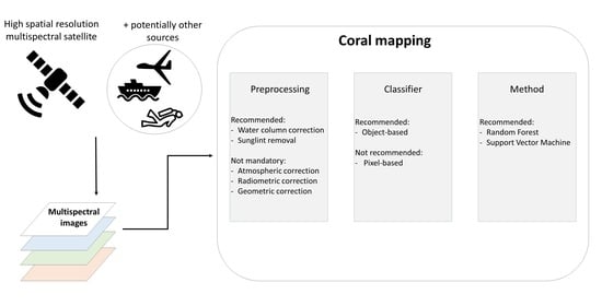
:Coral reefs are an essential source of marine biodiversity, but they are declining at an alarming rate under the combined effects of global change and human pressure. A precise mapping of coral reef habitat with high spatial and time resolutions has become a necessary step for monitoring their health and evolution. This mapping can be achieved remotely thanks to satellite imagery coupled with machine-learning algorithms. In this paper, we review the different satellites used in recent literature, as well as the most common and efficient machine-learning methods. To account for the recent explosion of published research on coral reel mapping, we especially focus on the papers published between 2018 and 2020. Our review study indicates that object-based methods provide more accurate results than pixel-based ones, and that the most accurate methods are Support Vector Machine and Random Forest. We emphasize that the satellites with the highest spatial resolution provide the best images for benthic habitat mapping. We also highlight that preprocessing steps (water column correction, sunglint removal, etc.) and additional inputs (bathymetry data, aerial photographs, etc.) can significantly improve the mapping accuracy.
1. Introduction
Coral reefs are complex ecosystems, home to many interdependent species [1] whose roles and interactions in the reef functioning are still not fully understood [2]. By the end of the 20th century, reefs were estimated to cover a global area of 255,000 km [3], which is roughly the size of the United Kingdom. Although this number represents less than 0.01% of the total surface of the oceans [4], reefs were estimated to be home to 5% of the global biota at the end of the 1990s [5] and to 25% of all marine species [6]. Furthermore, each year reefs provide services and products worth the equivalent of 172 billion US$ per km [7], thus “producing” a total equivalent of 2000 times the United States GDP.
Despite their importance, coral populations are collapsing due to several factors mainly driven by global climate change and human activity. One of the main threats is the rise of global temperatures [8]. Increasing sea surface temperature is strongly correlated with coral bleaching [9], which tends to be enhanced by the intensity and the frequency of thermal-stress anomalies [10]. Bleaching does not mean that the corals are dead, but it leads to a series of adverse consequences: atrophy, necrosis, increase of the death rate [11], less efficient recovery from disease [12] and loss of architectural complexity [13]. Repeated bleaching events are even more damaging, impairing the coral colony recovery [14] and making them less resistant and more vulnerable to ocean warming [15]. These cumulative impacts are particularly alarming when considering the increasing frequency of severe bleaching events in the last 40 years [16] and predictions that by 2100, more than 95% of reefs will experience severe bleaching events at least twice a decade [17].
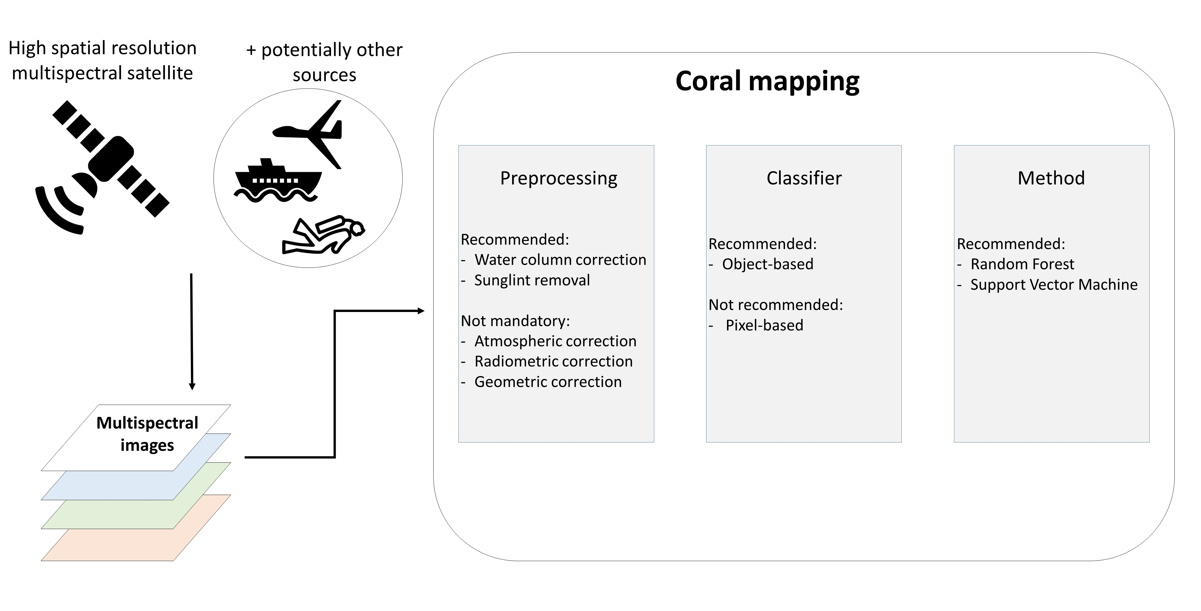
The worldwide decline of coral reefs has prompted an unprecedented research effort, reflected by the exponential growth of scientific articles dedicated to coral reefs (see Figure 1). A key prospect faced by the scientific community is the development of open and robust monitoring tools to survey the reef distribution on a global scale for the next decades. Mapping benthic reef habitats is crucially important for tracking their time and space evolution, with direct outcomes for reef geometry and health surveys [18], for developing numerical models of circulation and wave agitation in reef-lagoon systems [19,20] and for socio-economic and environmental management policies [21].
A powerful tool to survey coral reefs is coral mapping or coral classification. This involves using raw input data of a coral site, such as videos or images, extracting the characteristics of the ground and classifying the elements as coral, sand, seagrass, etc. To perform this mapping, there are two possibilities: manually extracting the characteristics, which is a highly accurate method but tedious and time consuming, or training machine-learning algorithms to easily do it in a short time but with a higher chance of misclassification. In this article, the terms “coral mapping” and “coral classification” will both refer to the same meaning being the “automatic machine-learning mapping” if not otherwise stated.
Coral mapping can be accurately achieved from underwater images, as done in most papers published in 2020 [22,23,24,25,26,27,28,29,30,31,32]. However, a major drawback of underwater images is that they are difficult to acquire at a satisfying time resolution for most remote places, thus making it unfeasible to have a worldwide global map with this kind of data. One solution is to use data from satellite imagery.
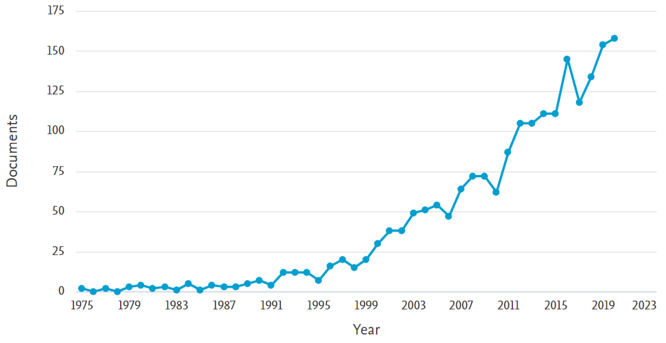
Aiming to help the ongoing and future efforts for coral mapping at the planetary scale, this paper will mainly focus on multispectral satellite images for coral classification and will mostly omit other sources of data. The main goal of this paper is to highlight the current most efficient methods and satellites to map coral reef. As depicted in Figure 1, there are twice as many papers published in the past two years than there were ten years ago. Furthermore, as described later, the resolution of satellites is quickly improving, and with it the accuracy of coral maps. This is also true for machine-learning methods and image processing. Finally, substantive reviews of work related to coral mapping are only available to 2017 [33,34]. For these reasons, we decided to narrow our analysis to papers published since 2018. Between 2018 and 2020, 446 documents tagging “coral mapping” or “coral remote sensing” have been published (Figure 1). However, most of these papers do not fit within the scope of our study: They are for instance treating tidal flats, biodiversity problems, chemical composition of the water, bathymetry retrieval, and so on. Thus, out of these 446, only 75 deal with coral classification or coral mapping problems. The data sources used in these papers are summarized in Figure 2. Within these 75 studies, a subset of 37 papers that deal with satellite data (25 with satellite data only) will be specifically included in the present study.
Used in almost 50% of the papers, satellite imagery is recommended by the Coral Reef Expert Group for habitat mapping and change detection on a broad scale [35]. It allows benthic habitat to be mapped more precisely than via local environmental knowledge [36] on a global scale, at frequent intervals and with an affordable price.
This review is divided into four parts. First, the different multispectral satellites are presented, and their performance compared. Following this is a review of the preprocessing steps that are often needed for analysis. The third part provides an overview of the most common automatic methods for mapping and classification based on satellite data. Finally, the paper will introduce some other technologies improving coral mapping.
2. Satellite Imagery
2.1. Spatial and Spectral Resolutions
When trying to classify benthic habitat, two conflicting parameters are generally put in balance for choosing the satellite image source: The spatial resolution (the surface represented by a pixel) and the spectral resolution. The latter generally refers to the number of available spectral bands, i.e., the precision of the wavelength detection by the sensor. The former parameter has a straightforward effect: a higher spatial resolution will allow a finer habitat mapping but will require a higher computational effort. The primary effect of the spectral resolution is that model accuracy generally increases with the number of visible bands [37,38,39] and the inclusion of infrared bands [40]. Although no clear definition exists, a distinction is generally made in terms of spectral resolution between multispectral and hyperspectral satellites. The former sensors produce images on a small number of bands, typically less than 20 or 30 channels, while hyperspectral sensors provide imagery data on a much larger number of narrow bands, up to several hundred—for instance NASA’s Hyperion imager with 220 channels. Most of the time, multispectral and hyperspectral sensors have an additional panchromatic band (capturing the wavelengths visible to the human eye) with a slightly higher spatial resolution than the other bands.
A major drawback of hyperspectral satellites is that the best achievable resolution is generally several tens of meters and can be up to 1 km for some of them [41], while most multispectral sensors have a resolution better than 4 m. A high spectral resolution coupled with a low-spatial-resolution result in a problem known as “spectral unmixing”, which is the process of decomposing a given mixed pixel into its component elements and their respective proportions. Some existing algorithms can tackle this issue with a high level of accuracy [42,43,44]. When unmixing pixels, algorithms may face errors due to the heterogeneity of seabed reflectance, disturbing the radiance with the light scattered on the neighboring elements [45]. This process, called the adjacency effect, has negative effects on the accuracy of remote sensing [46] and can modify the radiance by up to 26% depending on turbidity and water depth [47].
In this review, we purposefully omitted the hyperspectral sensors to focus on multispectral satellite sensors, since only the latter have a spatial resolution fine enough to map coral colonies. Moreover, in our case where we are studying how to create high-resolution maps of coral presence, multispectral satellites are more efficient, i.e., they provide more accurate results [35]. In the following parts, unless otherwise stated, the spatial resolution will be referred to as “resolution”.
2.2. Satellite Data
We found 14 different satellites appearing in benthic habitat mapping studies, and gathered in Table 1 their main characteristics, in particular their spectral bands, spatial resolution, revisit time and pricing. The Landsat satellites prior to Landsat 6 do not appear in the table because they are almost universally not used in recent studies, the Landsat 5 being deactivated in 2013.
The most commonly used multispectral satellite images are from NASA’s Landsat program [48]. The program relies on several satellites, of which Landsat 8 OLI, Landsat 7 ETM+, Landsat 6 ETM and Landsat TM have been used for benthic habitat mapping: [49,50,51,52,53] (OLI), [54,55,56] (OLI, ETM+, TM), [57,58,59,60] (ETM+). The standard revisit time for Landsat satellites is 16 days. However, Landsat-7 and Landsat-8 are offset so that their combined revisit time is 8 days. The density and accuracy of the Landsat images thus make them viable to use for ecological analyzes [61].
Sentinel-2 [62], a European Space Agency’s satellite, can be compared to Landsat satellites in terms of spatial and spectral resolution. Sentinel-2 was initially designed for land monitoring [63] but has been used for monitoring oceans (and more specifically coral reefs bleaching) and mapping benthic habitat [64,65,66,67,68,69,70]. Specific spectral bands of Sentinel-2, such as SWIR-cirrus and water vapor bands, are especially useful for cloud detection and removal algorithms [71,72,73,74,75]. One major advantage of Landsat and Sentinel-2 satellites is that their data are open access. However, these satellites are defined as “low-resolution”, with a resolution of tens of meters which may be a significant weakness when trying to map and to classify the fine and complex distribution of coral reef colonies.
With a typical spatial resolution of several meters, medium-resolution satellites are more accurate than the aforementioned satellites. Well-known medium-resolution satellites are SPOT-6 [76,77] and RapidEye [78,79,80], with respectively 4 and 5 bands. A major strength of RapidEye is that the image data are produced by a constellation of five identical satellites, thus providing images at a high frequency (global revisit time of one day). Note however that up to now, RapidEye has not been found in recent literature for coral mapping. The principle of using multiple similar satellites is also found with the PlanetScope constellation, composed of 130 Planet Dove satellites. Their total revisit time is less than one day, and they can be found in several recent coral mapping studies [81,82,83,84,85].
Finally, high-resolution sensors are defined as those with a few meters resolution, such as 3 m or less. IKONOS-2 belongs to this category and can be found in several studies of benthic habitat mapping [86,87,88,89], but mostly before 2015, the year it has ceased operating. GaoFen-2 satellite, launched in 2014, has the same spatial and spectral resolution as IKONOS-2, but is not as widely used [90], perhaps because of its age: It was launched in 2014, when some sensors already had a better resolution. GaoFen have different satellites (from GaoFen-1 to GaoFen-14) that have the same or a lower resolution than GaoFen-2.
With a similar sensor and a slightly better resolution than IKONOS-2, the Quickbird-2 satellite provides images for several studies of reef mapping [58,91,92,93,94,95,96]. Please note that the Quickbird-2 program was stopped in 2015. Similar features are proposed by the Pleiades-1 satellites, from the Optical and Radar Federated Earth Observation program, also present in the literature [97,98]. An even higher accuracy can be found with GeoEye-1 satellite, providing images at a resolution of less than 1m, making it particularly useful to study coral reefs [99].
The most common and most precise satellite images come from WorldView satellites. For instance, WorldView-2 (WV-2), launched in 2009, has been widely used for benthic habitat mapping and coastline extraction [40,76,90,100,101,102,103,104,105,106,107]. Despite the high-resolution images provided by WV-2, the highest quality images available at the current time come from WorldView-3 (WV-3), launched in 2014 [39,108,109,110]. WV-3 has a total of 16 spectral bands and is thus able to compete with hyperspectral sensors with more than a hundred bands (such as Hyperion). Moreover, its spatial resolution is the highest available among current satellites, and is even similar to local measurement techniques such as Unmanned Airborne Vehicles (UAV) [111]. Among all the spectral bands offered by the WV-3 sensors, the coastal blue band (400–450 nm) is especially useful for bathymetry, as this wavelength penetrates water more easily and may help to discriminate seagrass patterns [112]. Although the raw SWIR resolution is lower than the one achieved in visible and near-infrared bands, it can be further processed to generate high-resolution SWIR images [113]. In addition, the WV-3 panchromatic resolution is 0.3 m, which almost reaches the typical size of coral reef elements (0.25 m), thus making it also useful for reef monitoring [114].
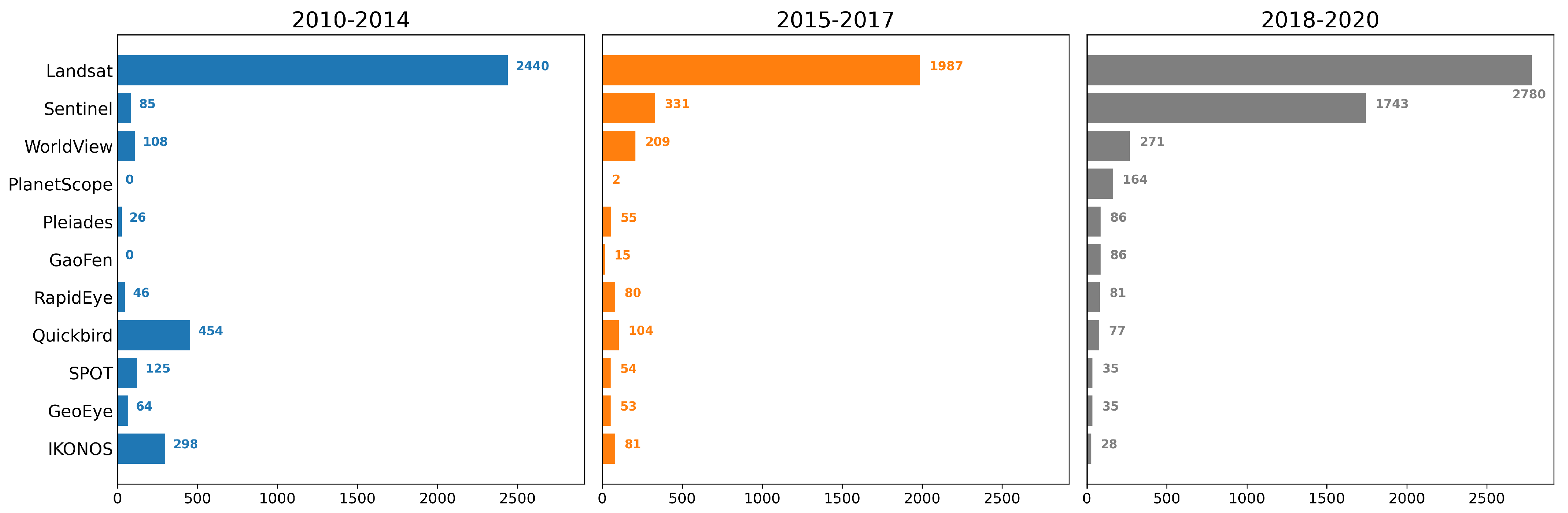
To further evaluate the importance of each satellite in the global literature (not only on coral studies) and to detect trends in their use, we searched in Scopus and analyzed the number of articles in which they appear between 2010 and 2020. Several trends can be seen. First, among low-resolution satellites, it appears that while the usage of Landsat remains stable over the year, the usage of Sentinel has exploded (by a multiplication factor of 20 between the period 2014–2014 and 2018–2020). Regarding high-resolution satellites, we detect trends in their usage: in the period 2010–2014, Quickbird and IKONOS satellites were predominant, but their usage decreased by more than 85% during the years 2018–2020. On the other hand, the number of papers published using WorldView and PlanetScope has been increasing: respectively from 108 and 0 in 2010–2014, to 271 and 164 in 2018–2020. The complete numbers for each satellite can be found in Figure A1.
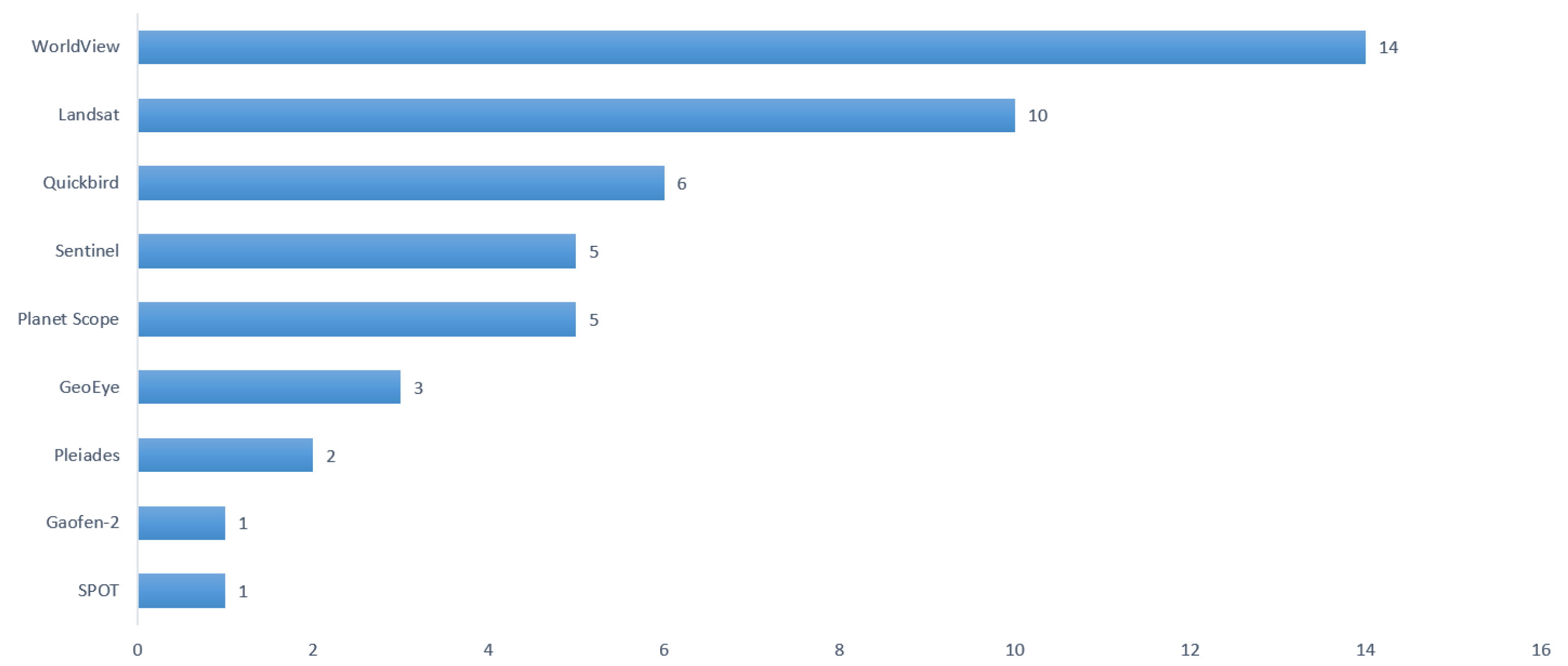
Figure 3 depicts which satellites were employed in the 37 studies using satellites (“satellite only” and “satellite + other” in Figure 2). Please note that some studies use data from more than one satellite. From this analysis, WorldView satellites appear to be the most commonly used ones for coral mapping, confirming that high-resolution multispectral satellites are more suitable than low-resolution ones for coral mapping.
3. Image Correction and Preprocessing
Even though satellite imagery is a unique tool for benthic habitat mapping, providing remote images at a relatively low cost over large time and space scales, it suffers from a variety of limitations. Some of these are not exclusively related to satellites but are shared with other remote sensing methods such as UAV. Most of the time, existing image correction methods can overcome these problems. In the same way, preprocessing methods often result in improved accuracy of classification. However, the efficiency of these algorithms is still not perfect and can sometimes induce noise when trying to create coral reef maps. This part will describe the most common processing that can be performed, as well as their limitations.
3.1. Clouds and Cloud Shadows
One major problem of remote sensing with satellite imagery is missing data, mainly caused by the presence of clouds and cloud shadows, and their effect on the atmosphere radiance measured on the pixels near clouds (adjacency effect) [115]. For instance, Landsat-7 images have on average a cloud coverage of 35% [116]. This problem is globally present, not only for the ocean-linked subjects but for every study using satellite images, such as land monitoring [117,118] and forest monitoring [119,120]. Thus, several algorithms have been developed in the literature to face this issue [121,122,123,124,125,126,127,128]. One widely used algorithm for cloud and cloud shadow detection is Function of mask, known as Fmask, for images from Landsat and Sentinel-2 satellites [129,130,131]. Given a multiband satellite image, this algorithm provides a mask giving a probability for each pixel to be cloud, and performs a segmentation of the image to segregate cloud and cloud shadow from other elements. However, the cloudy parts are just masked, but not replaced.
A common approach to remove cloud and clouds shadows is to create a composite image from multi-temporal images. This involves taking several images at different time periods but close enough to assume that no change has occurred in between, for instance over a few weeks [132]. These images are then combined to take the best cloud-free parts of each image to form one final composite image without clouds nor cloud shadows. This process is widely used [133,134,135,136] when a sufficient number of images is available.
3.2. Water Penetration and Benthic Heterogeneity
The issue of light penetration in water occurs not only with satellite imagery, but with all kinds of remote sensing imagery, including those provided by UAV or boats. The sunlight penetration is strongly limited by the light attenuation in water due to absorption, scattering and conversion to other forms of energy. Most sunlight is therefore unable to penetrate below the 20 m surface layer. Hence, the accuracy of a benthic mapping will decrease when the water depth increases [137]. The light attenuation is wavelength dependent, the stronger attenuation being observed either at short (ultraviolet) or long (infrared) wavelengths while weaker attenuation in the blue-green band allows deeper penetration. Specific spectral bands such as the green one may be viable for benthic habitat mapping and coral changes, such as bleaching [67]. As the penetration through water depends on the wavelength, image preprocessing may be needed to correct this effect. Water column correction methods enable retrieval of the real bottom reflectance from the reflectance captured by the sensor, using either band combination or algebraic computing depending on the method used. Using a water column correction method can improve the mapping accuracy by more than 20% [138,139]. Several models of water column correction exist, each of them with different performances [140], the best known one being Lyzenga’s [141]. The best model strongly depends on the input data and the desired result; see Zoffoli et al. 2014 [140] for a detailed overview of the water column correction methods.
When it is known that the water depth of the study field is homogeneous, it is possible to classify the benthic habitat without applying any correction [142]. However, even in a shallow environment that would be weakly impacted by the light penetration issue (i.e., typically less than 2 m deep), a phenomenon called spectral confusion can occur if the depth is not homogeneous [143]. At different depths, the response of two different-color elements can be similar on a wide part of the light spectrum. Hence, with an unknown depth variation, the spectral responses of elements such as dead corals, seagrasses, bleached corals and live corals can be mixed up and their separability significantly affected, making it harder to map correctly [144]. Nevertheless, this depth heterogeneity problem can be overcome: when mixing satellite images with in situ measurements (such as single-beam echo sounder), it is possible to have an accurate benthic mapping of reefs with complex structures in shallow waters [108]. However, the advantage of not needing ground-truth data (information collected on the ground) when working with satellite imagery is lost with this solution.
3.3. Light Scattering
When remotely observing a surface such as water, especially with satellite imagery, its reflectance may be influenced by the atmosphere. Two phenomena modify the reflectance measured by the sensor. First, the Rayleigh’s scattering causes smaller wavelengths (e.g., blue 400 nm) to be more scattered than larger ones (e.g., red 800 nm). Secondly, small particles present in the air cause so-called aerosol scattering, also altering the radiance perceived by the satellites [145,146]. Hence, the reflectance perceived by the satellite’s sensors is composed of the true reflectance to which are added both Rayleigh- and aerosol-related scattered components [147,148].
It is possible to apply algorithms to correct the effects due to Earth’s atmosphere [149,150,151], making some assumptions such as the horizontal homogeneity of the atmosphere, or the flatness of the ocean. However, these atmospheric corrections do not always result in a significant increase in the classification accuracy when using multispectral images [152], and they are not as frequent as water column corrections, which is why we consider them as optional.
3.4. Masking
Masking consists of removing geographic areas that are not useful or usable: clouds, cloud shadows, land, boats, wave breaks, and so on. Masking can improve the performance of some algorithms such as crop classification [153] or Sea Surface Temperature (SST) retrievals [154].
Even though highly accurate algorithms exist to detect most clouds, as discussed previously, some papers employ manual masking for higher accuracy [155]. It is also possible to mask deep water, in which coral reef mapping is difficult to achieve. Deep water to be masked can be defined by a criterion such as a reflectance threshold over the blue band (450–510 nm) [156].
3.5. Sunglint Removal
When working with water surfaces, such as an ocean or lagoon, sunglint poses a high risk of altering the quality of the image, not only for satellite imagery but for every remote sensing system. Sunglint happens when the sunlight is reflected on the water surface with an angle similar to the one the image is being taken with, often because of waves. Thus, higher solar angles induce more sunglint; on the other hand, they are also correlated with a better quality for bathymetry mapping based on physical analysis methods [155]. Although this reflectance can be easily avoided when taking field images from an airborne vehicle (by controlling the time of the day and the direction), it is harder to avoid with satellite imagery. It thus must be removed from the image for better accuracy of benthic habitat mapping. This can be achieved, for instance, by a simple linear regression [157]. Some other models can also efficiently tackle this issue [158,159,160,161]. According to Muslim et al. 2019 [162], the most efficient sunglint removal procedure when mapping coral reef from UAV is the one described in Lyzenga et al. 2006 [163]. As the procedures compared in the paper depend on multispectral UAV data, we can imagine that the result may be true for satellite data as well.
3.6. Geometric Correction
Geometric correction consists of georeferencing the satellite image by matching it to the coordinates of the elements on the ground. It allows, for instance, removal of spatial distortion from an image or drawing a parallel between two different sources of data, such as several satellite images, satellite images with other images (e.g., aerial), or images mixed with bathymetry inputs (sonar, LiDAR). This step is especially important in the case of satellite imagery, which is subject to a large number of variations such as angle, radiometry, resolution or acquisition mode [164].
Geometric corrections are needed to be able to use ground-truth control points. These data can take several forms, for instance divers’ underwater videos or acoustic measurements from a boat. Even though control points are not used in every study, they are frequent because they enable a high-quality error assessment and/or a more accurate training set. However, control points are not that easy to acquire because they require a field survey, which is not always possible and may be expensive for some remote sites. Thus, control points are not always used.
3.7. Radiometric Correction
When working with multi-temporal images of the same place, the series of images is likely to be heterogeneous because of some noise for instance induced by sensors, illumination, solar angle or atmospheric effects. Radiometric correction enables normalization of several images to make them consistent and comparable. Radiometric corrections significantly improve accuracy in change detection and classification algorithms [165,166,167,168]. Identically to geometric corrections that are only required when working with ground-truth control points, radiometric corrections are only needed when working with several images of the same place. Radiometric corrections are also useful to provide factors needed in the equations of some atmospheric correction algorithms [169].
3.8. Contextual Editing
Contextual editing is a postprocessing of the image, subsequent to the classification step that takes into account the surrounding pattern of an element [170,171]. Indeed, some classes cannot be surrounded by another given class, and if it is found to be the case then the classifier has probably made a mistake. For instance, an element classified as “land” that is surrounded by water elements is more likely to be a class such as “algae”.
The use of contextual editing can greatly enhance the performance of a classifier, be it for land area [172] or for coral reefs [138,173]. However, surprisingly, it appears that this method has not been widely employed in the published literature, especially with benthic habitat related topics. To the best of our knowledge, even though we found some papers using contextual editing for bathymetry studies, it has not been applied to coral reef mapping in the past 10 years.
4. From Images to Coral Maps
Satellite imagery represents a powerful tool to assess coral maps, should we be able to tackle the problems that come with it. Manual mapping of coral reefs from a given image is a long and arduous work and synthetic expert mapping over large spatial area and/or long time periods is definitely out of reach, especially when the area to be mapped has a size of several km. Coral habitats are at the moment unequally studied, with some sites that are almost not analyzed at all by scientists: for instance, studies on cold-water corals mostly focus on North-East Atlantic [174]. The development of automated processing algorithms is a necessary step to target a worldwide and long-term monitoring of corals from satellite images. The mapping of coral reefs from remote sensing usually follows the flow chart given in Andréfouët 2008 [175] consisting of several steps of image corrections, as seen previously, followed by image classification. For instance, with one exception, all the studies published since 2018 that deal with mapping coral reefs from satellite images perform at least three out of the four preprocessing steps given in [175]. The following subsections provide a comparison of the accuracies given by different statistical and machine-learning methods.
4.1. Pixel-Based and Object-Based
Before comparing the machine-learning methods, a difference must be drawn between two main ways to classify a map: pixel-based and object-based. The first consists of taking each pixel separately and assigning it a class (e.g., coral, sand, seagrass, etc.) without taking into account neighboring pixels. The second consists of taking an object (i.e., a whole group of pixels) and giving it a class depending on the interaction of the elements inside of it.
The object-based image analysis method performs well for high-resolution images, due to a high heterogeneity of pixels which is not suited for pixel-based approaches [176]. This implies that object-based methods should be used in the study of reef changes working with high-resolution multispectral satellite images instead of low-resolution hyperspectral satellite images. Indeed, the object-based method has an accuracy 15% to 20% higher than the pixel-based one in the case of reef change detection [156,177,178] and benthic habitats mapping [77,179].
The relative superiority of the object-based approach has also been shown when applied to land classification [180,181], such as bamboo mapping [182] or tree classification [183,184]. Nonetheless, even if the object-based methods are generally more accurate, they remain harder to set up because they need to perform a segmentation step (to create the objects) before the classification.
4.2. Maximum Likelihood
Maximum likelihood (MLH) classifiers are particularly efficient when the seabed does not have a too complex architecture [185]. With good image condition, i.e., clear shallow water (<7 m) and almost no cloud cover, a MLH classifier can discriminate Acropora spp. corals from other classes (sand, seagrass, mixed coral species) with an accuracy of 90% [186]. Moreover, a MLH classifier works well under two conditions: when the spectral responses of the habitats are different enough to be discriminated, and when the area analyzed is in shallow waters ( m) [87]. It is however very likely that these results can be applied to other machine-learning methods.
Nevertheless, when compared to other classification methods such as Support Vector Machine (SVM) or Neural Networks (NN), MLH classifiers appear to be less efficient, be it for land classification [152,187,188,189,190] or for coastline extraction [103,191]. A comparison of some algorithms applied to crop classification also confirms that SVM and NN perform better, with an accuracy of more than 92% [192].
4.3. Support Vector Machine
Across several studies, SVM appears to be the method with the best accuracy [187,188,193], especially with edge pixels, i.e., pixels which border two different classes [191]. In the studies published between 2018 and 2020, SVM classifiers had on average an accuracy of 70% for coral mapping, but can achieve up to 93% classification accuracy among 9 different classes of benthic habitat [194] when coupling high-resolution satellite images from WV-3 with drone images [194].
4.4. Random Forest
Random Forest (RF) methods also are very efficient in remote sensing classification problems [195]. They perform well to classify and map seagrass meadows [196] or land-use [197], the most often forests [198,199,200], although performance for land ecosystems may not be directly compared to that obtained for marine habitat mapping. For shallow water benthic mapping, a RF classifier can still outperform a SVM classifier in benthic habitat mapping [185], or at least have an identical overall accuracy but with a better spatial distribution. Globally, RF classifiers can map benthic habitat with an overall accuracy ranging from 60% to 85% [85,201,202,203,204,205], depending on the study site, the satellite imagery involved, and the preprocessing steps applied to the images.
4.5. Neural Networks
NN are commonly used to classify coral species with underwater images, but to date have rarely been used to map coral reefs from satellite images alone [90,206,207]. However, NN often appear in papers where satellite images are mixed with other sources such as aerial photographs, bathymetry data, or underwater images [208,209]. NN can be useful to perform a segmentation to extract features before performing the classification with a more common machine-learning method such as SVM [90] or K-nearest neighbors, with more than 80% mapping accuracy [207].
4.6. Unsupervised Methods
Unsupervised machine-learning methods are less frequent but still appear in some studies. The most present methods are based on K-means and ISODATA [65,68,77] with an accuracy ranging from 50% to 80%, reaching 92% when discriminating between 3 benthic classes [81]. The latter is an improvement of the former, where the user does not have to specify the number of clusters as an input. In the first place, the algorithm clusters the data, and then assign each cluster a class.
4.7. Synthesis
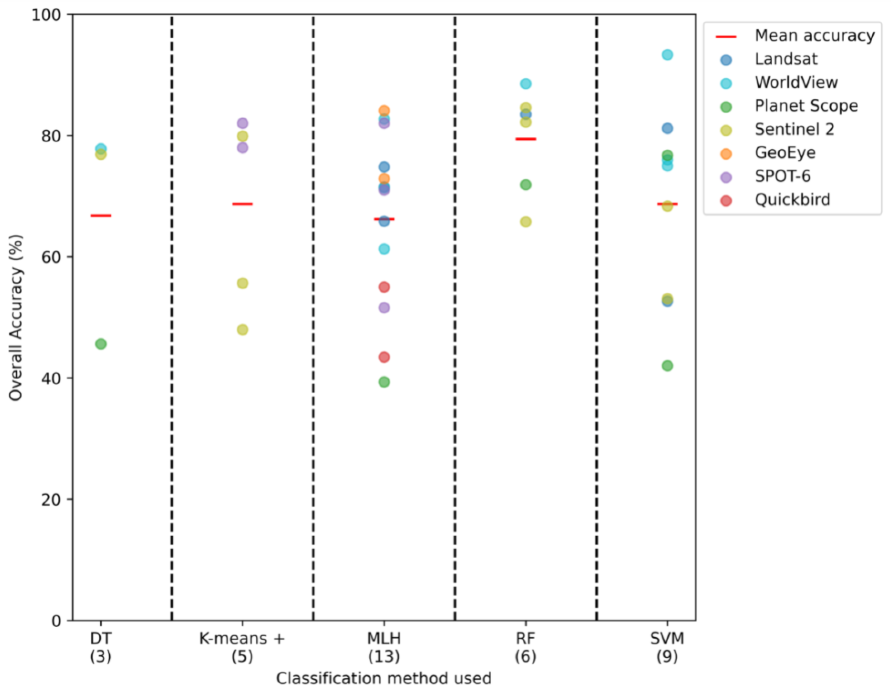
Given that the results on which is the best classifier can vary from a paper to another, we decided to gather in Figure 4 the coral mapping studies since 2018 using satellite imagery only. Please note that we excluded the methods that appeared in less than 3 papers, leading to an analysis of a subset of 20 study of the 25 papers depicted in Figure 2. We regrouped the methods K-means and ISODATA under the same label “K-means +” because these two methods are based on the same clustering process. Despite our comprehensive search of the literature, we acknowledge the possibility that some studies may have been overlooked. All the papers used here can be found in Table A1.
From the previous section and Figure A1, we recommend that the most accurate methods are RF and SVM. However, this recommendation has to be carefully evaluated because all the studies compared in this paper are based on different methods (how the performance of the model is evaluated and which preprocessing are performed on the images) and data sets (location of the study site and satellite images used), which may have a strong influence on the obtained results.
5. Improving Accuracy of Coral Maps
Although we have focused so far on satellite images-derived maps, there are many other ways to locate coral reefs without directly mapping them. This section will describe how to study reefs without necessarily mapping them, and the technologies that allow improvements in the precision of reef mapping.
5.1. Indirect Sensing
It is possible to acquire information on reefs and their localization without directly mapping them. Indirect sensing refers to these methods, studying reefs by analyzing their surrounding factors.
For instance, measuring Sea Surface Temperatures (SST) have helped to draw conclusions that corals have already started adapting to the rise of ocean temperature [17]. Similarly, as anomalies in SST are an important factor in coral outplant survival [210], an algorithm forecasting SST can predict which heat stress may cause a coral bleaching event [211]. Furthermore, it is possible to use deep neural networks to predict SST even more accurately [212]. However, even though the measured SST and the real temperature experienced by reefs can be similar [213], it is not always the case depending on the sensors used and other measurements such as wind, waves and seasons [214]. To try to overcome this issue and obtain finer predictions of the severity of bleaching events, it is possible to combine water temperature with other factors such as the light stress factor [215], known to be a cause of bleaching [216].
Backscatter and absorption measurements, as well as chlorophyll-a levels, can also be analyzed to detect reef changes [217,218]. The chlorophyll-a levels and total suspended matter can be highly accurately retrieved with some algorithms based on satellite images [219,220,221,222]. Similarly, computation on bottom reflectance can detect coral bleaching [223].
We could imagine that these indirect measurements, performed with satellite imagery and providing useful data about coral health, could be incorporated as an additional input to some classifiers to improve their accuracy. This is something we have not been able to find in current literature and that we suggest trying.
5.2. Additional Inputs to Coral Mapping
First, to enhance the classification accuracy, it appears evident that a higher satellite image resolution implies a higher accuracy for a same algorithm [224]. Notwithstanding this, we will describe here the different means to enhance the mapping with a given satellite resolution.
To be able to effectively detect environmental changes, several factors are important [225], among which the quality of the satellite images [226] and the quantity of data over time [227]. Indeed, it is essential to have a temporal resolution of a few days or even less, to be able to select the best images, without cloud nor sunglint [228]. A solution can thus be to couple images from a high-resolution satellite with a high-frequency satellite, for instance WV-3 and RapidEye [194].
To be able to discriminate some coral reefs with a special topography, satellite imagery may not be enough. Adding bathymetry data, for instance acquired with LiDAR, can improve the accuracy of the results [88,156,229,230,231]. It is possible to estimate bathymetry and water depth, with one of a numbered methods that currently exist [232,233,234,235], and to include this as an additional input to a coral reef mapping algorithm [236]. This method is found in Collin et al. 2021 [39], where it improves the accuracy by up to 3%, allowing more than 98% overall accuracy with high-resolution WV-3 images.
5.3. Citizen Science
Crowd sourcing can help classify images or provide large sets of data [244,245,246,247,248,249,250], in remote sensing of coral reefs as well as in other fields. However, the citizen scientists can be wrong or provide different classification [251,252,253] and thus still some modifications are often needed to learn from citizens’ responses [254,255]. The Neural Multimodal Observation and Training Network (NeMO-Net), a NASA project, is a good example of how citizen science can be used to generate highly accurate 3D maps and provide a global reef assessment, based on an interactive classification game [207,256,257]. This type of data can especially be helpful to feed a neural network, knowing that ground-truth knowledge and expert classification are hard to acquire.
6. Conclusions and Recommendations
Through all the papers studying coral reefs between 2018 and 2020 and mapping them from satellite imagery, the best results are obtained with RF and SVM methods, even though the achieved overall accuracy almost never reaches 90%, and is often below 80%. The arrival of very high-resolution satellites dramatically increases this to more than 98% [39]. To map coral reefs with a higher accuracy, we recommend using satellite images with additional inputs when it is possible.
When performing coral mapping from satellite images, it is very common to apply a wide range of preprocessing. Out of the four preprocessing methods proposed in Andréfouët 2008 [175], we suggest applying a water column correction (see [140] for the best method), and a sunglint correction (we recommend [163]). Geometric correction is only needed when working with ground-truth points, and radiometric correction when working with multi-temporal images. Interestingly, some postprocessing methods such as contextual editing appear to be less well used and could improve accuracy [138,173].
Presently, several projects exist to study and map coral reefs at a worldwide scale, using an array of resources, from satellite imagery to bathymetry data or underwater photographs: The Millennium Coral Reef Mapping Project [258], the Allen Coral Atlas [241] or the Khaled bin Sultan Living Ocean Foundation [259]. These maps are proven useful to the scientific community for coral reef and biodiversity monitoring and modeling, as well as inventories or socio-economic studies [260].
However, when examining the maps created by all these projects, we can see that many sites are yet to be studied. Furthermore, some reef systems have been mapped at a given time but would need to be analyzed more frequently, to be able to detect changes and obtain a better understanding of the current situation. Hence, even if the work achieved to date by the scientific community is huge, a lot still needs to be done. Great promise lies in upcoming very high-resolution satellites coupled with the cutting-edge technology of machine-learning algorithms.
Author Contributions
Writing—original draft preparation, T.N.; writing–review and editing, B.L., K.M. and D.S. All authors have read and agreed to the published version of the manuscript.
Funding
This study was sponsored by the BIGSEES project (E2S/UPPA).
Institutional Review Board Statement
This research received no external funding.
Conflicts of Interest
The authors declare no conflict of interest.
Abbreviations
The following abbreviations are used in this manuscript:
| CAVIS | Cloud, Aerosol, water Vapor, Ice, Snow |
| DT | Decision Tree |
| MLH | Maximum Likelihood |
| NN | Neural Networks |
| RF | Random Forest |
| SST | Sea Surface Temperatures |
| SVM | Support Vector Machine |
| SWIR | Short-Wave Infrared |
| UAV | Unmanned Airborne Vehicles |
| VNIR | Visible and Near-Infrared |
| WV-2 | WorldView-2 |
| WV-3 | WorldView-3 |
Appendix A
Figure A1 depicts the number of articles in which each satellite appears in Scopus, for three different periods: 2010–2014, 2015–2017, 2018–2020.
Figure A1.
Number of articles in which each satellite appears in the Scopus database, depending on the years.
Figure A1.
Number of articles in which each satellite appears in the Scopus database, depending on the years.

Appendix B

Table A1.
Studies from 2018 to 2020 used to compare the accuracies of different methods.
| Reference | Satellite Used | Method Used | Number of Classes |
|---|---|---|---|
| Ahmed et al. 2020 [203] | Landsat | RF, SVM | 4 |
| Anggoro et al. 2018 [179] | WV-2 | SVM | 9 |
| Aulia et al. 2020 [49] | Landsat | MLH | 6 |
| Fahlevi et al. 2018 [59] | Landsat | MLH | 4 |
| Gapper et al. 2019 [52] | Landsat | SVM | 2 |
| Hossain et al. 2019 [91] | Quickbird | MLH | 4 |
| Hossain et al. 2020 [92] | Quickbird | MLH | 4 |
| Immordino et al. 2019 [65] | Sentinel-2 | ISODATA | 10 and 12 |
| Lazuardi et al. 2021 [205] | Sentinel-2 | RF, SVM | 4 |
| McIntyre et al. 2018 [224] | GeoEye-1 and WV-2 | MLH | 3 |
| Naidu et al. 2018 [104] | WV-2 | MLH | 7 |
| Poursanidis et al. 2020 [204] | Sentinel-2 | DT, RF, SVM | 4 |
| Rudiastuti et al. 2021 [68] | Sentinel-2 | ISODATA, K-Means | 4 |
| Shapiro et al. 2020 [69] | Sentinel-2 | RF | 4 |
| Siregar et al. 2020 [76] | WV-2 and SPOT-6 | MLH | 8 |
| Sutrisno et al. 2021 [77] | SPOT-6 | K-Means, ISODATA, MLH | 4 |
| Wicaksono & Lazuardi 2018 [84] | Planet Scope | DT, MLH, SVM | 5 |
| Wicaksono et al. 2019 [185] | WV-2 | DT, RF, SVM | 4 and 14 |
| Xu et al. 2019 [107] | WV-2 | SVM, MLH | 5 |
| Zhafarina & Wicaksono 2019 [85] | Planet Scope | RF, SVM | 3 |
References
- Gibson, R.; Atkinson, R.; Gordon, J.; Smith, I.; Hughes, D. Coral-associated invertebrates: Diversity, ecological importance and vulnerability to disturbance. In Oceanography and Marine Biology; Taylor & Francis: Oxford, UK, 2011; Volume 49, pp. 43–104. [Google Scholar]
- Wolfe, K.; Anthony, K.; Babcock, R.C.; Bay, L.; Bourne, D.G.; Burrows, D.; Byrne, M.; Deaker, D.J.; Diaz-Pulido, G.; Frade, P.R.; et al. Priority species to support the functional integrity of coral reefs. In Oceanography and Marine Biology; Taylor & Francis: Oxford, UK, 2020. [Google Scholar]
- Spalding, M.; Grenfell, A. New estimates of global and regional coral reef areas. Coral Reefs 1997, 16, 225–230. [Google Scholar] [CrossRef]
- Costello, M.J.; Cheung, A.; De Hauwere, N. Surface area and the seabed area, volume, depth, slope, and topographic variation for the world’s seas, oceans, and countries. Environ. Sci. Technol. 2010, 44, 8821–8828. [Google Scholar] [CrossRef]
- Reaka-Kudla, M.L. The global biodiversity of coral reefs: A comparison with rain forests. Biodivers. II Underst. Prot. Our Biol. Resour. 1997, 2, 551. [Google Scholar]
- Roberts, C.M.; McClean, C.J.; Veron, J.E.; Hawkins, J.P.; Allen, G.R.; McAllister, D.E.; Mittermeier, C.G.; Schueler, F.W.; Spalding, M.; Wells, F.; et al. Marine biodiversity hotspots and conservation priorities for tropical reefs. Science 2002, 295, 1280–1284. [Google Scholar] [CrossRef] [PubMed] [Green Version]
- Martínez, M.L.; Intralawan, A.; Vázquez, G.; Pérez-Maqueo, O.; Sutton, P.; Landgrave, R. The coasts of our world: Ecological, economic and social importance. Ecol. Econ. 2007, 63, 254–272. [Google Scholar] [CrossRef]
- Riegl, B.; Johnston, M.; Purkis, S.; Howells, E.; Burt, J.; Steiner, S.C.; Sheppard, C.R.; Bauman, A. Population collapse dynamics in Acropora downingi, an Arabian/Persian Gulf ecosystem-engineering coral, linked to rising temperature. Glob. Chang. Biol. 2018, 24, 2447–2462. [Google Scholar] [CrossRef] [PubMed]
- Putra, R.; Suhana, M.; Kurniawn, D.; Abrar, M.; Siringoringo, R.; Sari, N.; Irawan, H.; Prayetno, E.; Apriadi, T.; Suryanti, A. Detection of reef scale thermal stress with Aqua and Terra MODIS satellite for coral bleaching phenomena. In AIP Conference Proceedings; AIP Publishing LLC: Melville, NY, USA, 2019; Volume 2094, p. 020024. [Google Scholar]
- Sully, S.; Burkepile, D.; Donovan, M.; Hodgson, G.; Van Woesik, R. A global analysis of coral bleaching over the past two decades. Nat. Commun. 2019, 10, 1264. [Google Scholar] [CrossRef] [Green Version]
- Glynn, P.; Peters, E.C.; Muscatine, L. Coral tissue microstructure and necrosis: Relation to catastrophic coral mortality in Panama. Dis. Aquat. Org. 1985, 1, 29–37. [Google Scholar] [CrossRef]
- Ortiz, J.C.; Wolff, N.H.; Anthony, K.R.; Devlin, M.; Lewis, S.; Mumby, P.J. Impaired recovery of the Great Barrier Reef under cumulative stress. Sci. Adv. 2018, 4, eaar6127. [Google Scholar] [CrossRef] [PubMed] [Green Version]
- Pratchett, M.S.; Munday, P.; Wilson, S.K.; Graham, N.; Cinner, J.E.; Bellwood, D.R.; Jones, G.P.; Polunin, N.; McClanahan, T. Effects of climate-induced coral bleaching on coral-reef fishes. Ecol. Econ. Conseq. Oceanogr. Mar. Biol. Annu. Rev. 2008, 46, 251–296. [Google Scholar]
- Hughes, T.P.; Kerry, J.T.; Baird, A.H.; Connolly, S.R.; Chase, T.J.; Dietzel, A.; Hill, T.; Hoey, A.S.; Hoogenboom, M.O.; Jacobson, M.; et al. Global warming impairs stock–Recruitment dynamics of corals. Nature 2019, 568, 387–390. [Google Scholar] [CrossRef] [PubMed]
- Schoepf, V.; Carrion, S.A.; Pfeifer, S.M.; Naugle, M.; Dugal, L.; Bruyn, J.; McCulloch, M.T. Stress-resistant corals may not acclimatize to ocean warming but maintain heat tolerance under cooler temperatures. Nat. Commun. 2019, 10, 4031. [Google Scholar] [CrossRef] [PubMed] [Green Version]
- Hughes, T.P.; Anderson, K.D.; Connolly, S.R.; Heron, S.F.; Kerry, J.T.; Lough, J.M.; Baird, A.H.; Baum, J.K.; Berumen, M.L.; Bridge, T.C.; et al. Spatial and temporal patterns of mass bleaching of corals in the Anthropocene. Science 2018, 359, 80–83. [Google Scholar] [CrossRef] [PubMed] [Green Version]
- Logan, C.A.; Dunne, J.P.; Eakin, C.M.; Donner, S.D. Incorporating adaptive responses into future projections of coral bleaching. Glob. Chang. Biol. 2014, 20, 125–139. [Google Scholar] [CrossRef]
- Graham, N.; Nash, K. The importance of structural complexity in coral reef ecosystems. Coral Reefs 2013, 32, 315–326. [Google Scholar] [CrossRef]
- Sous, D.; Tissier, M.; Rey, V.; Touboul, J.; Bouchette, F.; Devenon, J.L.; Chevalier, C.; Aucan, J. Wave transformation over a barrier reef. Cont. Shelf Res. 2019, 184, 66–80. [Google Scholar] [CrossRef] [Green Version]
- Sous, D.; Bouchette, F.; Doerflinger, E.; Meulé, S.; Certain, R.; Toulemonde, G.; Dubarbier, B.; Salvat, B. On the small-scale fractal geometrical structure of a living coral reef barrier. Earth Surf. Process. Landf. 2020, 45, 3042–3054. [Google Scholar] [CrossRef]
- Harris, P.T.; Baker, E.K. Why map benthic habitats. In Seafloor Geomorphology as Benthic Habitat; Elsevier: Amsterdam, The Netherlands, 2012; pp. 3–22. [Google Scholar]
- Gomes, D.; Saif, A.S.; Nandi, D. Robust Underwater Object Detection with Autonomous Underwater Vehicle: A Comprehensive Study. In Proceedings of the International Conference on Computing Advancements, Dhaka, Bangladesh, 10–12 January 2020; pp. 1–10. [Google Scholar]
- Long, S.; Sparrow-Scinocca, B.; Blicher, M.E.; Hammeken Arboe, N.; Fuhrmann, M.; Kemp, K.M.; Nygaard, R.; Zinglersen, K.; Yesson, C. Identification of a soft coral garden candidate vulnerable marine ecosystem (VME) using video imagery, Davis Strait, west Greenland. Front. Mar. Sci. 2020, 7, 460. [Google Scholar] [CrossRef]
- Mahmood, A.; Bennamoun, M.; An, S.; Sohel, F.; Boussaid, F. ResFeats: Residual network based features for underwater image classification. Image Vis. Comput. 2020, 93, 103811. [Google Scholar] [CrossRef]
- Marre, G.; Braga, C.D.A.; Ienco, D.; Luque, S.; Holon, F.; Deter, J. Deep convolutional neural networks to monitor coralligenous reefs: Operationalizing biodiversity and ecological assessment. Ecol. Inform. 2020, 59, 101110. [Google Scholar] [CrossRef]
- Mizuno, K.; Terayama, K.; Hagino, S.; Tabeta, S.; Sakamoto, S.; Ogawa, T.; Sugimoto, K.; Fukami, H. An efficient coral survey method based on a large-scale 3-D structure model obtained by Speedy Sea Scanner and U-Net segmentation. Sci. Rep. 2020, 10, 12416. [Google Scholar] [CrossRef]
- Modasshir, M.; Rekleitis, I. Enhancing Coral Reef Monitoring Utilizing a Deep Semi-Supervised Learning Approach. In Proceedings of the 2020 IEEE International Conference on Robotics and Automation (ICRA), Paris, France, 31 May–31 August 2020; IEEE: Piscataway, NJ, USA, 2020; pp. 1874–1880. [Google Scholar]
- Paul, M.A.; Rani, P.A.J.; Manopriya, J.L. Gradient Based Aura Feature Extraction for Coral Reef Classification. Wirel. Pers. Commun. 2020, 114, 149–166. [Google Scholar] [CrossRef]
- Raphael, A.; Dubinsky, Z.; Iluz, D.; Benichou, J.I.; Netanyahu, N.S. Deep neural network recognition of shallow water corals in the Gulf of Eilat (Aqaba). Sci. Rep. 2020, 10, 1–11. [Google Scholar] [CrossRef]
- Thum, G.W.; Tang, S.H.; Ahmad, S.A.; Alrifaey, M. Toward a Highly Accurate Classification of Underwater Cable Images via Deep Convolutional Neural Network. J. Mar. Sci. Eng. 2020, 8, 924. [Google Scholar] [CrossRef]
- Villanueva, M.B.; Ballera, M.A. Multinomial Classification of Coral Species using Enhanced Supervised Learning Algorithm. In Proceedings of the 2020 IEEE 10th International Conference on System Engineering and Technology (ICSET), Shah Alam, Malaysia, 9 November 2020; IEEE: Piscataway, NJ, USA, 2020; pp. 202–206. [Google Scholar]
- Yasir, M.; Rahman, A.U.; Gohar, M. Habitat mapping using deep neural networks. Multimed. Syst. 2021, 27, 679–690. [Google Scholar] [CrossRef]
- Hamylton, S.M.; Duce, S.; Vila-Concejo, A.; Roelfsema, C.M.; Phinn, S.R.; Carvalho, R.C.; Shaw, E.C.; Joyce, K.E. Estimating regional coral reef calcium carbonate production from remotely sensed seafloor maps. Remote Sens. Environ. 2017, 201, 88–98. [Google Scholar] [CrossRef]
- Purkis, S.J. Remote sensing tropical coral reefs: The view from above. Annu. Rev. Mar. Sci. 2018, 10, 149–168. [Google Scholar] [CrossRef] [PubMed]
- Gonzalez-Rivero, M.; Roelfsema, C.; Lopez-Marcano, S.; Castro-Sanguino, C.; Bridge, T.; Babcock, R. Supplementary Report to the Final Report of the Coral Reef Expert Group: S6. Novel Technologies in Coral Reef Monitoring; Great Barrier Reef Marine Park Authority: Townsville, QLD, Australia, 2020. [Google Scholar]
- Selgrath, J.C.; Roelfsema, C.; Gergel, S.E.; Vincent, A.C. Mapping for coral reef conservation: Comparing the value of participatory and remote sensing approaches. Ecosphere 2016, 7, e01325. [Google Scholar] [CrossRef] [Green Version]
- Botha, E.J.; Brando, V.E.; Anstee, J.M.; Dekker, A.G.; Sagar, S. Increased spectral resolution enhances coral detection under varying water conditions. Remote Sens. Environ. 2013, 131, 247–261. [Google Scholar] [CrossRef]
- Manessa, M.D.M.; Kanno, A.; Sekine, M.; Ampou, E.E.; Widagti, N.; As-syakur, A. Shallow-water benthic identification using multispectral satellite imagery: Investigation on the effects of improving noise correction method and spectral cover. Remote Sens. 2014, 6, 4454–4472. [Google Scholar] [CrossRef] [Green Version]
- Collin, A.; Andel, M.; Lecchini, D.; Claudet, J. Mapping Sub-Metre 3D Land-Sea Coral Reefscapes Using Superspectral WorldView-3 Satellite Stereoimagery. Oceans 2021, 2, 18. [Google Scholar] [CrossRef]
- Collin, A.; Archambault, P.; Planes, S. Bridging ridge-to-reef patches: Seamless classification of the coast using very high resolution satellite. Remote Sens. 2013, 5, 3583–3610. [Google Scholar] [CrossRef] [Green Version]
- Hedley, J.D.; Roelfsema, C.M.; Chollett, I.; Harborne, A.R.; Heron, S.F.; Weeks, S.; Skirving, W.J.; Strong, A.E.; Eakin, C.M.; Christensen, T.R.; et al. Remote sensing of coral reefs for monitoring and management: A review. Remote Sens. 2016, 8, 118. [Google Scholar] [CrossRef] [Green Version]
- Bioucas-Dias, J.M.; Plaza, A.; Dobigeon, N.; Parente, M.; Du, Q.; Gader, P.; Chanussot, J. Hyperspectral Unmixing Overview: Geometrical, Statistical, and Sparse Regression-Based Approaches. IEEE J. Sel. Top. Appl. Earth Obs. Remote Sens. 2012, 5, 354–379. [Google Scholar] [CrossRef] [Green Version]
- Wang, X.; Zhong, Y.; Zhang, L.; Xu, Y. Blind hyperspectral unmixing considering the adjacency effect. IEEE Trans. Geosci. Remote Sens. 2019, 57, 6633–6649. [Google Scholar] [CrossRef]
- Guillaume, M.; Minghelli, A.; Deville, Y.; Chami, M.; Juste, L.; Lenot, X.; Lafrance, B.; Jay, S.; Briottet, X.; Serfaty, V. Mapping Benthic Habitats by Extending Non-Negative Matrix Factorization to Address the Water Column and Seabed Adjacency Effects. Remote Sens. 2020, 12, 2072. [Google Scholar] [CrossRef]
- Guillaume, M.; Michels, Y.; Jay, S. Joint estimation of water column parameters and seabed reflectance combining maximum likelihood and unmixing algorithm. In Proceedings of the 2015 7th Workshop on Hyperspectral Image and Signal Processing: Evolution in Remote Sensing (WHISPERS), Tokyo, Japan, 2–5 June 2015; pp. 1–4. [Google Scholar]
- Bulgarelli, B.; Kiselev, V.; Zibordi, G. Adjacency effects in satellite radiometric products from coastal waters: A theoretical analysis for the northern Adriatic Sea. Appl. Opt. 2017, 56, 854–869. [Google Scholar] [CrossRef]
- Chami, M.; Lenot, X.; Guillaume, M.; Lafrance, B.; Briottet, X.; Minghelli, A.; Jay, S.; Deville, Y.; Serfaty, V. Analysis and quantification of seabed adjacency effects in the subsurface upward radiance in shallow waters. Opt. Express 2019, 27, A319–A338. [Google Scholar] [CrossRef] [PubMed]
- Rajeesh, R.; Dwarakish, G. Satellite oceanography—A review. Aquat. Procedia 2015, 4, 165–172. [Google Scholar] [CrossRef]
- Aulia, Z.S.; Ahmad, T.T.; Ayustina, R.R.; Hastono, F.T.; Hidayat, R.R.; Mustakin, H.; Fitrianto, A.; Rifanditya, F.B. Shallow Water Seabed Profile Changes in 2016–2018 Based on Landsat 8 Satellite Imagery (Case Study: Semak Daun Island, Karya Island and Gosong Balik Layar). Omni-Akuatika 2020, 16, 26–32. [Google Scholar] [CrossRef]
- Chegoonian, A.M.; Mokhtarzade, M.; Zoej, M.J.V.; Salehi, M. Soft supervised classification: An improved method for coral reef classification using medium resolution satellite images. In Proceedings of the 2016 IEEE International Geoscience and Remote Sensing Symposium (IGARSS), Beijing, China, 10–15 July 2016; pp. 2787–2790. [Google Scholar]
- Gapper, J.J.; El-Askary, H.; Linstead, E.; Piechota, T. Evaluation of spatial generalization characteristics of a robust classifier as applied to coral reef habitats in remote islands of the Pacific Ocean. Remote Sens. 2018, 10, 1774. [Google Scholar] [CrossRef] [Green Version]
- Gapper, J.J.; El-Askary, H.; Linstead, E.; Piechota, T. Coral Reef change Detection in Remote Pacific islands using support vector machine classifiers. Remote Sens. 2019, 11, 1525. [Google Scholar] [CrossRef] [Green Version]
- Iqbal, A.; Qazi, W.A.; Shahzad, N.; Nazeer, M. Identification and mapping of coral reefs using Landsat 8 OLI in Astola Island, Pakistan coastal ocean. In Proceedings of the 2018 14th International Conference on Emerging Technologies (ICET), Islamabad, Pakistan, 21–22 November 2018; pp. 1–6. [Google Scholar]
- El-Askary, H.; Abd El-Mawla, S.; Li, J.; El-Hattab, M.; El-Raey, M. Change detection of coral reef habitat using Landsat-5 TM, Landsat 7 ETM+ and Landsat 8 OLI data in the Red Sea (Hurghada, Egypt). Int. J. Remote Sens. 2014, 35, 2327–2346. [Google Scholar] [CrossRef]
- Gazi, M.Y.; Mowsumi, T.J.; Ahmed, M.K. Detection of Coral Reefs Degradation using Geospatial Techniques around Saint Martin’s Island, Bay of Bengal. Ocean. Sci. J. 2020, 55, 419–431. [Google Scholar] [CrossRef]
- Nurdin, N.; Komatsu, T.; AS, M.A.; Djalil, A.R.; Amri, K. Multisensor and multitemporal data from Landsat images to detect damage to coral reefs, small islands in the Spermonde archipelago, Indonesia. Ocean. Sci. J. 2015, 50, 317–325. [Google Scholar] [CrossRef]
- Andréfouët, S.; Muller-Karger, F.E.; Hochberg, E.J.; Hu, C.; Carder, K.L. Change detection in shallow coral reef environments using Landsat 7 ETM+ data. Remote Sens. Environ. 2001, 78, 150–162. [Google Scholar] [CrossRef]
- Andréfouët, S.; Guillaume, M.M.; Delval, A.; Rasoamanendrika, F.; Blanchot, J.; Bruggemann, J.H. Fifty years of changes in reef flat habitats of the Grand Récif of Toliara (SW Madagascar) and the impact of gleaning. Coral Reefs 2013, 32, 757–768. [Google Scholar] [CrossRef]
- Fahlevi, A.R.; Osawa, T.; Arthana, I.W. Coral Reef and Shallow Water Benthic Identification Using Landsat 7 ETM+ Satellite Data in Nusa Penida District. Int. J. Environ. Geosci. 2018, 2, 17–34. [Google Scholar] [CrossRef]
- Palandro, D.A.; Andréfouët, S.; Hu, C.; Hallock, P.; Müller-Karger, F.E.; Dustan, P.; Callahan, M.K.; Kranenburg, C.; Beaver, C.R. Quantification of two decades of shallow-water coral reef habitat decline in the Florida Keys National Marine Sanctuary using Landsat data (1984–2002). Remote Sens. Environ. 2008, 112, 3388–3399. [Google Scholar] [CrossRef]
- Kennedy, R.E.; Andréfouët, S.; Cohen, W.B.; Gómez, C.; Griffiths, P.; Hais, M.; Healey, S.P.; Helmer, E.H.; Hostert, P.; Lyons, M.B.; et al. Bringing an ecological view of change to Landsat-based remote sensing. Front. Ecol. Environ. 2014, 12, 339–346. [Google Scholar] [CrossRef]
- Hedley, J.D.; Roelfsema, C.; Brando, V.; Giardino, C.; Kutser, T.; Phinn, S.; Mumby, P.J.; Barrilero, O.; Laporte, J.; Koetz, B. Coral reef applications of Sentinel-2: Coverage, characteristics, bathymetry and benthic mapping with comparison to Landsat 8. Remote Sens. Environ. 2018, 216, 598–614. [Google Scholar] [CrossRef]
- Martimort, P.; Arino, O.; Berger, M.; Biasutti, R.; Carnicero, B.; Del Bello, U.; Fernandez, V.; Gascon, F.; Greco, B.; Silvestrin, P.; et al. Sentinel-2 optical high resolution mission for GMES operational services. In Proceedings of the 2007 IEEE International Geoscience and Remote Sensing Symposium, Barcelona, Spain, 23–28 July 2007; IEEE: Piscataway, NJ, USA, 2007; pp. 2677–2680. [Google Scholar]
- Brisset, M.; Van Wynsberge, S.; Andréfouët, S.; Payri, C.; Soulard, B.; Bourassin, E.; Gendre, R.L.; Coutures, E. Hindcast and Near Real-Time Monitoring of Green Macroalgae Blooms in Shallow Coral Reef Lagoons Using Sentinel-2: A New-Caledonia Case Study. Remote Sens. 2021, 13, 211. [Google Scholar] [CrossRef]
- Immordino, F.; Barsanti, M.; Candigliota, E.; Cocito, S.; Delbono, I.; Peirano, A. Application of Sentinel-2 Multispectral Data for Habitat Mapping of Pacific Islands: Palau Republic (Micronesia, Pacific Ocean). J. Mar. Sci. Eng. 2019, 7, 316. [Google Scholar] [CrossRef] [Green Version]
- Kutser, T.; Paavel, B.; Kaljurand, K.; Ligi, M.; Randla, M. Mapping shallow waters of the Baltic Sea with Sentinel-2 imagery. In Proceedings of the IEEE/OES Baltic International Symposium (BALTIC), Klaipeda, Lithuania, 12–15 June 2018; pp. 1–6. [Google Scholar]
- Li, J.; Fabina, N.S.; Knapp, D.E.; Asner, G.P. The Sensitivity of Multi-spectral Satellite Sensors to Benthic Habitat Change. Remote Sens. 2020, 12, 532. [Google Scholar] [CrossRef] [Green Version]
- Rudiastuti, A.; Dewi, R.; Ramadhani, Y.; Rahadiati, A.; Sutrisno, D.; Ambarwulan, W.; Pujawati, I.; Suryanegara, E.; Wijaya, S.; Hartini, S.; et al. Benthic Habitat Mapping using Sentinel 2A: A preliminary Study in Image Classification Approach in an Absence of Training Data. In Proceedings of the IOP Conference Series: Earth and Environmental Science, Indonesia, 27–28 October 2020; IOP Publishing: Bristol, UK, 2021; Volume 750, p. 012029. [Google Scholar]
- Shapiro, A.; Poursanidis, D.; Traganos, D.; Teixeira, L.; Muaves, L. Mapping and Monitoring the Quirimbas National Park Seascape; WWF-Germany: Berlin, Germany, 2020. [Google Scholar]
- Wouthuyzen, S.; Abrar, M.; Corvianawatie, C.; Salatalohi, A.; Kusumo, S.; Yanuar, Y.; Arrafat, M. The potency of Sentinel-2 satellite for monitoring during and after coral bleaching events of 2016 in the some islands of Marine Recreation Park (TWP) of Pieh, West Sumatra. In Proceedings of the IOP Conference Series: Earth and Environmental Science, 1 May 2019; Volume 284, p. 012028. [Google Scholar]
- Ebel, P.; Meraner, A.; Schmitt, M.; Zhu, X.X. Multisensor data fusion for cloud removal in global and all-season sentinel-2 imagery. IEEE Trans. Geosci. Remote Sens. 2020, 59, 5866–5878. [Google Scholar] [CrossRef]
- Segal-Rozenhaimer, M.; Li, A.; Das, K.; Chirayath, V. Cloud detection algorithm for multi-modal satellite imagery using convolutional neural-networks (CNN). Remote Sens. Environ. 2020, 237, 111446. [Google Scholar] [CrossRef]
- Sanchez, A.H.; Picoli, M.C.A.; Camara, G.; Andrade, P.R.; Chaves, M.E.D.; Lechler, S.; Soares, A.R.; Marujo, R.F.; Simões, R.E.O.; Ferreira, K.R.; et al. Comparison of Cloud Cover Detection Algorithms on Sentinel–2 Images of the Amazon Tropical Forest. Remote Sens. 2020, 12, 1284. [Google Scholar] [CrossRef] [Green Version]
- Baetens, L.; Desjardins, C.; Hagolle, O. Validation of copernicus Sentinel-2 cloud masks obtained from MAJA, Sen2Cor, and FMask processors using reference cloud masks generated with a supervised active learning procedure. Remote Sens. 2019, 11, 433. [Google Scholar] [CrossRef] [Green Version]
- Singh, P.; Komodakis, N. Cloud-gan: Cloud removal for sentinel-2 imagery using a cyclic consistent generative adversarial networks. In Proceedings of the IGARSS 2018 - 2018 IEEE International Geoscience and Remote Sensing Symposium, Valencia, Spain, 22–27 July 2018; pp. 1772–1775. [Google Scholar]
- Siregar, V.; Agus, S.; Sunuddin, A.; Pasaribu, R.; Sangadji, M.; Sugara, A.; Kurniawati, E. Benthic habitat classification using high resolution satellite imagery in Sebaru Besar Island, Kepulauan Seribu. In Proceedings of the IOP Conference Series: Earth and Environmental Science, Bogor, Indonesia, 27–28 October 2020; IOP Publishing: Bristol, UK, 2020; Volume 429, p. 012040. [Google Scholar]
- Sutrisno, D.; Sugara, A.; Darmawan, M. The Assessment of Coral Reefs Mapping Methodology: An Integrated Method Approach. In Proceedings of the IOP Conference Series: Earth and Environmental Science, Indonesia, 27–28 October 2021; Volume 750, p. 012030. [Google Scholar]
- Coffer, M.M.; Schaeffer, B.A.; Zimmerman, R.C.; Hill, V.; Li, J.; Islam, K.A.; Whitman, P.J. Performance across WorldView-2 and RapidEye for reproducible seagrass mapping. Remote Sens. Environ. 2020, 250, 112036. [Google Scholar] [CrossRef]
- Giardino, C.; Bresciani, M.; Fava, F.; Matta, E.; Brando, V.E.; Colombo, R. Mapping submerged habitats and mangroves of Lampi Island Marine National Park (Myanmar) from in situ and satellite observations. Remote Sens. 2016, 8, 2. [Google Scholar] [CrossRef] [Green Version]
- Oktorini, Y.; Darlis, V.; Wahidin, N.; Jhonnerie, R. The Use of SPOT 6 and RapidEye Imageries for Mangrove Mapping in the Kembung River, Bengkalis Island, Indonesia. In Proceedings of the IOP Conference Series: Earth and Environmental Science, Pekanbaru, Indonesia, 27–28 October 2021; IOP Publishing: Bristol, UK, 2021; Volume 695, p. 012009. [Google Scholar]
- Asner, G.P.; Martin, R.E.; Mascaro, J. Coral reef atoll assessment in the South China Sea using Planet Dove satellites. Remote Sens. Ecol. Conserv. 2017, 3, 57–65. [Google Scholar] [CrossRef]
- Li, J.; Schill, S.R.; Knapp, D.E.; Asner, G.P. Object-based mapping of coral reef habitats using planet dove satellites. Remote Sens. 2019, 11, 1445. [Google Scholar] [CrossRef] [Green Version]
- Roelfsema, C.M.; Lyons, M.; Murray, N.; Kovacs, E.M.; Kennedy, E.; Markey, K.; Borrego-Acevedo, R.; Alvarez, A.O.; Say, C.; Tudman, P.; et al. Workflow for the generation of expert-derived training and validation data: A view to global scale habitat mapping. Front. Mar. Sci. 2021, 8, 228. [Google Scholar] [CrossRef]
- Wicaksono, P.; Lazuardi, W. Assessment of PlanetScope images for benthic habitat and seagrass species mapping in a complex optically shallow water environment. Int. J. Remote Sens. 2018, 39, 5739–5765. [Google Scholar] [CrossRef]
- Zhafarina, Z.; Wicaksono, P. Benthic habitat mapping on different coral reef types using random forest and support vector machine algorithm. In Sixth International Symposium on LAPAN-IPB Satellite; International Society for Optics and Photonics: Bellingham, WA, USA, 2019; Volume 11372, p. 113721M. [Google Scholar]
- Pu, R.; Bell, S. Mapping seagrass coverage and spatial patterns with high spatial resolution IKONOS imagery. Int. J. Appl. Earth Obs. Geoinf. 2017, 54, 145–158. [Google Scholar] [CrossRef]
- Zapata-Ramírez, P.A.; Blanchon, P.; Olioso, A.; Hernandez-Nuñez, H.; Sobrino, J.A. Accuracy of IKONOS for mapping benthic coral-reef habitats: A case study from the Puerto Morelos Reef National Park, Mexico. Int. J. Remote Sens. 2013, 34, 3671–3687. [Google Scholar] [CrossRef]
- Bejarano, S.; Mumby, P.J.; Hedley, J.D.; Sotheran, I. Combining optical and acoustic data to enhance the detection of Caribbean forereef habitats. Remote Sens. Environ. 2010, 114, 2768–2778. [Google Scholar] [CrossRef]
- Mumby, P.J.; Edwards, A.J. Mapping marine environments with IKONOS imagery: Enhanced spatial resolution can deliver greater thematic accuracy. Remote Sens. Environ. 2002, 82, 248–257. [Google Scholar] [CrossRef]
- Wan, J.; Ma, Y. Multi-scale Spectral-Spatial Remote Sensing Classification of Coral Reef Habitats Using CNN-SVM. J. Coast. Res. 2020, 102, 11–20. [Google Scholar] [CrossRef]
- Hossain, M.S.; Muslim, A.M.; Nadzri, M.I.; Sabri, A.W.; Khalil, I.; Mohamad, Z.; Beiranvand Pour, A. Coral habitat mapping: A comparison between maximum likelihood, Bayesian and Dempster–Shafer classifiers. Geocarto Int. 2019, 36, 1–19. [Google Scholar] [CrossRef]
- Hossain, M.S.; Muslim, A.M.; Nadzri, M.I.; Teruhisa, K.; David, D.; Khalil, I.; Mohamad, Z. Can ensemble techniques improve coral reef habitat classification accuracy using multispectral data? Geocarto Int. 2020, 35, 1214–1232. [Google Scholar] [CrossRef]
- Mohamed, H.; Nadaoka, K.; Nakamura, T. Assessment of machine learning algorithms for automatic benthic cover monitoring and mapping using towed underwater video camera and high-resolution satellite images. Remote Sens. 2018, 10, 773. [Google Scholar] [CrossRef] [Green Version]
- Roelfsema, C.; Kovacs, E.; Roos, P.; Terzano, D.; Lyons, M.; Phinn, S. Use of a semi-automated object based analysis to map benthic composition, Heron Reef, Southern Great Barrier Reef. Remote Sens. Lett. 2018, 9, 324–333. [Google Scholar] [CrossRef]
- Scopélitis, J.; Andréfouët, S.; Phinn, S.; Done, T.; Chabanet, P. Coral colonisation of a shallow reef flat in response to rising sea level: Quantification from 35 years of remote sensing data at Heron Island, Australia. Coral Reefs 2011, 30, 951. [Google Scholar] [CrossRef]
- Scopélitis, J.; Andréfouët, S.; Phinn, S.; Chabanet, P.; Naim, O.; Tourrand, C.; Done, T. Changes of coral communities over 35 years: Integrating in situ and remote-sensing data on Saint-Leu Reef (la Réunion, Indian Ocean). Estuarine Coast. Shelf Sci. 2009, 84, 342–352. [Google Scholar] [CrossRef]
- Bajjouk, T.; Mouquet, P.; Ropert, M.; Quod, J.P.; Hoarau, L.; Bigot, L.; Le Dantec, N.; Delacourt, C.; Populus, J. Detection of changes in shallow coral reefs status: Towards a spatial approach using hyperspectral and multispectral data. Ecol. Indic. 2019, 96, 174–191. [Google Scholar] [CrossRef]
- Collin, A.; Laporte, J.; Koetz, B.; Martin-Lauzer, F.R.; Desnos, Y.L. Coral reefs in Fatu Huku Island, Marquesas Archipelago, French Polynesia. In Seafloor Geomorphology as Benthic Habitat; Elsevier: Amsterdam, The Netherlands, 2020; pp. 533–543. [Google Scholar]
- Helmi, M.; Aysira, A.; Munasik, M.; Wirasatriya, A.; Widiaratih, R.; Ario, R. Spatial Structure Analysis of Benthic Ecosystem Based on Geospatial Approach at Parang Islands, Karimunjawa National Park, Central Java, Indonesia. Indones. J. Oceanogr. 2020, 2, 40–47. [Google Scholar]
- Chen, A.; Ma, Y.; Zhang, J. Partition satellite derived bathymetry for coral reefs based on spatial residual information. Int. J. Remote Sens. 2021, 42, 2807–2826. [Google Scholar] [CrossRef]
- Kabiri, K.; Rezai, H.; Moradi, M. Mapping of the corals around Hendorabi Island (Persian Gulf), using Worldview-2 standard imagery coupled with field observations. Mar. Pollut. Bull. 2018, 129, 266–274. [Google Scholar] [CrossRef] [PubMed]
- Maglione, P.; Parente, C.; Vallario, A. Coastline extraction using high resolution WorldView-2 satellite imagery. Eur. J. Remote Sens. 2014, 47, 685–699. [Google Scholar] [CrossRef]
- Minghelli, A.; Spagnoli, J.; Lei, M.; Chami, M.; Charmasson, S. Shoreline Extraction from WorldView2 Satellite Data in the Presence of Foam Pixels Using Multispectral Classification Method. Remote Sens. 2020, 12, 2664. [Google Scholar] [CrossRef]
- Naidu, R.; Muller-Karger, F.; McCarthy, M. Mapping of benthic habitats in Komave, Coral coast using worldview-2 satellite imagery. In Climate Change Impacts and Adaptation Strategies for Coastal Communities; Springer: Berlin/Heidelberg, Germany, 2018; pp. 337–355. [Google Scholar]
- Tian, Z.; Zhu, J.; Han, B. Research on coral reefs monitoring using WorldView-2 image in the Xiasha Islands. In Second Target Recognition and Artificial Intelligence Summit Forum; International Society for Optics and Photonics: Bellingham, WA, USA, 2020; Volume 11427, p. 114273S. [Google Scholar]
- Wicaksono, P. Improving the accuracy of Multispectral-based benthic habitats mapping using image rotations: The application of Principle Component Analysis and Independent Component Analysis. Eur. J. Remote Sens. 2016, 49, 433–463. [Google Scholar] [CrossRef] [Green Version]
- Xu, H.; Liu, Z.; Zhu, J.; Lu, X.; Liu, Q. Classification of Coral Reef Benthos around Ganquan Island Using WorldView-2 Satellite Imagery. J. Coast. Res. 2019, 93, 466–474. [Google Scholar] [CrossRef]
- da Silveira, C.B.; Strenzel, G.M.; Maida, M.; Araújo, T.C.; Ferreira, B.P. Multiresolution Satellite-Derived Bathymetry in Shallow Coral Reefs: Improving Linear Algorithms with Geographical Analysis. J. Coast. Res. 2020, 36, 1247–1265. [Google Scholar] [CrossRef]
- Niroumand-Jadidi, M.; Vitti, A. Optimal band ratio analysis of worldview-3 imagery for bathymetry of shallow rivers (case study: Sarca River, Italy). Int. Arch. Photogramm. Remote Sens. Spat. Inf. Sci. 2016, XLI-B8, 361–365. [Google Scholar]
- Parente, C.; Pepe, M. Bathymetry from worldView-3 satellite data using radiometric band ratio. Acta Polytechnica 2018, 58, 109–117. [Google Scholar] [CrossRef] [Green Version]
- Collin, A.; Andel, M.; James, D.; Claudet, J. The superspectral/hyperspatial WorldView-3 as the link between spaceborn hyperspectral and airborne hyperspatial sensors: The case study of the complex tropical coast. Int. Arch. Photogramm. Remote Sens. Spat. Inf. Sci. 2019, 42, 1849–1854. [Google Scholar] [CrossRef] [Green Version]
- Kovacs, E.; Roelfsema, C.; Lyons, M.; Zhao, S.; Phinn, S. Seagrass habitat mapping: How do Landsat 8 OLI, Sentinel-2, ZY-3A, and Worldview-3 perform? Remote Sens. Lett. 2018, 9, 686–695. [Google Scholar] [CrossRef]
- Kwan, C.; Budavari, B.; Bovik, A.C.; Marchisio, G. Blind quality assessment of fused worldview-3 images by using the combinations of pansharpening and hypersharpening paradigms. IEEE Geosci. Remote Sens. Lett. 2017, 14, 1835–1839. [Google Scholar] [CrossRef]
- Caras, T.; Hedley, J.; Karnieli, A. Implications of sensor design for coral reef detection: Upscaling ground hyperspectral imagery in spatial and spectral scales. Int. J. Appl. Earth Obs. Geoinf. 2017, 63, 68–77. [Google Scholar] [CrossRef]
- Feng, L.; Hu, C. Cloud adjacency effects on top-of-atmosphere radiance and ocean color data products: A statistical assessment. Remote Sens. Environ. 2016, 174, 301–313. [Google Scholar] [CrossRef]
- Ju, J.; Roy, D.P. The availability of cloud-free Landsat ETM+ data over the conterminous United States and globally. Remote Sens. Environ. 2008, 112, 1196–1211. [Google Scholar] [CrossRef]
- Brown, J.F.; Tollerud, H.J.; Barber, C.P.; Zhou, Q.; Dwyer, J.L.; Vogelmann, J.E.; Loveland, T.R.; Woodcock, C.E.; Stehman, S.V.; Zhu, Z.; et al. Lessons learned implementing an operational continuous United States national land change monitoring capability: The Land Change Monitoring, Assessment, and Projection (LCMAP) approach. Remote Sens. Environ. 2020, 238, 111356. [Google Scholar] [CrossRef]
- Shendryk, Y.; Rist, Y.; Ticehurst, C.; Thorburn, P. Deep learning for multi-modal classification of cloud, shadow and land cover scenes in PlanetScope and Sentinel-2 imagery. ISPRS J. Photogramm. Remote Sens. 2019, 157, 124–136. [Google Scholar] [CrossRef]
- Huang, C.; Thomas, N.; Goward, S.N.; Masek, J.G.; Zhu, Z.; Townshend, J.R.; Vogelmann, J.E. Automated masking of cloud and cloud shadow for forest change analysis using Landsat images. Int. J. Remote Sens. 2010, 31, 5449–5464. [Google Scholar] [CrossRef]
- Holloway-Brown, J.; Helmstedt, K.J.; Mengersen, K.L. Stochastic spatial random forest (SS-RF) for interpolating probabilities of missing land cover data. J. Big Data 2020, 7, 1–23. [Google Scholar] [CrossRef]
- Hughes, M.J.; Hayes, D.J. Automated detection of cloud and cloud shadow in single-date Landsat imagery using neural networks and spatial post-processing. Remote Sens. 2014, 6, 4907–4926. [Google Scholar] [CrossRef] [Green Version]
- Tatar, N.; Saadatseresht, M.; Arefi, H.; Hadavand, A. A robust object-based shadow detection method for cloud-free high resolution satellite images over urban areas and water bodies. Adv. Space Res. 2018, 61, 2787–2800. [Google Scholar] [CrossRef]
- Zhu, X.; Helmer, E.H. An automatic method for screening clouds and cloud shadows in optical satellite image time series in cloudy regions. Remote Sens. Environ. 2018, 214, 135–153. [Google Scholar] [CrossRef]
- Jeppesen, J.H.; Jacobsen, R.H.; Inceoglu, F.; Toftegaard, T.S. A cloud detection algorithm for satellite imagery based on deep learning. Remote Sens. Environ. 2019, 229, 247–259. [Google Scholar] [CrossRef]
- Sarukkai, V.; Jain, A.; Uzkent, B.; Ermon, S. Cloud removal from satellite images using spatiotemporal generator networks. In Proceedings of the IEEE/CVF Winter Conference on Applications of Computer Vision, Snowmass Village, CO, USA, 1–5 March 2020; pp. 1796–1805. [Google Scholar]
- Yeom, J.M.; Roujean, J.L.; Han, K.S.; Lee, K.S.; Kim, H.W. Thin cloud detection over land using background surface reflectance based on the BRDF model applied to Geostationary Ocean Color Imager (GOCI) satellite data sets. Remote Sens. Environ. 2020, 239, 111610. [Google Scholar] [CrossRef]
- Holloway-Brown, J.; Helmstedt, K.J.; Mengersen, K.L. Spatial Random Forest (S-RF): A random forest approach for spatially interpolating missing land-cover data with multiple classes. Int. J. Remote Sens. 2021, 42, 3756–3776. [Google Scholar] [CrossRef]
- Magno, R.; Rocchi, L.; Dainelli, R.; Matese, A.; Di Gennaro, S.F.; Chen, C.F.; Son, N.T.; Toscano, P. AgroShadow: A New Sentinel-2 Cloud Shadow Detection Tool for Precision Agriculture. Remote Sens. 2021, 13, 1219. [Google Scholar] [CrossRef]
- Zhu, Z.; Woodcock, C.E. Object-based cloud and cloud shadow detection in Landsat imagery. Remote Sens. Environ. 2012, 118, 83–94. [Google Scholar] [CrossRef]
- Frantz, D.; Haß, E.; Uhl, A.; Stoffels, J.; Hill, J. Improvement of the Fmask algorithm for Sentinel-2 images: Separating clouds from bright surfaces based on parallax effects. Remote Sens. Environ. 2018, 215, 471–481. [Google Scholar] [CrossRef]
- Qiu, S.; Zhu, Z.; He, B. Fmask 4.0: Improved cloud and cloud shadow detection in Landsats 4–8 and Sentinel-2 imagery. Remote Sens. Environ. 2019, 231, 111205. [Google Scholar] [CrossRef]
- Andréfouët, S.; Mumby, P.; McField, M.; Hu, C.; Muller-Karger, F. Revisiting coral reef connectivity. Coral Reefs 2002, 21, 43–48. [Google Scholar] [CrossRef]
- Gabarda, S.; Cristobal, G. Cloud covering denoising through image fusion. Image Vis. Comput. 2007, 25, 523–530. [Google Scholar] [CrossRef]
- Benabdelkader, S.; Melgani, F. Contextual spatiospectral postreconstruction of cloud-contaminated images. IEEE Geosci. Remote Sens. Lett. 2008, 5, 204–208. [Google Scholar] [CrossRef]
- Tseng, D.C.; Tseng, H.T.; Chien, C.L. Automatic cloud removal from multi-temporal SPOT images. Appl. Math. Comput. 2008, 205, 584–600. [Google Scholar] [CrossRef]
- Lin, C.H.; Tsai, P.H.; Lai, K.H.; Chen, J.Y. Cloud removal from multitemporal satellite images using information cloning. IEEE Trans. Geosci. Remote Sens. 2012, 51, 232–241. [Google Scholar] [CrossRef]
- Garcia, R.A.; Lee, Z.; Hochberg, E.J. Hyperspectral shallow-water remote sensing with an enhanced benthic classifier. Remote Sens. 2018, 10, 147. [Google Scholar] [CrossRef] [Green Version]
- Mumby, P.; Clark, C.; Green, E.; Edwards, A. Benefits of water column correction and contextual editing for mapping coral reefs. Int. J. Remote Sens. 1998, 19, 203–210. [Google Scholar] [CrossRef]
- Nurlidiasari, M.; Budiman, S. Mapping coral reef habitat with and without water column correction using Quickbird image. Int. J. Remote Sens. Earth Sci. (IJReSES) 2010, 2, 45–56. [Google Scholar] [CrossRef] [Green Version]
- Zoffoli, M.L.; Frouin, R.; Kampel, M. Water column correction for coral reef studies by remote sensing. Sensors 2014, 14, 16881–16931. [Google Scholar] [CrossRef]
- Lyzenga, D.R. Passive remote sensing techniques for mapping water depth and bottom features. Appl. Opt. 1978, 17, 379–383. [Google Scholar] [CrossRef]
- Ampou, E.E.; Ouillon, S.; Iovan, C.; Andréfouët, S. Change detection of Bunaken Island coral reefs using 15 years of very high resolution satellite images: A kaleidoscope of habitat trajectories. Mar. Pollut. Bull. 2018, 131, 83–95. [Google Scholar] [CrossRef]
- Hedley, J.D.; Roelfsema, C.M.; Phinn, S.R.; Mumby, P.J. Environmental and sensor limitations in optical remote sensing of coral reefs: Implications for monitoring and sensor design. Remote Sens. 2012, 4, 271–302. [Google Scholar] [CrossRef] [Green Version]
- Wicaksono, P.; Aryaguna, P.A. Analyses of inter-class spectral separability and classification accuracy of benthic habitat mapping using multispectral image. Remote Sens. Appl. Soc. Environ. 2020, 19, 100335. [Google Scholar] [CrossRef]
- Fraser, R.S.; Kaufman, Y.J. The relative importance of aerosol scattering and absorption in remote sensing. IEEE Trans. Geosci. Remote Sens. 1985, GE-23, 625–633. [Google Scholar] [CrossRef]
- Hand, J.; Malm, W. Review of aerosol mass scattering efficiencies from ground-based measurements since 1990. J. Geophys. Res. Atmos. 2007, 112, D16. [Google Scholar] [CrossRef]
- Gordon, H.R.; Wang, M. Retrieval of water-leaving radiance and aerosol optical thickness over the oceans with SeaWiFS: A preliminary algorithm. Appl. Opt. 1994, 33, 443–452. [Google Scholar] [CrossRef] [PubMed]
- Gordon, H.R. Atmospheric correction of ocean color imagery in the Earth Observing System era. J. Geophys. Res. Atmos. 1997, 102, 17081–17106. [Google Scholar] [CrossRef]
- Gordon, H.R. Removal of atmospheric effects from satellite imagery of the oceans. Appl. Opt. 1978, 17, 1631–1636. [Google Scholar] [CrossRef] [PubMed]
- Gordon, H.R.; Wang, M. Surface-roughness considerations for atmospheric correction of ocean color sensors. 1: The Rayleigh-scattering component. Appl. Opt. 1992, 31, 4247–4260. [Google Scholar] [CrossRef] [PubMed]
- Mograne, M.A.; Jamet, C.; Loisel, H.; Vantrepotte, V.; Mériaux, X.; Cauvin, A. Evaluation of five atmospheric correction algorithms over french optically-complex waters for the sentinel-3A OLCI ocean color sensor. Remote Sens. 2019, 11, 668. [Google Scholar] [CrossRef] [Green Version]
- Lin, C.; Wu, C.C.; Tsogt, K.; Ouyang, Y.C.; Chang, C.I. Effects of atmospheric correction and pansharpening on LULC classification accuracy using WorldView-2 imagery. Inf. Process. Agric. 2015, 2, 25–36. [Google Scholar] [CrossRef] [Green Version]
- Forkuor, G.; Conrad, C.; Thiel, M.; Landmann, T.; Barry, B. Evaluating the sequential masking classification approach for improving crop discrimination in the Sudanian Savanna of West Africa. Comput. Electron. Agric. 2015, 118, 380–389. [Google Scholar] [CrossRef]
- Koner, P.K.; Harris, A.; Maturi, E. Hybrid cloud and error masking to improve the quality of deterministic satellite sea surface temperature retrieval and data coverage. Remote Sens. Environ. 2016, 174, 266–278. [Google Scholar] [CrossRef] [Green Version]
- Goodman, J.A.; Lay, M.; Ramirez, L.; Ustin, S.L.; Haverkamp, P.J. Confidence Levels, Sensitivity, and the Role of Bathymetry in Coral Reef Remote Sensing. Remote Sens. 2020, 12, 496. [Google Scholar] [CrossRef] [Green Version]
- Butler, J.D.; Purkis, S.J.; Yousif, R.; Al-Shaikh, I.; Warren, C. A high-resolution remotely sensed benthic habitat map of the Qatari coastal zone. Mar. Pollut. Bull. 2020, 160, 111634. [Google Scholar] [CrossRef] [PubMed]
- Hedley, J.; Harborne, A.; Mumby, P. Simple and robust removal of sun glint for mapping shallow-water benthos. Int. J. Remote Sens. 2005, 26, 2107–2112. [Google Scholar] [CrossRef]
- Eugenio, F.; Marcello, J.; Martin, J. High-resolution maps of bathymetry and benthic habitats in shallow-water environments using multispectral remote sensing imagery. IEEE Trans. Geosci. Remote Sens. 2015, 53, 3539–3549. [Google Scholar] [CrossRef]
- Eugenio, F.; Marcello, J.; Martin, J.; Rodríguez-Esparragón, D. Benthic habitat mapping using multispectral high-resolution imagery: Evaluation of shallow water atmospheric correction techniques. Sensors 2017, 17, 2639. [Google Scholar] [CrossRef] [Green Version]
- Kay, S.; Hedley, J.D.; Lavender, S. Sun glint correction of high and low spatial resolution images of aquatic scenes: A review of methods for visible and near-infrared wavelengths. Remote Sens. 2009, 1, 697–730. [Google Scholar] [CrossRef] [Green Version]
- Martin, J.; Eugenio, F.; Marcello, J.; Medina, A. Automatic sun glint removal of multispectral high-resolution WorldView-2 imagery for retrieving coastal shallow water parameters. Remote Sens. 2016, 8, 37. [Google Scholar] [CrossRef] [Green Version]
- Muslim, A.M.; Chong, W.S.; Safuan, C.D.M.; Khalil, I.; Hossain, M.S. Coral reef mapping of UAV: A comparison of sun glint correction methods. Remote Sens. 2019, 11, 2422. [Google Scholar] [CrossRef] [Green Version]
- Lyzenga, D.R.; Malinas, N.P.; Tanis, F.J. Multispectral bathymetry using a simple physically based algorithm. IEEE Trans. Geosci. Remote Sens. 2006, 44, 2251–2259. [Google Scholar] [CrossRef]
- Gianinetto, M.; Scaioni, M. Automated geometric correction of high-resolution pushbroom satellite data. Photogramm. Eng. Remote Sens. 2008, 74, 107–116. [Google Scholar] [CrossRef] [Green Version]
- Chen, X.; Vierling, L.; Deering, D. A simple and effective radiometric correction method to improve landscape change detection across sensors and across time. Remote Sens. Environ. 2005, 98, 63–79. [Google Scholar] [CrossRef]
- Padró, J.C.; Muñoz, F.J.; Ávila, L.Á.; Pesquer, L.; Pons, X. Radiometric correction of Landsat-8 and Sentinel-2A scenes using drone imagery in synergy with field spectroradiometry. Remote Sens. 2018, 10, 1687. [Google Scholar] [CrossRef] [Green Version]
- Tu, Y.H.; Phinn, S.; Johansen, K.; Robson, A. Assessing radiometric correction approaches for multi-spectral UAS imagery for horticultural applications. Remote Sens. 2018, 10, 1684. [Google Scholar] [CrossRef] [Green Version]
- Yan, W.Y.; Shaker, A. Radiometric correction and normalization of airborne LiDAR intensity data for improving land-cover classification. IEEE Trans. Geosci. Remote Sens. 2014, 52, 7658–7673. [Google Scholar]
- Zhang, Z.; He, G.; Wang, X. A practical DOS model-based atmospheric correction algorithm. Int. J. Remote Sens. 2010, 31, 2837–2852. [Google Scholar] [CrossRef]
- Groom, G.; Fuller, R.; Jones, A. Contextual correction: Techniques for improving land cover mapping from remotely sensed images. Int. J. Remote Sens. 1996, 17, 69–89. [Google Scholar] [CrossRef]
- Wilkinson, G.; Megier, J. Evidential reasoning in a pixel classification hierarchy—A potential method for integrating image classifiers and expert system rules based on geographic context. Remote Sens. 1990, 11, 1963–1968. [Google Scholar] [CrossRef]
- Stuckens, J.; Coppin, P.; Bauer, M. Integrating contextual information with per-pixel classification for improved land cover classification. Remote Sens. Environ. 2000, 71, 282–296. [Google Scholar] [CrossRef]
- Benfield, S.; Guzman, H.; Mair, J.; Young, J. Mapping the distribution of coral reefs and associated sublittoral habitats in Pacific Panama: A comparison of optical satellite sensors and classification methodologies. Int. J. Remote Sens. 2007, 28, 5047–5070. [Google Scholar] [CrossRef]
- Lim, A.; Wheeler, A.J.; Conti, L. Cold-Water Coral Habitat Mapping: Trends and Developments in Acquisition and Processing Methods. Geosciences 2021, 11, 9. [Google Scholar] [CrossRef]
- Andréfouët, S. Coral reef habitat mapping using remote sensing: A user vs producer perspective. Implications for research, management and capacity building. J. Spat. Sci. 2008, 53, 113–129. [Google Scholar] [CrossRef]
- Belgiu, M.; Thomas, J. Ontology based interpretation of Very High Resolution imageries–Grounding ontologies on visual interpretation keys. In Proceedings of the AGILE 2013, Leuven, Belgium, 14–17 May 2013; pp. 14–17. [Google Scholar]
- Akhlaq, M.L.M.; Winarso, G. Comparative Analysis of Object-Based and Pixel-Based Classification of High-Resolution Remote Sensing Images for Mapping Coral Reef Geomorphic Zones. In 1st Borobudur International Symposium on Humanities, Economics and Social Sciences (BIS-HESS 2019); Atlantis Press: Amsterdam, The Netherlands, 2020; pp. 992–996. [Google Scholar]
- Zhou, Z.; Ma, L.; Fu, T.; Zhang, G.; Yao, M.; Li, M. Change Detection in Coral Reef Environment Using High-Resolution Images: Comparison of Object-Based and Pixel-Based Paradigms. ISPRS Int. J. -Geo-Inf. 2018, 7, 441. [Google Scholar] [CrossRef] [Green Version]
- Anggoro, A.; Sumartono, E.; Siregar, V.; Agus, S.; Purnama, D.; Puspitosari, D.; Listyorini, T.; Sulistyo, B. Comparing Object-based and Pixel-based Classifications for Benthic Habitats Mapping in Pari Islands. J. Phys. Conf. Ser. 2018, 1114, 012049. [Google Scholar] [CrossRef]
- Qu, L.; Chen, Z.; Li, M.; Zhi, J.; Wang, H. Accuracy Improvements to Pixel-Based and Object-Based LULC Classification with Auxiliary Datasets from Google Earth Engine. Remote Sens. 2021, 13, 453. [Google Scholar] [CrossRef]
- Fu, B.; Wang, Y.; Campbell, A.; Li, Y.; Zhang, B.; Yin, S.; Xing, Z.; Jin, X. Comparison of object-based and pixel-based Random Forest algorithm for wetland vegetation mapping using high spatial resolution GF-1 and SAR data. Ecol. Indic. 2017, 73, 105–117. [Google Scholar] [CrossRef]
- Ghosh, A.; Joshi, P.K. A comparison of selected classification algorithms for mapping bamboo patches in lower Gangetic plains using very high resolution WorldView 2 imagery. Int. J. Appl. Earth Obs. Geoinf. 2014, 26, 298–311. [Google Scholar] [CrossRef]
- Crowson, M.; Warren-Thomas, E.; Hill, J.K.; Hariyadi, B.; Agus, F.; Saad, A.; Hamer, K.C.; Hodgson, J.A.; Kartika, W.D.; Lucey, J.; et al. A comparison of satellite remote sensing data fusion methods to map peat swamp forest loss in Sumatra, Indonesia. Remote Sens. Ecol. Conserv. 2019, 5, 247–258. [Google Scholar] [CrossRef] [Green Version]
- Immitzer, M.; Atzberger, C.; Koukal, T. Tree species classification with random forest using very high spatial resolution 8-band WorldView-2 satellite data. Remote Sens. 2012, 4, 2661–2693. [Google Scholar] [CrossRef] [Green Version]
- Wicaksono, P.; Aryaguna, P.A.; Lazuardi, W. Benthic habitat mapping model and cross validation using machine-learning classification algorithms. Remote Sens. 2019, 11, 1279. [Google Scholar] [CrossRef] [Green Version]
- Busch, J.; Greer, L.; Harbor, D.; Wirth, K.; Lescinsky, H.; Curran, H.A.; de Beurs, K. Quantifying exceptionally large populations of Acropora spp. corals off Belize using sub-meter satellite imagery classification. Bull. Mar. Sci. 2016, 92, 265. [Google Scholar] [CrossRef]
- Kesikoglu, M.H.; Atasever, U.H.; Dadaser-Celik, F.; Ozkan, C. Performance of ANN, SVM and MLH techniques for land use/cover change detection at Sultan Marshes wetland, Turkey. Water Sci. Technol. 2019, 80, 466–477. [Google Scholar] [CrossRef]
- Ahmad, A.; Hashim, U.K.M.; Mohd, O.; Abdullah, M.M.; Sakidin, H.; Rasib, A.W.; Sufahani, S.F. Comparative analysis of support vector machine, maximum likelihood and neural network classification on multispectral remote sensing data. Int. J. Adv. Comput. Sci. Appl. 2018, 9, 529–537. [Google Scholar] [CrossRef]
- Thanh Noi, P.; Kappas, M. Comparison of random forest, k-nearest neighbor, and support vector machine classifiers for land cover classification using Sentinel-2 imagery. Sensors 2018, 18, 18. [Google Scholar] [CrossRef] [PubMed] [Green Version]
- Khatami, R.; Mountrakis, G.; Stehman, S.V. A meta-analysis of remote sensing research on supervised pixel-based land-cover image classification processes: General guidelines for practitioners and future research. Remote Sens. Environ. 2016, 177, 89–100. [Google Scholar] [CrossRef] [Green Version]
- Heydari, S.S.; Mountrakis, G. Effect of classifier selection, reference sample size, reference class distribution and scene heterogeneity in per-pixel classification accuracy using 26 Landsat sites. Remote Sens. Environ. 2018, 204, 648–658. [Google Scholar] [CrossRef]
- Kumar, P.; Gupta, D.K.; Mishra, V.N.; Prasad, R. Comparison of support vector machine, artificial neural network, and spectral angle mapper algorithms for crop classification using LISS IV data. Int. J. Remote Sens. 2015, 36, 1604–1617. [Google Scholar] [CrossRef]
- Wahidin, N.; Siregar, V.P.; Nababan, B.; Jaya, I.; Wouthuyzen, S. Object-based image analysis for coral reef benthic habitat mapping with several classification algorithms. Procedia Environ. Sci. 2015, 24, 222–227. [Google Scholar] [CrossRef] [Green Version]
- Gray, P.C.; Ridge, J.T.; Poulin, S.K.; Seymour, A.C.; Schwantes, A.M.; Swenson, J.J.; Johnston, D.W. Integrating drone imagery into high resolution satellite remote sensing assessments of estuarine environments. Remote Sens. 2018, 10, 1257. [Google Scholar] [CrossRef] [Green Version]
- Belgiu, M.; Drăguţ, L. Random forest in remote sensing: A review of applications and future directions. ISPRS J. Photogramm. Remote Sens. 2016, 114, 24–31. [Google Scholar] [CrossRef]
- Ha, N.T.; Manley-Harris, M.; Pham, T.D.; Hawes, I. A comparative assessment of ensemble-based machine learning and maximum likelihood methods for mapping seagrass using sentinel-2 imagery in tauranga harbor, New Zealand. Remote Sens. 2020, 12, 355. [Google Scholar] [CrossRef] [Green Version]
- Berhane, T.M.; Lane, C.R.; Wu, Q.; Autrey, B.C.; Anenkhonov, O.A.; Chepinoga, V.V.; Liu, H. Decision-tree, rule-based, and random forest classification of high-resolution multispectral imagery for wetland mapping and inventory. Remote Sens. 2018, 10, 580. [Google Scholar] [CrossRef] [PubMed] [Green Version]
- Nguyen, L.H.; Joshi, D.R.; Clay, D.E.; Henebry, G.M. Characterizing land cover/land use from multiple years of Landsat and MODIS time series: A novel approach using land surface phenology modeling and random forest classifier. Remote Sens. Environ. 2020, 238, 111017. [Google Scholar] [CrossRef]
- Sothe, C.; De Almeida, C.; Schimalski, M.; Liesenberg, V.; La Rosa, L.; Castro, J.; Feitosa, R. A comparison of machine and deep-learning algorithms applied to multisource data for a subtropical forest area classification. Int. J. Remote Sens. 2020, 41, 1943–1969. [Google Scholar] [CrossRef]
- Mahdianpari, M.; Salehi, B.; Mohammadimanesh, F.; Motagh, M. Random forest wetland classification using ALOS-2 L-band, RADARSAT-2 C-band, and TerraSAR-X imagery. ISPRS J. Photogramm. Remote Sens. 2017, 130, 13–31. [Google Scholar] [CrossRef]
- Ariasari, A.; Wicaksono, P. Random forest classification and regression for seagrass mapping using PlanetScope image in Labuan Bajo, East Nusa Tenggara. In Proceedings of the Sixth International Symposium on LAPAN-IPB Satellite, Bogor, Indonesia, 17–18 September 2019; International Society for Optics and Photonics: Bellingham, WA, USA, 2019; Volume 11372, p. 113721Q. [Google Scholar]
- Wicaksono, P.; Lazuardi, W. Random Forest Classification Scenarios for Benthic Habitat Mapping using Planetscope Image. In Proceedings of the IGARSS 2019–2019 IEEE International Geoscience and Remote Sensing Symposium, Yokohama, Japan, 28 July–2 August 2019; pp. 8245–8248. [Google Scholar]
- Ahmed, A.F.; Mutua, F.N.; Kenduiywo, B.K. Monitoring benthic habitats using Lyzenga model features from Landsat multi-temporal images in Google Earth Engine. Model. Earth Syst. Environ. 2021, 7, 2137–2143. [Google Scholar] [CrossRef]
- Poursanidis, D.; Traganos, D.; Teixeira, L.; Shapiro, A.; Muaves, L. Cloud-native Seascape Mapping of Mozambique’s Quirimbas National Park with Sentinel-2. Remote Sens. Ecol. Conserv. 2021, 7, 275–291. [Google Scholar] [CrossRef]
- Lazuardi, W.; Wicaksono, P.; Marfai, M. Remote sensing for coral reef and seagrass cover mapping to support coastal management of small islands. In Proceedings of the IOP Conference Series: Earth and Environmental Science, Yogyakarta, Indonesia, 27–28 October 2021; IOP Publishing: Bristol, UK, 2021; Volume 686, p. 012031. [Google Scholar]
- Akbari Asanjan, A.; Das, K.; Li, A.; Chirayath, V.; Torres-Perez, J.; Sorooshian, S. Learning Instrument Invariant Characteristics for Generating High-resolution Global Coral Reef Maps. In Proceedings of the 26th ACM SIGKDD International Conference on Knowledge Discovery & Data Mining, Virtual Event, CA, USA, 23 August 2020; pp. 2617–2624. [Google Scholar]
- Li, A.S.; Chirayath, V.; Segal-Rozenhaimer, M.; Torres-Perez, J.L.; van den Bergh, J. NASA NeMO-Net’s Convolutional Neural Network: Mapping Marine Habitats with Spectrally Heterogeneous Remote Sensing Imagery. IEEE J. Sel. Top. Appl. Earth Obs. Remote Sens. 2020, 13, 5115–5133. [Google Scholar] [CrossRef]
- Chirayath, V. NEMO-NET & fluid lensing: The neural multi-modal observation & training network for global coral reef assessment using fluid lensing augmentation of NASA EOS data. In Proceedings of the Ocean Sciences Meeting, Portland, OR, USA, 11–16 February 2018. [Google Scholar]
- Mielke, A.M. Using Deep Convolutional Neural Networks to Classify Littoral Areas with 3-Band and 5-Band Imagery; Technical Report; Naval Postgraduate School Monterey: Monterey, CA, USA, 2020. [Google Scholar]
- Foo, S.A.; Asner, G.P. Impacts of remotely sensed environmental drivers on coral outplant survival. Restor. Ecol. 2021, 29, e13309. [Google Scholar] [CrossRef]
- Liu, G.; Eakin, C.M.; Chen, M.; Kumar, A.; De La Cour, J.L.; Heron, S.F.; Geiger, E.F.; Skirving, W.J.; Tirak, K.V.; Strong, A.E. Predicting heat stress to inform reef management: NOAA Coral Reef Watch’s 4-month coral bleaching outlook. Front. Mar. Sci. 2018, 5, 57. [Google Scholar] [CrossRef]
- Sarkar, P.P.; Janardhan, P.; Roy, P. Prediction of sea surface temperatures using deep learning neural networks. SN Appl. Sci. 2020, 2, 1–14. [Google Scholar] [CrossRef]
- Gomez, A.M.; McDonald, K.C.; Shein, K.; DeVries, S.; Armstrong, R.A.; Hernandez, W.J.; Carlo, M. Comparison of Satellite-Based Sea Surface Temperature to In Situ Observations Surrounding Coral Reefs in La Parguera, Puerto Rico. J. Mar. Sci. Eng. 2020, 8, 453. [Google Scholar] [CrossRef]
- Van Wynsberge, S.; Menkes, C.; Le Gendre, R.; Passfield, T.; Andréfouët, S. Are Sea Surface Temperature satellite measurements reliable proxies of lagoon temperature in the South Pacific? Estuarine Coast. Shelf Sci. 2017, 199, 117–124. [Google Scholar] [CrossRef] [Green Version]
- Skirving, W.; Enríquez, S.; Hedley, J.D.; Dove, S.; Eakin, C.M.; Mason, R.A.; De La Cour, J.L.; Liu, G.; Hoegh-Guldberg, O.; Strong, A.E.; et al. Remote sensing of coral bleaching using temperature and light: Progress towards an operational algorithm. Remote Sens. 2018, 10, 18. [Google Scholar] [CrossRef] [Green Version]
- Lesser, M.P.; Farrell, J.H. Exposure to solar radiation increases damage to both host tissues and algal symbionts of corals during thermal stress. Coral Reefs 2004, 23, 367–377. [Google Scholar] [CrossRef]
- Kerrigan, K.; Ali, K.A. Application of Landsat 8 OLI for monitoring the coastal waters of the US Virgin Islands. Int. J. Remote Sens. 2020, 41, 5743–5769. [Google Scholar] [CrossRef]
- Smith, L.; Cornillon, P.; Rudnickas, D.; Mouw, C.B. Evidence of Environmental changes caused by Chinese island-building. Sci. Rep. 2019, 9, 1–11. [Google Scholar] [CrossRef]
- Ansper, A.; Alikas, K. Retrieval of chlorophyll a from Sentinel-2 MSI data for the European Union water framework directive reporting purposes. Remote Sens. 2019, 11, 64. [Google Scholar] [CrossRef] [Green Version]
- Cui, T.; Zhang, J.; Wang, K.; Wei, J.; Mu, B.; Ma, Y.; Zhu, J.; Liu, R.; Chen, X. Remote sensing of chlorophyll a concentration in turbid coastal waters based on a global optical water classification system. ISPRS J. Photogramm. Remote Sens. 2020, 163, 187–201. [Google Scholar] [CrossRef]
- Marzano, F.S.; Iacobelli, M.; Orlandi, M.; Cimini, D. Coastal Water Remote Sensing From Sentinel-2 Satellite Data Using Physical, Statistical, and Neural Network Retrieval Approach. IEEE Trans. Geosci. Remote Sens. 2020, 59, 915–928. [Google Scholar] [CrossRef]
- Shin, J.; Kim, K.; Ryu, J.H. Comparative study on hyperspectral and satellite image for the estimation of chlorophyll a concentration on coastal areas. Korean J. Remote Sens. 2020, 36, 309–323. [Google Scholar]
- Xu, Y.; Vaughn, N.R.; Knapp, D.E.; Martin, R.E.; Balzotti, C.; Li, J.; Foo, S.A.; Asner, G.P. Coral bleaching detection in the hawaiian islands using spatio-temporal standardized bottom reflectance and planet dove satellites. Remote Sens. 2020, 12, 3219. [Google Scholar] [CrossRef]
- McIntyre, K.; McLaren, K.; Prospere, K. Mapping shallow nearshore benthic features in a Caribbean marine-protected area: Assessing the efficacy of using different data types (hydroacoustic versus satellite images) and classification techniques. Int. J. Remote Sens. 2018, 39, 1117–1150. [Google Scholar] [CrossRef]
- Muller-Karger, F.E.; Hestir, E.; Ade, C.; Turpie, K.; Roberts, D.A.; Siegel, D.; Miller, R.J.; Humm, D.; Izenberg, N.; Keller, M.; et al. Satellite sensor requirements for monitoring essential biodiversity variables of coastal ecosystems. Ecol. Appl. 2018, 28, 749–760. [Google Scholar] [CrossRef]
- Dalponte, M.; Ørka, H.O.; Gobakken, T.; Gianelle, D.; Næsset, E. Tree species classification in boreal forests with hyperspectral data. IEEE Trans. Geosci. Remote Sens. 2012, 51, 2632–2645. [Google Scholar] [CrossRef]
- Kollert, A.; Bremer, M.; Löw, M.; Rutzinger, M. Exploring the potential of land surface phenology and seasonal cloud free composites of one year of Sentinel-2 imagery for tree species mapping in a mountainous region. Int. J. Appl. Earth Obs. Geoinf. 2021, 94, 102208. [Google Scholar] [CrossRef]
- Poursanidis, D.; Traganos, D.; Chrysoulakis, N.; Reinartz, P. Cubesats allow high spatiotemporal estimates of satellite-derived bathymetry. Remote Sens. 2019, 11, 1299. [Google Scholar] [CrossRef] [Green Version]
- Collin, A.; Ramambason, C.; Pastol, Y.; Casella, E.; Rovere, A.; Thiault, L.; Espiau, B.; Siu, G.; Lerouvreur, F.; Nakamura, N.; et al. Very high resolution mapping of coral reef state using airborne bathymetric LiDAR surface-intensity and drone imagery. Int. J. Remote Sens. 2018, 39, 5676–5688. [Google Scholar] [CrossRef] [Green Version]
- Marcello, J.; Eugenio, F.; Marqués, F. Benthic mapping using high resolution multispectral and hyperspectral imagery. In Proceedings of the IGARSS 2018-2018 IEEE International Geoscience and Remote Sensing Symposium, Valencia, Spain, 22–27 July 2018; IEEE: Piscataway, NJ, USA, 2018; pp. 1535–1538. [Google Scholar]
- McLaren, K.; McIntyre, K.; Prospere, K. Using the random forest algorithm to integrate hydroacoustic data with satellite images to improve the mapping of shallow nearshore benthic features in a marine protected area in Jamaica. GIScience Remote Sens. 2019, 56, 1065–1092. [Google Scholar] [CrossRef]
- Collin, A.; Hench, J.L.; Pastol, Y.; Planes, S.; Thiault, L.; Schmitt, R.J.; Holbrook, S.J.; Davies, N.; Troyer, M. High resolution topobathymetry using a Pleiades-1 triplet: Moorea Island in 3D. Remote Sens. Environ. 2018, 208, 109–119. [Google Scholar] [CrossRef]
- Holland, K.T.; Palmsten, M.L. Remote sensing applications and bathymetric mapping in coastal environments. In Advances in Coastal Hydraulics; World Scientific: Singapore, 2018; pp. 375–411. [Google Scholar]
- Li, X.M.; Ma, Y.; Leng, Z.H.; Zhang, J.; Lu, X.X. High-accuracy remote sensing water depth retrieval for coral islands and reefs based on LSTM neural network. J. Coast. Res. 2020, 102, 21–32. [Google Scholar] [CrossRef]
- Najar, M.A.; Thoumyre, G.; Bergsma, E.W.J.; Almar, R.; Benshila, R.; Wilson, D.G. Satellite derived bathymetry using deep learning. Mach. Learn. 2021, 1–24. [Google Scholar] [CrossRef]
- Conti, L.A.; da Mota, G.T.; Barcellos, R.L. High-resolution optical remote sensing for coastal benthic habitat mapping: A case study of the Suape Estuarine-Bay, Pernambuco, Brazil. Ocean. Coast. Manag. 2020, 193, 105205. [Google Scholar] [CrossRef]
- Chegoonian, A.; Mokhtarzade, M.; Valadan Zoej, M. A comprehensive evaluation of classification algorithms for coral reef habitat mapping: Challenges related to quantity, quality, and impurity of training samples. Int. J. Remote Sens. 2017, 38, 4224–4243. [Google Scholar] [CrossRef]
- Selamat, M.B.; Lanuru, M.; Muhiddin, A.H. Spatial composition of benthic substrate around Bontosua Island. J. Ilmu Kelaut. Spermonde 2018, 4, 32–38. [Google Scholar] [CrossRef] [Green Version]
- Mohamed, H.; Nadaoka, K.; Nakamura, T. Towards Benthic Habitat 3D Mapping Using Machine Learning Algorithms and Structures from Motion Photogrammetry. Remote Sens. 2020, 12, 127. [Google Scholar] [CrossRef] [Green Version]
- Gholoum, M.; Bruce, D.; Alhazeem, S. A new image classification approach for mapping coral density in State of Kuwait using high spatial resolution satellite images. Int. J. Remote Sens. 2019, 40, 4787–4816. [Google Scholar] [CrossRef]
- Lyons, M.B.; Roelfsema, C.M.; Kennedy, E.V.; Kovacs, E.M.; Borrego-Acevedo, R.; Markey, K.; Roe, M.; Yuwono, D.M.; Harris, D.L.; Phinn, S.R.; et al. Mapping the world’s coral reefs using a global multiscale earth observation framework. Remote Sens. Ecol. Conserv. 2020, 6, 557–568. [Google Scholar] [CrossRef] [Green Version]
- Purkis, S.J.; Gleason, A.C.; Purkis, C.R.; Dempsey, A.C.; Renaud, P.G.; Faisal, M.; Saul, S.; Kerr, J.M. High-resolution habitat and bathymetry maps for 65,000 sq. km of Earth’s remotest coral reefs. Coral Reefs 2019, 38, 467–488. [Google Scholar] [CrossRef] [Green Version]
- Roelfsema, C.M.; Kovacs, E.M.; Ortiz, J.C.; Callaghan, D.P.; Hock, K.; Mongin, M.; Johansen, K.; Mumby, P.J.; Wettle, M.; Ronan, M.; et al. Habitat maps to enhance monitoring and management of the Great Barrier Reef. Coral Reefs 2020, 39, 1039–1054. [Google Scholar] [CrossRef]
- Chin, A. ‘Hunting porcupines’: Citizen scientists contribute new knowledge about rare coral reef species. Pac. Conserv. Biol. 2014, 20, 48–53. [Google Scholar] [CrossRef]
- Forrester, G.; Baily, P.; Conetta, D.; Forrester, L.; Kintzing, E.; Jarecki, L. Comparing monitoring data collected by volunteers and professionals shows that citizen scientists can detect long-term change on coral reefs. J. Nat. Conserv. 2015, 24, 1–9. [Google Scholar] [CrossRef]
- Levine, A.S.; Feinholz, C.L. Participatory GIS to inform coral reef ecosystem management: Mapping human coastal and ocean uses in Hawaii. Appl. Geogr. 2015, 59, 60–69. [Google Scholar] [CrossRef]
- Loerzel, J.L.; Goedeke, T.L.; Dillard, M.K.; Brown, G. SCUBA divers above the waterline: Using participatory mapping of coral reef conditions to inform reef management. Mar. Policy 2017, 76, 79–89. [Google Scholar] [CrossRef]
- Marshall, N.J.; Kleine, D.A.; Dean, A.J. CoralWatch: Education, monitoring, and sustainability through citizen science. Front. Ecol. Environ. 2012, 10, 332–334. [Google Scholar] [CrossRef] [Green Version]
- Sandahl, A.; Tøttrup, A.P. Marine Citizen Science: Recent Developments and Future Recommendations. Citiz. Sci. Theory Pract. 2020, 5, 24. [Google Scholar] [CrossRef]
- Stuart-Smith, R.D.; Edgar, G.J.; Barrett, N.S.; Bates, A.E.; Baker, S.C.; Bax, N.J.; Becerro, M.A.; Berkhout, J.; Blanchard, J.L.; Brock, D.J.; et al. Assessing national biodiversity trends for rocky and coral reefs through the integration of citizen science and scientific monitoring programs. Bioscience 2017, 67, 134–146. [Google Scholar] [CrossRef] [Green Version]
- Burgess, H.K.; DeBey, L.; Froehlich, H.; Schmidt, N.; Theobald, E.J.; Ettinger, A.K.; HilleRisLambers, J.; Tewksbury, J.; Parrish, J.K. The science of citizen science: Exploring barriers to use as a primary research tool. Biol. Conserv. 2017, 208, 113–120. [Google Scholar] [CrossRef] [Green Version]
- Clare, J.D.; Townsend, P.A.; Anhalt-Depies, C.; Locke, C.; Stenglein, J.L.; Frett, S.; Martin, K.J.; Singh, A.; Van Deelen, T.R.; Zuckerberg, B. Making inference with messy (citizen science) data: When are data accurate enough and how can they be improved? Ecol. Appl. 2019, 29, e01849. [Google Scholar] [CrossRef]
- Mengersen, K.; Peterson, E.E.; Clifford, S.; Ye, N.; Kim, J.; Bednarz, T.; Brown, R.; James, A.; Vercelloni, J.; Pearse, A.R.; et al. Modelling imperfect presence data obtained by citizen science. Environmetrics 2017, 28, e2446. [Google Scholar] [CrossRef]
- Jarrett, J.; Saleh, I.; Blake, M.B.; Malcolm, R.; Thorpe, S.; Grandison, T. Combining human and machine computing elements for analysis via crowdsourcing. In Proceedings of the 10th IEEE International Conference on Collaborative Computing: Networking, Applications and Worksharing, Miami, FL, USA, 22–25 October 2014; IEEE: Piscataway, NJ, USA, 2014; pp. 312–321. [Google Scholar]
- Santos-Fernandez, E.; Peterson, E.E.; Vercelloni, J.; Rushworth, E.; Mengersen, K. Correcting misclassification errors in crowdsourced ecological data: A Bayesian perspective. J. R. Stat. Soc. Ser. (Appl. Stat.) 2021, 70, 147–173. [Google Scholar] [CrossRef]
- Chirayath, V.; Li, A. Next-Generation Optical Sensing Technologies for Exploring Ocean Worlds—NASA FluidCam, MiDAR, and NeMO-Net. Front. Mar. Sci. 2019, 6, 521. [Google Scholar] [CrossRef] [Green Version]
- Van Den Bergh, J.; Chirayath, V.; Li, A.; Torres-Pérez, J.L.; Segal-Rozenhaimer, M. NeMO-Net–Gamifying 3D Labeling of Multi-Modal Reference Datasets to Support Automated Marine Habitat Mapping. Front. Mar. Sci. 2021, 8, 347. [Google Scholar] [CrossRef]
- Andrefouet, S.; Muller-Karger, F.E.; Robinson, J.A.; Kranenburg, C.J.; Torres-Pulliza, D.; Spraggins, S.A.; Murch, B. Global assessment of modern coral reef extent and diversity for regional science and management applications: A view from space. In Proceedings of the 10th International Coral Reef Symposium, Japanese Coral Reef Society, Okinawa, Japan, 28 June–2 July 2006; Volume 2, pp. 1732–1745. [Google Scholar]
- Bruckner, A.; Rowlands, G.; Riegl, B.; Purkis, S.J.; Williams, A.; Renaud, P. Atlas of Saudi Arabian Red Sea Marine Habitats; Panoramic Press: Phoenix, AZ, USA, 2013. [Google Scholar]
- Andréfouët, S.; Bionaz, O. Lessons from a global remote sensing mapping project. A review of the impact of the Millennium Coral Reef Mapping Project for science and management. Sci. Total Environ. 2021, 776, 145987. [Google Scholar] [CrossRef]
Figure 1.
Number of documents tagging “coral mapping” or “coral remote sensing” in the Scopus database over the last 50 years.
Figure 1.
Number of documents tagging “coral mapping” or “coral remote sensing” in the Scopus database over the last 50 years.

Figure 2.
Bar plot presenting the data sources of 75 different papers from 2018 to 2020 studying corals classification or corals mapping.
Figure 2.
Bar plot presenting the data sources of 75 different papers from 2018 to 2020 studying corals classification or corals mapping.

Figure 3.
Most used satellites in coral reef classification and mapping between 2018 and 2020.

Figure 4.
Accuracy of 20 studies from 2018 to 2020 depending on the method and satellite used. One point is a one study, its X-axis value correspond to the method used and its color correspond to the satellite used. One paper can create several points if it used different methods or different satellites. The red line is the mean of each method. The method “K-means +” regroups the methods K-means and ISODATA. “RF” is Random Forest, “SVM” is Support Vector Machine, “MLH” is Maximum Likelihood and “DT” is Decision Tree. The number of studies using each method appears in parentheses.

Table 1.
Comparison of some characteristics of the most common multispectral satellites. Excepted for PlanetScope and RapidEye, all the satellites contain a panchromatic band which does not appear in the column “Spectral bands”. Image pricings have been recovered from the website wwww.apollomapping.com, accessed on February 2021.
| Satellite Name | Spectral Bands | Resolution (at Nadir) | Revisit Time | Pricing |
|---|---|---|---|---|
| 4 VNIR | 15 m panchromatic | |||
| Landsat-6 ETM | 2 SWIR | 30 m VNIR and SWIR | 16 days | Free |
| 1 thermal infrared | 120 m thermal | |||
| 4 VNIR | 15 m panchromatic | |||
| Landsat-7 ETM+ | 2 SWIR | 30 m VNIR and SWIR | 16 days | Free |
| 1 thermal infrared | 60 m thermal | |||
| 4 VNIR | 15 m panchromatic | |||
| Landsat-8 OLI | 3 SWIR | 30 m VNIR and SWIR | 16 days | Free |
| 1 deep blue | 30 m deep blue | |||
| 4 VNIR | 10 m VNIR | |||
| Sentinel-2 | 6 red edge and SWIR | 20 m red edge and SWIR | 10 days | Free |
| 3 atmospheric | 60 m atmospheric | |||
| PlanetScope | ∅ panchromatic | ∅ panchromatic | <1 day | $1.8 /km |
| 4 VNIR | 3.7 m multispectral | |||
| RapidEye | ∅ panchromatic | ∅ panchromatic | 1 day | $1.28 /km |
| (five satellites) | 5 VNIR | 5 m multispectral | ||
| SPOT-6 | 4 bands: blue, green, | 1.5 m panchromatic | 1–3 days | $4.75 /km |
| red, near-infrared | 6 m multispectral | |||
| GaoFen-2 | 4 bands: blue, green, | 0.81 m panchromatic | 5 days | $4.5 /km |
| red, near-infrared | 3.24 m multispectral | |||
| GeoEye-1 | 4 bands: blue, green, | 0.41 m panchromatic | 2–8 days | $17.5 /km |
| red, near-infrared | 1.65 m multispectral | |||
| IKONOS-2 | 4 bands: blue, green, | 0.82 m panchromatic | 3–5 days | $10 /km |
| red, near-infrared | 3.2 m multispectral | |||
| Pleiades-1 | 4 bands: blue, green, | 0.7 m panchromatic | 1–5 days | $12.5 /km |
| red, near-infrared | 2.8 m multispectral | |||
| Quickbird-2 | 4 bands: blue, green, | 0.61 m panchromatic | 2–5 days | $17.5 /km |
| red, near-infrared | 2.4 m multispectral | |||
| WorldView-2 | 8 VNIR | 0.46 m panchromatic | 1.1–3.7 days | $17.5 /km |
| 1.84 m multispectral | ||||
| WorldView-3 | 8 VNIR | 0.31 m panchromatic | 1–4.5 days | $22.5 /km |
| 8 SWIR | 1.24 m VNIR | |||
| 12 CAVIS | 3.7 m SWIR | |||
| 30 m CAVIS |
Publisher’s Note: MDPI stays neutral with regard to jurisdictional claims in published maps and institutional affiliations. |
© 2021 by the authors. Licensee MDPI, Basel, Switzerland. This article is an open access article distributed under the terms and conditions of the Creative Commons Attribution (CC BY) license (https://creativecommons.org/licenses/by/4.0/).
Share and Cite
MDPI and ACS Style
Nguyen, T.; Liquet, B.; Mengersen, K.; Sous, D. Mapping of Coral Reefs with Multispectral Satellites: A Review of Recent Papers. Remote Sens. 2021, 13, 4470. https://0-doi-org.brum.beds.ac.uk/10.3390/rs13214470
AMA Style
Nguyen T, Liquet B, Mengersen K, Sous D. Mapping of Coral Reefs with Multispectral Satellites: A Review of Recent Papers. Remote Sensing. 2021; 13(21):4470. https://0-doi-org.brum.beds.ac.uk/10.3390/rs13214470
Chicago/Turabian StyleNguyen, Teo, Benoît Liquet, Kerrie Mengersen, and Damien Sous. 2021. "Mapping of Coral Reefs with Multispectral Satellites: A Review of Recent Papers" Remote Sensing 13, no. 21: 4470. https://0-doi-org.brum.beds.ac.uk/10.3390/rs13214470
Note that from the first issue of 2016, this journal uses article numbers instead of page numbers. See further details here.